


1. Introduction
Dominant modes of mesoscale variability at midlatitudes appear as zonally elongated transient flows, or ZELTs (Maximenko, Bang & Sasaki Reference Maximenko, Bang and Sasaki2005; Rudko et al. Reference Rudko, Kamenkovich, Iskadarani and Mariano2018). Unlike stationary zonal jets, which can be clearly observed in the atmospheres of Jupiter and other gaseous planets, ZELTs have a long, but finite zonal extent, are weaker in magnitude than the background flow field and vary in time. These properties complicate identification of ZELTs in oceanic flows, because straightforward low-pass filtering can lead to spurious flow patterns (Schlax & Chelton Reference Schlax and Chelton2008; Rudko et al. Reference Rudko, Kamenkovich, Iskadarani and Mariano2018). ZELTs explain a significant part of anisotropy in the spatial distribution of the velocity variance (Huang et al. Reference Huang, Kaplan, Curchitser and Maximenko2007; Scott et al. Reference Scott, Arbic, Holland, Sen and Qiu2008; Stewart et al. Reference Stewart, Spence, Waterman, Le Sommer, Molines, Lilly and England2015) and Lagrangian particle dispersion (Rypina et al. Reference Rypina, Kamenkovich, Berloff and Pratt2012; Kamenkovich, Rypina & Berloff Reference Kamenkovich, Rypina and Berloff2015). Because of this inherent anisotropy associated with ZELTs, climate models that cannot reproduce these flow patterns can have large biases in energy and tracer distributions (Kamenkovich et al. Reference Kamenkovich, Rypina and Berloff2015). Thus, understanding the processes leading to ZELT emergence and equilibration is of particular importance for reliable forecasts of the present and future climates.
Two mechanisms have been proposed to explain the emergence of zonal flows in geophysical turbulence. The first is due to inverse kinetic energy cascade, which occurs as a result of the nonlinear interactions between transient flow anomalies (‘eddies’). The energy is deposited to ever longer scales until it reaches the longest available scale. In the geophysical context, meridional variations of the Coriolis parameter (the  $\beta$-effect) introduce asymmetry into the fluid flow; the flow undergoes anisotropization, and the energy flux is redirected into zonal modes. The anisotropization of energy propagation occurs at the Rhines scale (Rhines Reference Rhines1975), defined by the balance between the nonlinear and
  $\beta$-terms. In fluid systems with imposed small-scale external forcing, there is an additional length scale defined as a cross-over between the Rossby wave spectrum and Kolmogorov–Kraichman spectrum (Vallis & Maltrud Reference Vallis and Maltrud1993). It has been shown that if these two scales are separated widely enough, barotropic turbulence develops an inertial range (‘zonostrophic regime’) with prominent zonal flows (Huang, Galperin & Sukoriansky Reference Huang, Galperin and Sukoriansky2001; Sukoriansky, Dikovskaya & Galperin Reference Sukoriansky, Dikovskaya and Galperin2007).
Dynamics of mesoscale ocean currents involves several additional processes. First, non-uniform stratification of oceanic flows entails the difference in the directions of cascading kinetic and available potential energies (Danilov & Gurarie Reference Danilov and Gurarie2000). To the leading order, the stratification can be represented by the barotropic and first baroclinic modes, with the latter being surface intensified (Pedlosky Reference Pedlosky2013). Scott & Arbic (Reference Scott and Arbic2007) shows that, for oceanographically relevant parameters, transport of the baroclinic kinetic energy is  $10$ times larger than the transport of the barotropic kinetic energy. Second, in order for the flow with the inverse energy cascade to reach an equilibrium, there must be a sink of energy at large scales; the energy is typically removed with large-scale drag, which can effect the width of inertial ranges (Sukoriansky, Galperin & Chekhlov Reference Sukoriansky, Galperin and Chekhlov1999). For example, zonal jets appear as an equilibrated state in simulations of baroclinic turbulence; the equilibrium is achieved as a balance between bottom drag and nonlinear forcing with Reynolds stresses (flux of relative vorticity) supporting jets and form stresses (flux of buoyancy) resisting them (Berloff, Kamenkovich & Pedlosky Reference Berloff, Kamenkovich and Pedlosky2009b). This result is further elaborated by Khatri & Berloff (Reference Khatri and Berloff2018b), who suggest that Reynolds stresses force jets in both layers, while form stress act as a carrier of momentum from the top to the bottom layers. Last, mesoscale flows in the ocean receive the energy either from instability of large-scale currents or from the wind or external heating – the energy is being deposited at the length scales of several Rossby deformation radii, which contradicts the assumptions for the existence of zonostrophic inertial ranges. As inferred from both idealized and full-physics models and satellite data, the inertial ranges in the ocean are narrow or virtually non-existent (Scott & Wang Reference Scott and Wang2005; Scott & Arbic Reference Scott and Arbic2007).
The second mechanism of the development of zonal flows involves linear instability of large-scale oceanic currents: the emergence of modes with small zonal wavenumbers that later equilibrate to finite amplitudes in the fully nonlinear regime. These modes can emerge as weakly damped modes but be energized by the triad interactions with the most unstable mode (Wang et al. Reference Wang, Spall, Flierl and Malanotte-Rizzoli2012), or be the most unstable modes on their own – baroclinic instability of the combined zonally uniform vertical shear and a meridional wave (a Fourier mode with a zero meridional wavenumber  $l=0$) (Berloff, Kamenkovich & Pedlosky Reference Berloff, Kamenkovich and Pedlosky2009a). Furthermore, Berloff & Kamenkovich (Reference Berloff and Kamenkovich2013a,Reference Berloff and Kamenkovichb) demonstrate that under certain conditions spectral properties of fully equilibrated turbulent flow can be ascertained from the linear dynamics. Additionally, Khatri & Berloff (Reference Khatri and Berloff2018a, Reference Khatri and Berloff2019) demonstrate that linear dynamics can explain the meridional drift and an off-zonal tilt of the multiple jets over a uniform topographic slope.
The key difference between the two scenarios is the relative importance of the nonlinear processes. The relevance of these processes can be efficiently estimated in the dynamical systems, which retain only certain types of interactions. Connaughton et al. (Reference Connaughton, Nadiga, Nazarenko and Quinn2010) show that the instability of the meridional wave in the dynamical system with four interacting modes leads to the emergence of zonal or zonally elongated flow patterns depending on the magnitude of the nonlinearity parameter. Similarly, quasi-stationary barotropic zonal jets emerge as a result of instability of the dynamical system, in which only eddy–mean flow interactions are retained (Farrell & Ioannou Reference Farrell and Ioannou2007, Reference Farrell and Ioannou2008; Srinivasan & Young Reference Srinivasan and Young2012). This latter dynamical system is energetically consistent with the fully nonlinear model in that the net total energy is preserved while the cascade of eddy energy is absent. O'Gorman & Schneider (Reference O'Gorman and Schneider2007) and Marston, Conover & Schneider (Reference Marston, Conover and Schneider2008) (see also Abramov & Majda Reference Abramov and Majda2003) show that, for some values of model parameters, fully nonlinear and reduced-dynamics simulations compare fairly well.
In this manuscript, we examine the dynamics of ZELTs in a two-layer quasi-geostrophic model. The technical details of the model and the examples of its output are provided in § 2. We perform simulations with different parameter values corresponding to an anisotropic flow with well-pronounced ZELTs, an anisotropic flow without ZELTs and an isotropic flow (Rudko et al. Reference Rudko, Kamenkovich, Iskadarani and Mariano2018). In each case, we examine the role of nonlinear processes sustaining the leading modes of mesoscale variability. Additionally, we further explore the relevance of different types of energy transfers leading to the emergence of ZELTs by performing simulations in the reduced-dynamics models.
2. Numerical model
We use a two-layer quasi-geostrophic model (Pedlosky Reference Pedlosky2013). The governing equations are the conservation of potential vorticity in each layer, augmented with bottom drag and viscosity to remove the energy from large scales and enstrophy from small scales, respectively,
 \begin{gather} \frac{\partial \xi_1} {\partial t}+J(\psi_1,\xi_1)+(\beta+S_1U)\frac{\partial\psi_1}{\partial x}=-U\frac{\partial \xi_1}{\partial x}+\nu \nabla^4\psi_1, \end{gather}
 \begin{gather}\frac{\partial \xi_2}{\partial t}+J(\psi_2,\xi_2)+(\beta-S_2U)\frac{\partial\psi_2}{\partial x}=-\gamma\nabla^2\psi_2+\nu \nabla^4\psi_2 , \end{gather}
where the potential vorticity anomalies are given by
 \begin{equation} \left.\begin{gathered} \xi_1=\nabla^2\psi_1-S_1(\psi_1-\psi_2),\\ \xi_2=\nabla^2\psi_2-S_2(\psi_2-\psi_1), \end{gathered}\right\} \end{equation}
and where  $\psi _n$ is the streamfunction in the
  $n$th layer (
 $n = 1, 2$; hereafter, indices 1 and 2 refer to the top and bottom layers, respectively),
  $J(a,b) = ({\partial {a}}/{\partial {x}})({\partial {b}}/{\partial {y}})- ({\partial {a}}/{\partial {y}})({\partial {b}}/{\partial {x}})$ is the Jacobian operator,
  $\nu$ is the lateral eddy viscosity and
  $\gamma$ is the bottom drag coefficient. The eastward background flow is restricted to the upper layer only,
  $U_1 = 6\ \mbox {cm}\ \mbox {s}^{-1}$ and
  $U_2 = 0\ \mbox {cm}\ \mbox {s}^{-1}$. Such a background flow is subject to baroclinic instability with the most unstable mode occurring at
  $l=0$ (‘noodle’ mode; Pedlosky (Reference Pedlosky2013)). Although properties of the mesoscale variability generated within a westward background flow can be different (Berloff et al. Reference Berloff, Kamenkovich and Pedlosky2009b), we restrict this study to the eastward shear only.
The model was integrated in the rectangular domain ( $L_x\times L_y, L_y=3600\ \mbox {km}$ and
  $L_x=7200\ \mbox {km}$). The number of grid points in the zonal and meridional directions are
  $N_x=512$ and
  $N_y=256$, which gives a resolution of approximately
  $14\ \mbox {km}$. The first baroclinic Rossby deformation radius is
  $R_d=25\ \mbox {km}$, which means that the length scale associated with the most unstable modes is
  ${\sim } 7\times R_d = 175\ \mbox {km}$, should fall within the resolvable range. We also carried out some of the simulations with the doubled resolution and confirmed that the results are nearly the same. To confirm that the spatial resolution is sufficient for resolving the most important spatial scales, we repeat our main simulations with a doubled spatial resolution. The spectral characteristics of the flow are verified to be nearly unchanged. The model was integrated from the state of rest to 70 000 days, or approximately
  $192$ years.
We follow the study by Rudko et al. (Reference Rudko, Kamenkovich, Iskadarani and Mariano2018) in defining ZELTs as several leading empirical orthogonal functions (EOFs) for which the anisotropic ratio is more than  $0.6$. The anisotropic ratio
  $\alpha = ({\langle u'^2\rangle -\langle v'^2\rangle })/({\langle u'^2\rangle +\langle v'^2\rangle })$, where
  $\langle \,\rangle$ indicates spatial averaging,
  $'$ is the transient flow component with removed zonal mean. In line with Rudko et al. (Reference Rudko, Kamenkovich, Iskadarani and Mariano2018), we compute these EOFs as the eigenvectors of the streamfunction covariance matrix. Before computing the EOFs, the zonal and time mean components have been removed from the flow. Such defined flow structures are transient and do not extend across the entire computational domain in the zonal direction. Equivalently, the spectral power (Fourier spectrum) associated with these flow structures at frequency (
 $\omega =0$) and wavenumber (
 $k=0$) is zero. This is opposite to zonal jets, which are stationary (
 $\omega =0$) and extend entirely across the oceanic basin (
 $k=0$). Rudko et al. (Reference Rudko, Kamenkovich, Iskadarani and Mariano2018) show that model solutions are particularly sensitive to variations in
  $\beta$ and
  $\gamma$, and identified ranges of values of those parameters that are conducive to ZELT appearance.
For this study, we present the model simulations for three different  $\gamma -\beta$ pairs, each corresponding to a distinct flow regime. Note that the parameter dependence was explored earlier by Rudko et al. (Reference Rudko, Kamenkovich, Iskadarani and Mariano2018) and is not repeated here. The ZELT-dominated regime (
 $\gamma = 3\times 10^{-7}\ \mbox {s}^{-1},\beta = 2.15\times 10^{-11}\ \mbox {m}^{-1}\ \textrm {s}^{-1}$), in which the leading empirical orthogonal functions (EOFs) are associated with ZELTs, corresponds to
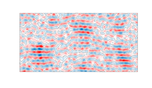
  $\alpha \sim 0.8$. The two-dimensional (2-D) wavenumber spectrum contains a well-pronounced peak at small zonal wavenumbers and an area of enhanced power at intermediate zonal wavenumbers (figure 1b). The leading EOF for this case displays prominent ZELTs (figure 1e); the autocorrelation (AC) function of the leading principal component (AC1) exhibits regular oscillations with the slight decay (figure 1h), thereby suggesting that ZELTs are persistent, low-frequency flow patterns. The other two flow regimes discussed below are characterized by the absence of ZELTs. In the isotropic regime with high bottom friction (
 $\gamma = 5\times 10^{-7}\ \mbox {s}^{-1},\beta = 1.14\times 10^{-11}\ \mbox {m}^{-1}\ \mbox {s}^{-1}$),
  $\alpha \ll 1$ and ZELTs are not observed (figure 1f). The 2-D wavenumber (Fourier) spectrum has a doughnut-like shape with the power distributed almost uniformly within a range of the total wavenumbers (figure 1c). The leading EOFs show chaotically distributed anomalies around the domain, and AC1 decays rapidly with time, indicating the lack of persistent patterns (figure 1i). Finally, we also consider the case with low bottom friction, for which
  $\alpha$ for the leading EOFs exhibits unexpectedly low value (
 $\gamma = 1\times 10^{-7}\ \mbox {s}^{-1},\beta = 2.15\times 10^{-11}\ \mbox {m}^{-1}\ \mbox {s}^{-1}$). We term this case as ‘quirky’ as it basically represents the special case reported in Rudko et al. (Reference Rudko, Kamenkovich, Iskadarani and Mariano2018) (see figure 18 in that paper). The spatial structure of the leading EOF displays rather irregular arrays of eddies and ZELTs are not visible (figure 1d). The spatial 2-D Fourier spectrum displays two areas with enhanced power, one that is situated at small zonal wavenumbers and the second that covers intermediate zonal wavenumbers and a wide range of meridional wavenumbers (figure 1a). Unlike the simulation with prominent ZELTs, whose spectrum has a somewhat similar shape, these two areas are well separated and the spectral peak at small zonal wavenumbers is not as intense. The AC1 for this case displays several oscillations with vanishing magnitude at a 12 000 day time lag (figure 1g). We note in passing that the ‘quirky’ regime is also characterized by prominent stationary zonal jets. The ZELT-dominated regime, therefore, corresponds to the intermediate values of bottom drag and can be interpreted as the transition from strongly anisotropic to isotropic turbulence.

Figure 1. The spatial Fourier spectra, leading EOF and AC function of leading principal component for model solution with the parameter values (a,d,g)  $\gamma = 1\times 10^{-7}\ \mbox {s}^{-1},\beta =2.15\times 10^{-11}\ \mbox {m}^{-1}\ \mbox {s}^{-1}$, (b,e,h)
  $\gamma = 3\times 10^{-7}\ \mbox {s}^{-1},\beta = 2.15\times 10^{-11}\ \mbox {m}^{-1}\ \mbox {s}^{-1}$ and (c,f,i)
  $\gamma = 5\times 10^{-7}\ \mbox {s}^{-1},\beta = 1.14\times 10^{-11}\ \mbox {m}^{-1}\ \mbox {s}^{-1}$.
We are closing this section by discussing the limitations of the quasi-geostrophic model. Simulations in a more realistic model would certainly entail some differences. ZELTs may not show up as leading EOF modes since the mesoscale variability can be obscured by the seasonal cycle and variability in the atmospheric forcing. Some additional filtering may be required to separate ZELTs from the background field. Nevertheless, non-stationary striations were reported in several general circulation model based studies (Richards et al. Reference Richards, Maximenko, Bryan and Sasaki2006; Kamenkovich, Berloff & Pedlosky Reference Kamenkovich, Berloff and Pedlosky2009; Melnichenko et al. Reference Melnichenko, Maximenko, Schneider and Sasaki2010). Most recently, ZELTs were also found in altimetry data by Chen, Kamenkovich & Berloff (Reference Chen, Kamenkovich and Berloff2016). We expect, however, that it suffices to use our two-layer quasi-geostrophic model to represent the dominant processes associated with the nonlinear baroclinic dynamics of ZELTs.
3. Steady state dynamics
We examine which nonlinear terms in the potential vorticity balance play dominant roles in the ZELT dynamics. This approach represents an extension of a similar analysis for stationary zonal jets (Kamenkovich et al. Reference Kamenkovich, Berloff and Pedlosky2009; Berloff et al. Reference Berloff, Kamenkovich and Pedlosky2009a). We apply our analysis to the barotropic and baroclinic balances for the zonally and time-dependent potential vorticity components (see appendix A). In order to quantify the impact of nonlinearity on ZELTs, we project the dynamical balance onto several leading EOFs of the streamfunction. Note that the same EOFs are used to define ZELTs in the study. Our main focus is on the advection of the potential vorticity, which represents the internally generated nonlinear forcing. This nonlinear forcing is due to interactions between eddies and mean state (EME) and due to interactions between eddies only ( $\mbox {EEE}$). The projections of the
  $\mbox {EME}$ components are
  $\mbox {F_MBT1}$,
  $\mbox {F_MBT2}$,
  $\mbox {F_MBC1}$,
  $\mbox {F_MBC2}$,
  $\mbox {F_MREL1}$,
  $\mbox {F_MREL2}$,
  $\mbox {F_MB1}$,
  $\mbox {F_MB2}$,
  $\mbox {F_MBC11}$,
  $\mbox {F_MBC12}$, the projections of
  $\mbox {EEE}$ components are
  $\mbox {F_EBT}$,
  $\mbox {F_EBC}$,
  $\mbox {F_EREL}$,
  $\mbox {F_EB}$,
  $\mbox {F_EBC1}$ (table 1). The acronyms follow these conventions:
  $\mbox {F}$ stands for forcing,
  $\mbox {M}$ – eddy–mean component,
  $\mbox {E}$ – eddy–eddy component,
  $\mbox {BT}$ – barotropic,
  $\mbox {BC}$ – baroclinic and
  $\mbox {MX}$ – mixed barotropic/baroclinic. When potential vorticity is further split into the relative vorticity and buoyancy terms we use
  $\mbox {REL}$ for the relative vorticity,
  $\mbox {B}$ for the buoyancy. All projections are conveniently summarized in table 1. We report on the magnitude of the projections (averaged in time) and on a time correlation between the projections of the tendency terms and the eddy forcing. The magnitude of the projections informs us of the relative contribution of each components of the nonlinear forcing to sustain ZELTs, while the correlations tell us whether the forcing works in favour or against ZELTs.
Table 1. Projection of the nonlinear forcing onto EOFs.  $\mbox {PV}$ – potential vorticity,
  $\mbox {RV}$ – relative vorticity.

In order to emphasize the particularity of the regime in which ZELTs appear as dominant modes of mesoscale variability, we carry out the analysis for three different cases discussed in the previous section. In line with Rudko et al. (Reference Rudko, Kamenkovich, Iskadarani and Mariano2018), who defined ZELTs as  $9$ leading EOFs, we consider the projections of
  $9$ EOFs in all three cases considered here as well. The
  $\mbox {EME}$ forcing dominates the eddy forcing in the low-friction case with no ZELTs (‘quirky’ case; figure 2(a,c)), thereby suggesting that the mean state imposes a strong control on the structure and magnitude of the eddying field. This is reminiscent of the ‘linear control’ reported in Berloff & Kamenkovich (Reference Berloff and Kamenkovich2013a,Reference Berloff and Kamenkovichb) in a similar regime. In contrast, the
  $\mbox {EEE}$ forcing dominates the eddy forcing in the ZELT-dominated regime, suggesting a strongly nonlinear dynamics (figure 3a,c). Both the
  $\mbox {EEE}$ and
  $\mbox {EME}$ forcing components are of the same order of magnitude in the isotropic turbulence simulation (figure 4a,c) with high bottom friction. In all cases, the projections of various components of the
  $\mbox {EME}$ forcing tend to cancel each other in both the barotropic and baroclinic modes (figures 2b, 3b, 4b).

Figure 2. The projection of different components of the nonlinear forcing onto the nine leading EOFs in the ‘quirky’ case: (a,b) barotropic mode, (c,d) baroclinic mode.

Figure 3. The projection of the different components of the nonlinear forcing onto the nine leading EOFs in the ZELT-dominated case: (a,b) barotropic mode, (c,d) baroclinic mode.

Figure 4. The projection of the different components of the nonlinear forcing onto the nine leading EOFs in the isotropic case: (a,b) barotropic mode, (c,d) baroclinic mode.
We next turn our attention to the specific  $\mbox {EEE}$ forcing components, contrasting the ZELT-dominated and isotropic regimes, since the eddy–eddy forcing is important in both cases. The
  $\mbox {EEE}$ forcing components in the barotropic balance always act in accord with each other in the ZELT-dominated case:
  $\mbox {F_EBT}$ and
  $\mbox {F_EBC}$ support all EOFs (figure 3a). The same is true in the isotropic regime (figure 4a). The
  $\mbox {EEE}$ forcing in the baroclinic balance exhibits a different behaviour. In the ZELT-dominated regime, advection of potential vorticity by baroclinic eddies,
  $\mbox {F_MX2}$ and
  $\mbox {F_EBC1}$ both resist ZELTs (figure 3b). In contrast, advection of eddy buoyancy
  $\mbox {F_EB}$ and eddy baroclinic relative vorticity
  $\mbox {F_EREL}$ by barotropic eddies always counteract each other, with
  $\mbox {F_EREL}$ supporting ZELTs and
  $\mbox {F_EB}$ resisting them. However, the magnitudes of the
  $\mbox {F_MX2}$ and
  $\mbox {F_EB}$ projections are higher than the projections of other
  $\mbox {EEE}$ forcings, thereby suggesting that, in a steady state, the dynamics of ZELTs is predominantly regulated by the advections of eddy barotropic potential vorticity and buoyancy,
  $\mbox {F_MX2}$ and
  $\mbox {F_EB}$ (figure 3b). The same two terms,
  $\mbox {F_MX2}$ and
  $\mbox {F_EB}$, also tend to be important in the isotropic regime, although the significance of
  $\mbox {F_EREL}$ and
  $\mbox {F_EBC1}$ is harder to establish.
In summary, the ZELT dynamics is dominated by the eddy forcing associated with eddy–eddy interactions, whereas the eddy–mean flow interactions play one of the leading roles in the cases with no ZELTs. Two eddy forcing components that are particularly important in the ZELT dynamics are the advection of eddy barotropic potential vorticity and eddy buoyancy,  $\mbox {F_MX2}$ and
  $\mbox {F_EB}$. In the next section, we explicitly examine the relative importance of various types of
  $\mbox {EEE}$ forcing for ZELT existence.
4. Reduced-dynamics models
In this section, we discuss simulations with fully or partially precluded  $\mbox {EEE}$ forcing, as it is this type of forcing that is associated with the cascades of eddy energy. Once can identify a group of
  $\mbox {EEE}$ terms that correspond to each type of eddy energy cascade. Setting these
  $\mbox {EEE}$ terms to zero in our numerical simulations effectively precludes the corresponding energy cascade. We consider four reduced-dynamics sensitivity experiments with: (a) precluded cascade of total eddy energy, (b) precluded eddy kinetic energy cascade in the barotropic mode, (c) precluded eddy kinetic energy cascade in the baroclinic mode, (d) precluded cascade of eddy potential energy. Table 2 lists the
  $\mbox {EEE}$ terms that are set to zero and corresponding energy cascades that are precluded in each of these sensitivity experiments. In all cases the net energy is preserved. The duration of each simulation and the values of parameters are the same as for the fully nonlinear simulations.
Table 2. Reduced-dynamics models.

The ZELT-dominated simulation with no eddy energy cascade exhibits a complete lack of power at the small zonal wavenumbers, implying the absence of ZELTs (figure 9a). The complete disappearance of ZELTs is further confirmed by the spatial structure of the the leading EOF, which displays meridionally elongated flow patterns similar to the most unstable mode of the baroclinically unstable background flow (figure 6a). The AC1 for this case (figure 12a) exhibits high-frequency variability, which is at odds with the evolution of AC1 in the fully nonlinear simulations. Similarly, the spectral power is dramatically reduced at small zonal wavenumbers in the cases with no ZELTs: the high-friction isotropic and ‘quirky’ cases (figures 8(a) and 10(a), respectively). These results suggest that the accumulation of energy at long zonal length scales in those two cases and the emergence of ZELTs in the ZELT-dominated case, are due to nonlinear interactions between eddies. This was expected for the ZELT-dominated regime simulations, because the  $\mbox {EEE}$ terms play a key role in the potential vorticity balance. The importance of
  $\mbox {EEE}$ interactions in the ‘quirky’ case may look surprising, given the fact that the potential vorticity balance is dominated by the eddy–mean flow interactions. Additionally, in both isotropic and ‘quirky’ cases, the leading EOF shows no signs of zonal anisotropy (figures 5a and 7a), while the AC1 indicates much higher temporal variability than in the fully nonlinear simulations (figures 11a and 13a).

Figure 5. Reduced-dynamics simulations for the ‘quirky’ case. Leading EOF for simulations with (a) no eddy energy transport, (b) no eddy kinetic energy transport in the barotropic mode, (c) no eddy kinetic energy transport in the baroclinic mode and (d) no eddy potential energy transport.
Removing the eddy kinetic energy cascade in the barotropic mode retains some spectral power at small zonal wavenumbers for the ZELT-dominated and ‘quirky’ cases (figures 8b and 9b). However, the leading EOF does not display zonally elongated patterns in either case, although the tendency of organization of the flow into chains of eddies (‘eddy trains’, Chen et al. (Reference Chen, Kamenkovich and Berloff2016)) is still discernible (figures 5b and 6b). AC1 shows rapid decay with ensuing fluctuating around zero, illustrating fast decorrelation of these eddies. In the isotropic case, the spatial Fourier spectrum bears a lot of resemblance to the spectrum of the fully nonlinear simulations (figure 5b). Interestingly, the leading EOF is anisotropic in this case (figure 7b). We recall that the barotropic eddy–eddy interactions are acting to enhance leading EOFs in the full isotropic simulation (figure 8), but these EOFs are isotropic. When the barotropic energy cascade is removed, these isotropic modes disappear and the latent anisotropy becomes visible.

Figure 6. Reduced-dynamics simulations for the ZELT-dominated case. Leading EOF for simulations with (a) no eddy energy transport, (b) no eddy kinetic energy transport in the barotropic mode, (c) no eddy kinetic energy transport in the baroclinic mode and (d) no eddy potential energy transport.

Figure 7. Reduced-dynamics simulations for the isotropic case. Leading EOF for simulations with (a) no eddy energy transport, (b) no eddy kinetic energy transport in the barotropic mode, (c) no eddy kinetic energy transport in the baroclinic mode and (d) no eddy potential energy transport.

Figure 8. Reduced-dynamics simulations for the ‘quirky’ case. Spatial Fourier spectra for simulations with (a) no eddy energy transport, (b) no eddy kinetic energy transport in the barotropic mode, (c) no eddy kinetic energy transport in the baroclinic mode and (d) no eddy potential energy transport.
The spectra for the simulation with no eddy kinetic energy cascade in the baroclinic mode resemble the simulation with no eddy energy transport: there is a negligible amount of spectral power at small zonal wavenumbers (figures 8c, 9c and 10c). It is interesting that the removal of the baroclinic energy cascade in the ZELT-dominated case leads to a significantly larger reduction in the spectral power than in the same case with no barotropic kinetic energy cascade. The leading EOF in all three cases display arrays of isolated eddies (figures 5c, 6c and 7c). The AC1 shows a slow decay in the ‘quirky’ and ZELT-dominated cases (figures 11c and 12c); the AC1 in the isotropic and fully nonlinear cases varies in a similar manner. We can certainly claim that the cascade of the eddy kinetic energy in the baroclinic mode plays a leading role in assisting the emergence of ZELTs in the ZELT-dominated case – the expected effect from the analysis of the potential vorticity balances in the previous section.

Figure 9. Reduced-dynamics simulations for the ZELT-dominated case. Spatial Fourier spectra for simulations with (a) no eddy energy transport, (b) no eddy kinetic energy transport in the barotropic mode, (c) no eddy kinetic energy transport in the baroclinic mode and (d) no eddy potential energy transport.

Figure 10. Reduced-dynamics simulations for the isotropic case. Spatial Fourier spectra for simulations with (a) no eddy energy transport, (b) no eddy kinetic energy transport in the barotropic mode, (c) no eddy kinetic energy transport in the baroclinic mode and (d) no eddy potential energy transport.

Figure 11. Reduced-dynamics simulations for the ‘quirky’ case. AC function for the leading principal component for simulations with (a) no eddy energy transport, (b) no eddy kinetic energy transport in the barotropic mode, (c) no eddy kinetic energy transport in the baroclinic mode and (d) no eddy potential energy transport.

Figure 12. Reduced-dynamics simulations for the ZELT-dominated case. AC function for the leading principal component for simulations with (a) no eddy energy transport, (b) no eddy kinetic energy transport in the barotropic mode, (c) no eddy kinetic energy transport in the baroclinic mode and (d) no eddy potential energy transport.
In both the ‘quirky’ and ZELT-dominated cases, the simulation with no eddy potential energy cascade exhibits spectral peaks at small zonal wavenumbers (figures 8d and 10d). The leading EOFs are zonally elongated in all three cases, including the isotropic regime (figures 5d, 6d and 7d). The AC1 exhibits a regular behaviour with rapidly decaying oscillations, two long oscillations and slowly decaying oscillations (figures 11d, 12d and 13d). We recall that the  $\mbox {F_EB}$ term plays a key role in the baroclinic potential vorticity balance, but acts to dissipate the flow patterns associated with the leading EOFs. It is, therefore, not surprising that the removal of the potential energy cascade enhances ZELTs in the ZELT-dominated case. The emergence of ZELTs in the isotropic and ‘quirky’ cases is an interesting result, suggesting that the potential energy cascade dissipates ZELTs and explains why they are not visible in either of the fully nonlinear simulations. Lastly, we note an overall similarity of the reduced-dynamics simulations in the ZELT-dominated and ‘quirky’ regimes.

Figure 13. Reduced-dynamics simulations for the isotropic case. AC function for the leading principal component for simulations with (a) no eddy energy transport, (b) no eddy kinetic energy transport in the barotropic mode, (c) no eddy kinetic energy transport in the baroclinic mode and (d) no eddy potential energy transport.
5. Summary and discussion
This study is concerned with the origins and mechanisms of mesoscale variability in the mid-latitude oceans. This mesoscale variability is anisotropic, and a previous study by Maltrud & Vallis (Reference Maltrud and Vallis1991) reported that the dominant modes of this variability have the form of ZELTs. ZELTs vary in the zonal direction and time and are, thus, different from stationary zonal jets that have been the subject of extensive studies of anisotropic turbulence. In this paper, we have elucidated the mechanisms governing the evolution of ZELTs, in the context of quasi-geostrophic turbulence. We used a two-layer, quasi-geostrophic model with a resolution of  $14\ \mbox {km}$. The governing equations are the conservation of layerwise potential vorticity with added bottom drag and viscosity. We have studied the dynamics of ZELTs using diagnostic (steady state dynamical balance) and prognostic approaches (reduced-dynamics simulations). We have studied three different flow regimes in which: (i) ZELTs appear as leading EOFs and the spectrum is anisotropic (ZELT-dominated case); (ii) the spatial structure of the leading EOFs and the spectrum is isotropic (isotropic case); and (iii) the leading EOFs display a quite irregular array of flow anomalies, but the spectrum is anisotropic (‘quirky’ case). The key findings of this study are that: (i) ZELTs are nonlinear phenomena that emerge as a result of eddy–eddy interactions; (ii) kinetic energy cascade is essential for ZELT emergence, with the baroclinic cascade being dominant; (iii) the potential energy cascade acts to damp ZELTs.
To distinguish ZELTs from previously studied zonal jets we decomposed the flow into zonally averaged (‘mean’) and deviation (‘eddy’) components. We have projected the governing equations onto several leading EOFs and analysed the projections of the nonlinear terms that are due to interactions between eddies (‘eddy–mean’ forcing) and the mean flow and between eddies only (‘eddy–eddy’ forcing). In the simulations with well-pronounced ZELTs (ZELT-dominated case), the eddy–eddy forcing dominates the potential vorticity balance: the largest contributing components are the divergences of the eddy barotropic vorticity flux and the eddy buoyancy flux. These components of eddy forcing entail the fluxes of eddy kinetic and eddy potential energies, and they tend to balance each other in all three regimes. In the ‘quirky’ case, the eddy–mean flow forcing dominates the dynamics, while the eddy–eddy interactions play a secondary role. This result is consistent with previous studies that reported the importance of the linear control in this flow regime (Berloff & Kamenkovich Reference Berloff and Kamenkovich2013a,Reference Berloff and Kamenkovichb) and the results of quasilinear theory (Farrell & Ioannou Reference Farrell and Ioannou2007, Reference Farrell and Ioannou2008; Srinivasan & Young Reference Srinivasan and Young2012). In the isotropic simulation, both types of nonlinear interaction are of the same order of magnitude.
To examine the importance of each type of energy transfer in the ZELT dynamics, we have considered several reduced-dynamics models, in which certain types of eddy–eddy interactions are truncated. Although the net energy is still conserved in all the experiments, the regimes they correspond to are different from the original simulations and are sensitive to the particular choice of truncation. The purpose of this exercise is to explore this sensitivity and demonstrate the importance of a specific type of energy exchange for the existence of ZELTs. The simulation with the removed transfer of the eddy energy shows no spectral power at small zonal wavenumbers and EOFs that are not zonally elongated. These results collectively demonstrate that ZELTs are a product of nonlinear interactions between eddies, confirming our conclusions from the analysis of the steady state nonlinear forcing. Analysis of the simulations, in which either the barotropic or baroclinic kinetic energy fluxes are blocked, also demonstrates the absence of ZELTs, confirming the importance of these types of energy cascades for ZELT emergence. The removal of the baroclinic cascade, however, leads to a particularly dramatic reduction in spectral power. Instead, the flow is dominated by eddies propagating along zonal tracks. These eddy trains have been reported previously in both model simulations and satellite data (Chen et al. Reference Chen, Kamenkovich and Berloff2016), and our results here further demonstrate that they become preferred modes of mesoscale variability once the kinetic energy cascade is suppressed.
Finally, the simulations with the removed cascade of the eddy potential energy show that the zonally elongated patterns are amplified and appear as dominating modes for all parameter choices of this study. Since the cascade of the eddy potential energy is directed downscale, and the corresponding term is shown to damp ZELTs, its removal leads to the accumulation of energy in the long scales. Additionally, the removal stops downward transfer the energy and weakens the energy dissipation by the bottom drag (Khatri & Berloff Reference Khatri and Berloff2018b). The change is particularly dramatic in isotropic and ‘quirky’ cases, which implies that this damping effect explains the lack of ZELTs in these regimes. The damping effect of the eddy buoyancy advection, compensated by the relative vorticity advection, is analogous to a similar balance in the stationary zonal jets, and is likely to be a fundamental property of anisotropic turbulence in the ocean. These results demonstrate the importance of baroclinic dynamics and the potential energy transfer, which are often ignored in the analysis of ocean energetics. This importance does not mean that ZELTs cannot be observed in barotropic flows. In fact, we expect zonally elongated modes of mesoscale variability to be ubiquitous in geostrophic turbulence with and without vertical stratification. For example, similar structures, termed ‘zonons’, have been observed in barotropic flows with small-scale forcing (Danilov & Gurarie Reference Danilov and Gurarie2004; Sukoriansky, Dikovskaya & Galperin Reference Sukoriansky, Dikovskaya and Galperin2008; Galperin & Sukoriansky & Dikovskaya Reference Galperin, Sukoriansky and Dikovskaya2010). Similarly, stationary zonal jets are prominent features of barotropic turbulence (Rhines Reference Rhines1994; Galperin et al. Reference Galperin, Nakano, Huang and Sukoriansky2004), despite the importance of buoyancy transfers for their baroclinic counterparts (Panetta Reference Panetta1993; Berloff et al. Reference Berloff, Kamenkovich and Pedlosky2009b).
The presence of the anisotropic flow patterns in oceanic circulation gives rise to asymmetry in the distribution of momentum, energy and oceanic tracers. Although the present study improves our understanding of the origins of anisotropy in mesoscale turbulence, the scope of the work is limited due to the simplicity of the model. Studies with general circulation models would definitely expand the current view on the issue.
Acknowledgement
The authors would like to thank M. Iskandarani for helping with model configuration.
Funding
M.R. was supported by NSF grant OCE-1154923. I.K. was supported by NOAA grant NA16OAR4310165.
Declaration of interests
The authors report no conflict of interest.
Appendix A. Dynamical balance
We derive the dynamical balance in several steps. First, the vertical structure of the two-layer quasi-geostrophic system can be fully described by the barotropic and the first baroclinic modes (Pedlosky Reference Pedlosky2013). The projection of the governing equations onto these two modes gives
 \begin{align} &\frac{\partial q_{p}}{\partial t}+J(\psi_{p},q_{p})+\theta_{11}\theta_{12}J(\psi_{c},q_{c})+\beta\frac{\partial\psi_{p}}{\partial x}+US_1\theta_{11}\frac{\partial\psi_{c}}{\partial x}\nonumber\\ &\quad =-U\theta_{11}\frac{\partial q_{p}}{\partial x}-U\theta_{11}\theta_{12}\frac{\partial q_{c}}{\partial x}-\gamma \theta_{12}q_{p}+\gamma\theta_{11}\theta_{12}\xi_{c}+\nu\nabla^2q_{p}, \end{align}
 \begin{align} &\frac{\partial q_{c}}{\partial t}+J(\psi_{p},q_{c})+J(\psi_{c},q_{p})+(\theta_{11}^2-\theta_{12}^2)J(\psi_{c},q_{c})\nonumber\\ &\qquad +(\beta+U(S_1\theta_{12}-S_2\theta_{11}))\frac{\partial\psi_{c}}{\partial x}+U(S_1+S_2)\frac{\partial\psi_{c}}{\partial x}\nonumber\\ &\quad =-U\frac{\partial q_{c}}{\partial x}-U\theta_{12}\frac{\partial q_{c}}{\partial x}-\gamma q_{p}+\gamma\theta_{11}\xi_{c}+\nu\nabla^2\xi_{c}, \end{align}
where
 \begin{align} \left.\begin{gathered} \theta_{11}=\frac{H_1}{H_1+H_2}=\frac{\dfrac{H_1}{H_2}}{\dfrac{H_1}{H_2}+1}=\frac{\delta}{\delta+1},\\ \theta_{12}=\frac{H_2}{H_1+H_2}=\frac{1}{\dfrac{H_1}{H_2}+1}=\frac{1}{\delta+1},\\ q_{p}=\nabla^2\frac{H_1\psi_1+H_2\psi_2}{H_1+H_2}=\nabla^2\psi_{p},\\ q_{c}=\nabla^2(\psi_1\,{-}\,\psi_2)\,{-}\,(S_1+S_2)(\psi_1\,{-}\,\psi_2)=\nabla^2\psi_{c}\,{-}\,(S_1+S_2)\psi_{c}=\xi_{c}\,{-}\,(S_1+S_2)\psi_{c}. \end{gathered}\right\} \end{align}
Decomposing the flow field into ‘mean’ (zonally averaged) and ‘eddy’ (deviation from zonally averaged) components leads to a set of four equations
 \begin{equation} \frac{\partial \overline{q_{p}}}{\partial t}=- \overline{J(\psi_{p}',q_{p}')}-\theta_{11}\theta_{12} \overline{J(\psi_{c}',q_{c}')}-\gamma \theta_{12}\overline{\xi_{p}}+\gamma\theta_{11}\theta_{12}\overline{\xi_{c}}+\nu\nabla^2\overline{\xi_{p}}, \end{equation}
 \begin{align} \frac{\partial q_{p}'}{\partial t}&=-J(\overline{\psi_{p}},q_{p}')\,{-}\,J(\psi_{p}',\overline{q_{p}})-J(\psi_{p}',q_{p}')'-\theta_{11}\theta_{12}[J(\overline{\psi_{c}},q_{c}')+J(\psi_{c}',\overline{q_{c}})+J(\psi_{c}',q_{c}')']\nonumber\\ &\quad-\beta\frac{\partial\psi_{p}'}{\partial x}-US_1\theta_{11}\frac{\partial\psi_{c}'}{\partial x}-U\theta_{11}\frac{\partial q_{p}'}{\partial x}-U\theta_{11}\theta_{12}\frac{\partial q_{c}'}{\partial x}\nonumber\\ &\quad -\gamma \theta_{12}\xi_{p}'+\gamma\theta_{11}\theta_{12}\xi_{c}'+\nu\nabla^2\xi_{p}', \end{align}
 \begin{equation} \frac{\partial \overline{q_{c}}}{\partial t}=-\overline{J(\psi_{p}',q_{c}')}-\overline{J(\psi_{c}',q_{p}')}-(\theta_{11}^2-\theta_{12}^2)\overline{J(\psi_{c}',q_{c}')}-\gamma \overline{\xi_{p}}+\gamma\theta_{11}\overline{\xi_{c}}+\nu\nabla^2\overline{\xi_{c}}, \end{equation}
 \begin{align} \frac{\partial q_{c}'}{\partial t}&=-J(\overline{\psi_{p}},q_{c})-J(\psi_{p}',\overline{q_{c}})-J(\psi_{p}',q_{c}')'-J(\overline{\psi_{c}},q_{p}')-J(\psi_{c}',\overline{q_{p}})-J(\psi_{c}',q_{p}')'\nonumber\\ &\quad-(\theta_{11}^2-\theta_{12}^2)[J(\overline{\psi_{c}},q_{c}')+J(\psi_{c}',\overline{q_{c}})+J(\psi_{c}',q_{c}')']\nonumber\\ &\quad-(\beta+U(S_1\theta_{12}-S_2\theta_{11}))\frac{\partial\psi_{c}'}{\partial x}-U(S_1+S_2)\frac{\partial\psi_{p}'}{\partial x}-U\frac{\partial q_{p}'}{\partial x}-U\theta_{12}\frac{\partial q_{c}'}{\partial x}\nonumber\\ &\quad-\gamma \xi_{p}'+\gamma\theta_{11}\xi_{c}'+\nu\nabla^2\xi_{c}' . \end{align}
Equations (A4) and (A6) describe the dynamics of stationary ( $\omega =0,k=0$) and drifting zonal jets (
 $\omega \neq 0,k=0$), while equations (A5) and (A7) govern the evolution of ‘eddies’ (
 $\omega \neq 0,k \neq 0$). Since ZELTs are a part of the ‘eddy’ flow component, we discuss equations (A5) and (A7) only. The left-hand sides of these equations are the tendency terms, which describe the rate of change in the ‘eddy’ potential vorticity, whereas the right-hand side consists of several nonlinear terms (‘eddy forcing’), as well as linear terms that contain the modified
  $\beta$-terms, external forcing terms and large- and small-scale friction.


