


1 Introduction
The problem of a two-dimensional flow around an infinitely long thin plate performing harmonic oscillations in a viscous incompressible fluid is a classical hydrodynamic problem. Its solutions are widely used for estimation of the characteristics of fluid–structure interaction processes and for determination of the parameters of flows caused by oscillations of structures in studies of complex dynamical systems in a variety of subject areas, such as the construction of oil platforms (e.g. Tao & Thiagarajan Reference Tao and Thiagarajan2003a ,Reference Tao and Thiagarajan b ), development of biomimetic underwater propulsion systems (e.g. Kopman & Porfiri Reference Kopman and Porfiri2013), generation of electric energy (e.g. Aureli et al. Reference Aureli, Prince, Porfiri and Peterson2010; Erturk & Inman Reference Erturk and Inman2011), damping of oscillations in fuel tanks (e.g. Buzhinskii Reference Buzhinskii1998a ,Reference Buzhinskii b ), development of cooling systems of electronic boards (e.g. Bidkar et al. Reference Bidkar, Kimber, Raman, Bajaj and Garimella2009), study of properties of materials (e.g. Egorov et al. Reference Egorov, Kamalutdinov, Nuriev and Paimushin2014; Paimushin et al. Reference Paimushin, Firsov, Gyunal, Egorov and Kayumov2014; Paimushin, Firsov & Shishkin Reference Paimushin, Firsov and Shishkin2017), etc.
Analytical solutions of the problem which cover the entire range of geometric and frequency parameters are available today only for the range of small oscillation amplitudes, where the fluid dynamics around the plate can be described in a linear approximation (see Kanwal Reference Kanwal1955; Tuck Reference Tuck1969). In the range of large and moderate oscillation amplitudes, where the external flow is determined by the nonlinear interaction of complex vortex structures forming near the plate, the key methods of investigation are experiments and numerical simulation.
Experimental results are the main source of estimates of the hydrodynamic forces acting on the plate today. A significant part of the information about the problem was obtained in classical hydrodynamic experiments conducted in the 60–80s of the last century (see Keulegan & Carpenter Reference Keulegan and Carpenter1958; Bearman Reference Bearman1971; Bearman, Graham & Singh Reference Bearman, Graham and Singh1979; Singh Reference Singh1979; Bearman & Obasaju Reference Bearman and Obasaju1982; Bearman et al. Reference Bearman, Downie, Graham and Obasaju1985). The main goals of these pioneer researcher were: (i) identification of the main control parameters of the oscillatory process; (ii) evaluation of the hydrodynamic forces acting on the plates; (iii) observation of the flow structure near the oscillating plates.
In the course of numerous experiments with cylindrical bodies of different cross-sections, it was established that the key similarity parameters of flows near bodies with the same geometric characteristics are the following complexes
 $$\begin{eqnarray}\displaystyle KC=2\unicode[STIX]{x03C0}{\displaystyle \frac{U_{0}}{b\unicode[STIX]{x1D714}}}=2\unicode[STIX]{x03C0}{\displaystyle \frac{A}{b}},\quad \unicode[STIX]{x1D6FD}={\displaystyle \frac{b^{2}\unicode[STIX]{x1D714}}{2\unicode[STIX]{x03C0}\unicode[STIX]{x1D708}}}. & & \displaystyle\end{eqnarray}$$
Where
 $A$
and
$A$
and
 $U_{0}=A\unicode[STIX]{x1D714}$
represent the amplitude of the oscillations and the amplitude of the velocity of oscillations, respectively,
$U_{0}=A\unicode[STIX]{x1D714}$
represent the amplitude of the oscillations and the amplitude of the velocity of oscillations, respectively,
 $b$
is a characteristic length scale (a width of the plate for the considered case),
$b$
is a characteristic length scale (a width of the plate for the considered case),
 $\unicode[STIX]{x1D714}$
is the angular frequency and
$\unicode[STIX]{x1D714}$
is the angular frequency and
 $\unicode[STIX]{x1D708}$
is the kinematic viscosity of the fluid.
$\unicode[STIX]{x1D708}$
is the kinematic viscosity of the fluid.
The parameter
 $KC$
is called the Keulegan–Carpenter number, it characterizes the dimensionless amplitude of the oscillations. According to the results of Bearman et al. (Reference Bearman, Downie, Graham and Obasaju1985) this parameter almost completely determines the solution of the problem for large oscillation amplitudes. The second parameter
$KC$
is called the Keulegan–Carpenter number, it characterizes the dimensionless amplitude of the oscillations. According to the results of Bearman et al. (Reference Bearman, Downie, Graham and Obasaju1985) this parameter almost completely determines the solution of the problem for large oscillation amplitudes. The second parameter
 $\unicode[STIX]{x1D6FD}$
is often called the Stokes number or vibrational Reynolds number, it can be interpreted as the dimensionless oscillation frequency. A significant influence of this parameter on the oscillation process is manifested at small and moderate amplitudes. Notice that the structure of the flows and the magnitude of the forces at the same values of the parameters for profiles of different shapes are extremely different, for example, the drag of the square cylinder and the thin plate at large amplitudes of oscillations differ by more than a factor of two (see Singh Reference Singh1979; Bearman et al.
Reference Bearman, Downie, Graham and Obasaju1985).
$\unicode[STIX]{x1D6FD}$
is often called the Stokes number or vibrational Reynolds number, it can be interpreted as the dimensionless oscillation frequency. A significant influence of this parameter on the oscillation process is manifested at small and moderate amplitudes. Notice that the structure of the flows and the magnitude of the forces at the same values of the parameters for profiles of different shapes are extremely different, for example, the drag of the square cylinder and the thin plate at large amplitudes of oscillations differ by more than a factor of two (see Singh Reference Singh1979; Bearman et al.
Reference Bearman, Downie, Graham and Obasaju1985).
The parametrization of the measured forces in oscillatory motion is a non-trivial task. For this purpose in the works of Keulegan & Carpenter (Reference Keulegan and Carpenter1958), Bearman et al. (Reference Bearman, Graham and Singh1979), Singh (Reference Singh1979), Bearman et al. (Reference Bearman, Downie, Graham and Obasaju1985), Morison’s approach (Morison, Johnson & Schaaf Reference Morison, Johnson and Schaaf1950) was chosen. According to which the force
 $F_{x}$
acting on the oscillating body in the fluid along the axis of oscillation is represented as the sum of the drag force, proportional to the velocity, and the inertia force, proportional to the acceleration of the oscillatory motion
$F_{x}$
acting on the oscillating body in the fluid along the axis of oscillation is represented as the sum of the drag force, proportional to the velocity, and the inertia force, proportional to the acceleration of the oscillatory motion
 $$\begin{eqnarray}\displaystyle F_{x}={\textstyle \frac{1}{4}}\unicode[STIX]{x1D70C}\unicode[STIX]{x03C0}b^{2}C_{M}\dot{U}_{p}+{\textstyle \frac{1}{2}}\unicode[STIX]{x1D70C}bC_{D}U_{p}|U_{p}|. & & \displaystyle\end{eqnarray}$$
Where
 $\unicode[STIX]{x1D70C}$
is the density of the fluid,
$\unicode[STIX]{x1D70C}$
is the density of the fluid,
 $U_{p},\dot{U}_{p}$
are the velocity and the acceleration of the motion,
$U_{p},\dot{U}_{p}$
are the velocity and the acceleration of the motion,
 $C_{D},C_{M}$
are the coefficients of the drag and inertia forces, respectively.
$C_{D},C_{M}$
are the coefficients of the drag and inertia forces, respectively.
Despite similar concepts of research methods and data analysis, on comparing the results obtained in classical experiments by different groups of researchers (Keulegan & Carpenter Reference Keulegan and Carpenter1958; Bearman et al.
Reference Bearman, Graham and Singh1979; Singh Reference Singh1979; Bearman et al.
Reference Bearman, Downie, Graham and Obasaju1985), it is possible to detect significant differences (up to 30 %) in estimation of the drag coefficient of the plate in the zone of moderately large values of the dimensionless amplitude
 $KC$
. These differences are explained by Singh (Reference Singh1979) as a result of incomplete agreement of other parameters of the experiments, such as the frequency range and geometric characteristics of the plates. It is not possible to completely identify the effects of these parameters from experimental data of Keulegan & Carpenter (Reference Keulegan and Carpenter1958), Singh (Reference Singh1979), Bearman et al. (Reference Bearman, Downie, Graham and Obasaju1985). The geometric characteristics of the samples in the work (Keulegan & Carpenter Reference Keulegan and Carpenter1958) are unknown. In the works of Singh (Reference Singh1979), Bearman et al. (Reference Bearman, Downie, Graham and Obasaju1985), plates with chamfered edges and different relative thickness
$KC$
. These differences are explained by Singh (Reference Singh1979) as a result of incomplete agreement of other parameters of the experiments, such as the frequency range and geometric characteristics of the plates. It is not possible to completely identify the effects of these parameters from experimental data of Keulegan & Carpenter (Reference Keulegan and Carpenter1958), Singh (Reference Singh1979), Bearman et al. (Reference Bearman, Downie, Graham and Obasaju1985). The geometric characteristics of the samples in the work (Keulegan & Carpenter Reference Keulegan and Carpenter1958) are unknown. In the works of Singh (Reference Singh1979), Bearman et al. (Reference Bearman, Downie, Graham and Obasaju1985), plates with chamfered edges and different relative thickness
 $\unicode[STIX]{x1D6E5}\approx 0.31,0.21,0.1$
are used, where
$\unicode[STIX]{x1D6E5}\approx 0.31,0.21,0.1$
are used, where
 $\unicode[STIX]{x1D6E5}$
is defined as the ratio of the plate thickness
$\unicode[STIX]{x1D6E5}$
is defined as the ratio of the plate thickness
 $h$
to its width
$h$
to its width
 $b$
$b$
 $$\begin{eqnarray}\displaystyle \unicode[STIX]{x1D6E5}=h/b. & & \displaystyle\end{eqnarray}$$
However, each sample was tested only at one value of dimensionless frequency:
 $\unicode[STIX]{x1D6FD}=188$
(for
$\unicode[STIX]{x1D6FD}=188$
(for
 $\unicode[STIX]{x1D6E5}\approx 0.31$
),
$\unicode[STIX]{x1D6E5}\approx 0.31$
),
 $\unicode[STIX]{x1D6FD}=421.5$
(for
$\unicode[STIX]{x1D6FD}=421.5$
(for
 $\unicode[STIX]{x1D6E5}\approx 0.21$
),
$\unicode[STIX]{x1D6E5}\approx 0.21$
),
 $\unicode[STIX]{x1D6FD}=1685.8$
(for
$\unicode[STIX]{x1D6FD}=1685.8$
(for
 $\unicode[STIX]{x1D6E5}\approx 0.1$
).
$\unicode[STIX]{x1D6E5}\approx 0.1$
).
The descriptions of the flow structures in the vicinity of oscillating thin plates, obtained from the results of investigations (Keulegan & Carpenter Reference Keulegan and Carpenter1958; Singh Reference Singh1979) in general are identical. The most complete information is given in the research of Singh (Reference Singh1979). According to its results, it is possible to distinguish four main flow regimes which can be localized in the following ranges of values of the parameter
 $KC$
:
$KC$
:
 $0<KC<3$
is the range of symmetric flows,
$0<KC<3$
is the range of symmetric flows,
 $3<KC<7$
is the range of asymmetric flows,
$3<KC<7$
is the range of asymmetric flows,
 $7<KC<25$
is range of ‘cyclic’ flows,
$7<KC<25$
is range of ‘cyclic’ flows,
 $KC>25$
is range of ‘pseudo-Kármán vortex street’ development.
$KC>25$
is range of ‘pseudo-Kármán vortex street’ development.
Another type of experimental source is the modern works of Egorov et al. (Reference Egorov, Kamalutdinov, Nuriev and Paimushin2017), Egorov, Kamalutdinov & Nuriev (Reference Egorov, Kamalutdinov and Nuriev2018), Shrestha, Ahsan & Aureli (Reference Shrestha, Ahsan and Aureli2018) where the two-dimensional flows around long thin beams performing flexural vibrations in a fluid were investigated. The motion of a fluid near each beam cross-section at low oscillation modes in a limited range of oscillation amplitudes has a two-dimensional structure that is equivalent to a flow near a harmonically oscillating thin rigid plate. On the basis of this concept Egorov et al. (Reference Egorov, Kamalutdinov, Nuriev and Paimushin2017, Reference Egorov, Kamalutdinov and Nuriev2018) purposed a theoretical–experimental method for determination of the hydrodynamic drag and inertial forces acting on cantilever beams performing free vibrations in the air. The experiments were performed in the range
 $0<KC<6$
,
$0<KC<6$
,
 $50<\unicode[STIX]{x1D6FD}<1500$
. As test samples, beams with chamfered edges and a relative thickness of
$50<\unicode[STIX]{x1D6FD}<1500$
. As test samples, beams with chamfered edges and a relative thickness of
 $0.03<\unicode[STIX]{x1D6E5}<0.1$
were used. The obtained estimates of the drag forces have a good agreement with the data of Singh (Reference Singh1979). In addition, for
$0.03<\unicode[STIX]{x1D6E5}<0.1$
were used. The obtained estimates of the drag forces have a good agreement with the data of Singh (Reference Singh1979). In addition, for
 $C_{D}$
in the studied range of parameters, an approximation formula that describes the dependence of this coefficient from the parameters
$C_{D}$
in the studied range of parameters, an approximation formula that describes the dependence of this coefficient from the parameters
 $\unicode[STIX]{x1D6FD}$
and
$\unicode[STIX]{x1D6FD}$
and
 $KC$
was proposed.
$KC$
was proposed.
Shrestha et al. (Reference Shrestha, Ahsan and Aureli2018) on the basis of particle image velocimetry (PIV) technology studied the structure of the flow near the oscillating beam and calculated the hydrodynamic forces acting on the beam. The experiments were performed in the zone of small and moderate oscillation amplitudes
 $0.06<KC<5.7$
in the frequency range
$0.06<KC<5.7$
in the frequency range
 $20\leqslant \unicode[STIX]{x1D6FD}\leqslant 1800$
for rectangular samples with relative thickness of
$20\leqslant \unicode[STIX]{x1D6FD}\leqslant 1800$
for rectangular samples with relative thickness of
 $\unicode[STIX]{x1D6E5}=0.04$
. Based on the results, a flow regime map was constructed which includes five different regimes. The boundaries of the regimes are highly dependent on the frequency and the amplitude of the oscillations. It should be noted that the upper boundary of symmetry flows in the range of moderate frequencies
$\unicode[STIX]{x1D6E5}=0.04$
. Based on the results, a flow regime map was constructed which includes five different regimes. The boundaries of the regimes are highly dependent on the frequency and the amplitude of the oscillations. It should be noted that the upper boundary of symmetry flows in the range of moderate frequencies
 $\unicode[STIX]{x1D6FD}>300$
was localized in the region
$\unicode[STIX]{x1D6FD}>300$
was localized in the region
 $KC<0.8$
, which is at least 3.5 times less than the estimate of Singh (Reference Singh1979).
$KC<0.8$
, which is at least 3.5 times less than the estimate of Singh (Reference Singh1979).
Along with experimental studies, the numerical methods for the solution of the problem of flow past a harmonic oscillating thin plate has been developing for a fairly long time. Significant progress in these studies was achieved for the region of small oscillation amplitudes. In the works of Aureli & Porfiri (Reference Aureli and Porfiri2010), Aureli, Porfiri & Basaran (Reference Aureli, Porfiri and Basaran2012), Phan, Aureli & Porfiri (Reference Phan, Aureli and Porfiri2013) on the basis of traditional mesh methods the solution of the problem of the oscillations of rectangular plates in the range of the parameters
 $0.1\leqslant \unicode[STIX]{x1D6E5}\leqslant 10.003\leqslant <KC\leqslant 0.3$
was carried out. The obtained results describe the beginning of the development of nonlinear hydrodynamic processes near the plate and their influence on the hydrodynamic forces. All the numerical data in this area have a good agreement with each other and almost completely fill the gaps of experimental and analytical studies.
$0.1\leqslant \unicode[STIX]{x1D6E5}\leqslant 10.003\leqslant <KC\leqslant 0.3$
was carried out. The obtained results describe the beginning of the development of nonlinear hydrodynamic processes near the plate and their influence on the hydrodynamic forces. All the numerical data in this area have a good agreement with each other and almost completely fill the gaps of experimental and analytical studies.
Numerical studies of flows in the region of large amplitudes do not have such unambiguous results. The first attempts to simulate the separated flow for the large amplitude vibrations of plates were taken by Graham (Reference Graham1980). Using the discrete-point-vortex method the author described the development of the vortex structure in the vicinity of the edges of the plate, that was similar to the observed in the ‘cyclic’ flow regime of Singh (Reference Singh1979). However, the estimates of the drag forces acting on the plate have the only qualitative agreement with the experimental data of Singh (Reference Singh1979). The inviscid vortex-shedding model was used to describe the fluid motion around the oscillating plate by Bidkar et al. (Reference Bidkar, Kimber, Raman, Bajaj and Garimella2009). The solutions found in this study had a symmetric structure with respect to the oscillation axis in the range
 $0<KC<5$
. The calculated values of the hydrodynamic forces acting on the plate were also significantly higher than estimates obtained in the experimental works.
$0<KC<5$
. The calculated values of the hydrodynamic forces acting on the plate were also significantly higher than estimates obtained in the experimental works.
Numerical models of Tafuni & Sahin (Reference Tafuni and Sahin2015) (based on smoothed particle hydrodynamics), De Rosis & Lévêque (Reference De Rosis and Lévêque2015) (based on Lattice Boltzmann method), Egorov et al. (Reference Egorov, Kamalutdinov, Nuriev and Paimushin2014) (based on finite volume method) give a qualitatively better agreement with experiments in the field of hydrodynamic force estimations. The results of calculation of the drag force acting on oscillating rectangular plates, performed in the paper Egorov et al. (Reference Egorov, Kamalutdinov, Nuriev and Paimushin2014) in the range of parameters
 $0<KC<6$
,
$0<KC<6$
,
 $50<\unicode[STIX]{x1D6FD}<1500$
, are in good agreement with the experimental results of Keulegan & Carpenter (Reference Keulegan and Carpenter1958). At the same time, the data obtained in the work do not explain more than 30 % of the difference from the results of Singh (Reference Singh1979), Egorov et al. (Reference Egorov, Kamalutdinov and Nuriev2018) and do not describe the development of the flow structure. Representations of flow regimes near the plate obtained by Tafuni & Sahin (Reference Tafuni and Sahin2015) (
$50<\unicode[STIX]{x1D6FD}<1500$
, are in good agreement with the experimental results of Keulegan & Carpenter (Reference Keulegan and Carpenter1958). At the same time, the data obtained in the work do not explain more than 30 % of the difference from the results of Singh (Reference Singh1979), Egorov et al. (Reference Egorov, Kamalutdinov and Nuriev2018) and do not describe the development of the flow structure. Representations of flow regimes near the plate obtained by Tafuni & Sahin (Reference Tafuni and Sahin2015) (
 $200<\unicode[STIX]{x1D6FD}<2000$
,
$200<\unicode[STIX]{x1D6FD}<2000$
,
 $0.1<KC<4.4$
) and De Rosis & Lévêque (Reference De Rosis and Lévêque2015) (
$0.1<KC<4.4$
) and De Rosis & Lévêque (Reference De Rosis and Lévêque2015) (
 $200<\unicode[STIX]{x1D6FD}<2000$
,
$200<\unicode[STIX]{x1D6FD}<2000$
,
 $0<KC<4.4$
) significantly differ from the experimental data of Singh (Reference Singh1979), Shrestha et al. (Reference Shrestha, Ahsan and Aureli2018). In Tafuni & Sahin (Reference Tafuni and Sahin2015), as in De Rosis & Lévêque (Reference De Rosis and Lévêque2015) the symmetric flow regimes remain stable throughout the investigated range of oscillation amplitudes. This is an order of magnitude greater than the estimates of the boundary of the symmetry regimes obtained by Shrestha et al. (Reference Shrestha, Ahsan and Aureli2018).
$0<KC<4.4$
) significantly differ from the experimental data of Singh (Reference Singh1979), Shrestha et al. (Reference Shrestha, Ahsan and Aureli2018). In Tafuni & Sahin (Reference Tafuni and Sahin2015), as in De Rosis & Lévêque (Reference De Rosis and Lévêque2015) the symmetric flow regimes remain stable throughout the investigated range of oscillation amplitudes. This is an order of magnitude greater than the estimates of the boundary of the symmetry regimes obtained by Shrestha et al. (Reference Shrestha, Ahsan and Aureli2018).
From the above analysis of the literature we can reveal the following problematic aspects in the study of fluid flows induced by the oscillations of thin plates and evaluation of their influence on the oscillator: (i) the determination of the influence of the parameters of the problem (including the geometric characteristics of the plate) on the hydrodynamic forces; (ii) the determination of the structure of the flow around the plates and their boundaries in the parametric domain of the problem; (iii) the determination of the reasons for the mismatch of estimates of hydrodynamic drag in the experiments of Singh (Reference Singh1979), Egorov et al. (Reference Egorov, Kamalutdinov and Nuriev2018) and Keulegan & Carpenter (Reference Keulegan and Carpenter1958), Egorov et al. (Reference Egorov, Kamalutdinov, Nuriev and Paimushin2014). These aspects form the subject of the present study.
In present work the hydrodynamic processes occurring during the oscillatory motion of plates are studied numerically. The fluid motion around the plates is described by a non-stationary system of Navier–Stokes equations. The numerical scheme of the solution is constructed on the basis of the finite volume method.
The paper is organized as follows. The mathematical formulation of the problem is given in § 2. In § 3 a numerical scheme and its verification are presented. The structure of flows around the plates at different oscillation parameters are discussed in § 5, in § 6 the analysis of the influence of the oscillation parameters and the geometry of the plates on the hydrodynamic forces is carried out. Concluding remarks are given in § 7. In the Appendix the importance of three-dimensional effects which may appear in the investigated range of parameters is also discussed.
2 Mathematical formulation of the problem
Consider a thin long plate that oscillates in a viscous incompressible fluid. The velocity of oscillation varies according to the harmonic law
 $$\begin{eqnarray}\displaystyle U_{p}=U_{0}\cos (\unicode[STIX]{x1D714}\tilde{t}). & & \displaystyle\end{eqnarray}$$
The aims of the research are the study of two-dimensional flows which form around the plate and the analysis of hydrodynamic forces caused by these flows for a wide range of oscillation parameters and geometrical characteristics of the plate.
We consider three different types of plates: plates with a rectangular cross-section (type I), plates with chamfered edges (type II) and plates with rounded edges (type III). Schematic representation of the plates of each type is shown in figure 1. As geometric similarity parameters, the relative thickness
 $\unicode[STIX]{x1D6E5}$
(for samples of all three types), the vertex angle
$\unicode[STIX]{x1D6E5}$
(for samples of all three types), the vertex angle
 $\unicode[STIX]{x1D6FC}=60^{\circ }$
for the plates with chamfered edges and the dimensionless corner radius
$\unicode[STIX]{x1D6FC}=60^{\circ }$
for the plates with chamfered edges and the dimensionless corner radius
 $R=r/h$
for rounded samples are used.
$R=r/h$
for rounded samples are used.

Figure 1. Geometrical characteristics of plates.
We solve the problem in a moving Cartesian coordinate system rigidly connected with the plate. The axis
 $Ox$
of moving coordinate system coincides with the axis of oscillation of the plate. Normalizing the spatial coordinates, time and velocity by
$Ox$
of moving coordinate system coincides with the axis of oscillation of the plate. Normalizing the spatial coordinates, time and velocity by
 $b$
,
$b$
,
 $b{U_{0}}^{-1}$
,
$b{U_{0}}^{-1}$
,
 $-U_{0}$
, respectively, we write the system of equations of motion for the fluid in the following form:
$-U_{0}$
, respectively, we write the system of equations of motion for the fluid in the following form:
 $$\begin{eqnarray}\displaystyle \left.\begin{array}{@{}c@{}}\displaystyle {\displaystyle \frac{\unicode[STIX]{x2202}\boldsymbol{U}}{\unicode[STIX]{x2202}t}}+\boldsymbol{U}\boldsymbol{\cdot }\unicode[STIX]{x1D735}\boldsymbol{U}=-\unicode[STIX]{x1D735}p+{\displaystyle \frac{1}{KC\unicode[STIX]{x1D6FD}}}\unicode[STIX]{x1D6FB}^{2}\boldsymbol{U},\\ \displaystyle \unicode[STIX]{x1D735}\boldsymbol{\cdot }\boldsymbol{U}=0.\end{array}\right\} & & \displaystyle\end{eqnarray}$$
Here
 $\boldsymbol{U}=(u,v)$
is dimensionless velocity,
$\boldsymbol{U}=(u,v)$
is dimensionless velocity,
 $p$
is fictitious pressure, that equals to the sum of the true pressure
$p$
is fictitious pressure, that equals to the sum of the true pressure
 $\tilde{p}$
and the inertial component
$\tilde{p}$
and the inertial component
 $\bar{p}$
, which occurs as a result of the transition to the moving coordinate system (see, e.g. Dutsch et al.
Reference Dutsch, Durst, Becker and Lienhart1998) and can be defined as
$\bar{p}$
, which occurs as a result of the transition to the moving coordinate system (see, e.g. Dutsch et al.
Reference Dutsch, Durst, Becker and Lienhart1998) and can be defined as
 $$\begin{eqnarray}\displaystyle \bar{p}=x{\displaystyle \frac{2\unicode[STIX]{x03C0}}{KC}}\sin \left({\displaystyle \frac{2\unicode[STIX]{x03C0}}{KC}}t\right). & & \displaystyle\end{eqnarray}$$
Dimensionless parameters
 $\unicode[STIX]{x1D6FD}$
and
$\unicode[STIX]{x1D6FD}$
and
 $KC$
are defined according to the formulas (1.1).
$KC$
are defined according to the formulas (1.1).
On the boundary of the plate in the new coordinate system no-slip conditions are specified,
 $$\begin{eqnarray}\displaystyle u_{S}=v_{S}=0. & & \displaystyle\end{eqnarray}$$
At infinity the change of the velocity is given by the harmonic law
 $$\begin{eqnarray}\displaystyle u_{\infty }=\cos \left({\displaystyle \frac{2\unicode[STIX]{x03C0}}{KC}}t\right),\quad v_{\infty }=0. & & \displaystyle\end{eqnarray}$$
The calculation of hydrodynamic forces and the moment acting on the plate in the presented dimensionless formulation is carried out according to the formulas
 $$\begin{eqnarray}\displaystyle \left.\begin{array}{@{}c@{}}\displaystyle \boldsymbol{F}=\int _{S}p\boldsymbol{n}\,\text{d}s-\int _{S}\unicode[STIX]{x1D640}\boldsymbol{\cdot }\boldsymbol{n}\,\text{d}s,\\ \displaystyle \boldsymbol{M}=\int _{S}\boldsymbol{r}_{\mathbf{0}}\times p\boldsymbol{n}\,\text{d}s-\int _{S}\boldsymbol{r}_{\mathbf{0}}\times \unicode[STIX]{x1D640}\boldsymbol{\cdot }\boldsymbol{n}\,\text{d}s,\end{array}\right\} & & \displaystyle\end{eqnarray}$$
where
 $\unicode[STIX]{x1D640}$
is a viscous stress tensor,
$\unicode[STIX]{x1D640}$
is a viscous stress tensor,
 $S$
is the surface of the plate,
$S$
is the surface of the plate,
 $\boldsymbol{n}$
is the inward-pointing unit normal vector to the plate surface and
$\boldsymbol{n}$
is the inward-pointing unit normal vector to the plate surface and
 $\boldsymbol{r}_{\mathbf{0}}$
is a radius vector directed from the geometric centre the plate to its surface. It should be noted that the force in the moving coordinate system is determined by the fictitious pressure and therefore contains a contribution from the inertial component
$\boldsymbol{r}_{\mathbf{0}}$
is a radius vector directed from the geometric centre the plate to its surface. It should be noted that the force in the moving coordinate system is determined by the fictitious pressure and therefore contains a contribution from the inertial component
 $\bar{p}$
(2.3). This contribution can be calculated as follows:
$\bar{p}$
(2.3). This contribution can be calculated as follows:
 $$\begin{eqnarray}\displaystyle \boldsymbol{F}_{fk}={\displaystyle \frac{2\unicode[STIX]{x03C0}}{KC}}\sin \left({\displaystyle \frac{2\unicode[STIX]{x03C0}}{KC}}t\right)\int _{S}x\boldsymbol{n}\,\text{d}s. & & \displaystyle\end{eqnarray}$$
It is also known as the Froude–Krylov force.
To analyse the in-line force, we use Morrison’s approximation (1.2). In dimensionless variables, it can be rewritten as follows:
 $$\begin{eqnarray}\displaystyle F_{x}={\displaystyle \frac{\unicode[STIX]{x03C0}}{2}}C_{M}{\displaystyle \frac{\text{d}u_{\infty }}{\text{d}t}}+C_{D}|u_{\infty }|u_{\infty }. & & \displaystyle\end{eqnarray}$$
The calculation of the hydrodynamic coefficients
 $C_{D},C_{M}$
is carried out at each oscillation period
$C_{D},C_{M}$
is carried out at each oscillation period
 $T$
by integration
$T$
by integration
 $$\begin{eqnarray}\displaystyle C_{M}=-{\displaystyle \frac{1}{\unicode[STIX]{x03C0}^{2}}}\int _{t_{0}}^{T+t_{0}}F_{x}\sin \left({\displaystyle \frac{2\unicode[STIX]{x03C0}}{KC}}t\right)\text{d}t,\quad C_{D}={\displaystyle \frac{3\unicode[STIX]{x03C0}}{8KC}}\int _{t_{0}}^{T+t_{0}}F_{x}\cos \left({\displaystyle \frac{2\unicode[STIX]{x03C0}}{KC}}t\right)\text{d}t.\quad & & \displaystyle\end{eqnarray}$$
3 Numerical scheme
The solution of the resulting governing system of (2.2), (2.4), (2.5) was carried out numerically. For discretization of the equations we used the finite volume method. The realization of the computation scheme was done on the basis of the OpenFOAM package (Greenshields Reference Greenshields2018).
The plane of flow
 $xOy$
was limited to a rectangular region of size
$xOy$
was limited to a rectangular region of size
 $(l_{x},l_{y})$
which sides were set parallel to the main axes of coordinates. The plate was placed in the centre of the computational domain and coordinate system. The discretization of the computational domain was carried out using block meshes. The cells of mesh in the flow plane had a quadrilateral shape. The resolution near the plate was controlled by the linear mesh grading in the directions normal to the sides of the plate and by successive refinement of the cells in the vicinity of its boundaries by cutting them into four parts (see figure 2).
$(l_{x},l_{y})$
which sides were set parallel to the main axes of coordinates. The plate was placed in the centre of the computational domain and coordinate system. The discretization of the computational domain was carried out using block meshes. The cells of mesh in the flow plane had a quadrilateral shape. The resolution near the plate was controlled by the linear mesh grading in the directions normal to the sides of the plate and by successive refinement of the cells in the vicinity of its boundaries by cutting them into four parts (see figure 2).

Figure 2. The structure of the mesh in the vicinity of the plate edge.
Simulation of the flow around rectangular plates and plates with chamfered and rounded edges were carried out on identical meshes. The differences between meshes were only in the small zones near the edges of plates. The values of the main parameters of the applied meshes are given in the table 1, where
 $N$
is the total number of cells,
$N$
is the total number of cells,
 $V_{min}$
is the minimum volume of cells in the boundary layer of the plate,
$V_{min}$
is the minimum volume of cells in the boundary layer of the plate,
 $N_{p}$
is the number of cells on boundary of the plate,
$N_{p}$
is the number of cells on boundary of the plate,
 $V_{max}$
is the maximum volume of cells in the computational domain. The mesh
$V_{max}$
is the maximum volume of cells in the computational domain. The mesh
 $M_{3}$
is the main mesh used for calculations. Meshes
$M_{3}$
is the main mesh used for calculations. Meshes
 $M_{2}$
,
$M_{2}$
,
 $M_{1}$
were obtained from
$M_{1}$
were obtained from
 $M_{3}$
by a proportional decrease by 2.25 and 5.06 times of the number of cells in each mesh block, respectively. They are used for convergence tests (see § 4). The mesh
$M_{3}$
by a proportional decrease by 2.25 and 5.06 times of the number of cells in each mesh block, respectively. They are used for convergence tests (see § 4). The mesh
 $M_{4}$
was constructed in a larger computational domain than the other meshes, structurally it reproduces the mesh
$M_{4}$
was constructed in a larger computational domain than the other meshes, structurally it reproduces the mesh
 $M_{3}$
near the plate;
$M_{3}$
near the plate;
 $M_{4}$
is used to evaluate the influence of the external boundaries of the domain on the solution (see § 4).
$M_{4}$
is used to evaluate the influence of the external boundaries of the domain on the solution (see § 4).
Table 1. The main parameters of the meshes.

Discretization of the equations of motion was carried out using the finite volume method in the orthogonal Cartesian coordinate system. Discrete values of the velocity components and the pressure were localized in the cell centres of the computational mesh. The Gauss integral theorem was used to calculate the volume integrals over a finite volume. For the approximation of the pressure gradient linear interpolation was used. In the diffusion terms the normal velocity gradients on the cell surface were approximated by a second-order symmetric scheme with correction for non-orthogonality (see Jasak Reference Jasak1996; Greenshields Reference Greenshields2018).
For the interpolation of variables in convective terms the hybrid Spalding scheme (Patankar & Spalding Reference Patankar and Spalding1972; Spalding Reference Spalding1972) was used (close analogue of the ‘streamline upwind’ (Brooks & Hughes Reference Brooks and Hughes1982) scheme that is widely used in finite-element methods). It is a combination of linear and upwind interpolations. Linear interpolation is applied in the area where the cell Reynolds number (or Péclet number)
 $Re_{h}<2$
. In other cases, upwind interpolation is used. The scheme makes it possible to avoid non-physical oscillations of the solution in regions with insufficient resolution of the meshes (which is especially important near the outer boundaries of the computational domain) and provides stability and convergence of the entire solution process. The results of the works of Justesen (Reference Justesen1991), Zhao et al. (Reference Zhao, Cheng, Teng and Dong2007), An, Cheng & Zhao (Reference An, Cheng and Zhao2009), Guoqiang et al. (Reference Guoqiang, Liang, Lin, Yunfei, Ming and Hongwei2018) show, that the hybrid scheme provides good matching of numerical results with experimental data in a wide range of Reynolds numbers for the considered class of problems. But the application of the scheme requires special precautions, the first order of accuracy of the upwind interpolation can lead to a significant influence of the numerical diffusion on the solution. Such a negative influence can be minimized by increasing the resolution of mesh near the body and by monitoring of the mesh convergence.
$Re_{h}<2$
. In other cases, upwind interpolation is used. The scheme makes it possible to avoid non-physical oscillations of the solution in regions with insufficient resolution of the meshes (which is especially important near the outer boundaries of the computational domain) and provides stability and convergence of the entire solution process. The results of the works of Justesen (Reference Justesen1991), Zhao et al. (Reference Zhao, Cheng, Teng and Dong2007), An, Cheng & Zhao (Reference An, Cheng and Zhao2009), Guoqiang et al. (Reference Guoqiang, Liang, Lin, Yunfei, Ming and Hongwei2018) show, that the hybrid scheme provides good matching of numerical results with experimental data in a wide range of Reynolds numbers for the considered class of problems. But the application of the scheme requires special precautions, the first order of accuracy of the upwind interpolation can lead to a significant influence of the numerical diffusion on the solution. Such a negative influence can be minimized by increasing the resolution of mesh near the body and by monitoring of the mesh convergence.
The implicit Euler scheme was used for the discretization of the time derivative. The time step in all calculations was chosen to satisfy two conditions: (i) the maximum Courant number does not exceed 0.1; (ii) the minimum number of steps per period must be at least 500.
The discrete problem was solved using a pressure-implicit with splitting of operators (PISO) method (Issa Reference Issa1986; Ferziger & Peric Reference Ferziger and Peric2002). The pressure equation was solved by the conjugate gradient method (PCG) with a generalized geometric–algebraic multigrid preconditioner (GAMG). The equations for the velocity components was solved using the biconjugate gradient method (PBiCG) with a predictor based on incomplete factorization (ILU). Domain decomposition techniques and MPI (message passing interface) technology were used for the parallelization of the solution algorithm.
4 Verification of the numerical scheme
To evaluate the accuracy of the numerical simulations, we undertook an analysis of the influence of the resolution of the meshes and the size of computational domain on the structure of the flows around plates and integral and local flow characteristics.

Figure 3. The pressure distribution along the surface of the rectangular plate (type I) with relative thickness of
 $\unicode[STIX]{x1D6E5}=0.1$
for
$\unicode[STIX]{x1D6E5}=0.1$
for
 $\unicode[STIX]{x1D6FD}=55,KC=7$
at time
$\unicode[STIX]{x1D6FD}=55,KC=7$
at time
 $t/T=40$
. Solid (for
$t/T=40$
. Solid (for
 $x<0$
) and dashed (for
$x<0$
) and dashed (for
 $x>0$
) lines correspond to the mesh
$x>0$
) lines correspond to the mesh
 $M_{3}$
, round markers to the mesh
$M_{3}$
, round markers to the mesh
 $M_{2}$
, triangular markers to the mesh
$M_{2}$
, triangular markers to the mesh
 $M_{1}$
.
$M_{1}$
.

Figure 4. Comparison of instantaneous flow patterns at time
 $t/T=40$
near a rectangular plate (type I) with relative thickness
$t/T=40$
near a rectangular plate (type I) with relative thickness
 $\unicode[STIX]{x1D6E5}=0.1$
at
$\unicode[STIX]{x1D6E5}=0.1$
at
 $\unicode[STIX]{x1D6FD}=55,KC=7$
obtained on meshes
$\unicode[STIX]{x1D6FD}=55,KC=7$
obtained on meshes
 $M_{1}$
(a) and
$M_{1}$
(a) and
 $M_{3}$
(b). The vorticity isolines
$M_{3}$
(b). The vorticity isolines
 $\unicode[STIX]{x1D6FA}_{z}=[-4,-2,-1,-0.5,0.5,1,2,4]$
are shown.
$\unicode[STIX]{x1D6FA}_{z}=[-4,-2,-1,-0.5,0.5,1,2,4]$
are shown.
The comparison of instantaneous flow patterns and pressure distribution over the surface of a rectangular plate, that were obtained on different meshes at the same combination of parameters for the one moment of time, is shown in figures 3 and 4. As can be seen, the more than five times increase in the number of cells which was realized during the transition from the mesh
 $M_{1}$
to
$M_{1}$
to
 $M_{3}$
does not introduce significant changes in the flow structure or in the pressure distribution on the surface of the plate. Relatively small changes are also observed in the integral characteristics calculated over the period of motion.
$M_{3}$
does not introduce significant changes in the flow structure or in the pressure distribution on the surface of the plate. Relatively small changes are also observed in the integral characteristics calculated over the period of motion.
Table 2 shows the coefficients of the in-line component of the force calculated according to Morison’s approximation (2.8), (2.9) for plates of type II on different meshes for
 $\unicode[STIX]{x1D6FD}=200$
and various dimensionless amplitudes
$\unicode[STIX]{x1D6FD}=200$
and various dimensionless amplitudes
 $KC=1,3,7$
. The differences between the values of
$KC=1,3,7$
. The differences between the values of
 $C_{D}$
and
$C_{D}$
and
 $C_{M}$
calculated on the
$C_{M}$
calculated on the
 $M_{1},M_{2},M_{3}$
meshes do not exceed 3 %. The difference between the values calculated on the
$M_{1},M_{2},M_{3}$
meshes do not exceed 3 %. The difference between the values calculated on the
 $M_{2}$
and
$M_{2}$
and
 $M_{3}$
meshes in all control points is less than on the
$M_{3}$
meshes in all control points is less than on the
 $M_{1}$
and
$M_{1}$
and
 $M_{2}$
meshes, which indicates the grid convergence of the solution. The values of
$M_{2}$
meshes, which indicates the grid convergence of the solution. The values of
 $C_{D}$
and
$C_{D}$
and
 $C_{M}$
calculated on
$C_{M}$
calculated on
 $M_{3},M_{4}$
meshes have equal first three significant digits at all verified values of parameters, this indicates that the influence of the outer boundaries is low.
$M_{3},M_{4}$
meshes have equal first three significant digits at all verified values of parameters, this indicates that the influence of the outer boundaries is low.

Figure 5. The flow regime map. The basic symmetric regime: ●, the symmetric regime with the attached vortices: ▪, the symmetric flow with vertical vortex shedding: ◂, regime with a C-shaped structure of the flow: ◃, regime with a V-shaped structure of the flow: ▫, one-sided diagonal regime: ▾, cyclic diagonal regime: ♦, the intermittent diagonal regime: ♢. The boundaries of the flow regimes according to previous research: — ⋅ —, Shrestha et al. (Reference Shrestha, Ahsan and Aureli2018); ——, Singh (Reference Singh1979).
Table 2. The coefficients
 $C_{D}$
and
$C_{D}$
and
 $C_{M}$
of the in-line force acting on the plate with chamfered edges (type II) and relative thickness of
$C_{M}$
of the in-line force acting on the plate with chamfered edges (type II) and relative thickness of
 $\unicode[STIX]{x1D6E5}=0.25$
for
$\unicode[STIX]{x1D6E5}=0.25$
for
 $\unicode[STIX]{x1D6FD}=200$
calculated on different meshes.
$\unicode[STIX]{x1D6FD}=200$
calculated on different meshes.

5 Structure of the flows formed by plate oscillations
5.1 The flow regime map
Let us consider in detail the evolution of the flow around the plate with chamfered edges (II type) and a relative thickness of
 $\unicode[STIX]{x1D6E5}=0.1$
. Simulations for this plate were carried out in the range
$\unicode[STIX]{x1D6E5}=0.1$
. Simulations for this plate were carried out in the range
 $20\leqslant \unicode[STIX]{x1D6FD}\leqslant 500$
,
$20\leqslant \unicode[STIX]{x1D6FD}\leqslant 500$
,
 $0.2\leqslant KC\leqslant 10$
. The values of the parameters of each of calculation are denoted in figure 5 using markers. The different types of markers correspond to the various flow structures near the plate. The dense cloud of the calculations thus allows us to obtain a flow regime map in the designated parametric region.
$0.2\leqslant KC\leqslant 10$
. The values of the parameters of each of calculation are denoted in figure 5 using markers. The different types of markers correspond to the various flow structures near the plate. The dense cloud of the calculations thus allows us to obtain a flow regime map in the designated parametric region.
Calculations show that the structure and the localization regions of the flow regimes are practically identical for all types of plates for the same value of
 $\unicode[STIX]{x1D6E5}$
. With a change of the relative thickness, the flow regime map is reconstructed quantitatively, remaining qualitatively identical. In this sense, the development of the flow structure around all investigated plates of any thickness occurs in a similar manner. Everywhere it is possible to distinguish eight areas in which different flow regimes are observed.
$\unicode[STIX]{x1D6E5}$
. With a change of the relative thickness, the flow regime map is reconstructed quantitatively, remaining qualitatively identical. In this sense, the development of the flow structure around all investigated plates of any thickness occurs in a similar manner. Everywhere it is possible to distinguish eight areas in which different flow regimes are observed.
The regimes on the map (figure 5) are denoted by the following markers:
(●) the basic symmetric regime,
(▪) the symmetric regime with attached vortices,
(◂) the symmetric flow with vertical vortex shedding,
(▾) the one-sided diagonal flow regime,
(♦) the cyclic diagonal flow regime,
(◃) the regime with a C-shaped structure of the flow,
(▫) the regime with a V-shaped structure of the flow,
(♢) the intermittent diagonal flow regime.
Additionally, in figure 5 the boundaries of the flow regimes which were found by Shrestha et al. (Reference Shrestha, Ahsan and Aureli2018) (dash-dotted lines) and Singh (Reference Singh1979) (solid lines) are shown. They will be discussed in the following sections.
Let us proceed to the description of the localized eight flow regimes. In general, the identification of regimes was carried out by observing the distribution of the dye in the domain spreading from the small neighbourhood of the plate. The motion of the dye was described by a convection equation, which was solved at each time step after the determination of the instantaneous velocity field of the main problem. As boundary conditions at all boundaries constant values were set: equal to one on the plate surface and to zero on the outer boundary of the computational domain. This visualization method is well suited for observing fast currents near the body and provides information on the transfer of fluid from the body to the outer region. For relatively small values of
 $KC$
, in addition to the instantaneous dye distribution, secondary streaming flow patterns were analysed. Secondary streaming is the steady flow which is formed around the oscillating body on the background of the primary unsteady fluid motion. It can be calculated by averaging of the velocity field over a period of oscillations. The analysis of the secondary flows (see, e.g. Wang Reference Wang1968; Tatsuno Reference Tatsuno1981; Riley Reference Riley2001; An et al.
Reference An, Cheng and Zhao2009; Nuriev, Egorov & Zaitseva Reference Nuriev, Egorov and Zaitseva2018) is a powerful tool for understanding the specifics of the hydrodynamics around the body, especially for small oscillatory velocities of the flow. Such analysis, in particular, allowed us to isolate the three individual symmetric regimes (see below) and to study the transition C-shaped and V-shaped flow regimes, which are associated with two types of symmetry breaking.
$KC$
, in addition to the instantaneous dye distribution, secondary streaming flow patterns were analysed. Secondary streaming is the steady flow which is formed around the oscillating body on the background of the primary unsteady fluid motion. It can be calculated by averaging of the velocity field over a period of oscillations. The analysis of the secondary flows (see, e.g. Wang Reference Wang1968; Tatsuno Reference Tatsuno1981; Riley Reference Riley2001; An et al.
Reference An, Cheng and Zhao2009; Nuriev, Egorov & Zaitseva Reference Nuriev, Egorov and Zaitseva2018) is a powerful tool for understanding the specifics of the hydrodynamics around the body, especially for small oscillatory velocities of the flow. Such analysis, in particular, allowed us to isolate the three individual symmetric regimes (see below) and to study the transition C-shaped and V-shaped flow regimes, which are associated with two types of symmetry breaking.
5.2 The basic symmetric flow regime
The circle markers on the map (figure 5) indicate the zone of the basic symmetry about the oscillation axis regime of the flow, which is observed at the lowest amplitudes of the oscillation. The dynamics of the flow in this regime for the one period of oscillation is shown in figure 7. The observed movement of dye around the plate is determined by the action of two types of plane flow: non-stationary attached flow which prevails when the plate moves with non-zero speed (see figure 6
a), and secondary steady flow that is responsible for the formation of large circulation cells when the plate stops (see figure 6
b). The concentration of the dye along the axis
 $Oy$
(see figure 7) shows that the secondary flow is also the main mechanism of fluid transfer from the edges of the plate to the outer region.
$Oy$
(see figure 7) shows that the secondary flow is also the main mechanism of fluid transfer from the edges of the plate to the outer region.
In the low-frequency
 $\unicode[STIX]{x1D6FD}<50$
range of the oscillations the boundary of the basic symmetric regime is varied depending on the specific value of
$\unicode[STIX]{x1D6FD}<50$
range of the oscillations the boundary of the basic symmetric regime is varied depending on the specific value of
 $\unicode[STIX]{x1D6FD}$
. At
$\unicode[STIX]{x1D6FD}$
. At
 $\unicode[STIX]{x1D6FD}\geqslant 50$
, the regime loses its stability at almost identical values of the dimensionless amplitude, in the vicinity of
$\unicode[STIX]{x1D6FD}\geqslant 50$
, the regime loses its stability at almost identical values of the dimensionless amplitude, in the vicinity of
 $KC=1$
.
$KC=1$
.

Figure 6. The basic symmetric flow regime at
 $\unicode[STIX]{x1D6FD}=300$
,
$\unicode[STIX]{x1D6FD}=300$
,
 $KC=0.2$
. (a) Instantaneous streamlines at
$KC=0.2$
. (a) Instantaneous streamlines at
 $t/T-T_{0}=0$
(
$t/T-T_{0}=0$
(
 $T_{0}=30$
), (b) streamlines of the secondary flow.
$T_{0}=30$
), (b) streamlines of the secondary flow.

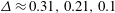
Figure 7. Visualization of the basic symmetric flow regime at
 $\unicode[STIX]{x1D6FD}=300$
,
$\unicode[STIX]{x1D6FD}=300$
,
 $KC=0.5$
using dye. Flow structure at time moments
$KC=0.5$
using dye. Flow structure at time moments
 $t/T-T_{0}$
, where
$t/T-T_{0}$
, where
 $T_{0}=30$
.
$T_{0}=30$
.
5.3 The symmetric flow with attached vortices
Changes in the structure of the flow that occurs during the transition through the boundary of the basic symmetric regime are determined by the range of the oscillation frequencies. At low oscillation frequencies with increasing
 $KC$
a symmetric local vortex structure is developed around the plate (see figures 8, 9
a). Unlike the basic regime, immediately after the reverse near the edges the flow separation occurs with the formation of the attached vortices behind the plate. The formed vortices are developing and growing during a half-period until the plate completely stops and then disappear when the direction of motion changes. In the next half-cycle everything repeats on the other side of the plate. The described flow dynamics can be observed in figure 8. This symmetric regime has a radically different structure of the secondary flow (see figure 9
b), which is divided into inner and outer circulation zones. As can be seen in figure 8, the internal circulation zone prevents the transfer of fluid from the plate to the outer flow region.
$KC$
a symmetric local vortex structure is developed around the plate (see figures 8, 9
a). Unlike the basic regime, immediately after the reverse near the edges the flow separation occurs with the formation of the attached vortices behind the plate. The formed vortices are developing and growing during a half-period until the plate completely stops and then disappear when the direction of motion changes. In the next half-cycle everything repeats on the other side of the plate. The described flow dynamics can be observed in figure 8. This symmetric regime has a radically different structure of the secondary flow (see figure 9
b), which is divided into inner and outer circulation zones. As can be seen in figure 8, the internal circulation zone prevents the transfer of fluid from the plate to the outer flow region.

Figure 8. Visualization of the symmetric flow with attached vortices at
 $\unicode[STIX]{x1D6FD}=20$
,
$\unicode[STIX]{x1D6FD}=20$
,
 $KC=2.5$
using dye. Flow structure at time moments
$KC=2.5$
using dye. Flow structure at time moments
 $t/T-T_{0}$
, where
$t/T-T_{0}$
, where
 $T_{0}=30$
.
$T_{0}=30$
.

Figure 9. The symmetric flow with attached vortices at
 $\unicode[STIX]{x1D6FD}=25$
,
$\unicode[STIX]{x1D6FD}=25$
,
 $KC=2.5$
. (a) Instantaneous streamlines at
$KC=2.5$
. (a) Instantaneous streamlines at
 $t/T-T_{0}=0$
(
$t/T-T_{0}=0$
(
 $T_{0}=30$
), (b) streamlines of the secondary flow.
$T_{0}=30$
), (b) streamlines of the secondary flow.
5.4 The symmetric flow with vertical vortex shedding
The formation of local vortices near the edges of the plate at high oscillation frequencies (
 $\unicode[STIX]{x1D6FD}\geqslant 50$
) occurs in the vicinity of
$\unicode[STIX]{x1D6FD}\geqslant 50$
) occurs in the vicinity of
 $KC=1$
. Unlike the previous symmetrical regime, the vortices that are formed near the edges do not disappear after the reversal, they break away from the plate and move orthogonally to the main stream. The entire cycle from formation to complete dissipation of the vortices takes slightly less than one period. Observing the motion of the dye near the plate (figure 11), it is necessary to pay attention to bright traces propagating from the plate edges along the vertical axis. Colour saturation of the dye indicates a high velocity in these traces. These high-speed flows are formed by secondary streaming. The structure of this streaming is close to that observed in the basic symmetric regime. However, the core of the circulation zones is divided into two parts, which have the same direction of rotation. One of the parts of the divided core is located in the vicinity of the plate, the second is removed to the boundaries of the computational domain.
$KC=1$
. Unlike the previous symmetrical regime, the vortices that are formed near the edges do not disappear after the reversal, they break away from the plate and move orthogonally to the main stream. The entire cycle from formation to complete dissipation of the vortices takes slightly less than one period. Observing the motion of the dye near the plate (figure 11), it is necessary to pay attention to bright traces propagating from the plate edges along the vertical axis. Colour saturation of the dye indicates a high velocity in these traces. These high-speed flows are formed by secondary streaming. The structure of this streaming is close to that observed in the basic symmetric regime. However, the core of the circulation zones is divided into two parts, which have the same direction of rotation. One of the parts of the divided core is located in the vicinity of the plate, the second is removed to the boundaries of the computational domain.

Figure 10. The symmetric flow with vertical vortex shedding at
 $\unicode[STIX]{x1D6FD}=300$
,
$\unicode[STIX]{x1D6FD}=300$
,
 $KC=1$
. (a) Instantaneous streamlines at
$KC=1$
. (a) Instantaneous streamlines at
 $t/T-T_{0}=0$
(
$t/T-T_{0}=0$
(
 $T_{0}=30$
), (b) streamlines of the secondary flow.
$T_{0}=30$
), (b) streamlines of the secondary flow.
Figure 11. Visualization of the symmetric flow with vertical vortex shedding at
 $\unicode[STIX]{x1D6FD}=300$
,
$\unicode[STIX]{x1D6FD}=300$
,
 $KC=1$
using dye. Flow structure at time moments
$KC=1$
using dye. Flow structure at time moments
 $t/T-T_{0}$
, where
$t/T-T_{0}$
, where
 $T_{0}=30$
.
$T_{0}=30$
.
5.5 The hydrodynamic forces acting on the plate in symmetric flow regimes
In symmetric flow regimes only the in-line force
 $F_{x}$
, acting parallel to the oscillation axis, has non-zero values. Variation of
$F_{x}$
, acting parallel to the oscillation axis, has non-zero values. Variation of
 $F_{x}$
with time is presented in figure 12. For small values of dimensionless amplitude the fundamental harmonic is absolutely dominated in the signal
$F_{x}$
with time is presented in figure 12. For small values of dimensionless amplitude the fundamental harmonic is absolutely dominated in the signal
 $F_{x}$
(see figure 12
a). In this case, the main contribution is made by inertial forces proportional to the acceleration of motion. At
$F_{x}$
(see figure 12
a). In this case, the main contribution is made by inertial forces proportional to the acceleration of motion. At
 $KC<0.5$
they give more than 80 % of the total force. With the growth of
$KC<0.5$
they give more than 80 % of the total force. With the growth of
 $KC$
, the contribution of inertial forces decreases, and additional harmonics appear in the signal. In the vicinity of the boundary of the symmetric regimes (see figure 12
b) the portion of inertial forces becomes less than 60 %, the portion of the third harmonic in the signal becomes more than 5 %.
$KC$
, the contribution of inertial forces decreases, and additional harmonics appear in the signal. In the vicinity of the boundary of the symmetric regimes (see figure 12
b) the portion of inertial forces becomes less than 60 %, the portion of the third harmonic in the signal becomes more than 5 %.
In symmetric flow regimes the in-line force is well approximated by the Morison formula (2.8). The corresponding graphs are shown in figure 12. The expansion coefficients were determined for each oscillation period using (2.9). Variation of drag and inertia coefficients over time is shown in figure 13 for the cases
 $KC=0.5,\unicode[STIX]{x1D6FD}=300$
and
$KC=0.5,\unicode[STIX]{x1D6FD}=300$
and
 $KC=1,\unicode[STIX]{x1D6FD}=300$
. After 20 periods the coefficients practically cease to change in time and can be considered as constants. These constants are further used to determine the hydrodynamic coefficients
$KC=1,\unicode[STIX]{x1D6FD}=300$
. After 20 periods the coefficients practically cease to change in time and can be considered as constants. These constants are further used to determine the hydrodynamic coefficients
 $C_{D}$
,
$C_{D}$
,
 $C_{M}$
in symmetric flow regimes.
$C_{M}$
in symmetric flow regimes.

Figure 12. Hydrodynamic forces acting on the plate in symmetric flow regimes. (a)
 $\unicode[STIX]{x1D6FD}=300$
,
$\unicode[STIX]{x1D6FD}=300$
,
 $KC=0.5$
, (b)
$KC=0.5$
, (b)
 $\unicode[STIX]{x1D6FD}=300$
,
$\unicode[STIX]{x1D6FD}=300$
,
 $KC=1$
; ——, results of calculation; ●, Morison approximation.
$KC=1$
; ——, results of calculation; ●, Morison approximation.

Figure 13. The dependence of drag and inertia coefficients on the period of oscillations in symmetric flow regimes: ●,
 $\unicode[STIX]{x1D6FD}=300$
,
$\unicode[STIX]{x1D6FD}=300$
,
 $KC=0.5$
; ▪,
$KC=0.5$
; ▪,
 $\unicode[STIX]{x1D6FD}=300$
,
$\unicode[STIX]{x1D6FD}=300$
,
 $KC=1$
.
$KC=1$
.
5.6 The boundary of symmetric regimes and the mechanisms of symmetry loss
The interaction of vortices with the growth of
 $KC$
at
$KC$
at
 $\unicode[STIX]{x1D6FD}\geqslant 50$
leads to the formation of vortex pairs near the edges (see figure 14
a). Pairs are detached from the edges with a small displacement to the left or right side of the vertical axis of symmetry of the plate (in the first or second half-period, respectively), depending on the initial conditions. The direction of vortex pair shedding remains stable for a large number of periods. This significantly changes the structure of secondary flow around the plate (see figure 14
b). Secondary streams deviate from the vertical axis and take a C-shaped form. As a result, the circulation zones on one side of the plate (in the right half-plane
$\unicode[STIX]{x1D6FD}\geqslant 50$
leads to the formation of vortex pairs near the edges (see figure 14
a). Pairs are detached from the edges with a small displacement to the left or right side of the vertical axis of symmetry of the plate (in the first or second half-period, respectively), depending on the initial conditions. The direction of vortex pair shedding remains stable for a large number of periods. This significantly changes the structure of secondary flow around the plate (see figure 14
b). Secondary streams deviate from the vertical axis and take a C-shaped form. As a result, the circulation zones on one side of the plate (in the right half-plane
 $x>0$
in figure 14
b) are converted into local super-vortices. C-shaped flow retains symmetry with respect to the axis of oscillation. The stability of such a regime (for the considered type of plate) is observed only in a small region in the vicinity of the boundary of the basic symmetric regime. The points corresponding to this regime are marked by unfilled circles in figure 5. With a slight increase of the oscillation amplitude, one of the super-vortices starts to grow stronger than another, as a result, the flow around the plate completely loses horizontal symmetry.
$x>0$
in figure 14
b) are converted into local super-vortices. C-shaped flow retains symmetry with respect to the axis of oscillation. The stability of such a regime (for the considered type of plate) is observed only in a small region in the vicinity of the boundary of the basic symmetric regime. The points corresponding to this regime are marked by unfilled circles in figure 5. With a slight increase of the oscillation amplitude, one of the super-vortices starts to grow stronger than another, as a result, the flow around the plate completely loses horizontal symmetry.

Figure 14. C-shaped flow regime at
 $\unicode[STIX]{x1D6FD}=500$
,
$\unicode[STIX]{x1D6FD}=500$
,
 $KC=1$
. (a) Instantaneous structure of flow obtained using dye; (b) secondary flow.
$KC=1$
. (a) Instantaneous structure of flow obtained using dye; (b) secondary flow.
The mechanism of symmetry loss at low oscillation frequencies (
 $\unicode[STIX]{x1D6FD}<50$
) is different. Vortices forming near the upper and lower edges become unequal in strength (see figure 15
a). This leads to a loss of the horizontal symmetry of the flow. The structure of the motion of the secondary flow thus take the V-shaped form (see figure 15
b). The lifetime of both small and large vortices approximately equal the half-period of the motion. The interactions of vortices formed on different sides of the plate do not occur. The regime with the V-shaped flow structure is also borderline (the corresponding points are denoted by square unfilled markers on the flow regime map in figure 5), with the small increase of
$\unicode[STIX]{x1D6FD}<50$
) is different. Vortices forming near the upper and lower edges become unequal in strength (see figure 15
a). This leads to a loss of the horizontal symmetry of the flow. The structure of the motion of the secondary flow thus take the V-shaped form (see figure 15
b). The lifetime of both small and large vortices approximately equal the half-period of the motion. The interactions of vortices formed on different sides of the plate do not occur. The regime with the V-shaped flow structure is also borderline (the corresponding points are denoted by square unfilled markers on the flow regime map in figure 5), with the small increase of
 $KC$
vortices formed at different half-periods begin to form pairs, this destroys the vertical symmetry of the flow.
$KC$
vortices formed at different half-periods begin to form pairs, this destroys the vertical symmetry of the flow.

Figure 15. V-shaped flow regime at
 $\unicode[STIX]{x1D6FD}=20$
,
$\unicode[STIX]{x1D6FD}=20$
,
 $KC=3.5$
. (a) Instantaneous structure of flow obtained using dye; (b) secondary flow.
$KC=3.5$
. (a) Instantaneous structure of flow obtained using dye; (b) secondary flow.
The comparison of the results with previous studies shows that the obtained estimates of the boundaries of symmetric regimes are close to the experimental results of Shrestha et al. (Reference Shrestha, Ahsan and Aureli2018) (see the boundaries of regimes B and C in figure 5). Note that the authors of this study also distinguish three types of symmetric flows (A, B, C). The absence of a detailed description of the flow structure in the study (Shrestha et al. Reference Shrestha, Ahsan and Aureli2018) does not allow us to produce a complete comparative analysis between the regimes found. According to the localization zones, the A regime corresponds to the basic symmetrical regime, the B regime to the regime with vertical vortex shedding, the C regime to the regime with the attached vortices. The incomplete correspondence between the boundaries of symmetric regimes is most likely explained by the different relative thickness of the plates in the studies. As will be shown later, for thinner samples the boundary of the basic symmetric regime significantly shifts to the region of small amplitudes.
5.7 The one-sided diagonal flow regime
Leaving the zone of borderline regimes, the flow transforms into a regime with a one-sided diagonal vortex shedding, which is observed in the whole range of values of dimensionless oscillation frequency. The flow structure inherits the properties of both V-shaped and C-shaped flows: vortices which are formed near the lower and upper edges are not equal in strength (as in V-shaped flow), vortices which are formed at different half-periods interact with each other, forming vortex pairs (as in C-shaped flow). However, the complete separation of the vortex pair from the plate in this new regime occurs only near the edge, where larger vortices are formed. The vortex pair formed from the small vortices moves along the plate to the opposite edge (where large vortices are formed), where it merges with the vortex formed at the new period of oscillation. The described processes of formation and interaction of vortices can be observed in figure 16, where the visualization of this regime for one period of oscillation is presented.

Figure 16. The one-sided diagonal flow regime at
 $\unicode[STIX]{x1D6FD}=300$
,
$\unicode[STIX]{x1D6FD}=300$
,
 $KC=2.5$
. Flow structure at time moments
$KC=2.5$
. Flow structure at time moments
 $t/T-T_{0}$
, where
$t/T-T_{0}$
, where
 $T_{0}=80$
.
$T_{0}=80$
.
The vortex pairs that are shed from the plate to the outer flow form a super vortex on one side of the plate. The size of this secondary formation rapidly increases at each oscillation period. In figure 16, comparing the flow structure at the beginning of period
 $t/T=T_{0}$
and at the end of the period
$t/T=T_{0}$
and at the end of the period
 $t/T=T_{0}+1$
, one can clearly see the changes of the super-vortex to the left of the plate. As a result of the rapid growth of the vortex, it begins to interact directly with the vortex structure on the plate. This leads to a change of the direction of vortex shedding, or to the displacement of the prevailing vortex to the opposite edge of the plate. In figure 16 to the right of the plate one can see the spot left by the super vortex which was destroyed more than 5 periods ago as a result of a change of the direction of the vortex shedding. Thus, the observed flow regime, which will be referred to hereinafter as a one-sided diagonal flow regime, is not completely periodic.
$t/T=T_{0}+1$
, one can clearly see the changes of the super-vortex to the left of the plate. As a result of the rapid growth of the vortex, it begins to interact directly with the vortex structure on the plate. This leads to a change of the direction of vortex shedding, or to the displacement of the prevailing vortex to the opposite edge of the plate. In figure 16 to the right of the plate one can see the spot left by the super vortex which was destroyed more than 5 periods ago as a result of a change of the direction of the vortex shedding. Thus, the observed flow regime, which will be referred to hereinafter as a one-sided diagonal flow regime, is not completely periodic.
The points corresponding to the one-sided diagonal regime in the parametric plane (
 $\unicode[STIX]{x1D6FD},KC$
) are denoted by triangular markers (see figure 5). Description of the regime with a similar structure can be found in experimental studies of Singh (Reference Singh1979) and Shrestha et al. (Reference Shrestha, Ahsan and Aureli2018). In the work of Shrestha et al. (Reference Shrestha, Ahsan and Aureli2018) it corresponds to the regime D (see figure 5, the boundary of the D regime). Note that Shrestha et al. (Reference Shrestha, Ahsan and Aureli2018) localized this regime at lower amplitudes
$\unicode[STIX]{x1D6FD},KC$
) are denoted by triangular markers (see figure 5). Description of the regime with a similar structure can be found in experimental studies of Singh (Reference Singh1979) and Shrestha et al. (Reference Shrestha, Ahsan and Aureli2018). In the work of Shrestha et al. (Reference Shrestha, Ahsan and Aureli2018) it corresponds to the regime D (see figure 5, the boundary of the D regime). Note that Shrestha et al. (Reference Shrestha, Ahsan and Aureli2018) localized this regime at lower amplitudes
 $KC<1.5$
. Singh (Reference Singh1979) discovered a similar asymmetric regime in the range
$KC<1.5$
. Singh (Reference Singh1979) discovered a similar asymmetric regime in the range
 $3<KC<7$
. Thus, the estimates obtained in this paper lie in the middle between the results of these experimental studies.
$3<KC<7$
. Thus, the estimates obtained in this paper lie in the middle between the results of these experimental studies.
The structure of hydrodynamic forces and the moment acting on the plate in the one-sided diagonal regime is shown in figure 17. As can be seen, an asymmetric flow generates a non-zero lift and torque. As a result of the variation of the flow structure on each period (caused by the development of a super-vortex near the plate) the hydrodynamic influence on the plate also changes with time. The coefficients of the hydrodynamic forces calculated from the Morison approximation also vary from period to period (see figure 18). To determine their characteristic values for a given combination of parameters the averages over the 50 last oscillation periods are calculated.

Figure 17. Hydrodynamic forces and moment acting on the plate in the one-sided diagonal regime at
 $\unicode[STIX]{x1D6FD}=300$
,
$\unicode[STIX]{x1D6FD}=300$
,
 $KC=2.5$
: ——, results of calculation; ●, Morison approximation.
$KC=2.5$
: ——, results of calculation; ●, Morison approximation.

Figure 18. The dependence of the drag and inertia coefficients on the period of oscillations in the one-sided diagonal regime at
 $\unicode[STIX]{x1D6FD}=300$
,
$\unicode[STIX]{x1D6FD}=300$
,
 $KC=2.5$
.
$KC=2.5$
.
5.8 The cyclic diagonal flow regime
The growth of vortices, which occurs with the increase of the oscillation amplitude, leads to the formation of a new flow regime in the vicinity of
 $KC=4$
. Its visualization is shown in figure 19. As in the previous regime, at the moment before the beginning of the reverse motion, large and small vortices are formed near the plate edges (see figure 19 time moment
$KC=4$
. Its visualization is shown in figure 19. As in the previous regime, at the moment before the beginning of the reverse motion, large and small vortices are formed near the plate edges (see figure 19 time moment
 $2/8$
, to the left of the plate). When the plate starts to move in the opposite direction, a large vortex forms a pair with a new vortex that is generated on the other side of the plate. The pair breaks away from the edge of the plate at an angle to the direction of the main oscillatory motion (see figure 19 time moments
$2/8$
, to the left of the plate). When the plate starts to move in the opposite direction, a large vortex forms a pair with a new vortex that is generated on the other side of the plate. The pair breaks away from the edge of the plate at an angle to the direction of the main oscillatory motion (see figure 19 time moments
 $3/8$
–
$3/8$
–
 $5/8$
, to the right of the plate near the upper edge). A small vortex (that was formed near the opposite edge before the reverse) is destroyed after the reversal by the action of a new vortex forming on the other side of the plate. This new vortex in the new half-period grows into the dominant vortex (see figure 19 time moment
$5/8$
, to the right of the plate near the upper edge). A small vortex (that was formed near the opposite edge before the reverse) is destroyed after the reversal by the action of a new vortex forming on the other side of the plate. This new vortex in the new half-period grows into the dominant vortex (see figure 19 time moment
 $6/8$
, to the right of the plate near the lower edge). Thus, in the second half-period the small and large vortices change places with each other. A flow pattern mirrors that observed in the first half-period (see figure 19, time moments
$6/8$
, to the right of the plate near the lower edge). Thus, in the second half-period the small and large vortices change places with each other. A flow pattern mirrors that observed in the first half-period (see figure 19, time moments
 $6/8$
–1, 0–
$6/8$
–1, 0–
 $1/8$
). Vortex pair detachment in this regime occurs alternately from the opposite edges, detached pairs move away from the plate in different directions at an angle to the axis of oscillation, forming two vortex streets. Further, this flow regime will be called the cyclic diagonal regime.
$1/8$
). Vortex pair detachment in this regime occurs alternately from the opposite edges, detached pairs move away from the plate in different directions at an angle to the axis of oscillation, forming two vortex streets. Further, this flow regime will be called the cyclic diagonal regime.

Figure 19. The stable cyclic diagonal regime;
 $\unicode[STIX]{x1D6FD}=300$
,
$\unicode[STIX]{x1D6FD}=300$
,
 $KC=6$
. Flow structure at time moments
$KC=6$
. Flow structure at time moments
 $t/T-T_{0}$
, where
$t/T-T_{0}$
, where
 $T_{0}=56$
.
$T_{0}=56$
.

Figure 20. Hydrodynamic forces and moment acting on the plate in the cyclic diagonal regime at
 $\unicode[STIX]{x1D6FD}=300$
,
$\unicode[STIX]{x1D6FD}=300$
,
 $KC=6$
; ——, results of calculation; ●, Morison approximation.
$KC=6$
; ——, results of calculation; ●, Morison approximation.

Figure 21. The dependence of the drag and inertia coefficients on the period of the oscillations in the cyclic diagonal regime at
 $\unicode[STIX]{x1D6FD}=300$
,
$\unicode[STIX]{x1D6FD}=300$
,
 $KC=6$
.
$KC=6$
.
In the range
 $4\leqslant KC<6$
(see the flow regime map, unfilled diamond markers) the flow starts to transform from the one-sided diagonal regime to the cyclic diagonal regime. The one-sided diagonal flow regime, after several oscillation periods, is switched to a diagonal flow regime, then the flow pattern is again changed to one-sided and so on. We will call this flow behaviour the intermittent diagonal regime. At
$4\leqslant KC<6$
(see the flow regime map, unfilled diamond markers) the flow starts to transform from the one-sided diagonal regime to the cyclic diagonal regime. The one-sided diagonal flow regime, after several oscillation periods, is switched to a diagonal flow regime, then the flow pattern is again changed to one-sided and so on. We will call this flow behaviour the intermittent diagonal regime. At
 $KC\geqslant 6$
the cyclic diagonal regime is fully stabilized (on the flow regime map the cyclic flow is indicated by filled diamond markers). The localized cyclic diagonal regime corresponds exactly to the ‘cyclic flow regime’ described by Singh (Reference Singh1979). The stable diagonal vortex shedding in the experiments (Singh Reference Singh1979) was observed at
$KC\geqslant 6$
the cyclic diagonal regime is fully stabilized (on the flow regime map the cyclic flow is indicated by filled diamond markers). The localized cyclic diagonal regime corresponds exactly to the ‘cyclic flow regime’ described by Singh (Reference Singh1979). The stable diagonal vortex shedding in the experiments (Singh Reference Singh1979) was observed at
 $KC>7$
. Differences in the determination of the boundaries of regimes between numerical and experimental data can be explained by additional perturbations in the experiments.
$KC>7$
. Differences in the determination of the boundaries of regimes between numerical and experimental data can be explained by additional perturbations in the experiments.
The structure of the hydrodynamic forces and the moment acting on the plate in the cyclic diagonal flow regime is shown in figure 20. The in-line component of the force in this regime is almost completely determined by the drag force. For the case presented in figure 20 the contribution of the drag is more than 94 %. The periodic detachment of vortices from the edges of the plate also creates a torque, which predominant frequency is twice as high as the fundamental frequency of oscillations.
The coefficients
 $C_{D}$
,
$C_{D}$
,
 $C_{M}$
computed at each period of oscillation are shown in figure 21. As can be seen, the final stabilization of hydrodynamic coefficients (when they take constant values) occurs after approximately 60 oscillation periods, that is much longer than the stabilization time of symmetric regimes. The final constant values are further used to determine the hydrodynamic coefficients
$C_{M}$
computed at each period of oscillation are shown in figure 21. As can be seen, the final stabilization of hydrodynamic coefficients (when they take constant values) occurs after approximately 60 oscillation periods, that is much longer than the stabilization time of symmetric regimes. The final constant values are further used to determine the hydrodynamic coefficients
 $C_{D}$
,
$C_{D}$
,
 $C_{M}$
of the cyclic diagonal flow regime. The stabilization of the inertia coefficient occurs much faster than stabilization of the drag coefficient. After the fifth period
$C_{M}$
of the cyclic diagonal flow regime. The stabilization of the inertia coefficient occurs much faster than stabilization of the drag coefficient. After the fifth period
 $C_{M}$
is determined with a relative error of 5 %. To achieve the same accuracy in the calculation of
$C_{M}$
is determined with a relative error of 5 %. To achieve the same accuracy in the calculation of
 $C_{D}$
it is necessary to employ at least 12 periods of oscillation.
$C_{D}$
it is necessary to employ at least 12 periods of oscillation.
6 The drag and added mass coefficients
6.1 The influence of the oscillation parameters on added mass and drag coefficients
In the first paragraph of this section we present the dependences of the coefficients of inertia and drag forces on the oscillation parameters for the plate with chamfered edges (II type) and a relative thickness
 $\unicode[STIX]{x1D6E5}=0.1$
. The dependences of the drag coefficient
$\unicode[STIX]{x1D6E5}=0.1$
. The dependences of the drag coefficient
 $C_{D}$
on dimensionless amplitude
$C_{D}$
on dimensionless amplitude
 $KC$
for different values of dimensionless frequency
$KC$
for different values of dimensionless frequency
 $\unicode[STIX]{x1D6FD}$
are shown in figure 22. All plotted curves have a typical S form. In the range of low values of
$\unicode[STIX]{x1D6FD}$
are shown in figure 22. All plotted curves have a typical S form. In the range of low values of
 $KC$
, where the flow near the plate is in the basic symmetric regime, the behaviour of
$KC$
, where the flow near the plate is in the basic symmetric regime, the behaviour of
 $C_{D}(KC,\unicode[STIX]{x1D6FD})$
coincides well with the ‘Stokes’ approximation of the drag forces (see Aureli et al.
Reference Aureli, Porfiri and Basaran2012)
$C_{D}(KC,\unicode[STIX]{x1D6FD})$
coincides well with the ‘Stokes’ approximation of the drag forces (see Aureli et al.
Reference Aureli, Porfiri and Basaran2012)
 $$\begin{eqnarray}\displaystyle KC\rightarrow 0:\quad C_{D}=28.97/(KC\sqrt{\unicode[STIX]{x1D6FD}}). & & \displaystyle\end{eqnarray}$$
The range of applicability of the linear theory depends on the parameter
 $\unicode[STIX]{x1D6FD}$
. After the ‘Stokes’ range, the phase of the growth of the drag coefficient begins. This phase is associated with the development of nonlinear processes in the flow. Note that the flow regime does not change. The growth phase ends near the stability boundary of the basic symmetric regime, after that a further decrease of the drag coefficient begins. For the large values of
$\unicode[STIX]{x1D6FD}$
. After the ‘Stokes’ range, the phase of the growth of the drag coefficient begins. This phase is associated with the development of nonlinear processes in the flow. Note that the flow regime does not change. The growth phase ends near the stability boundary of the basic symmetric regime, after that a further decrease of the drag coefficient begins. For the large values of
 $KC$
, where the flow is in of the cyclic diagonal regime, the curves
$KC$
, where the flow is in of the cyclic diagonal regime, the curves
 $C_{D}(KC)$
for different values of
$C_{D}(KC)$
for different values of
 $\unicode[STIX]{x1D6FD}$
have almost the same behaviour. The variation of the coefficient in this zone is well described by the approximation proposed by Egorov et al. (Reference Egorov, Kamalutdinov and Nuriev2018)
$\unicode[STIX]{x1D6FD}$
have almost the same behaviour. The variation of the coefficient in this zone is well described by the approximation proposed by Egorov et al. (Reference Egorov, Kamalutdinov and Nuriev2018)
 $$\begin{eqnarray}\displaystyle KC>6:\quad C_{D}\approx 4.427(KC/2\unicode[STIX]{x03C0})^{-0.58}. & & \displaystyle\end{eqnarray}$$

Figure 22. Drag coefficient
 $C_{D}$
as a function of
$C_{D}$
as a function of
 $KC$
for the plate of type II with
$KC$
for the plate of type II with
 $\unicode[STIX]{x1D6E5}=0.1$
. (a) Graphs for different values of
$\unicode[STIX]{x1D6E5}=0.1$
. (a) Graphs for different values of
 $\unicode[STIX]{x1D6FD}$
, (b) comparison with the results of other studies.
$\unicode[STIX]{x1D6FD}$
, (b) comparison with the results of other studies.

Figure 23. Inertia coefficient
 $C_{M}$
as a function of
$C_{M}$
as a function of
 $KC$
for the plate of type II with
$KC$
for the plate of type II with
 $\unicode[STIX]{x1D6E5}=0.1$
. (a) Graphs for different values of
$\unicode[STIX]{x1D6E5}=0.1$
. (a) Graphs for different values of
 $\unicode[STIX]{x1D6FD}$
, (b) comparison with the results of other studies.
$\unicode[STIX]{x1D6FD}$
, (b) comparison with the results of other studies.
The dependences of the inertia coefficient
 $C_{M}$
on
$C_{M}$
on
 $KC$
for different values of
$KC$
for different values of
 $\unicode[STIX]{x1D6FD}$
are shown in figure 23. As can be seen, at low amplitudes of the oscillations in the basic symmetric flow regime
$\unicode[STIX]{x1D6FD}$
are shown in figure 23. As can be seen, at low amplitudes of the oscillations in the basic symmetric flow regime
 $C_{M}$
values for fixed
$C_{M}$
values for fixed
 $\unicode[STIX]{x1D6FD}$
are almost constant. The behaviour of
$\unicode[STIX]{x1D6FD}$
are almost constant. The behaviour of
 $C_{M}$
in this range is well described by the ‘Stokes’ approximation (Aureli et al.
Reference Aureli, Porfiri and Basaran2012)
$C_{M}$
in this range is well described by the ‘Stokes’ approximation (Aureli et al.
Reference Aureli, Porfiri and Basaran2012)
 $$\begin{eqnarray}\displaystyle KC\rightarrow 0:\quad C_{M}=1.02+2.45\unicode[STIX]{x1D6FD}^{-1/2}. & & \displaystyle\end{eqnarray}$$
After the loss of stability of the basic symmetric flow regime, the phase of growth of the inertia coefficient begins, which is replaced by a phase of decrease in the vicinity of
 $KC=6$
, where a diagonal flow regime is stabilized.
$KC=6$
, where a diagonal flow regime is stabilized.
The presented data for the plate with chamfered edges agrees well with the experimental estimates of
 $C_{D}$
and
$C_{D}$
and
 $C_{M}$
for samples with similar geometric characteristics that were obtained by Singh (Reference Singh1979), Bearman et al. (Reference Bearman, Downie, Graham and Obasaju1985), Egorov et al. (Reference Egorov, Kamalutdinov and Nuriev2018). Moreover, in the whole range of parameters we get quite a good agreement between our numerical results and the empirical formula proposed in Egorov et al. (Reference Egorov, Kamalutdinov and Nuriev2018)
$C_{M}$
for samples with similar geometric characteristics that were obtained by Singh (Reference Singh1979), Bearman et al. (Reference Bearman, Downie, Graham and Obasaju1985), Egorov et al. (Reference Egorov, Kamalutdinov and Nuriev2018). Moreover, in the whole range of parameters we get quite a good agreement between our numerical results and the empirical formula proposed in Egorov et al. (Reference Egorov, Kamalutdinov and Nuriev2018)
 $$\begin{eqnarray}\displaystyle C_{D}(KC,\unicode[STIX]{x1D6FD})={\displaystyle \frac{28.97}{KC\sqrt{\unicode[STIX]{x1D6FD}}}}+0.171\left({\displaystyle \frac{KC}{2\unicode[STIX]{x03C0}}}\right)^{a-0.58}{\displaystyle \frac{\left(a+3.087+25.8\left({\displaystyle \frac{KC}{2\unicode[STIX]{x03C0}}}\right)^{a}\right)}{\left(0.12+\left({\displaystyle \frac{KC}{2\unicode[STIX]{x03C0}}}\right)^{a}\right)^{2}}}, & & \displaystyle\end{eqnarray}$$
where
 $a=1.03+16.61\unicode[STIX]{x1D6FD}^{-0.627}$
.
$a=1.03+16.61\unicode[STIX]{x1D6FD}^{-0.627}$
.
Comparing with other data shown in figure 22, one could note the presence of a number of results (e.g. Keulegan & Carpenter Reference Keulegan and Carpenter1958; Egorov et al. Reference Egorov, Kamalutdinov, Nuriev and Paimushin2014; Tafuni & Sahin Reference Tafuni and Sahin2015) which give radically different estimates of the hydrodynamic coefficients. These results were mainly obtained for plates with slightly different geometric characteristics. Therefore, it is important to identify how the shape of the samples influences the hydrodynamic forces.
6.2 The effect of the shape of the plate edges
Firstly we evaluate the hydrodynamic influence on the samples with the same thickness
 $\unicode[STIX]{x1D6E5}=0.1$
, but with different shapes of edges. The results of calculations of
$\unicode[STIX]{x1D6E5}=0.1$
, but with different shapes of edges. The results of calculations of
 $C_{D}$
and
$C_{D}$
and
 $C_{M}$
for plates of three different types are shown in figure 24. The structure of the flow and the boundaries of the flow regimes for the compared samples are similar. However, the values of the hydrodynamic coefficients in the area of high and moderate amplitude of oscillations have a visible difference. The results of the measurements of
$C_{M}$
for plates of three different types are shown in figure 24. The structure of the flow and the boundaries of the flow regimes for the compared samples are similar. However, the values of the hydrodynamic coefficients in the area of high and moderate amplitude of oscillations have a visible difference. The results of the measurements of
 $C_{D}$
for a plate with rectangular edges and a plate with a small corner radius
$C_{D}$
for a plate with rectangular edges and a plate with a small corner radius
 $R=0.1$
are on average 13 % higher than the values of
$R=0.1$
are on average 13 % higher than the values of
 $C_{D}$
obtained for a fully rounded plate (
$C_{D}$
obtained for a fully rounded plate (
 $R=0.5$
) and plate with chamfered edges at
$R=0.5$
) and plate with chamfered edges at
 $KC>3$
.
$KC>3$
.

Figure 24. Force coefficients
 $C_{D}$
and
$C_{D}$
and
 $C_{M}$
as a function of
$C_{M}$
as a function of
 $KC$
for
$KC$
for
 $\unicode[STIX]{x1D6FD}=50$
obtained for plates of different types with relative thickness of
$\unicode[STIX]{x1D6FD}=50$
obtained for plates of different types with relative thickness of
 $\unicode[STIX]{x1D6E5}=0.1$
.
$\unicode[STIX]{x1D6E5}=0.1$
.
To find the reasons for these differences, which occur after minor changes of the geometry of the samples, we compare the flow structure around plates of different cross-sections at
 $KC=7$
and measure the pressure distribution over the surface of the plates.
$KC=7$
and measure the pressure distribution over the surface of the plates.
As can be seen in figure 25, the flows around plates of type I and type II in general are very similar. In particular, the structure, the size and the position of vortex pairs formed near the plates remain identical. However, in the vicinity of the edges of the plates there are markable differences in the flow associated with the shift of the flow separation points: for the plate with chamfered edges the separation points are at the vertices of the sharp angles, for the plate with a rectangular cross-section the separation occurs at the vertices of the right angles at the windward side. The positions of the separation points for the plates of different types are shown in figure 26.

Figure 25. Comparison of flow structure and pressure distribution over the surface of plates at
 $\unicode[STIX]{x1D6FD}=55,KC=7$
between a plate of type II (instantaneous flow patterns in the left column, grey lines on the pressure distribution plot) and of type I (instantaneous flow patterns in the right column, black lines on the pressure distribution plot) with the same relative thickness
$\unicode[STIX]{x1D6FD}=55,KC=7$
between a plate of type II (instantaneous flow patterns in the left column, grey lines on the pressure distribution plot) and of type I (instantaneous flow patterns in the right column, black lines on the pressure distribution plot) with the same relative thickness
 $\unicode[STIX]{x1D6E5}=0.1$
for the time moments (from top to bottom)
$\unicode[STIX]{x1D6E5}=0.1$
for the time moments (from top to bottom)
 $t/T-T_{0}=0,1/7,2/7,3/7$
. The dotted lines on the pressure distribution plot correspond to the left side of the plates (
$t/T-T_{0}=0,1/7,2/7,3/7$
. The dotted lines on the pressure distribution plot correspond to the left side of the plates (
 $x<0$
), the solid lines correspond to the right side of the plates (
$x<0$
), the solid lines correspond to the right side of the plates (
 $x>0$
).
$x>0$
).

Figure 26. Flow separation from the edges of plates of different shapes: (a) type II,
 $\unicode[STIX]{x1D6E5}=0.1,\unicode[STIX]{x1D6FC}=60^{\circ }$
; (b) type I,
$\unicode[STIX]{x1D6E5}=0.1,\unicode[STIX]{x1D6FC}=60^{\circ }$
; (b) type I,
 $\unicode[STIX]{x1D6E5}=0.1$
; (c) type III,
$\unicode[STIX]{x1D6E5}=0.1$
; (c) type III,
 $\unicode[STIX]{x1D6E5}=0.1,R=0.1$
; (d) type III,
$\unicode[STIX]{x1D6E5}=0.1,R=0.1$
; (d) type III,
 $\unicode[STIX]{x1D6E5}=0.1,R=0.5$
.
$\unicode[STIX]{x1D6E5}=0.1,R=0.5$
.
The analysis of the pressure distribution over the plate surface allows us to estimate the significance of the observed differences. As can be seen from the presented pressure distribution plots (see figure 25), in almost all phases of the flow development the difference between the pressure on the right and left sides of the plate of type II in the vicinity of the edges is less than that of the plate of type I. Since at these values of the amplitude the pressure force gives the main contribution to the total hydrodynamic force, the observed differences fully explain the decrease in the resulting aerodynamic drag of the plate with chamfered edges.
6.3 The effect of the relative thickness of the plate
Significant differences are found when comparing the hydrodynamic coefficients calculated for plates with different thicknesses (see figure 27) for
 $\unicode[STIX]{x1D6FD}\geqslant 50$
. The maximum relative deviation (about 90 %) between the values of
$\unicode[STIX]{x1D6FD}\geqslant 50$
. The maximum relative deviation (about 90 %) between the values of
 $C_{D}$
is observed for the infinitely thin plate and plates with relative thickness
$C_{D}$
is observed for the infinitely thin plate and plates with relative thickness
 $\unicode[STIX]{x1D6E5}=0.1,0.25$
in the range
$\unicode[STIX]{x1D6E5}=0.1,0.25$
in the range
 $0.2<KC<1$
.
$0.2<KC<1$
.

Figure 27. Force coefficients
 $C_{D}$
and
$C_{D}$
and
 $C_{M}$
as a function of
$C_{M}$
as a function of
 $KC$
for
$KC$
for
 $\unicode[STIX]{x1D6FD}=200$
obtained for plates of type II with relative thicknesses of
$\unicode[STIX]{x1D6FD}=200$
obtained for plates of type II with relative thicknesses of
 $\unicode[STIX]{x1D6E5}=0,0.1,0.25$
.
$\unicode[STIX]{x1D6E5}=0,0.1,0.25$
.
Such significant differences can be explained by various flow regimes observed in the specified range for the plates with different thicknesses. The boundary value of
 $KC$
at which the transition from the basic symmetric regime to the regime with the vertical shedding of vortices happens for the plates with relative thickness
$KC$
at which the transition from the basic symmetric regime to the regime with the vertical shedding of vortices happens for the plates with relative thickness
 $\unicode[STIX]{x1D6E5}=0.1,0.25$
is practically the same and approximately equal to
$\unicode[STIX]{x1D6E5}=0.1,0.25$
is practically the same and approximately equal to
 $KC=1$
(see figure 5). For the infinitely thin plate this transition occurs much earlier: for
$KC=1$
(see figure 5). For the infinitely thin plate this transition occurs much earlier: for
 $\unicode[STIX]{x1D6FD}=200$
the boundary is below
$\unicode[STIX]{x1D6FD}=200$
the boundary is below
 $KC=0.2$
.
$KC=0.2$
.
The results of measurements of the pressure distribution on the surface of an infinitely thin plate in the regime with the vertical shedding of vortices and on the plate with thickness
 $\unicode[STIX]{x1D6E5}=0.1$
in the basic symmetric regime for the same values of the oscillation parameters
$\unicode[STIX]{x1D6E5}=0.1$
in the basic symmetric regime for the same values of the oscillation parameters
 $\unicode[STIX]{x1D6FD}=200,KC=0.8$
are shown in figure 28. As can be seen, the difference between the pressure on the right and left sides on an infinitely thin plate is larger at all phases of motion.
$\unicode[STIX]{x1D6FD}=200,KC=0.8$
are shown in figure 28. As can be seen, the difference between the pressure on the right and left sides on an infinitely thin plate is larger at all phases of motion.

Figure 28. The distribution of the true pressure over the surfaces of an infinitely thin plate (black lines) and a plate of type II with a thickness of
 $\unicode[STIX]{x1D6E5}=0.1$
(grey lines) for the oscillation parameters
$\unicode[STIX]{x1D6E5}=0.1$
(grey lines) for the oscillation parameters
 $\unicode[STIX]{x1D6FD}=200,KC=0.8$
. Time moments
$\unicode[STIX]{x1D6FD}=200,KC=0.8$
. Time moments
 $t/T-T_{0}$
: (a)
$t/T-T_{0}$
: (a)
 $0$
, (b)
$0$
, (b)
 $1/8$
, (c)
$1/8$
, (c)
 $2/8$
, (d)
$2/8$
, (d)
 $3/8$
. Dotted lines correspond to the left side of the plates (
$3/8$
. Dotted lines correspond to the left side of the plates (
 $x<0$
), solid lines to the right side of the plates (
$x<0$
), solid lines to the right side of the plates (
 $x>0$
).
$x>0$
).
Note that the data obtained for an infinitely thin plate coincide well with the experimental results of Keulegan & Carpenter (Reference Keulegan and Carpenter1958) and numerical data of Egorov et al. (Reference Egorov, Kamalutdinov, Nuriev and Paimushin2014), Tafuni & Sahin (Reference Tafuni and Sahin2015). Thus, the presented results give an explanation of the differences of the
 $C_{D}$
estimates that were obtained in different studies.
$C_{D}$
estimates that were obtained in different studies.
7 Conclusion
The data collected in the work allow us to fill in the large gaps indicated at the beginning of the paper related to the problem of interaction of oscillating plates with a fluid. The obtained results make it possible to classify practically all flow regimes around the plate in the range
 $20\leqslant \unicode[STIX]{x1D6FD}\leqslant 500,0<KC\leqslant 10$
, which were discovered earlier in various experimental studies. Thus the one-sided diagonal regime and the cyclic diagonal regime formed near the plates at moderate and high oscillation amplitudes, that were discovered earlier in the experiments by Keulegan & Carpenter (Reference Keulegan and Carpenter1958) and Singh (Reference Singh1979), were simulated and described in detail for the first time. In the range of low amplitudes of oscillation three symmetric flow regimes, localized earlier in the experiments by Shrestha et al. (Reference Shrestha, Ahsan and Aureli2018), were simulated and studied. We also discovered for the first time the V-shaped and C-shaped transition regimes appearing in narrow parametric regions along the stability boundary of symmetric flow regimes.
$20\leqslant \unicode[STIX]{x1D6FD}\leqslant 500,0<KC\leqslant 10$
, which were discovered earlier in various experimental studies. Thus the one-sided diagonal regime and the cyclic diagonal regime formed near the plates at moderate and high oscillation amplitudes, that were discovered earlier in the experiments by Keulegan & Carpenter (Reference Keulegan and Carpenter1958) and Singh (Reference Singh1979), were simulated and described in detail for the first time. In the range of low amplitudes of oscillation three symmetric flow regimes, localized earlier in the experiments by Shrestha et al. (Reference Shrestha, Ahsan and Aureli2018), were simulated and studied. We also discovered for the first time the V-shaped and C-shaped transition regimes appearing in narrow parametric regions along the stability boundary of symmetric flow regimes.
Some additional explanations should be provided on the questions about the limits of applicability of the two-dimensional flow model used in the work and about the development of the three-dimensional flow structures. Although previous studies on the development of three-dimensional vortex structures in the flow around oscillating thin long plates are not known to the authors, extensive information is available on the development of three-dimensional flow instability around an oscillating circular cylinder (see Honji Reference Honji1981; Sarpkaya Reference Sarpkaya2002; Nehari, Armenio & Ballio Reference Nehari, Armenio and Ballio2004; Elston, Blackburn & Sheridan Reference Elston, Blackburn and Sheridan2006; An, Cheng & Zhao Reference An, Cheng and Zhao2011; Suthon & Dalton Reference Suthon and Dalton2011; An, Cheng & Zhao Reference An, Cheng and Zhao2015). For a circular cylinder the dependence of the critical value of the Keulegan–Carpenter number
 $KC_{cyl}$
on the parameter
$KC_{cyl}$
on the parameter
 $\unicode[STIX]{x1D6FD}$
at which the flow becomes unstable to three-dimensional perturbations in the range of
$\unicode[STIX]{x1D6FD}$
at which the flow becomes unstable to three-dimensional perturbations in the range of
 $60<\unicode[STIX]{x1D6FD}<1.4\times 10^{6}$
can be approximated by the formula
$60<\unicode[STIX]{x1D6FD}<1.4\times 10^{6}$
can be approximated by the formula
 $KC_{cyl}=12.5\unicode[STIX]{x1D6FD}^{-2/5}$
(proposed by Sarpkaya (Reference Sarpkaya2002)). However, it is more important that the development of three-dimensional structures in the flow (after passing through the stability boundary) in the region of moderate
$KC_{cyl}=12.5\unicode[STIX]{x1D6FD}^{-2/5}$
(proposed by Sarpkaya (Reference Sarpkaya2002)). However, it is more important that the development of three-dimensional structures in the flow (after passing through the stability boundary) in the region of moderate
 $\unicode[STIX]{x1D6FD}$
in a fairly wide range of amplitudes does not lead to a significant redistribution of the kinetic energy of the currents near the cylinder, this is evidenced by the results of three-dimensional modelling (see Nehari et al.
Reference Nehari, Armenio and Ballio2004; An et al.
Reference An, Cheng and Zhao2011, Reference An, Cheng and Zhao2015), and a comparison of the results of two-dimensional models with experiments (see Justesen Reference Justesen1991; Dutsch et al.
Reference Dutsch, Durst, Becker and Lienhart1998). Thus, planar structures remain predominant even after the appearance of three-dimensional flows, which makes it possible to use two-dimensional models for their analysis (albeit with some restrictions). Several three-dimensional calculations in the Appendix of this paper show that for the considered case a similar situation is observed: the two-dimensional model well describes the flow dynamics in planes perpendicular to the plate axis and predicts the forces acting on the plate even after the formation of three-dimensional structures. This is also supported by the consistency of the results of two-dimensional simulations with experiments.
$\unicode[STIX]{x1D6FD}$
in a fairly wide range of amplitudes does not lead to a significant redistribution of the kinetic energy of the currents near the cylinder, this is evidenced by the results of three-dimensional modelling (see Nehari et al.
Reference Nehari, Armenio and Ballio2004; An et al.
Reference An, Cheng and Zhao2011, Reference An, Cheng and Zhao2015), and a comparison of the results of two-dimensional models with experiments (see Justesen Reference Justesen1991; Dutsch et al.
Reference Dutsch, Durst, Becker and Lienhart1998). Thus, planar structures remain predominant even after the appearance of three-dimensional flows, which makes it possible to use two-dimensional models for their analysis (albeit with some restrictions). Several three-dimensional calculations in the Appendix of this paper show that for the considered case a similar situation is observed: the two-dimensional model well describes the flow dynamics in planes perpendicular to the plate axis and predicts the forces acting on the plate even after the formation of three-dimensional structures. This is also supported by the consistency of the results of two-dimensional simulations with experiments.
It should be noted that the most of the observed flow regimes near the plates are very similar to flows formed around a circular cylinder (see the studies of Tatsuno & Bearman (Reference Tatsuno and Bearman1990), Justesen (Reference Justesen1991), Dutsch et al. (Reference Dutsch, Durst, Becker and Lienhart1998), Elston et al. (Reference Elston, Blackburn and Sheridan2006), An et al. (Reference An, Cheng and Zhao2009), Nuriev et al. (Reference Nuriev, Egorov and Zaitseva2018)). Comparing the flows near a circular cylinder and a plate, one can find an almost identical structure of the symmetric regimes observed at small values of
 $KC$
and the diagonal regime formed at high values of the dimensionless oscillation amplitude.
$KC$
and the diagonal regime formed at high values of the dimensionless oscillation amplitude.
In spite of the similarity of the flow regimes observed at identical values of the oscillation parameters, the hydrodynamical influence can be dramatically different even for oscillating bodies with very similar shapes. The results of the present studies have shown that the change of the shape of the plate edges has a noticeable effect on the drag force in flow regimes with intense vortex formation observed at large
 $KC$
. The thickness of the plates significantly affects the hydrodynamic forces in the range of small oscillation amplitudes.
$KC$
. The thickness of the plates significantly affects the hydrodynamic forces in the range of small oscillation amplitudes.
The established dependence between the shape of the oscillating plate and its hydrodynamic drag made it possible to explain the difference between the estimates of
 $C_{D}$
obtained in the classical experimental studies of Keulegan & Carpenter (Reference Keulegan and Carpenter1958) and Singh (Reference Singh1979).
$C_{D}$
obtained in the classical experimental studies of Keulegan & Carpenter (Reference Keulegan and Carpenter1958) and Singh (Reference Singh1979).
Acknowledgements
The research was supported by RSF (research project no. 15-19-10039).
Appendix. A comparison of the results of 2-D and 3-D simulations
In this appendix we consider the results of several three-dimensional calculations and compare them with the results of two-dimensional simulations presented in the main part of the article to determine the importance of three-dimensional effects, which, as will be shown below, may appear in the investigated range of parameters.

Figure 29. The instantaneous flow patterns. (a) C-shaped flow regime at
 $\unicode[STIX]{x1D6FD}=64$
,
$\unicode[STIX]{x1D6FD}=64$
,
 $KC=1$
. Isosurfaces of the
$KC=1$
. Isosurfaces of the
 $z$
component of the vorticity vector
$z$
component of the vorticity vector
 $\unicode[STIX]{x1D6FA}_{z}=\pm [6,4.66,3.33,2,0.34]$
for the time moment
$\unicode[STIX]{x1D6FA}_{z}=\pm [6,4.66,3.33,2,0.34]$
for the time moment
 $t/T=104$
. (b) The one-sided diagonal flow regime at
$t/T=104$
. (b) The one-sided diagonal flow regime at
 $\unicode[STIX]{x1D6FD}=64,KC=2$
. Isosurfaces of the
$\unicode[STIX]{x1D6FD}=64,KC=2$
. Isosurfaces of the
 $z$
component of the vorticity vector
$z$
component of the vorticity vector
 $\unicode[STIX]{x1D6FA}_{z}=\pm [10,8,6,4,3]$
for the time moment
$\unicode[STIX]{x1D6FA}_{z}=\pm [10,8,6,4,3]$
for the time moment
 $t/T=88$
.
$t/T=88$
.

Figure 30. Comparison of the instantaneous flow patterns of two-dimensional flow (a) and span-averaged three-dimensional flow (b) in the
 $xOy$
plane. Scalar field
$xOy$
plane. Scalar field
 $|\unicode[STIX]{x1D6FA}_{z}|$
visualization at the time moment
$|\unicode[STIX]{x1D6FA}_{z}|$
visualization at the time moment
 $t/T=87$
for
$t/T=87$
for
 $\unicode[STIX]{x1D6FD}=64,KC=2$
.
$\unicode[STIX]{x1D6FD}=64,KC=2$
.

Figure 31. Forces acting on the plate in the one-sided diagonal regime for
 $\unicode[STIX]{x1D6FD}=64$
,
$\unicode[STIX]{x1D6FD}=64$
,
 $KC=2$
. Two-dimensional calculation (dotted line), three-dimensional calculation (solid line).
$KC=2$
. Two-dimensional calculation (dotted line), three-dimensional calculation (solid line).
The three-dimensional calculations are performed for a plate of zero thickness at the four points of the parametric plane:
 $\unicode[STIX]{x1D6FD}=64,KC=1,2,7$
and
$\unicode[STIX]{x1D6FD}=64,KC=1,2,7$
and
 $\unicode[STIX]{x1D6FD}=200,KC=7$
. The flow around a plate segment with a length of
$\unicode[STIX]{x1D6FD}=200,KC=7$
. The flow around a plate segment with a length of
 $l_{z}=20$
is considered. The computational domain is bounded by a rectangular parallelepiped, which sides are chosen parallel to the coordinate axes associated with the plate. The size of the computational domain is
$l_{z}=20$
is considered. The computational domain is bounded by a rectangular parallelepiped, which sides are chosen parallel to the coordinate axes associated with the plate. The size of the computational domain is
 $(l_{x},l_{y},l_{z})=(60,40,20)$
. At the ends of the plate segment (
$(l_{x},l_{y},l_{z})=(60,40,20)$
. At the ends of the plate segment (
 $z=0,20$
) periodic boundary conditions are set. The computational mesh consists of
$z=0,20$
) periodic boundary conditions are set. The computational mesh consists of
 $4.5\times 10^{6}$
cells; in the
$4.5\times 10^{6}$
cells; in the
 $xOy$
plane in the vicinity of the body it has the same structure as the
$xOy$
plane in the vicinity of the body it has the same structure as the
 $M_{1}$
mesh (see § 3); in the spanwise direction in the vicinity of the plate it has a uniform spacing equal to
$M_{1}$
mesh (see § 3); in the spanwise direction in the vicinity of the plate it has a uniform spacing equal to
 $0.04$
.
$0.04$
.
The flow at the first examined point
 $\unicode[STIX]{x1D6FD}=64,KC=1$
does not have a three-dimensional structure, so the results of three- and two-dimensional calculations are identical to each other. The instantaneous flow pattern is shown in figure 29, it corresponds to a C-shaped flow which is typical for this range of parameters.
$\unicode[STIX]{x1D6FD}=64,KC=1$
does not have a three-dimensional structure, so the results of three- and two-dimensional calculations are identical to each other. The instantaneous flow pattern is shown in figure 29, it corresponds to a C-shaped flow which is typical for this range of parameters.
The second examined point
 $\unicode[STIX]{x1D6FD}=64,KC=2$
is in the area of the one-sided diagonal flow regime. In the initial time interval (starting from the rest) at this point only a two-dimensional flow structure is formed. At the 20th period in the boundary layer of the plate weak three-dimensional structures become visible. They are similar to the Honji vortices (see, for example, Honji Reference Honji1981, Sarpkaya Reference Sarpkaya2002, Suthon & Dalton Reference Suthon and Dalton2011), which are formed in the boundary layer of a oscillating circular cylinder when a plane flow loses its stability. These three-dimensional (3-D) vortex structures grow over time and interact with each other. The process of intensification of spanwise flow ends closer to the 45th period. The resulting 3-D flow pattern near the plate is shown in figure 29. Omitting a detailed discussion of the three-dimensional processes, we turn to a comparison of the results of two-dimensional and three-dimensional simulations for this case.
$\unicode[STIX]{x1D6FD}=64,KC=2$
is in the area of the one-sided diagonal flow regime. In the initial time interval (starting from the rest) at this point only a two-dimensional flow structure is formed. At the 20th period in the boundary layer of the plate weak three-dimensional structures become visible. They are similar to the Honji vortices (see, for example, Honji Reference Honji1981, Sarpkaya Reference Sarpkaya2002, Suthon & Dalton Reference Suthon and Dalton2011), which are formed in the boundary layer of a oscillating circular cylinder when a plane flow loses its stability. These three-dimensional (3-D) vortex structures grow over time and interact with each other. The process of intensification of spanwise flow ends closer to the 45th period. The resulting 3-D flow pattern near the plate is shown in figure 29. Omitting a detailed discussion of the three-dimensional processes, we turn to a comparison of the results of two-dimensional and three-dimensional simulations for this case.

Figure 32. Cyclic diagonal flow regime at
 $KC=7$
,
$KC=7$
,
 $\unicode[STIX]{x1D6FD}=64$
(a),
$\unicode[STIX]{x1D6FD}=64$
(a),
 $\unicode[STIX]{x1D6FD}=200$
(b). Isosurfaces of the
$\unicode[STIX]{x1D6FD}=200$
(b). Isosurfaces of the
 $z$
component of the vorticity vector
$z$
component of the vorticity vector
 $\unicode[STIX]{x1D6FA}_{z}=\pm [5.55,16.66,27.77,38.88,50]$
for the time moment
$\unicode[STIX]{x1D6FA}_{z}=\pm [5.55,16.66,27.77,38.88,50]$
for the time moment
 $t/T=48$
.
$t/T=48$
.

Figure 33. Comparison of the instantaneous flow patterns of 2-D flow (a) and spanwise-averaged 3-D flow (b) in the
 $xOy$
plane. Scalar field
$xOy$
plane. Scalar field
 $|\unicode[STIX]{x1D6FA}_{z}|$
visualization at the time moment
$|\unicode[STIX]{x1D6FA}_{z}|$
visualization at the time moment
 $t/T=47$
for
$t/T=47$
for
 $\unicode[STIX]{x1D6FD}=64,KC=7$
.
$\unicode[STIX]{x1D6FD}=64,KC=7$
.

Figure 34. Forces acting on the plate in cyclic diagonal flow regime for
 $\unicode[STIX]{x1D6FD}=64$
,
$\unicode[STIX]{x1D6FD}=64$
,
 $KC=7$
(a,b) and
$KC=7$
(a,b) and
 $\unicode[STIX]{x1D6FD}=200,KC=7$
(c,d). Two-dimensional calculations (dotted lines), 3-D calculations (solid lines).
$\unicode[STIX]{x1D6FD}=200,KC=7$
(c,d). Two-dimensional calculations (dotted lines), 3-D calculations (solid lines).
Table 3. The coefficients
 $C_{D}$
and
$C_{D}$
and
 $C_{M}$
for two- and three-dimensional cases.
$C_{M}$
for two- and three-dimensional cases.

In figure 30 the structures of a two-dimensional flow and a spanwise-averaged three-dimensional flow in the
 $xOy$
plane for the same moment of time are compared. As can be seen, the flows in both cases have an identical structure, although the position and size of the vortices are slightly different. As was noted in § 5, the one-sided diagonal regime is not completely periodic, the instantaneous flow depends on the changes that occurred in previous periods. The synchronism of such changes in the 2-D and 3-D calculations is broken. A comparison of the (spanwise-averaged) forces on one period is shown in figure 31. As you can see the variation of the
$xOy$
plane for the same moment of time are compared. As can be seen, the flows in both cases have an identical structure, although the position and size of the vortices are slightly different. As was noted in § 5, the one-sided diagonal regime is not completely periodic, the instantaneous flow depends on the changes that occurred in previous periods. The synchronism of such changes in the 2-D and 3-D calculations is broken. A comparison of the (spanwise-averaged) forces on one period is shown in figure 31. As you can see the variation of the
 $F_{x}$
component is fairly well described in a 2-D simulation. Differences between the average values of the hydrodynamic coefficients
$F_{x}$
component is fairly well described in a 2-D simulation. Differences between the average values of the hydrodynamic coefficients
 $C_{D}$
and
$C_{D}$
and
 $C_{M}$
are less than 3 % (see table 3). Consistency of results for the component
$C_{M}$
are less than 3 % (see table 3). Consistency of results for the component
 $F_{y}$
(see figure 31) is much worse. If we compare the maximum absolute values of the lifting force, the differences between 3-D and 2-D data will be approximately 37 % (see table 3).
$F_{y}$
(see figure 31) is much worse. If we compare the maximum absolute values of the lifting force, the differences between 3-D and 2-D data will be approximately 37 % (see table 3).
The last two points
 $\unicode[STIX]{x1D6FD}=64,KC=7$
and
$\unicode[STIX]{x1D6FD}=64,KC=7$
and
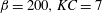 $\unicode[STIX]{x1D6FD}=200,KC=7$
belong to the area of the cyclic diagonal flow regime. As you can see in figure 32 the flows here (as in the previous point) are three-dimensional.
$\unicode[STIX]{x1D6FD}=200,KC=7$
belong to the area of the cyclic diagonal flow regime. As you can see in figure 32 the flows here (as in the previous point) are three-dimensional.
A comparison of the structure of a two-dimensional flow and a spanwise-averaged three-dimensional flow in the
 $xOy$
plane for the same moment of time is shown in figure 33. As can be seen, the two-dimensional model qualitatively predicts the dynamics of the flow. The quantitative results of the calculation of the in-line component of force
$xOy$
plane for the same moment of time is shown in figure 33. As can be seen, the two-dimensional model qualitatively predicts the dynamics of the flow. The quantitative results of the calculation of the in-line component of force
 $F_{x}$
(see figure 34), as well as the values of hydrodynamic coefficients determined from them (see table 3) agree well. The lift force values (see figure 34 and the data in table 3) calculated in 2-D and 3-D cases again have visible differences. These errors of the two-dimensional model are not critical, since
$F_{x}$
(see figure 34), as well as the values of hydrodynamic coefficients determined from them (see table 3) agree well. The lift force values (see figure 34 and the data in table 3) calculated in 2-D and 3-D cases again have visible differences. These errors of the two-dimensional model are not critical, since
 $F_{y}$
has a very weak effect on the plate.
$F_{y}$
has a very weak effect on the plate.


