


1. Introduction
The instability that occurs at the interface between two fluids of different densities due to the acceleration of a shock wave is referred to as the Richtmyer–Meshkov (RM) instability (Richtmyer Reference Richtmyer1960; Meshkov Reference Meshkov1969). The RM instability is usually recognized as the impulsive counterpart to the Rayleigh–Taylor (RT) instability (Rayleigh Reference Rayleigh1883; Taylor Reference Taylor1950) that occurs when the heavy fluid is persistently accelerated by the light fluid. The evolution of the RM instability can be of particular importance in implosion dynamics of inertial-confinement fusion (Betti & Hurricane Reference Betti and Hurricane2016) and explosion dynamics of supernova (Kane, Drake & Remington Reference Kane, Drake and Remington1999), which are characterised by converging/diverging geometries. In such circumstances, the shock wave and fluid interface are subject to geometrical convergence/divergence, which is known as the Bell–Plesset (BP) effect (Bell Reference Bell1951; Plesset Reference Plesset1954), and are radially accelerated or decelerated during their propagations. The resultant RT stabilizing or destabilizing effects (Lombardini, Pullin & Meiron Reference Lombardini, Pullin and Meiron2014a) as well as the fluid compressibility (Zhang, Deng & Guo Reference Zhang, Deng and Guo2018) and a second shock-interface interaction (reshock) (Schilling, Latini & Don Reference Schilling, Latini and Don2007) further reinforce the complexity of the RM instability development and present significant challenges for modelling and prediction of the perturbation growth. The RM instability and induced turbulent mixing flow have attracted much attention in the past half century (Rupert Reference Rupert1992; Brouillette Reference Brouillette2002; Ranjan, Oakley & Bonazza Reference Ranjan, Oakley and Bonazza2011; Zhou Reference Zhou2017a,Reference Zhoub). Previous research has mainly focused on the planar geometry both experimentally (Dimonte, Frerking & Schneider Reference Dimonte, Frerking and Schneider1995; Jones & Jacobs Reference Jones and Jacobs1997; Sadot et al. Reference Sadot, Erez, Alon, Oron, Levin, Erez, Ben-Dor and Shvarts1998; Jacobs & Krivets Reference Jacobs and Krivets2005; Jourdan & Houas Reference Jourdan and Houas2005; Mariani et al. Reference Mariani, Vandenboomgaerde, Jourdan, Souffland and Houas2008) and numerically (Thornber & Zhou Reference Thornber and Zhou2012; Tritschler et al. Reference Tritschler, Olson, Lele, Hickel, Hu and Adams2014; Liu & Xiao Reference Liu and Xiao2016; Groom & Thornber Reference Groom and Thornber2019), not only because of the clarity of the physical image in the planar geometry but because of the difficulties encountered in the experimental set-up and numerical treatment of the shock wave and initial interface in the converging case.
An early attempt to conduct experimental measurements on the RM instability in the converging geometry was made by Fincke et al. (Reference Fincke, Lanier, Batha, Hueckstaedt, Magelssen, Rothman, Parker and Horsfield2004), who studied the growth patterns of single-mode perturbations at the epoxy/aluminium interface in a laser-driven cylindrical target. Hosseini & Takayama (Reference Hosseini and Takayama2005) were among the first to implement an experimental visualization of the cylindrical RM instability induced by cylindrical shock wave propagation across gas bubbles in an annular coaxial vertical shock tube. Si, Zhai & Luo (Reference Si, Zhai and Luo2014) investigated the cylindrical RM instability in a horizontal shock tube with a specially designed test section. Luo et al. (Reference Luo, Zhang, Ding, Si, Yang, Zhai and Wen2018) studied the long-term RT stabilizing effect in the RM instability in a similar shock tube. Using a gas lensing technique, Biamino et al. (Reference Biamino, Jourdan, Mariani, Houas, Vandenboomgaerde and Souffland2015) studied the converging RM instability in a wedge that was mounted to a conventional shock tube Dimotakis & Samtaney (Reference Dimotakis and Samtaney2006). Recently, a semiannular shock tube was designed with an improved formation technique for the initial gaseous interface (Luo et al. Reference Luo, Ding, Wang, Zhai and Si2015), which was utilized to study the converging RM instability at a single-mode air-SF $_6$ interface (Ding et al. Reference Ding, Si, Yang, Lu, Zhai and Luo2017), and provided early quantitative shock tube results of the perturbation and shock evolutions before and after reshock.
In view of the lack of quantitative experimental measurements, most previous numerical studies have explored the evolution law of the RM instability in two-dimensional (2-D) azimuthal or axisymmetric geometries (Zhang & Graham Reference Zhang and Graham1997; Glimm et al. Reference Glimm, Grove, Zhang and Dutta2002; Zheng, Lee & Winoto Reference Zheng, Lee and Winoto2008), and in three-dimensional (3-D) cylindrical and spherical geometries (Dutta et al. Reference Dutta, Glimma, Grove, Sharp and Zhang2004; Youngs & Williams Reference Youngs and Williams2008; Lombardini & Pullin Reference Lombardini and Pullin2009; Lombardini et al. Reference Lombardini, Pullin and Meiron2014a; Lombardini, Pullin & Meiron Reference Lombardini, Pullin and Meiron2014b; Wu, Liu & Xiao Reference Wu, Liu and Xiao2019). The focus of such research has mainly been on the asymptotic growth rate or the initial condition effects of turbulent mixing after reshock, with little attention given to the early linear and weak nonlinear stages of perturbation growth before reshock. More recently, Zhai et al. (Reference Zhai, Zhang, Zhang, Ding and Wen2019) numerically investigated the RT effects on the phase inversion before reshock and the results compared well with their experimental data (Luo et al. Reference Luo, Zhang, Ding, Si, Yang, Zhai and Wen2018; Ding et al. Reference Ding, Si, Yang, Lu, Zhai and Luo2017).
In this paper, direct numerical simulation (DNS) of the 2-D cylindrical RM instability at a single-mode air-SF $_6$ interface is implemented in accordance with the experimental set-up reported by Lei et al. (Reference Lei, Ding, Si, Zhai and Luo2017) and Lei (Reference Lei2017). The aim is to present a methodology for numerical settings towards simulation-experiment comparison, and establish an improved model for the evolution of initial perturbations in the converging RM instability before reshock.
2. Numerical methods and simulation settings
The RM instability and induced mixing flow are governed by the multicomponent Navier–Stokes equations, equations of mass fractions, and equation of state, which take the forms
 \begin{gather} \frac{\partial \rho}{\partial t}+\boldsymbol{\nabla} \boldsymbol{\cdot} (\rho \boldsymbol{u})=0, \end{gather}
 \begin{gather}\frac{\partial \rho \boldsymbol{u}}{\partial t}+\boldsymbol{\nabla} \boldsymbol{\cdot} (\rho \boldsymbol{u} \boldsymbol{u}+p\boldsymbol{\delta}-\boldsymbol{\tau})=0, \end{gather}
 \begin{gather}\frac{\partial E}{\partial t}+\boldsymbol{\nabla} \boldsymbol{\cdot} (E \boldsymbol{u}+(p\boldsymbol{\delta}-\boldsymbol{\tau})\boldsymbol{\cdot} \boldsymbol{u}+\boldsymbol{q_{c}}+\boldsymbol{q_{d}})=0, \end{gather}
 \begin{gather}\frac{\partial \rho Y_{i}}{\partial t}+\boldsymbol{\nabla} \boldsymbol{\cdot} (\rho \boldsymbol{u} Y_{i})+\boldsymbol{\nabla} \boldsymbol{\cdot} \boldsymbol{J_{i}}=0, \quad i=1,2, \end{gather}
 \begin{gather}p=\frac{\rho TR}{\bar{M}}=(\bar{\gamma}-1)\rho e. \end{gather}
Here,  $\rho$ is the mixture density,
  $\boldsymbol {u}=(u,v,w)$ is the velocity vector,
  $p$ is the static pressure,
  $T$ is the temperature and
  $Y_i$ is the mass fraction of species
  $i$ (
$i$ ( $i=1,2$). The symbol
  $\boldsymbol {\nabla }$ denotes the Hamiltonian and
  $\boldsymbol {\delta }$ represents the identity matrix. The strain rate tensor
  $\boldsymbol {S}=(\boldsymbol {\nabla }\boldsymbol {u}+(\boldsymbol {\nabla }\boldsymbol {u})^{\textrm {T}})/2$ and the viscous stress tensor
  $\boldsymbol {\tau }=2\bar {\mu }\boldsymbol {S}+(\beta -2\bar {\mu }/3)\boldsymbol {\delta }(\boldsymbol {\nabla } \boldsymbol {\cdot } \boldsymbol {u})$, where
  $\bar {\mu }$ is the mixture dynamic viscosity and the bulk viscosity
  $\beta$ is set to zero according to Stokes’ hypothesis (Graves & Argrow Reference Graves and Argrow1999). We denote the total energy per unit volume by
  $E$, which is related to the internal energy per unit mass
  $e$ by
  $\rho e=E-\rho \boldsymbol {u}\boldsymbol {\cdot }\boldsymbol {u}/2$. The heat fluxes due to heat conduction and interspecies enthalpy diffusion are denoted by
  $\boldsymbol {q_{c}}$ and
  $\boldsymbol {q_{d}}$, respectively, and given by
  $\boldsymbol {q_{c}}=-\bar {\kappa }\boldsymbol {\nabla } T$ and
  $\boldsymbol {q_{d}}=\sum _{i=1}^{2}h_{i}\boldsymbol {J_{i}}$, where
  $\bar {\kappa }$ is the heat conductivity of the gas mixture,
  $h_{i}$ is the individual species enthalpy,
  $\boldsymbol {J_{i}}\approx -\rho (D_{i}\boldsymbol {\nabla } Y_{i}-Y_{i}\sum _{j=1}^{2}D_{j}\boldsymbol {\nabla } Y_{j})$ is the diffusive mass flux and
  $D_{i}$ is the effective binary diffusion coefficient of species
  $i$. The mole mass and ratio of specific heat capacities of the mixture are denoted by
  $\bar {M}$ and
  $\bar {\gamma }$, respectively. The Chapman–Enskog model is adopted to determine the viscosity, thermal conductivity of the mixture and the mass diffusivities with the same parameters suggested by Shankar, Kawai & Lele (Reference Shankar, Kawai and Lele2011).
The spatial differentiations in (2.1) are evaluated using a sixth-order central compact difference scheme accompanied by an eighth-order compact filter to ensure the numerical stability (Shankar et al. Reference Shankar, Kawai and Lele2011). The localized artificial diffusivity technique introduced by Kawai & Lele (Reference Kawai and Lele2008) is employed to successfully capture physical discontinuities. Formally, all the diffusion coefficients can be written as the sum of physical diffusivities (with subscript  $f$) and artificial diffusivities (with superscript asterisk):
 \begin{equation} \bar{\mu}=\bar{\mu}_{f}+\mu^{*}, \quad \beta=\beta_{f}+\beta^{*}, \quad \bar{\kappa}=\bar{\kappa}_{f}+\kappa^{*}, \quad D_{i}=D_{f,i}+D^{*}_{i}. \end{equation}
The artificial diffusivities are computed using local flow information as the simulation proceeds. Specifically, the artificial diffusivities increase locally in regions near the shock wave or interface to smear fake oscillations, but are negligible in regions far away from discontinuities, where the high-order central compact finite difference scheme retrieves its perfect spectral property with little dissipation. The classical fourth-order Runge–Kutta method is employed for time marching. Readers are referred to a previous paper by Liu & Xiao (Reference Liu and Xiao2016) for further information regarding the governing equations and numerical methods. The validity and reliability of this solver have been confirmed in simulations of compressible particle-laden turbulence (Zhang et al. Reference Zhang, Liu, Ma and Xiao2016; Zhang & Xiao Reference Zhang and Xiao2018) and 3-D planar and spherical RM instabilities (Liu & Xiao Reference Liu and Xiao2016; Wu et al. Reference Wu, Liu and Xiao2019).
The governing equations are solved within a 2-D circular domain in curvilinear coordinates, in which the inner and ambient species are mixed SF $_6$ and air, respectively. Shown in figure 1 is the main observation area of radius 30 mm with a superposed non-uniform grid, which is gradually densified towards the centre. Note that the grid is plotted every five grid points for a resolution of
  $1024^2$ in order not to pollute the whole image. The initial interface is located at
  $R(0)=20\ \textrm {mm}$ and the incident shock (IS) propagates from
  $R_s(0)=25\ \textrm {mm}$. A stretching sponge layer (Liu & Xiao Reference Liu and Xiao2016) with a radial width of
  $1.2\ \textrm {m}$ (not shown in figure 1) is added outside in order to eliminate effects of reflected waves at the outlet boundary. To avoid singularity at the origin, a micro hole with a radius of
  $0.2\ \textrm {mm}$ is dug out, which is small enough and has been mutually verified with the grid in Cartesian coordinates to have little influence on the results. Wall boundary and non-reflecting boundary conditions are applied to the inner and outer sides, respectively. We assume a uniform pressure
  $P_0=101\,325\ \textrm {Pa}$ and temperature
  $T_0=298\ \textrm {K}$ in preshock regions for consistency with the experiment. The initial state in post-shock regions is also supposed to be uniform and calculated using the Rankine–Hugoniot relation. The initial shock strength is fixed as
  $Ma=1.25$. During the simulation, the interface is recognized by the air mass fraction field
  $Y(r,\theta;t)$, which is initially set to a hyperbolic tangent profile
 \begin{equation} Y(r,\theta;t=0)=\frac{1}{2}\left[1+\tanh\left(\frac{r-\zeta_{0}}{Lr}\right)\right], \end{equation}
centred at  $r=\zeta _{0}$. Here
  $t$ is the time and
  $(r, \theta )$ are the radial distance and azimuthal angle in polar coordinates. For a smooth interface,
  $\zeta _{0}=R(0)$. For single-mode perturbed cases,
  $\zeta _{0}=R(0)+\eta (0)\sin (n\theta +{\rm \pi} /2)$ with
  $\eta (0)$ being the initial amplitude of perturbations and
  $n$ the wavenumber, which is related to the wavelength as
  $\lambda (0)=2{\rm \pi} {R(0)/n}$. The important parameter
  $Lr$ characterises the initial premixed thickness of the interface since it is impossible to set a strictly sharp interfacial discontinuity in numerical simulations, nor in actual experiments. The inner and ambient species are mixture gases due to the experimental contamination. Listed in table 1 are the preshock initial parameters of each species, which are consistent with the experimental data (Lei et al. Reference Lei, Ding, Si, Zhai and Luo2017).

Figure 1. Main computational domain and initial simulation set-ups superposed with the computational grid, which is plotted every five grid points in order not to pollute the image.
Table 1. Initial preshock parameters of the ambient and inner mixture species. Here  $\rho$ is the density,
  $M$ is the mole mass and
  $\gamma$ is the ratio of specific heats.

3. Results and discussions
3.1. Initially unperturbed interface
According to Guderley's theory (Guderley Reference Guderley1942), the propagation of a shock wave in the converging environment satisfies a self-similarity law  $R_s(t)/R_s(0)=(1-t/t_s)^{\alpha }$, where
  $R_s(t)$ is the trajectory of the shock,
  $t_s$ denotes the time at which the shock reaches the origin and
  $\alpha$ is a similarity exponent. The propagation of a cylindrically converging shock in pure air is simulated with an initial shock Mach number
  $Ma=1.25$. Shown in figure 2 is the radial trajectory of the converging shock in a log–log scale. Data fitting of this radial trajectory yields an exponent of
  $\alpha \approx 0.835$, in good agreement with the theoretical value of 0.835.

Figure 2. Radial trajectory of a cylindrically converging shock propagating in pure air with an initial shock Mach number  $Ma=1.25$ (plus signs). The red solid curve is obtained based on the best fitting according to Guderley's theory.
An initially unperturbed (smooth) interface impacted by a cylindrically converging shock wave is then simulated to validate the present solver. The simulations are carried out on three curvilinear grids at resolutions of  $256^2$ (coarse),
  $512^2$ (intermediate) and
  $1024^2$ (fine), with grid widths satisfying a geometric series. Displayed in figure 3 is a comparison of the radial density profiles at
  $t=55.2\ \mathrm {\mu }\textrm {s}$ obtained on different grids. It is clear to see that the results show a good convergence property as the grid resolution increases, and the curves for the intermediate and fine grids almost collapse onto each other. Other thermal dynamic quantities exhibit similar trends (not shown here for brevity). In what follows, all the results are obtained on the fine grid.

Figure 3. Radial density profiles on different grids for a cylindrically converging shock wave impinging an initially unperturbed air- $\textrm {SF}_6$ interface at
  $t=55.2\ \mathrm {\mu }\textrm {s}$:
  $256^2$ (coarse, red dot-dashed line),
  $512^2$ (intermediate, green dashed line) and
  $1024^2$ (fine, blue solid line).
The evolution of density contours at six specific moments are compared with the corresponding experimental images reported by Lei et al. (Reference Lei, Ding, Si, Zhai and Luo2017) in figure 4. Note that temporal positions of the shock and interface in the experiment are marked by black solid and red dotted quarter circles, respectively in the second quadrant. It turns out that the evolution of density contours compares well with the corresponding experimental images.

Figure 4. Evolution of density contours for a cylindrically converging shock wave impinging an initially unperturbed air- $\textrm {SF}_6$ interface: comparison between the present simulation (lower-left quadrant) and experiment (the other three quadrants) (Lei et al. Reference Lei, Ding, Si, Zhai and Luo2017).
Temporal positions of the interface and shock wave are tracked and compared with the experimental data (Lei et al. Reference Lei, Ding, Si, Zhai and Luo2017) in figure 5. The time history is shifted to regard the moment at which the IS hits the interface as the starting time, with a hitting velocity  $V_{IS}\approx 409\ \textrm {m} \ \textrm {s}^{-1}$. After that, the IS bifurcates into a reflected shock and a transmitted shock (TS) with the latter travelling inward at a speed
  $V_{TS}\approx 208\ \textrm {m} \ \textrm {s}^{-1}$. Meanwhile, the interface is pushed inward at a speed
  $V_{INF}\approx 95\ \textrm {m} \ \textrm {s}^{-1}$. Both speeds are nearly constant at the beginning, indicating that the BP effect is negligible at this stage. When the TS approaches the centre, however, it speeds up slightly and is reflected from the origin. This is followed by a reshock process during which the reflected TS (RTS) impinges the interface for a second time. At the same time, the interface slows down gradually due to the compressibility of the inner species and the effect of the RTS. The deceleration motion further causes the RT stabilizing effect for the present configuration (Ding et al. Reference Ding, Si, Yang, Lu, Zhai and Luo2017; Lei Reference Lei2017; Luo et al. Reference Luo, Zhang, Ding, Si, Yang, Zhai and Wen2018), which suppresses the perturbation growth. Overall, our simulation shows very good consistency with the experimental data.

Figure 5. The  $r-t$ diagram of the interface and shock wave for cylindrically converging shock wave impinging an initially unperturbed Air/
 $\textrm {SF}_6$ interface. The lines and symbols represent the simulation and experimental data (Lei et al. Reference Lei, Ding, Si, Zhai and Luo2017), respectively.
3.2. Single-mode perturbed interface and a refined Bell model
In the present paper, focus is mainly placed on the single-mode perturbed case with  $n=6$. We find that the results are highly sensitive to the value of
  $\eta (0)$. Therefore, an accurate determination of
  $\eta (0)$ is essential for effective and reliable comparison between the simulation and experiment. Note that the initial amplitude of the perturbations
  $\eta (0)$ is set to
  $1.0\ \textrm {mm}$ in Lei et al. (Reference Lei, Ding, Si, Zhai and Luo2017), but is prescribed as
  $0.8\ \textrm {mm}$ in his doctoral thesis (Lei Reference Lei2017). Both values are tested in our simulations, but the perturbations grow faster with larger amplitudes than corresponding experimental results. As mentioned above, the initially generated interface usually has a premixed width either in experiments due to gas diffusion or in simulations for computational stability. Besides, the amplitude of the perturbations is defined as
  $\eta (t)=(R_{spike}-R_{bubble})/2$ with
  $R_{spike}$ and
  $R_{bubble}$ representing the radii of the spike and bubble, respectively. In practice, the determination of
  $R_{spike}$ (the radial position of the outer boundary of the interface) and
  $R_{bubble}$ (the radial position of the inner boundary of the interface) is based on a pretest with different threshold values of
  $Y$, which represent the local air mass fractions. We show that combinations of 10–90 %, 5–95 % and 1–99 % lead to slightly different measured interfacial widths but with almost the same profiles. If these values are set to 1 % and 99 %, the measured width can be easily affected by deformation of the finger tips and numerical errors. For the 10–90 % combination, however, the measured interfacial width is much smaller than the actual width in the experiment. Thus,
  $R_{spike}$ is specified as
  $R_{Y=95\,\%}(\theta )|_{max}$ and
  $R_{bubble}$ as
  $R_{Y=5\,\%}(\theta )|_{min}$ in the present simulations. Therefore, it is reasonable to imagine that the experimentally measured initial amplitude should consist of two parts as illustrated in figure 6. The first part equals half the premixed width of an unperturbed smooth interface, which is denoted by
  $\eta _{up}$ and characterized by the parameter
  $Lr$ in (2.3). The second part is the exact initial amplitude of a sharp single-mode interface, denoted by
  $\eta _{sm}$. Thus, the measured initial amplitude can be expressed as
  $\eta (0)=\eta _{up}(0)+\eta _{sm}(0)$. Based on this assumption, several combinations of
  $\eta _{up}(0)$ and
  $\eta _{sm}(0)$ satisfying
  $\eta (0)=0.8\ \textrm {mm}$ are tested in our simulation. We find that, when the characteristic length scale
  $Lr$ is set to
  $0.36\ \textrm {mm}$ (corresponding to
  $\eta _{up}(0)=0.533\ \textrm {mm}$ and
  $\eta _{sm}(0)=0.267\ \textrm {mm}$), the present numerical results show both qualitative and quantitative consistencies with the experiment, which demonstrates the rationality and validity of this decomposition.

Figure 6. Schematics for the decomposition of the measured single-mode amplitude: half the width of the unperturbed interface and the amplitude of a sharp single-mode interface.
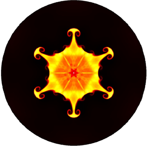
Shown in figure 7 is the evolution of the shock wave and gaseous interface depicted by density contours. It can be seen that the positions and patterns of both the shock and interface at six selected moments compare well with the experimental images. In figure 8 we displayvariations of the amplitude  $\eta (t)$ and corresponding growth rate
  $\textrm {d}\eta (t)/\textrm {d}t$, which can be divided into three stages. In stage I (from point
  $\textrm {A}$
  $(t=0\ \mathrm {\mu }\textrm {s}$) to
  $\textrm {B}$
  $(t=6.9\ \mathrm {\mu }\textrm {s}$)), the IS compresses and accelerates the interface. The post-shock amplitude is usually estimated by
  $\eta _B=(2\eta _A-V_{INF} T)/2$, where
  $T=2\eta _A/V_{IS}$ denotes the time for the IS to travel from the interfacial crest to trough with constant speed
  $V_{IS}$. This leads to a compression rate
  $\eta _B/\eta _A=1-V_{INF}/V_{IS}$ (Meshkov Reference Meshkov1969; Ding et al. Reference Ding, Si, Yang, Lu, Zhai and Luo2017). However, the calculated value 0.77 is evidently larger than the measured value
  $0.66$ from figure 7. Here, the IS is assumed to pass through the first and second halves of the interface at
  $V_{IS}$ and
  $V_{TS}$, respectively, which gives rise to
  $T=\eta _A/V_{IS}+\eta _A/V_{TS}$ and a modified compression rate
 \begin{equation} \frac{\eta_B}{\eta_A}=1-\frac{V_{INF}}{2} \left(\frac{1}{V_{IS}}+\frac{1}{V_{TS}}\right). \end{equation}
The resultant compression rate of 0.656 coincides with the measurement. In stage II (from point  $\textrm {B}$
  $(t=6.9\ \mathrm {\mu }\textrm {s}$) to
  $\textrm {D}$
  $(t=145\ \mathrm {\mu }\textrm {s}$)), the perturbations first grow with increasing growth rate due to the RM instability and BP effects. After the TS is reflected from the centre, the inward moving interface slows down gradually and induces the RT stabilizing effect that suppresses the growth of the perturbations (Ding et al. Reference Ding, Si, Yang, Lu, Zhai and Luo2017; Luo et al. Reference Luo, Zhang, Ding, Si, Yang, Zhai and Wen2018). Consequently, the growth rate decreases even down to negative values and the curve for the amplitude tends to bend down. Here, point D denotes the reshock time, while points C and E correspond roughly to the moments the RTS hits the bubble and spike of the diffusive interface, respectively. In stage III (after point D), the perturbations undergo shock compression again and a phase reversal is observed simultaneously (not shown here) (Brouillette Reference Brouillette2002). The amplitude curve drops slightly and then rises dramatically with much stronger amplification than the first impingement. After reshock, the material interface experiences a deceleration motion away from the centre, in which the RT instability effect tends to intensify the perturbations, while the BP effect is inclined to suppress the growth of the perturbation amplitude.

Figure 7. Evolution of density contours for the single-mode cylindrical RM instability: comparison between the present simulation (bottom halves) and experiment (top halves) (Lei Reference Lei2017).

Figure 8. Evolutions of the amplitude  $\eta (t)$ (red solid line) and corresponding growth rate
  $\textrm {d}\eta (t)/\textrm {d}t$ (blue dot-dashed line) for the single-mode cylindrical RM instability in comparison with the experimental data (black squares) (Lei Reference Lei2017).
Bell (Reference Bell1951) extended the linear model for the perturbation growth rate of the planar RT instability (Taylor Reference Taylor1950) into a cylindrical geometry, aiming to model the corresponding perturbation growth in the early stage. Under a small-perturbation assumption, the simplified compressible model takes the form
 \begin{align} \dot{\eta}(t)&=\frac{R_0^2}{R^2(t)}\dot{\eta}_0+\frac{nA-1}{R^2(t)}\int_{t_0}^{t}R(\tau)\ddot{R}(\tau)\eta(\tau)\,\textrm{d}\tau \nonumber\\ & \quad +\frac{c}{R^2(t)}\left[ \int_{t_0}^{t}R(\tau)\dot{R}(\tau)\eta(\tau)\,\textrm{d}\tau+\int_{t_0}^{t}R^2(\tau)\dot{\eta}(\tau)\,\textrm{d}\tau \right], \end{align}
where the single and double dots denote the first and second derivatives with respect to time  $t$,
$t$,  $R(t)$ is the averaged trajectory of the interface and
  $A=(\rho _2-\rho _1)/(\rho _2+\rho _1)$ is the post-shock Atwood number with
  $\rho _1$ and
  $\rho _2$ representing the inner and ambient fluid densities, respectively. We denote by
  $R_0$ and
  $\dot {\eta _0}$ the position and amplitude at
  $t=t_0$, respectively. The first two terms on the right-hand side of (3.2) appear as an incompressible model, which cannot correctly describe the evolution of the perturbations in stage II due to ignorance of the compressibility effect, as argued by Ding et al. (Reference Ding, Si, Yang, Lu, Zhai and Luo2017). Although a decay factor
  $Z$ is proposed for the incompressible model to compensate for the loss of the compressibility effect, the free factor
  $Z$ is determined a posteriori and varies from case to case, which reduces the reliability of this model.
The parameter  $c=-\dot {\rho _1}/\rho _1=-\dot {\rho _2}/\rho _2$ characterizes the compression rate of the species, which is considered as a constant and approximated by
  $c=\dot {V_1}/{V_1}\approx [1-(R_{min}/R_0)^2]/{t_{res}}$ (Lei Reference Lei2017). Here
  $V_1$ denotes the volume of the inner fluid,
  $R_{min}$ is the smallest radius of the interface during propagation and
  $t_{res}$ denotes the time when the reshock happens. In the present simulation,
  $A\approx -0.65$ and
  $c\approx 0.0057\ \mathrm {\mu }\textrm {s}^{-1}$. It should be mentioned that direct use of the measured amplitude
  $\eta (t)$ in (3.2) may lead to an unsatisfactory result in that the interface has a premixed width, while this compressible model is only suitable for a sharp interface. As shown in figure 9, with measured initial post-shock amplitude
  $\eta (0)^{+}=0.53\ \textrm {mm}$ and growth rate
  $\dot {\eta }(0)^{+}=5.4\ \textrm {m} \ \textrm {s}^{-1}$, the curve of the predicted total amplitude by Bell's compressible model (solid brown line) deviates from the simulation and experimental results in late stage II. Again, it is assumed that the premixed width
  $\eta _{up}$ of the interface and the exact amplitude of the perturbations
  $\eta _{sm}$ decouple from each other and evolve individually with time. The premixed width
  $\eta _{up}(t)$ can be obtained directly from the simulation of the unperturbed interface, and
  $\eta _{sm}(t)$ can be determined by (3.2) provided that proper initial amplitude and growth rate are specified. The first and second terms on the right-hand side of (3.2) represent the contributions of the RM instability (
 $\eta _{RM}$) and RT stability/instability (
 $\eta _{RT}$), respectively, while the third term can be regarded as the compressibility effect (
 $\eta _{C}$). The BP effect is coupled into each term and difficult to isolate from others. Thus, the total measured amplitude
  $\eta (t)$ can be decomposed as
 \begin{equation} \eta=\eta_{up}+\eta_{sm}=\eta_{up}+\eta_{RM}+\eta_{RT}+\eta_{C}. \end{equation}
Figure 9. Total amplitude  $\eta (t)$ (blue solid line with circles) and all contribution terms calculated by the modified compressible model. The data from Bell's original model (brown solid line) and the present simulation (red solid line) and experiment (black squares) (Lei Reference Lei2017) are added for comparison.
To use the compressible model ((3.2) and (3.3)),  $R(t)$ should be specified as the trajectory of the unperturbed interface with the same premixed width as the initially perturbed case. Point B is chosen as the starting time
  $t_0$ to obtain the post-shock amplitude
  $\eta _{sm}(0)^{+}=0.21\ \textrm {mm}$ and growth rate
  $\dot {\eta }_{sm}(0)^{+}=4.4\ \textrm {m}\,\textrm {s}^{-1}$ from the simulations. A numerical integration of (3.2) yields the modelled amplitude
  $\eta _{sm}(t)$. In figure 9 we show
  $\eta _{sm}(t)$ together with its composing terms, as well as the evolution of
  $\eta _{up}(t)$. It is clearly seen that the modified compressible model shows very good agreement with the present simulation in stage II before reshock. At the beginning, the effect of the RM instability is dominant and triggers the growth of disturbances. The coupled RT stabilizing and BP effect firstly keeps positive, and then starts to suppress the perturbation growth due to deceleration of the interface. The coupled compressibility and BP effect always plays a positive role, indicating that the compressibility effect yields to the BP effect and is not significant for the present incident shock strength.
3.3. Further validation of the refined Bell model
Eight supplementary test cases are considered to further validate the modified compressible model. In test cases 1–5, the premixed interfacial width is set identically to  $\eta _{up}=0.50\ \textrm {mm}$, while different amplitudes of initial single-mode perturbations are specified as listed in table 2. The species are pure SF
 $_6$ surrounded by pure air with the properties listed in table 1. Note that case 1 is designed as the ‘base-line’ case without initial perturbations. The modified model can reproduce all the simulated results (cases 2–5) with satisfactory accuracy, as shown in figure 10. Moreover, we find that, as the initial amplitude increases, the accuracy of the modified model tends to decrease due to the violation of the small-perturbation assumption. In other words, with an evolution of the unperturbed interface, the modified compressible model can successfully predict the growth history of perturbations before reshock for any single-mode perturbed interface, as long as they are under the same conditions and the small-perturbation assumption approximately applies.
Table 2. The measured initial amplitude ( $\eta (0)$), premixed width (
 $\eta _{up}(0)$) and exact single-mode amplitude (
 $\eta _{sm}(0)$) for eight test cases. Here
  $\eta _{sm}(0)^{+}$ and
  $\dot {\eta }_{sm}(0)^{+}$ denote the exact post-shock amplitude and growth rate, respectively.


Figure 10. Total amplitude  $\eta (t)$ obtained from the modified compressible model for test cases 2–5 in table 2 with the same premixed width but different initial single-mode amplitudes, in comparison with corresponding simulation results. The black solid line is obtained from a DNS of the initially unperturbed case (test case 1).
In test case 6, the initial single-mode amplitude is set to  $\eta _{sm}(0)=2.00\ \textrm {mm}$ with the premixed width unchanged to evaluate the validity of the improved model in predicting the growth rate of high-amplitude perturbations. The temporal evolution of the total amplitude
  $\eta (t)$ given by the improved model (orange squares) is compared with that calculated using a DNS (orange solid line) in figure 11. The corresponding result for the evolution of the unperturbed interface is plotted as the orange dot-dashed line. As can be seen, the new model first overestimates the interface amplitude and then underestimates it during the deceleration period just before the reshock event. The model cannot produce the plateau observed in a DNS, which is attributed to the compromise of the RM instability effect in competition with the RT stabilizing effect discussed previously. The failure of the improved model in this ‘large-initial amplitude case’ results from the violation of the small-perturbation assumption of Bell's model. Shown in figure 12 are density contours at six time points for the single-mode cylindrical RM instability for test case 6, which depict the temporal evolution of shock waves and the gaseous interface. At
  $t=114\ \mathrm {\mu }\textrm {s}$, the modelled total perturbation amplitude
  $\eta (t)$ reaches its maximum and shows the maximum error in comparison with the DNS data. In fact, the ratio of the perturbation amplitude
  $\eta (t)$ to the wavelength
  $\lambda (t)=2{\rm \pi} {}R(t)/n$ is
  ${\sim}0.425$, which indicates that the growth of the interfacial perturbations has already entered a nonlinear stage. After this time point, the bubble structures immediately undergo the impingement of the RTS, which results in more complex flow mixing, such as phase reversal of the material interface (see the picture at
  $t=142\ \mathrm {\mu }\textrm {s}$). This explains why the improved model does not apply to the prediction of the growth of large initial perturbations, especially when the RTS approaches the interface for a second time.

Figure 11. Total amplitude  $\eta (t)$ obtained from the modified compressible model for test cases 6 (large initial single-mode amplitude) and 8 (large premixed width) in table 2, in comparison with the corresponding DNS results. The orange and green dot-dashed lines are obtained from DNS of the initially unperturbed cases (test cases 1 and 7, respectively).

Figure 12. Evolution of density contours for the single-mode cylindrical RM instability: test case 6 (large initial single-mode amplitude) in table 2.
In test case 8, the premixed width is set identically to  $\eta _{up}=1.50\ \textrm {mm}$, while the initial single-mode amplitude is set to
  $\eta _{sm}(0)=0.25\ \textrm {mm}$ in order to verify the effectiveness of the revised model for a much more diffuse initial interface. The temporal evolution of the total amplitude
  $\eta (t)$ reproduced by the improved model (green circles) is also depicted in figure 11 in comparison with that extracted from a DNS (green solid line). Note that the corresponding evolution of the unperturbed interface is displayed as the green dot-dashed line. It is clearly seen that the modelled result almost collapses onto the DNS data, which implies that the improved Bell model still holds for the amplitude evolution with a very diffuse interface as long as the initial perturbations satisfy the small-perturbation hypothesis.
We note from (3.2) that the start time  $t_0$ of the integration can be selected arbitrarily during the development of the RM instability. Therefore, we conjecture that the improved Bell model can be applied to the prediction of the amplitude evolution before and after reshock using a piecewise-integrator algorithm provided that the local amplitude of the interface does not violate the small-perturbation assumption. To this end, test case 3 in table 2 is evaluated up to the nonlinear stage after reshock without loss of generality. Shown in figure 13 is the evolution of the total amplitude
  $\eta (t)$ obtained from the modified Bell model before reshock (green triangles) and after reshock (orange triangles) for test case 3, in comparison with the corresponding DNS result (red solid line). As can be seen, the accuracy of the proposed model is acceptable after reshock up to
  $t\approx 235\ \mathrm {\mu }\textrm {s}$. After that, the improved Bell model apparently overestimates the growth rate of the perturbation amplitude given by a DNS. It ought to be mentioned here that the RT and compressibility effects (coupled with the BP effect) play opposite roles in the development of material mixing after reshock as compared with those before reshock. After the RTS passes through the interface for a second time, the interface experiences a deceleration motion and, consequently, the RT instability effect reinforces the growth of the interfacial perturbations. In contrast, the compressibility effect coupled with the BP effect of the diverging motion tends to suppress the amplification of the perturbations. Although the improved model can successfully reflect these physical procedures, it fails to produce the accurate perturbation amplitude during the nonlinear stage due to the violation of the small-perturbation assumption of Bell's model. The appearance of nonlinearity can be clearly seen from the evolution of the interfacial structures. Depicted in figure 14 are density contours extracted from test case 3 at three typical time points, i.e. just before reshock (
 $t=135\ \mathrm {\mu }\textrm {s}$), immediately after completion of phase reversal (
 $t=186\ \mathrm {\mu }\textrm {s}$) and immediately after the formation of mushroom structures on spikes (
 $t=273\ \mathrm {\mu }\textrm {s}$). The post-reshock picture indicates that strong nonlinearity appears between
  $t=235\ \mathrm {\mu }\textrm {s}$ and
  $t=273\ \mathrm {\mu }\textrm {s}$ when the improved Bell model becomes invalid. In fact, the modelled amplitude strongly deviates from the DNS data when the secondary instability structures appear on the stems of spikes, as observed in figure 14 at
  $t=273\ \mathrm {\mu }\textrm {s}$.

Figure 13. Total amplitude  $\eta (t)$ obtained from the modified compressible model before reshock (green triangles) and after reshock (orange triangles) for test case 3 in table 2, in comparison with the corresponding DNS result (red solid line). The blue dot-dashed line is obtained from DNS of the initially unperturbed case (test case 1).

Figure 14. Evolution of density contours for the single-mode cylindrical RM instability before and after reshock for test case 3 in table 2.
4. Conclusions
In summary, we study the 2-D single-mode RM instability in a cylindrical geometry using the DNS method. Focus is placed on the perturbation growth history in the early stage. The evolution of interfacial disturbances is compared with the cylindrical shock tube experiment (Lei et al. Reference Lei, Ding, Si, Zhai and Luo2017), and both qualitative and quantitative consistencies are observed before reshock provided that the premixed width is taken into account. The amplitude and growth rate curves are obtained and divided into three stages. In the early stage, the perturbation amplitude undergoes a decrease due to shock compression. In the middle stage (before reshock), the RM instability and BP effects are dominant first and contribute to the perturbation growth, and then the perturbations are significantly suppressed by the dominant RT stabilizing effect. In the late stage (after reshock), the perturbations experience a dramatic amplification process due to more complicated waves. The evolution and underlying physics of the present cylindrical RM instability are well addressed by a refined compressible Bell model, which is composed of an unperturbed part, an RM instability part, an RT stabilization part and a compressibility part. Given the development history of an unperturbed interface, the early-stage evolution of the single-mode cylindrical RM instability of the same family (with the same premixed width) can be reproduced accurately by the improved model as long as the initial perturbation amplitude satisfies the small-perturbation assumption or the ratio of the initial perturbation amplitude to wavelength is less than 5 %. Furthermore, the refined Bell model can also be applied to prediction of the growth rate of the perturbation amplitude in the post-reshock stage before the appearance of strong nonlinearity by using a piecewise-integrator method. The present work may help enrich understanding and modelling of the convergent RM instability, especially for the case driven by much stronger incident shock wave. The extension of the present model to a strongly nonlinear-stage RM instability is open for further research.
Acknowledgements
We are grateful to Y. Liang for many fruitful discussions on this work. Numerical simulations were performed on Tianhe-2 at the National Supercomputer Center in Guangzhou, China. We acknowledge financial support from the National Natural Science Foundation of China (grants no. 91852112 and no. 11988102). This work was also supported by the Challenge Program (grant no. JCKY2016212A501).
Declaration of interests
The authors report no conflict of interest.


