


1. Introduction
Hypersonic vehicles, such as space planes and space capsules, re-entering Earth or entering the atmosphere of distant planets, sustain prolonged thermal loads on both external and internal surfaces. When models of such vehicles are tested in a ground-based facility, for example, a wind tunnel or a shock tunnel, the model surface is generally ‘cold’, that is, the surface temperature is a very small fraction of the reservoir or recovery temperature. Theoretical works on boundary layers and viscous effects, however, more often than not assume an adiabatic wall. It is only recently that wall or surface temperature effects (hence heat flux), which significantly influence hypersonic flows, have received adequate attention.
Wall temperature effects are thus a significant issue in the design of experiments dealing with high-enthalpy hypersonic flows. Depending on the type of facility, the wall temperature of the experimental model can be considerably different from that of a hypersonic vehicle in actual flight. Such a drawback is common in experiments carried out in high-enthalpy impulse facilities, for example, shock or gun tunnels. In such facilities, the test times are short, typically a few milliseconds, so that the surface temperature of the model has insufficient time to reach the adiabatic or recovery temperature. The model temperature, under these conditions, remains close to the room or ambient temperature and so is not an accurate reflection of high-temperature effects on the surface that exist in flight. These effects, such as boundary layer transition, flow separation, surface catalycity, and chemical and thermal non-equilibrium, can have severe consequences on the controllability and stability of the vehicle. A well-known example is the Space Shuttle pitch anomaly, where real gas and viscous effects required the flap deflection to be increased to  $16^{\circ }$ instead of the predicted
  $7^{\circ }$ because those predictions were based on ‘cold’ tunnel data (Brauckmann, Paulson & Weilmuenster Reference Brauckmann, Paulson and Weilmuenster1995). This is an example to illustrate the importance of replicating, as much as possible, flight conditions in ground-based facilities.
One of the early important papers to consider wall temperature effects on shock-induced separation was by Gadd (Reference Gadd1957a,Reference Gaddb). Gadd showed that for a laminar boundary layer, the separation pressure is unaffected by wall heating or cooling. His second observation was that pressure gradients are sharper with wall cooling and slowly varying with wall heating. The length of the interaction region was shown to vary as  $T_w^{-3/2}$. Nielsen, Lynes & Goodwin (Reference Nielsen, Lynes and Goodwin1966) confirmed the independence of the separation pressure with respect to the wall temperature, but the interaction extent varied with wall temperature with an index
  $n \approx 1.3$. The temperature range examined by Nielsen et al. (Reference Nielsen, Lynes and Goodwin1966) was much greater than that by Gadd (Reference Gadd1957a,Reference Gaddb). Both the Gadd (Reference Gadd1957a,Reference Gaddb) and Nielsen et al. (Reference Nielsen, Lynes and Goodwin1966) studies were restricted to supersonic Mach numbers.
Recently, there has been a renewed interest in the wall temperature effects arising out of hypersonic research. Marini (Reference Marini2001) investigated the wall temperature effects on a shock/boundary layer interaction (SBLI) and the separation induced by a compression ramp in laminar hypersonic flow with a sharp leading-edge. The investigation included both numerical simulations as well as experimental data from various sources. The Mach and Reynolds number ranges were 6–14 and  $2.36\times 10^5 - 4 \times 10^6$ per metre, respectively. The wall to stagnation temperature ratio (
 $T_w / T_0$) ranged between
  $0.17$ and
  $0.46$. Both two-dimensional and axisymmetric hollow cylinder flare geometries were studied. The corner/flare angles of
  $10^{\circ }$ and
  $15^{\circ }$ were considered. The results, in general, showed that heating the wall increased the susceptibility to separation as a result of the increased boundary layer thickness as well as the less full profile, and once separated, heating increased the separation length. Cooling had the opposite effect. Separation was largest with an adiabatic wall, as expected. The investigation highlighted the importance of heating the experimental models in wind tunnel facilities and not placing undue reliance on cold tunnel data. The two-dimensional finite-span effects were seen to be quite significant in the presence of separation and, once separation occurred, the separation size reduced towards the spanwise direction. Overall, both peak pressure and heating reduced with finite-span. With the hollow cylinder flare model, the flow remained two-dimensional when transverse curvature effects were small over the cylinder up to separation but post separation and towards reattachment, the flow no longer remained two-dimensional with cross-flows resulting in higher plateau pressures but lower peak pressure and lower peak heat flux.
Another notable contribution on wall temperature effects in a laminar hypersonic SBLI with separation is the experimental investigation by Bleilebens & Olivier (Reference Bleilebens and Olivier2006), who pre-heated a compression corner model of finite-span to obtain varying wall to stagnation temperature ratios from  $0.193$ to
  $0.553$. The corner angle was
  $15^{\circ }$. The unit Reynolds number range was approximately one to nearly nine million. The nominal Mach number was
  $8$. The main conclusions were that the separation size increased with an increase in the wall temperature ratio. Another observation was that transition took place in the separated shear layer before reattachment but this did not affect the size of the separation bubble. The experimental data showed that separation bubble scaling could be achieved reasonably well by modifying the adiabatic wall correlation of Katzer (Reference Katzer1989). Another correlation based on Katzer (Reference Katzer1989) has recently been used by Chang et al. (Reference Chang, Chan, McIntyre and Veeraragavan2021) for an impinging shock SBLI on a heated flat plate in a Mach 7 high-enthalpy hypersonic flow. They found that the correlation of Bleilebens & Olivier (Reference Bleilebens and Olivier2006) for a heated compression ramp at hypersonic Mach numbers was not quite applicable to an impinging shock SBLI. This was attributed to higher shock strengths in their experiments.
In the same vein as Bleilebens & Olivier (Reference Bleilebens and Olivier2006), Wagner et al. (Reference Wagner, Schramm, Hannemann, Whitside and Hickey2017) conducted an experimental investigation using a two-dimensional finite-span compression ramp model by pre-heating only the upstream flat plate and not the ramp surface. A small gap was left at the hinge line and it was assumed that the unheated ramp surface did not affect the interaction process. The main purpose of the experiment was to study the state of the boundary layer before interaction by changing the leading-edge bluntness from sharp to  $200\ \mathrm {\mu }\textrm {m}$ thickness. The wall to stagnation temperature ratio varied from
  $0.1$ to
  $0.3$. The Mach and unit Reynolds numbers were
  $7.4$ and
  $6.65\times 10^6$ per metre, respectively. The ramp angles were
  $15^{\circ }$ and
  $30^{\circ }$. It was shown that both a sharp leading-edge and increasing the wall temperature had a destabilising effect on the boundary layer prior to interaction, while blunting the leading-edge had a stabilising effect. There were several deficiencies in their investigation that were not addressed, mainly finite-span effects, which were highlighted by discrepancies between their two-dimensional numerical simulations and experimental data, and the assumption that the unheated ramp surface had no effect on the interaction process.
There have been several theoretical/numerical studies on wall temperature effects on SBLI-induced separation. These started with Brown, Cheng & Lee (Reference Brown, Cheng and Lee1990) and then followed by Kerimbekov, Ruban & Walker (Reference Kerimbekov, Ruban and Walker1994), Cassel, Ruban & Walker (Reference Cassel, Ruban and Walker1996), Shvedchenko (Reference Shvedchenko2009), Neiland, Sokolov & Shvedchenko (Reference Neiland, Sokolov and Shvedchenko2009) and Egorov, Neiland & Shredchenko (Reference Egorov, Neiland and Shredchenko2011). Brown et al. (Reference Brown, Cheng and Lee1990) modified the triple-deck-based interaction equation to take into account wall temperature effects. They also classified wall temperature effects into subcritical ( $T_w / T_0 \ll T_w^* / T_0$), transcritical (
 $T_w / T_0 = O (T_w^* / T_0)$) and supercritical (
 $T_w / T_0 \gg T_w^* / T_0$). Here
  $T^*_w / T_0$ is a critical wall temperature ratio which is purely a function of hypersonic viscous interaction, the specific heat ratio
  $\gamma$ and properties of the upstream boundary layer. The authors solved the modified interaction equation numerically and showed that cooling has a strong effect in drastically reducing upstream influence and in reducing the extent of separation. The triple-deck-based Brown et al. (Reference Brown, Cheng and Lee1990) approach was followed by Kerimbekov et al. (Reference Kerimbekov, Ruban and Walker1994), who analysed the effects of strong wall cooling, wherein the interaction was shown to be mainly between the main deck and the outer deck (inviscid/inviscid). The wall cooling effect was classified in terms of the Neiland number
  $N$, wherein
  $N \gg 1$ defines strong cooling (supercritical),
  $N = O (1)$ moderate cooling (transcritical) and
  $N \ll 1$ indicates very little cooling (subcritical). A subsequent paper by Cassel et al. (Reference Cassel, Ruban and Walker1996) followed a similar approach as Kerimbekov et al. (Reference Kerimbekov, Ruban and Walker1994) and showed that strong cooling (
 $N \gg 1$) has a stabilising effect and subcritical cooling (
 $N \ll 1$) has a destabilising influence on the boundary layer. Their conclusion that separation can be completely eliminated by strong wall cooling is, however, shown to be contrary to earlier evidence (Nielsen et al. Reference Nielsen, Lynes and Goodwin1966) as well as the later observations of Brown et al. (Reference Brown, Cheng and Lee1990). While in the paper by Cassel et al. (Reference Cassel, Ruban and Walker1996) it is stated that ‘sufficient level of wall cooling eliminates separation altogether’, Brown et al. (Reference Brown, Khorrami, Neish and Smith1991) state (p. 336 of their paper) ‘contrary to common belief, examination of available numerical results indicate that separation cannot be prevented or delayed effectively by merely lowering the wall temperature but the thickness and the length scale of the lower deck and hence upstream influence are drastically reduced.’ The evidence from Nielsen et al. (Reference Nielsen, Lynes and Goodwin1966) shows that even at
  $T_{w} / T_{ad} < 0.133$, separation is not completely eliminated though the interaction length goes nearly to zero. Mention may also be made here of the work by Seddougui, Bowles & Smith (Reference Seddougui, Bowles and Smith1991), who specifically discussed the effects of wall cooling but with emphasis on stability and transition. They concluded that moderate cooling has a destabilising effect on a compressible boundary layer.
Recently, some Navier–Stokes based numerical simulations of large-scale separated flows with wall temperature effects have been published: Neiland et al. (Reference Neiland, Sokolov and Shvedchenko2009); Shvedchenko (Reference Shvedchenko2009); Egorov et al. (Reference Egorov, Neiland and Shredchenko2011); and Khraibut et al. (Reference Khraibut, Gai, Brown and Neely2017). These studies consider not only effects of wall temperature on primary separation but also the development of secondary separation. A similarity parameter, also called a scaled angle, based on the geometric ramp angle  $\alpha ^*$, is defined as (Stewartson Reference Stewartson1970)
 \begin{equation} \alpha = \frac{ \alpha^*}{C^{1/4} \lambda^{1/2} } \left( \frac{Re}{M^2 - 1} \right)^{1/4}, \end{equation}
which includes the effect of viscosity through Chapman–Rubesin constant  $C$, wall-shear constant
  $\lambda$, along with Mach and Reynolds numbers. This parameter is based on triple-deck scales, as explained by Stewartson (Reference Stewartson1975) and Rizzetta, Burggraf & Jenson (Reference Rizzetta, Burggraf and Jenson1978) as well as by Korolev, Gajjar & Ruban (Reference Korolev, Gajjar and Ruban2002). Some authors have used slightly different versions of this parameter, for example, Shvedchenko (Reference Shvedchenko2009) and Neiland et al. (Reference Neiland, Sokolov and Shvedchenko2009) define the scaled angle as
  $\alpha ^* Re^{1/4}$, while Egorov et al. (Reference Egorov, Neiland and Shredchenko2011) define the scaled angle as
  $\alpha ^* (Re / (M^2 - 1))^{1/4}$. In this paper, we have used the Stewartson–Rizzetta definition for consistency. In general, it is found that separation size and occurrence of secondary separation is dependent on the value of the scaled angle and the wall temperature ratio. With the increase in both, separation size increases and further increase in both eventually promotes secondary separation, and with still further increase, fragmentation of secondary separation into multiple vortices. Shvedchenko (Reference Shvedchenko2009), Egorov et al. (Reference Egorov, Neiland and Shredchenko2011) and Khraibut et al. (Reference Khraibut, Gai, Brown and Neely2017) delineate the various separation stages when the above flow features develop. In terms of the present definition of the scaled angle, steady primary separation appears at
  $\alpha \leq 2$ and secondary separation develops at
  $3 \leq \alpha \leq 4$ (Gai & Khraibut Reference Gai and Khraibut2019). Suffice to say that primary separation occurs at a lower value of the scaled angle with a hotter wall while secondary separation occurs at a higher scaled angle when the wall is hotter. Results from Egorov et al. (Reference Egorov, Neiland and Shredchenko2011) also show that in the case of primary separation, the scaled angle changes very little with changes in Mach number for an adiabatic wall while it increases with Mach number for a cold wall. The difference in the value of the scaled angle also increases with the increase in Mach number. In the case of secondary separation with the adiabatic wall, there is a slight decrease in the scaled angle with the increase in Mach number. With the cold wall, the same trend is seen but the rate of decrease is even smaller.
Effects of small bluntness on shock-induced separation at hypersonic Mach numbers has been investigated extensively in the past and in recent years. The bluntness effect is critical from a practical point of view because in the fabrication of experimental models, for example, the leading-edge sharpness is restricted by manufacturing limitations. Earlier studies of bluntness effects were largely related to transition in boundary layers from laminar to turbulent (Moeckel Reference Moeckel1957; Nagamatsu, Sheer & Wisler Reference Nagamatsu, Sheer and Wisler1966; Softley Reference Softley1969; Stetson Reference Stetson1979). Studies related to bluntness effects on pressure, skin-friction and heat transfer in both attached and separated flows have also been conducted, for example, Bertram (Reference Bertram1954), Bertram & Henderson (Reference Bertram and Henderson1958), Cheng et al. (Reference Cheng, Hall, Golian and Hertzberg1961), Holden (Reference Holden1971), Stollery (Reference Stollery1972), and in recent years, Mason & Lee (Reference Mason and Lee1994), Smith & Khorrami (Reference Smith and Khorrami1994), Mallinson, Gai & Mudford (Reference Mallinson, Gai and Mudford1996), Marini (Reference Marini1998), Borovoy, Skuratov & Struminskaya (Reference Borovoy, Skuratov and Struminskaya2008), Borovoy et al. (Reference Borovoy, Mosharov, Radchenko, Skuratov and Struminskaya2014), John & Kulkarni (Reference John and Kulkarni2014), Khraibut, Gai & Neely (Reference Khraibut, Gai and Neely2019) and Mallinson, Mudford & Gai (Reference Mallinson, Mudford and Gai2020).
An important breakthrough in the analysis of bluntness effects was the introduction of a similitude parameter  $\beta$, by Cheng et al. (Reference Cheng, Hall, Golian and Hertzberg1961), which combined the effects of both viscous interaction and bluntness in hypersonic flow. Thus
  $\beta = \bar {\chi }_\varepsilon / \kappa ^{2/3}$, where
  $\bar {\chi }_\varepsilon$ is the modified viscous interaction parameter, which takes into account viscous effects, and
  $\kappa$ is a parameter describing the bluntness effect. While Cheng et al. (Reference Cheng, Hall, Golian and Hertzberg1961) used this parameter to analyse bluntness and boundary layer displacement effects on flat plates at zero and non-zero incidence, Holden (Reference Holden1971) successfully used this parameter to delineate the flow separation on flat plate/ramp geometry. Later, Mallinson et al. (Reference Mallinson, Gai and Mudford1996) and Khraibut et al. (Reference Khraibut, Gai and Neely2019) analysed bluntness effects using this same parameter. Khraibut et al. (Reference Khraibut, Gai and Neely2019), in particular, showed that for ‘small’ bluntness (as defined later), the results were opposite to those found by Holden (Reference Holden1971). In another recent paper, Chuvakhov et al. (Reference Chuvakhov, Borovoy, Egorov, Radchenko, Olivier and Roghelia2017) studied the effects of small bluntness on separation in a two-dimensional finite-span compression corner flow and found that when the bluntness to flat plate length ratio (
 $t/L$) is less than approximately
  $0.015$, the separation length increases with increase in bluntness, which is in agreement with the findings of Khraibut et al. (Reference Khraibut, Gai and Neely2019). This is also in agreement with the theoretical analysis by Lagrée (Reference Lagrée1991).
In the following, § 2 presents a brief description of the theoretical aspects, in particular, the triple-deck approach, where it is shown how wall temperature and bluntness effects can be included in the interaction equation. Section 3 describes the flow configuration. Section 4 deals with the numerical methodology in which both N–S simulations, using the solver US3D, and the triple-deck equations using the algorithm of Cassel, Ruban & Walker (Reference Cassel, Ruban and Walker1995), based on the method of Ruban (Reference Ruban1978), are discussed. Section 5 presents various results for both N–S simulations and triple-deck solutions (§§ 5.1 and 5.2) and § 6 discusses these results in detail. Finally, conclusions are drawn in § 7.
2. Theoretical considerations
2.1. Asymptotic structure of a supersonic boundary layer over an adiabatic wall
Figure 1 shows the structure of a supersonic boundary layer over an adiabatic wall as outlined by the triple-deck theory. The dimensional coordinates  $x^*$ and
  $y^*$ are normalised by the length
  $L$ of the flat plate from the leading-edge to the corner so that
  $x = O(1)$ and
  $y=O(\varepsilon ^4)$ in the usual boundary layer structure described by the Blasius equation, where
  $\varepsilon = Re^{-{1}/{8}}$ is the scaling parameter in the triple-deck theory, and
  $Re$ is the Reynolds number based on the flat plate length and free stream conditions and is assumed to be infinitely large. The boundary layer is disturbed by a small pressure perturbation of the order of
  $O(\varepsilon ^2)$, which is independent of the agent producing the disturbance by virtue of the ‘free-interaction’ concept (Chapman, Kuehn & Larson Reference Chapman, Kuehn and Larson1958; Neiland Reference Neiland1969; Stewartson & Williams Reference Stewartson and Williams1969). The reaction of the boundary layer to this pressure disturbance is such that it can be divided into three regions or ‘decks’, where the flow is governed by different governing equations. The main deck, where the flow is inviscid and rotational, has a wall-normal extension of the order of
  $O(\varepsilon ^4)$. The lower deck, where the flow is viscous and incompressible, is of the order of
  $O(\varepsilon ^5)$. The upper deck is of the order of
  $O(\varepsilon ^3)$ and can be described by Ackeret or Prandtl–Glauert equations.

Figure 1. Asymptotic structure of a boundary layer approaching the corner according to the triple-deck theory.
The asymptotic structure, as described above, was first devised independently by Stewartson & Williams (Reference Stewartson and Williams1969) and Neiland (Reference Neiland1969). The analysis reduces the number of equations required to model the interaction between the boundary layer and the pressure perturbation. The relevant equations are the incompressible flow equations of the lower deck
 $$\begin{gather} \frac{\partial u}{\partial x} + \frac{\partial v}{\partial y} = 0, \end{gather}$$
 $$\begin{gather}\frac{\partial u}{\partial t} + u \frac{\partial u}{\partial x} + v \frac{\partial u}{\partial y} ={-} \frac{\partial p}{\partial x} + \frac{\partial^2 u}{\partial y ^2}, \end{gather}$$
and the ‘interaction law’, which links the pressure change with the growth of the lower deck through the Ackeret formula
 \begin{equation} p ={-} \frac{\textrm{d}A}{\textrm{d}x} + \frac{\textrm{d}f }{\textrm{d}x} , \end{equation}
where  $A(x)$ represents the displacement thickness of the subsonic region and
  $f(x)$ describes the body shape. The system of equations is closed by the boundary conditions
 $$\begin{gather} u \rightarrow y + A, \quad \text{when}\ y \rightarrow \infty, \end{gather}$$
 $$\begin{gather}u = v = 0, \quad \text{when}\ y \rightarrow 0, \end{gather}$$
 $$\begin{gather}u \rightarrow y, \quad \text{when} \ x \rightarrow - \infty. \end{gather}$$
2.2. Wall temperature and bluntness effects
For the case of a hypersonic boundary layer over an adiabatic wall, the interaction law was obtained by Neiland (Reference Neiland1970) using the tangent-wedge approximation, an approach followed by Stewartson (Reference Stewartson1975), Gajjar & Smith (Reference Gajjar and Smith1983) and Smith & Khorrami (Reference Smith and Khorrami1991). Wall temperature effects were taken into account by Brown et al. (Reference Brown, Cheng and Lee1990) and Neiland (Reference Neiland1973) using different approaches, which generated two different lines of thought. It should be pointed out, however, that it has been shown that the approach of Neiland (Reference Neiland1973) applies to a more general set of flow conditions. In Brown et al. (Reference Brown, Cheng and Lee1990), (2.2) is modified as
 \begin{equation} \frac{1}{\sigma} p + \frac{\textrm{d}p}{\textrm{d}x} ={-} \frac{\textrm{d} A}{\textrm{d}x}, \end{equation}
where  $\sigma$ is given as
 \begin{equation} \sigma = \left( \frac{s_w^*}{s_w} \right)^{4 \omega + 2}, \end{equation}
where  $\omega$ is the viscosity–temperature index,
  $s_w$ is the wall to stagnation temperature ratio
  $s_w = T_w / T_0$ and
  $s_w^*$ is the critical wall temperature ratio, defined as
 \begin{equation} s_w^* \sim \frac{T_w^*}{T_0} \sim \left[ \lambda^5 \gamma^{-{1}/{2}} \left( \frac{\gamma-1}{2} \right)^{{-}2} \bar{\chi} \right]^{{1}/{(4 \omega + 2)}}, \end{equation}
where  $\lambda$ is the normalised wall shear of the undisturbed boundary layer,
  $\gamma$ is the specific heat ratio of air and
  $\bar {\chi }$ is the hypersonic viscous interaction parameter
  $\bar {\chi } = M^{3} \sqrt {C / Re_{L}}$. Assuming a Blasius boundary layer
  $\lambda = 0.332$,
  $\gamma = 1.4$ and
  $\omega =0.5$,
  $\sigma$ takes the form (Khraibut et al. Reference Khraibut, Gai, Brown and Neely2017)
 \begin{equation} \sigma \sim 0.085 \bar{\chi} s_w^{{-}4}, \end{equation}
which indicates that  $\sigma$ increases with decreasing wall temperature.
According to Brown et al. (Reference Brown, Cheng and Lee1990), the flow is termed subcritical when  $s_w^* / s_w \gg 1$, transcritical when
  $s_w^* / s_w \sim O(1)$ and supercritical when
  $s_w^* / s_w \ll 1$.
It should be noted that these expressions are valid for small values of  $\bar {\chi }$. The expression (2.7) shows that
  $\sigma$ increases with decreasing wall temperature for fixed
  $\bar {\chi }$. Correspondingly, the scaled angle decreases as
  $s_w^2$. It shows
  $\sigma$ to be in the subcritical to transcritical range. Indefinitely decreasing
  $s_w$ cannot completely eliminate separation but it does substantially reduce the upstream influence (Brown et al. Reference Brown, Cheng and Lee1990). This is in contrast to Nielsen et al. (Reference Nielsen, Lynes and Goodwin1966), who concluded that in cold wall supersonic flow, upstream influence could be eliminated when the wall-to-stagnation temperature ratio was less than approximately
  $0.115$.
Just as the wall temperature effect is an additional term to the simple interaction law ((2.2)), one can include the effect of bluntness into the interaction law. It has been suggested by Lagrée (Reference Lagrée1991) that the effect of ‘small’ bluntness can be described in terms of a small parameter  $\eta$, which is proportional to the leading-edge bluntness
  $t^*$ normalised by a characteristic length
  $L$ (such as the flat plate upstream of a compression corner) and inversely proportional to the upper-deck scale
  $\varepsilon ^3 L$. Lagrée (Reference Lagrée1991) assumes that the entropy layer formed by blunting the leading-edge is small, which he calls the ‘fourth’ deck. This is the region between the upper or the main deck and the outer inviscid region. Lagrée (Reference Lagrée1991) calls the combined entropy layer/boundary layer as one and the lower viscous layer as the second of the two-layer fluid. He then assumes that disturbances from the lower viscous layer are transmitted to the upper layer. This also implies that
  $\partial p / \partial y \approx 0$. He then proposes the interaction law
 \begin{equation} p + \eta \left( \frac{ \textrm{d} p }{ {\textrm{d}x} } \right) ={-} \frac{\textrm{d} A}{\textrm{d}x}, \end{equation}
where  $\eta \ll 1$ and the second term of the left-hand side takes into account the effect of blunting. See the paper by Lagrée (Reference Lagrée1991) for details.
Thus for highly cooled walls (subcritical), the main deck contribution dominates over the lower viscous layer with the interaction between the outer entropy layer (the fourth deck) and the main deck of the boundary layer also dominating over the lower viscous layer. The combined effect of these two phenomena of cooling and bluntness on flow separation will be described in § 6.4.
3. Flow condition and model configurations
The flow condition, named Condition E herein, has been extensively used previously (Park, Gai & Neely Reference Park, Gai and Neely2010; Khraibut et al. Reference Khraibut, Gai, Brown and Neely2017; Prakash et al. Reference Prakash, Le Page, McQuellin, Gai and O'Byrne2019). The details are given in table 1. The wall temperatures chosen for this study are  $T_w= 300, 450, 600, 750, 900, 1050\ \textrm {K}$, which give wall-to-stagnation temperature ratios
  $s_w = T_w / T_0 = 0.095, 0.143, 0.191, 0.238, 0.286, 0.333$. The critical wall temperature ratio is
  $T_w^* / T_0 = 0.7$, so the boundary layer is subcritical for all cases according to the criteria of Brown et al. (Reference Brown, Cheng and Lee1990) and Cheng (Reference Cheng1993).
Table 1. Free stream conditions (Park et al. Reference Park, Gai and Neely2010).

The dimensions of the finite-span compression corner, named ‘finite-span model’ (FSM) hereafter, are given in figure 2. The upstream fetch (L) from the leading-edge, taken as the origin ( $x=0$), to the corner was 80 mm and the ramp length 100 mm. The Reynolds number based on the flat plate length is therefore
  $Re_{L} = 1.07 \times 10^5$. The ramp angles were
  $10 ^{\circ }$ and
  $20 ^{\circ }$. These angles were chosen to produce near incipient (Neuenhahn & Olivier Reference Neuenhahn and Olivier2012) and large separation. The leading-edge is considered ‘sharp’ when its diameter is
  $40\ \mathrm {\mu }\textrm {m}$, and ‘blunt’ when it is
  $200\ \mathrm {\mu }\textrm {m}$. The bevel angle is
  $20^{\circ }$ for both leading-edge thicknesses. The flow on the centreline of the finite-span model can be considered two-dimensional if the aspect ratio (span/length) of the model is larger than one (Holden Reference Holden1967; Mallinson, Gai & Mudford Reference Mallinson, Gai and Mudford1997). The span of the model is chosen to be 200 mm, which provides an aspect ratio of 2.5. A symmetry boundary condition was imposed at the midspan, so that only half of the model had to be reproduced. The model is placed 25 mm away from the outer stream to reproduce the flow spillage that takes place on the side of the model.

Figure 2. Dimensions of the finite-span model (FSM). Units in mm. Only half of the model is illustrated.
The pressure gradient induced by a compression corner against a laminar boundary layer is modelled in triple-deck theory with the scaled angle (Stewartson Reference Stewartson1970) defined as
 \begin{equation} \alpha = \frac{\alpha^{*} Re_L^{{1}/{4}}}{C^{{1}/{4}} \lambda^{{1}/{2}} \beta^{{1}/{2}} }, \end{equation}
where  $C \approx (T / T_{\infty })^{-1/3}$ is the Chapman–Rubesin constant,
  $\lambda =0.332$ is the Blasius constant and
  $\beta = \sqrt {M^2 - 1}$. To evaluate the effects of wall temperature with scaled angle, we used
  $C_w \approx (T_w / T_{\infty })^{-1/3}$, so that, corresponding to our wall-to-stagnation temperature ratios,
  $C_w = 0.82, 0.72, 0.65, 0.60, 0.57, 0.54$. Table 2 gives the scaled angle for each of the conditions considered. The physical angles were chosen so as to obtain scaled angles that predict incipient (
 $\alpha > 1.57$) and large (
 $\alpha \approx 4$) separation regimes.
Table 2. Scaled angles obtained with (3.1).

4. Numerical set-up
4.1. Navier–Stokes calculations
The US3D code developed at the University of Minnesota (Nompelis & Candler Reference Nompelis and Candler2014; Candler et al. Reference Candler, Johnson, Nompelis, Gidzak, Subbareddy and Barnhardt2015) is used for the present numerical study. It has been extensively validated for hypersonic simulations (Drayna, Nompelis & Candler Reference Drayna, Nompelis and Candler2006; Holden et al. Reference Holden, Wadhams, MacLean and Dufrene2013; Candler, Subbareddy & Brock Reference Candler, Subbareddy and Brock2014). Both perfect and real gas equations can be solved under the N–S formulation, with either explicit or implicit time integration.
The finite volume formulation is employed by the solver (Wright, Candler & Bose Reference Wright, Candler and Bose1998). The fluxes are computed with the modified Steger–Warming flux vector splitting method (Candler et al. Reference Candler, Johnson, Nompelis, Gidzak, Subbareddy and Barnhardt2015) and second-order spatial accuracy is achieved with the monotonic upstream-centred (MUSCL) scheme. The limiter of Osher (Nompelis & Candler Reference Nompelis and Candler2014) has been employed.
Data parallel line relaxation (DPLR) allows for fast and stable convergence of the results (Wright et al. Reference Wright, Candler and Bose1998). Implicit time integration is employed here to use large Courant–Friedrichs–Lewy (CFL) numbers to achieve steady-state results.
Viscosity is modelled with Blottner viscosity fits (Blottner, Johnson & Ellis Reference Blottner, Johnson and Ellis1971) using Wilke's mixing rule (Wilke Reference Wilke1950). Thermal conductivity is obtained with the Eucken relation (Candler et al. Reference Candler, Johnson, Nompelis, Gidzak, Subbareddy and Barnhardt2015). The wall is assigned a no-slip boundary condition and the boundaries downstream of the model are modelled as outlets. The flow is assumed to be continuum and laminar.
4.1.1. Grids
The grids for the FSM were generated first from the two-dimensional model. This baseline grid, named ‘N2’ herein, ensured that enough nodes were distributed over the leading-edge to have a uniform spacing of  $1\ \mathrm {\mu }\textrm {m}$ along the wall. The cells were then expanded downstream of the leading-edge using a hyperbolic tangent distribution. The grids around sharp corners were smoothed out to reduce the angle between adjacent cells. The cells in the wall-normal direction were also expanded with a hyperbolic distribution, with a maximum first cell height of
  $1 \ \mathrm {\mu }\textrm {m}$. The total number of cells for this configuration was
  $N_x \times N_y = 1938 \times 350$. To prove the grid-independence of the two-dimensional grid, a coarse grid N1 and a fine grid N3 were defined with
  $673 \times 350$ and
  $2750 \times 350$ cells each, respectively. The number of cells in the wall-normal direction was kept constant because the streamwise number of cells is the critical parameter for grid convergence, as pointed out by Reinartz et al. (Reference Reinartz, Ballmann, Brown, Fischer and Boyce2007). Grid N2 was used as baseline for the subsequent grids.
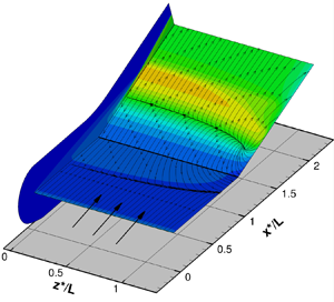
The three-dimensional grid was obtained by extruding the two-dimensional grid 100 mm in the spanwise direction, with 25 and 50 cells for grids Z1 and Z2, respectively, and a  $10\ \mathrm {\mu }\textrm {m}$ spacing imposed on the side of the model to capture spillage accurately. The difference between the results obtained with both grids is discussed in the grid-independence study. Grid Z2 was used for the remaining calculations. The far-field was reproduced with free-stream flow 25 mm away from the side of the model, with 25 cells used to calculate this region. An isometric perspective of a coarse version of the grid is given in figure 3.

Figure 3. Coarse version of the grid for the FSM with  $20^{\circ }$ and sharp leading-edge. Some surfaces have been removed for better visualisation.
4.1.2. Grid independence
Figure 4 shows the skin-friction coefficient and Stanton number distributions obtained with two-dimensional grids for the  $20^{\circ }$ case with sharp leading-edge and
  $T_w = 1050 \ \text {K}$. The non-dimensional coefficients of skin-friction, pressure and heat flux are defined as
 \begin{equation} C_f = \frac{\tau^*_w}{\frac{1}{2} \rho_{\infty} U_{\infty}^2}, \quad C_p = \frac{p^*_w}{\frac{1}{2} \rho_{\infty} U_{\infty}^2}, \quad St = \frac{q^*_w}{\rho_{\infty} U_{\infty} c_p (T_{ad} - T_w)}, \end{equation}
where  $T_{ad}$ is the adiabatic temperature and the superscript
  $*$ indicates dimensional quantities. The skin-friction peak is slightly smaller and closer to the corner for grid N1 compared with grids N2 and N3. Grids N2 and N3 provided results that collapsed on all points. For heat flux, all the three grids were seen to collapse on each other. Hence, it was considered that grid convergence was achieved with grid N2.

Figure 4. Skin-friction (a) and heat flux (b) coefficients for two-dimensional grids N1 (blue), N2 (green) and N3 (dark blue). N2 and N3 data collapse on all points.
Figure 5 shows the centreline distributions of skin-friction and heat flux coefficients for grids Z1 and Z2. The separation bubble is slightly smaller and both the skin-friction and heat flux peaks move slightly towards the corner with spanwise refinement. Because further refinement would be expected to provide little improvement and increased computational cost, grid Z2 was used for all three-dimensional cases. The centreline distributions of  $C_{f}, C_{p}$ and
  $St$ have been used throughout for comparison with the triple-deck results.

Figure 5. Skin-friction (a) and heat flux (b) coefficients for three-dimensional grids Z1 (blue) and Z2 (green).
4.2. Triple-deck calculations
4.2.1. Equations
One of the objectives of this paper is to compare the N–S solutions with those from triple-deck theory. The relevant equations are
 $$\begin{gather} \frac{\partial u}{\partial x} + \frac{\partial v}{\partial y} = 0, \end{gather}$$
 $$\begin{gather}\frac{\partial u}{\partial t} + u \frac{\partial u}{\partial x} + v \frac{\partial u}{\partial y} ={-} \frac{\partial p}{\partial x} + \frac{\partial^2 u}{\partial y ^2}, \end{gather}$$
and the interaction law
 \begin{equation} p ={-} \frac{\textrm{d} A}{\textrm{d}x} + \frac{\textrm{d} f}{\textrm{d}x}, \end{equation}
with boundary conditions
 $$\begin{gather} u = v = 0 \quad \text{at} \ y=0, \end{gather}$$
 $$\begin{gather}u \rightarrow y + A(x,t) \quad \text{as} \ \rightarrow \infty, \end{gather}$$
 $$\begin{gather}u \rightarrow y \quad \text{as}\ x \rightarrow - \infty, \end{gather}$$
where  $x$,
$x$,  $y$,
$y$,  $u$ and
  $v$ are the scaled non-dimensional streamwise and transverse dimensions and velocities in the lower deck, respectively, with the origin at the corner, and
  $p$ is the non-dimensional pressure as defined in Rizzetta et al. (Reference Rizzetta, Burggraf and Jenson1978). The function
  $f(x)$ describes the body shape. To smooth the region at the corner, the shape function is taken as
  $f(x) = {\alpha }/{2} (x + \sqrt {x^2 + r^2})$, where
  $\alpha$ is the scaled angle and
  $r$ is the rounding parameter, which is taken to equal
  $0.5$ unless otherwise stated.
4.2.2. Numerical procedure
The numerical procedure to solve these equations was that used by Cassel et al. (Reference Cassel, Ruban and Walker1995). Figure 6 shows the reproduction of the results of shear stress and pressure as a verification of implementation of their scheme.

Figure 6. Shear-stress (a) and pressure (b) distributions of supersonic flow over an adiabatic wall for different scaled angles (Cassel et al. Reference Cassel, Ruban and Walker1995). Blue, 1.0; green, 1.5; dark blue, 2.0; purple, 2.5; pink, 3.0; red, 3.5.
5. Results
5.1. Navier–Stokes results
5.1.1. Leading-edge region
Figure 7 shows the flow field around the leading-edge with wall temperature  $T_w = 300\ \textrm {K}$ and for the two leading-edge thicknesses. The bow shock is stronger with blunting, as would be expected. The bow shock is clearly detached with the blunt leading-edge but stays close to the tip of the model with the
  $40\ \mathrm {\mu }\textrm {m}$ leading-edge. The leading-edge shock is also stronger with increased blunting and leaves the model at a larger angle. The shock layer and the entropy layer were clearly distinguished in both cases.

Figure 7. Density gradient magnitude contours close to the leading-edge of the  $20^{\circ }$ FSM with
  $T_w=300\ \textrm {K}$. Leading-edge bluntness of
  $40\ \mathrm {\mu }\textrm {m}$ (a) and
  $200\ \mathrm {\mu }\textrm {m}$ (b).
5.1.2. Shock–shock interaction
Figure 8 shows the shock system around the domain for the  $20^{\circ }$ corner angle with sharp leading-edge and
  $T_w = 300\ \textrm {K}$. A leading-edge shock emerges from the tip of the model and travels above and below the model. For the
  $20^{\circ }$ case, a separation bubble sits at the corner and generates both a separation and a reattachment shock. The leading-edge shock coalesces with the reattachment shock at a triple-point, creating an Edney Type VI interaction. An expansion fan emerges from the triple-point and bounces against the wall. The same process takes place at the coalescence between the separation and reattachment shocks, thus two expansion fans impact the wall.

Figure 8. Shock structure for the  $20^{\circ }$ FSM with sharp leading-edge and
  $T_w=300\ \textrm {K}$.
The interaction of shock-waves downstream of the corner varies from case to case. For the  $10^{\circ }$ angle, separation occurs for wall temperature ratios above
  $s_w = 0.238$, but the separation bubble is too small to influence the shock-wave structure significantly. The conditions for incipient separation are considered in § 6.1. With the
  $20^{\circ }$ angle and both leading-edges, two types of shock interference take place. In the first type, the leading-edge and separation shock intersect the reattachment shock separately, producing two Edney Type VI interactions, as discussed earlier. In the second type, the leading-edge and the separation shock merge and intersect with the reattachment shock, resulting in a single triple-point. The second type of shock interference only takes place for the hottest wall
  $T_w =1050\ \textrm {K}$. The cold wall
  $T_w =300\ \textrm {K}$ manifests the first type and, as the wall temperature increases the separation point moves upstream of the corner, and the triple-point from the coalescence of the separation and reattachment shock moves downstream of the corner and eventually merges with the triple-point produced by the leading-edge and reattachment shock.
Clearly, the type of shock interference depends on the wall temperature. Figures 9 and 10 respectively show the influence of the first and second types of shock interference on the skin-friction distribution. The skin-friction coefficient is the wall parameter most affected because the expansion fan accelerates the flow close to the wall and increases the local shear-stress. For the first type of shock interference, two skin-friction maxima are observed on the ramp. They correspond to the impingement of the expansion fans that emerge from the triple-point. In figure 9, the second expansion fan is not visible because the leading edge shock is weak resulting in a weak expansion. In the second type of shock interference (figure 10), only one skin-friction maximum is obtained. Again, there is a clear relationship between the skin-friction peak and the shock structure in the interaction region.

Figure 9. First type of shock interference for the  $20^{\circ }$ FSM with sharp-leading edge (
 $40\ \mathrm {\mu }\textrm {m}$) and
  $T_w = 300\ \textrm {K}$. Density gradient magnitude contour (a) and skin-friction plot (b) in the shock–shock interaction region.

Figure 10. Second type of shock interference for the  $20^{\circ }$ FSM with sharp-leading edge (
 $40\ \mathrm {\mu }\textrm {m}$) and
  $T_w = 1050\ \textrm {K}$. Density gradient magnitude contour (a) and skin-friction plot (b) in the shock–shock interaction region.
5.1.3. Surface parameters
Figures 11–13 show N–S simulations of skin-friction, pressure and heat flux distributions for the  $10^{\circ }$ finite-span model for both sharp (
 $40\ \mathrm {\mu }\textrm {m}$) and blunt (
 $200\ \mathrm {\mu }\textrm {m}$) leading-edges. The results pertain to the symmetry plane.

Figure 11. Skin-friction coefficient distribution at the symmetry plane of the  $10^{\circ }$ FSM with (a)
  $40\ \mathrm {\mu }\textrm {m}$ and (b)
  $200\ \mathrm {\mu }\textrm {m}$ leading-edge bluntness. Cyan,
  $s_w = 0.095$; blue,
  $s_w = 0.143$; dark blue,
  $s_w = 0.190$; dark violet,
  $s_w = 0.238$; violet,
  $s_w = 0.286$; red,
  $s_w = 0.333$.
Considering figure 11, which shows the skin-friction, we see that prior to interaction upstream of the corner, the skin-friction is lower with blunting and higher with wall temperature. This trend reverses for the wall temperature downstream of the corner but remains the same with increased blunting. Separation seems to occur first at a wall temperature ratio of  $0.238$ and increases with further increase in wall temperature. The peak value of skin-friction on the ramp decreases with increasing wall temperature and increasing bluntness.
Figure 12 shows the pressure distribution for both sharp and blunt cases. Prior to interaction upstream of the corner, pressure increases with both blunting and increasing wall temperature. Downstream of the corner, the trend is reversed so that pressure decreases with both blunting and increase in wall temperature. The reduced ramp pressure with increased blunting is likely a result of loss of stagnation pressure at the leading-edge with a stronger bow shock. There is no discernible peak in the pressure, as observed in the skin-friction distribution.

Figure 12. Pressure coefficient distribution at the symmetry plane of the  $10^{\circ }$ FSM with (a)
  $40\ \mathrm {\mu }\textrm {m}$ and (b)
  $200\ \mathrm {\mu }\textrm {m}$ leading-edge bluntness. Cyan,
  $s_w = 0.095$; blue,
  $s_w = 0.143$; dark blue,
  $s_w = 0.190$; dark violet,
  $s_w = 0.238$; violet,
  $s_w = 0.286$; red,
  $s_w = 0.333$.
Figure 13 shows N–S simulations of the heat flux distribution for both sharp and blunt cases. Near the leading-edge, the wall temperature effects seem to be insignificant. At the corner, heat transfer is lower with the higher wall temperature and increased blunting. Both figures show the characteristic cusp-like shape at the corner indicative of attached flow, which is unlike the skin-friction plot of figure 11 that clearly shows separation at wall temperature ratios greater than  $s_w = 0.238$. This indicates that at higher temperatures, the flow is incipiently separating. The peak heating on the ramp decreases with blunting.

Figure 13. Stanton number distribution at the symmetry plane of the  $10^{\circ }$ FSM with (a)
  $40\ \mathrm {\mu }\textrm {m}$ and (b)
  $200\ \mathrm {\mu }\textrm {m}$ leading-edge bluntness. Cyan,
  $s_w = 0.095$; blue,
  $s_w = 0.143$; dark blue,
  $s_w = 0.190$; dark violet,
  $s_w = 0.238$; violet,
  $s_w = 0.286$; red,
  $s_w = 0.333$.
Figures 14–16 show the skin-friction, pressure and heat flux distributions for the  $20^{\circ }$ finite-span model for both sharp (
 $40\ \mathrm {\mu }\textrm {m}$) and blunt (
 $200\ \mathrm {\mu }\textrm {m}$) leading-edges.

Figure 14. Skin-friction coefficient distribution at the symmetry plane of the  $20^{\circ }$ FSM with (a)
  $40\ \mathrm {\mu }\textrm {m}$ and (b)
  $200\ \mathrm {\mu }\textrm {m}$ leading-edge bluntness. Cyan,
  $s_w = 0.095$; blue,
  $s_w = 0.143$; dark blue,
  $s_w = 0.190$; dark violet,
  $s_w = 0.238$; violet,
  $s_w = 0.286$; red,
  $s_w = 0.333$.
Figure 14 shows the skin-friction distribution for the finite-span model. A large separated region stretching upstream and downstream of the corner is evident. Looking at particular features, significant differences begin to appear from the beginning of interaction at approximately half way from the leading-edge. The separation extent (distance from separation to reattachment) increases with the increase in wall temperature and also increase in bluntness. Within the separated region, the shear-stress first increases slightly from the first minimum immediately following separation up to the corner, whereafter it falls sharply up to the second minimum before reattachment, which is typical of a moderate to large separated region (Gai & Khraibut Reference Gai and Khraibut2019). It is also noted that within this separated region, the flow is nearly independent of the wall temperature as well as bluntness.
Figure 15 shows the pressure distribution for the finite-span model. As in the  $10^{\circ }$ case, the pressure before interaction upstream of the corner is increasing with blunting and with the increase in wall temperature. The plateau pressure increases with increasing wall temperature but is not affected significantly by bluntness. The reattachment and peak pressures on the ramp increase with wall temperature and also seem independent of bluntness.

Figure 15. Pressure coefficient distribution at the symmetry plane of the  $20^{\circ }$ FSM with (a)
  $40\ \mathrm {\mu }\textrm {m}$ and (b)
  $200\ \mathrm {\mu }\textrm {m}$ leading-edge bluntness. Cyan,
  $s_w = 0.095$; blue,
  $s_w = 0.143$; dark blue,
  $s_w = 0.190$; dark violet,
  $s_w = 0.238$; violet,
  $s_w = 0.286$; red,
  $s_w = 0.333$.
Figure 16 shows the heat flux distribution for the finite-span model. Heat flux at the separation point shows a slight increase with wall temperature. This is also true inside the separated region except at the corner, where the trend reverses. Heat flux at reattachment shows a marked increase with wall temperature, but the peak heat flux decreases with wall temperature. With increased blunting, heat flux values are similar, except that the peak heat flux is smaller with increased blunting. The effect of the second expansion fan on the heat flux distribution downstream of reattachment is rather weak. Both figures are consistent with the separated region showing a well-rounded shape in the separated region and are consistent with the observation of Gadd (Reference Gadd1957a), where heat flux at separation is nearly independent of wall temperature ratio and that cooling (decreasing wall temperature ratio) makes the gradients at reattachment sharper and the separated region shorter.

Figure 16. Stanton number distribution at the symmetry plane of the  $20^{\circ }$ FSM with (a)
  $40\ \mathrm {\mu }\textrm {m}$ and (b)
  $200\ \mathrm {\mu }\textrm {m}$ leading-edge bluntness. Cyan,
  $s_w = 0.095$; blue,
  $s_w = 0.143$; dark blue,
  $s_w = 0.190$; dark violet,
  $s_w = 0.238$; violet,
  $s_w = 0.286$; red,
  $s_w = 0.333$.
5.2. Triple-deck results
Figure 17 shows the triple-deck solutions of the shear-stress and pressure obtained using the numerical procedure of Cassel et al. (Reference Cassel, Ruban and Walker1995) for the  $10^{\circ }$ compression corner, assuming a sharp-leading edge. Here, the differences in shear-stress with wall temperature, in terms of scaled angle, are much smaller than those in figure 11 based on the N–S solver. Note that the results in figure 17 are normalised in terms of the usual triple-deck notation. Separation occurs at
  $\alpha = 1.86$ (
 $s_w = 0.095$) compared with the N–S solution, which shows separation at
  $\alpha = 2.01$ (
 $s_w = 0.286$). Other significant features between the two solutions are that post-separation, the shear-stress distribution is unlike the CFD data, which show a maximum and then a slow reduction. This arises from shock interference effects discussed earlier which are not captured by the triple-deck solution. It should be pointed out that a characteristic of the triple-deck solution is that the viscous-inviscid process is modelled by the lower-deck incompressible boundary layer equations. Absence of any shock interaction is also evident in the investigation of the compression corner SBLI works of Korolev et al. (Reference Korolev, Gajjar and Ruban2002) and Cassel et al. (Reference Cassel, Ruban and Walker1995).

Figure 17. Shear-stress (a) and pressure (b) for the  $10^{\circ }$ case using the algorithm of Cassel et al. (Reference Cassel, Ruban and Walker1995), with
  $I = 201$,
  $J = 101$,
  $a = b = 5$. Cyan,
  $s_w = 0.095$; blue,
  $s_w = 0.143$; dark blue,
  $s_w = 0.190$; dark violet,
  $s_w = 0.238$; violet,
  $s_w = 0.286$; red,
  $s_w = 0.333$.
Figure 17 also shows the pressure distribution for the  $10^{\circ }$ case according to the triple-deck equations. Again, a comparison with N–S data of figure 12 shows that the effect of wall temperature is stronger on the ramp with the triple-deck solution. However, the pressures in the vicinity of the corner seem to be independent of the wall temperature unlike the N–S data, which show a somewhat smoother rise at higher temperatures. At the end of the ramp, while the triple-deck pressures maintain their differences (increasing pressure with increasing wall temperatures), the N–S simulations show coalescence independent of wall temperature.
Figure 18 shows the triple-deck solutions of shear-stress and pressure for the  $20^{\circ }$ compression corner. As in the
  $10^{\circ }$ case, the differences in shear-stress with wall temperature are smaller than those of figure 14 obtained with the N–S solver. In the separated region, the shear-stress decreases to the first minimum, then rises at the corner, and decreases again to the second minimum, similar to the N–S solution of figure 14. The effect of wall temperature is felt mostly at the second minimum, which decreases with increasing wall temperature, as in the N–S solution. No peaks are seen on the ramp in either the shear-stress or pressure distributions. This again arises from the absence of shock-waves in the triple-deck solution. It is interesting to note that the two shear stress minima in the triple-deck solution are sharper than the N–S solution, especially the second minimum. More importantly, at reattachment and after, the wall temperature seems to have negligible effect, which is quite different than the N–S solution. In figure 18(b), the pressures in the vicinity of the corner show much less variation with the wall temperature compared with the N–S solution. Downstream of the corner, an increase in wall temperature leads to an increase in the asymptotic pressure recovered on the ramp.

Figure 18. Shear-stress (a) and pressure (b) for the  $20^{\circ }$ case using the algorithm of Cassel et al. (Reference Cassel, Ruban and Walker1995), with
  $I = 101$,
  $J = 51$,
  $a = b = 5$. Cyan,
  $s_w = 0.095$; blue,
  $s_w = 0.143$; dark blue,
  $s_w = 0.190$; dark violet,
  $s_w = 0.238$; violet,
  $s_w = 0.286$; red,
  $s_w = 0.333$.
6. Discussion
6.1. Incipient separation
Based on experimental data obtained by various researchers (Ball Reference Ball1967; Hankey Reference Hankey1967; Needham Reference Needham1967), it has been shown that for cold wall hypersonic flows ( $T_w/T_0 < 1$), the incipient separation criterion can be expressed as
 \begin{equation} M \alpha_i^* = k \bar{\chi}^ {1/2}, \end{equation}
where the constant  $k$ varies in the range
  $1 \leq k \leq 1.3$. The other parameters in the above relation are the free stream Mach number
  $M$, the incipient separation angle
  $\alpha _i^*$ that causes separation and
  $\bar {\chi }$ is the hypersonic viscous interaction parameter.
As mentioned above, this relation is generally valid for cold surfaces. Stollery (Reference Stollery1972) proposed an expression for incipient separation, which includes wall temperature effects. The expression is
 \begin{equation} M \alpha_i^* = k \left( 1 - 0.5 s_w \right) \bar{\chi}^{1/2}, \end{equation}
where  $k$ is an empirical constant and
  $s_w$ is the wall temperature ratio. Based on experimental data, it is suggested that
  $k = 1.4$. Although not explicitly stated, the above relation assumes sharp leading-edge. The two leading edges being considered here can be taken as ’nominally sharp’ in terms of the criterion proposed by Stollery in the same paper.
In the present study, two compression corner angles of  $10^{\circ }$ and
  $20^{\circ }$ were chosen based on the estimate that
  $10^{\circ }$ would be nearer the incipient separation angle for the present free stream conditions. The
  $20^{\circ }$ angle was chosen to give a large separated region. Using the incipient separation criterion above, for the lowest wall temperature of
  $T_w = 300\ \textrm {K}$ and with a reservoir temperature of
  $T_0 = 3150\ \textrm {K}$, the incipient separation angle is
  $\alpha ^*_i = 11.3^{\circ }$. With an adiabatic wall, the incipient angle is
  $\alpha _i^* = 6.77^{\circ }$. These values are in excellent agreement with those of Neuenhahn & Olivier (Reference Neuenhahn and Olivier2012). For a
  $10^{\circ }$ incipient separation angle, the wall temperature ratio needs to be
  $s_w = 0.318$ (
 $T_w = 1000\ \textrm {K}$). This value is relatively close to the incipient separation wall temperature observed for the N–S results (wall temperature ratio between
  $s_w = 0.190$ and
  $s_w = 0.238$). The corresponding scaled angle for this wall temperature is
  $\alpha = 2.04$, which approximately agrees with the values listed in table 3. Using the relation
 \begin{equation} M \alpha_i^* = \alpha_i \lambda^{1/2} \bar{\chi}^{1/2}, \end{equation}
we can rewrite Stollery's formula as
 \begin{equation} \alpha_i = 2.43 ( 1 -0.5 s_w), \end{equation}
where  $\lambda$ is the Blasius shear constant with
  $\lambda = 0.332$. We note in passing that this does not involve the hypersonic viscous interaction parameter explicitly.
Table 3. Grid cells used in this study.

The above formula gives the scaled angle  $\alpha = 2.043$ for a wall temperature ratio of
  $s_w = 0.318$, which corresponds to a
  $10^{\circ }$ incipient separation angle as before. For an adiabatic wall, this relation gives the incipient value as
  $\alpha _i = 1.385$ instead of the value of
  $\alpha _i =1.57$ obtained by Rizzetta et al. (Reference Rizzetta, Burggraf and Jenson1978). This is because of the empirical constant
  $k = 1.4$ used by Stollery (Reference Stollery1972), which is based on experimental data. To yield Rizzetta's adiabatic value of
  $\alpha _i = 1.57$, Stollery's constant needs to be
  $k = 1.586$. It may be pointed out here that this adiabatic wall incipient separation value is quite close to the so called ‘true’ incipient separation value of
  $1.33$, as quoted by Grisham, Dennis & Lu (Reference Grisham, Dennis and Lu2018) based on an optimisation approach.
6.2. On the instability at the corner
In their triple-deck calculations, Cassel et al. (Reference Cassel, Ruban and Walker1995) observed a stationary wave-packet located at the corner of the compression ramp for scaled angles  $\alpha \geq 3.9$. They attributed this to absolute instability as it remained stationary and did not convect downstream. It was also found to be highly mesh-dependent. The wave-packet was invariant with respect to shape and streamwise extent irrespective of mesh size. The corresponding velocity profiles showed an inflection point and satisfied both Rayleigh and Fjørtoft criteria for instability. Fletcher, Ruban & Walker (Reference Fletcher, Ruban and Walker2004) further explored this instability using the same algorithm as that of Cassel et al. (Reference Cassel, Ruban and Walker1995). They obtained steady stable solutions for small scaled angles but for sufficiently large scaled angles,
  $\alpha = 3.7$, absolute instability was seen to occur. They also found that while the absolute instability was bounded for
  $\alpha = 3.7$, it was unbounded for
  $\alpha =4.2$. In addition, in the range
  $3.2 \leq \alpha \leq 3.7$, convective instabilities were observed and were attributed to the interpolation process towards a finer grid or to an external disturbance imposed on a steady state. Logue, Gajjar & Ruban (Reference Logue, Gajjar and Ruban2014), who analysed the supersonic compression corner problem using the unsteady triple-deck equations, but using different numerical approaches, did not encounter this instability problem for a range of scaled angles from
  $3$ to as high as
  $7.5$. Logue et al. (Reference Logue, Gajjar and Ruban2014, p. 11) conclude: ‘Our unsteady results have shown that despite using a number of different robust numerical techniques, the precise mechanisms causing breakdown of the unsteady supersonic compression ramp flow, governed by the triple deck equations, still remain unclear.’ It should, however, be pointed out in this connection that Smith (Reference Smith1988a,Reference Smithb) has discussed the unsteady interactive boundary layer and separation breakdown at a localised discontinuity based on the triple-deck theory.
From the above discussion, it is quite evident that the reason, whether physical or numerical, for the spontaneous appearance of this instability at certain higher scaled angles is still unresolved. Given that the supersonic free stream is uniform and two-dimensional, the obvious possible reason could be the geometry of the ramp, particularly the corner discontinuity. All the previous authors (except Smith & Khorrami Reference Smith and Khorrami1991) assume a shape function
 \begin{equation} f(x) = \frac{\alpha}{2} \left( x + \sqrt{ x^2 + r^2} \right), \end{equation}
where  $r$ is the so-called rounding factor introduced to smoothen the discontinuity at the corner. All the above studies have used
  $r = 0.5$ in their computations. While they have experimented with various mesh sizes depending on the numerical method used, there has not been a detailed investigation of the effect of
  $r$ on computations, although Cassel et al. (Reference Cassel, Ruban and Walker1995) state that
  $r$ does have significant influence on the ramp angle at which separation first occurs (incipient separation) and that once separation occurs, its influence is minimal. Korolev et al. (Reference Korolev, Gajjar and Ruban2002) point out that when separation is large and the corner is deeply embedded in the low-velocity reverse-flow region, the differences in the results between a sharp corner and a rounded corner become indistinguishable. To verify these assumptions, we show some results with varying
  $r$.
$r$.
The shape function influences the numerical results through coefficient  $\bar {d}_i$ (Cassel et al. Reference Cassel, Ruban and Walker1995), which includes the second-order derivative
  $\textrm {d}^2 f / {\textrm {d}x}^2$. At the corner,
 \begin{equation} \left.\frac{ \textrm{d}^2 f}{{\textrm{d}x}^2} \right|_{x =0} = \frac{1}{2} \frac{\alpha}{r}, \end{equation}
where  $r$ is the non-dimensional radius at the corner.
This expression shows that  $\textrm {d}^2 f / {\textrm {d}x}^2$ is quite sensitive to the value of
  $r$ for a given
  $\alpha$ and when
  $r \ll 1$ would likely affect the stability of the algorithm through (6.6).
Figures 19(a) and 19(b) illustrate the effect of a small  $r$ compared with
  $r = 0.5$ used in previous investigations for two scaled angles using a coarse mesh. We note (figure 19a) that even with a coarse mesh, a weak wave-packet occurs for a scaled angle as low as
  $2.0$ when a small separation has just occurred. Note that Cassel et al. (Reference Cassel, Ruban and Walker1995) observed incipient separation at a scaled angle of
  $1.9$ instead of
  $1.57$ (Rizzetta et al. Reference Rizzetta, Burggraf and Jenson1978) and attributed this to the ‘smoothed corner.’ Therefore, it is possible that the weak wave-packet seen in figure 19(a) arises from the effect of a small radius in a small separated region. It is also consistent with the observation of Korolev et al. (Reference Korolev, Gajjar and Ruban2002), where smoothing should alleviate the corner effect in large separated regions.

Figure 19. Wave-packet at the corner for the scaled angle  $\alpha = 2.0$ (a) and
  $\alpha = 3.0$ (b) with non-dimensional radius
  $r = 0.05$, with
  $I = 101$,
  $J = 51$ and
  $a = b = 5$, at
  $t = 85$.
When the scaled angle is increased to  $3.0$ (figure 19b), the wave-packet is sharper with larger amplitude and is firmly stationed at the corner. With both scaled angles
  $\alpha = 2.0$ and
  $\alpha = 3.0$,
  $\textrm {d}^2 f / {\textrm {d}x}^2$ is an order of magnitude larger than that used in earlier investigations. Now, figure 20(a) shows the situation for
  $\alpha = 3.0$ with
  $I = 601$,
  $J = 101$,
  $a = b= 5$ and
  $r =0.05$. We note that with a finer mesh, the oscillations are smoothed out considerably and show smaller amplitudes. The same features are seen for
  $\alpha =3.5$ with the same mesh and radius
  $r$. This is consistent with the observations of Fletcher et al. (Reference Fletcher, Ruban and Walker2004), who found that in the range
  $3.2 \leq \alpha \leq 3.7$, the flow was in a convectively unstable state in the separated region in the vicinity of the corner, which they attributed principally to the interpolation process towards a finer grid. These results would, therefore, indicate that wave-packets at the corner seem more a manifestation of numerical difficulty, which seems particularly sensitive to mesh size and the process of smoothing of the corner discontinuity through the shape function. This corner singularity does not seem to have been a serious issue in the study by Smith & Khorrami (Reference Smith and Khorrami1991), who used the shape function
  $f(x) = \alpha x / [ 1 + \exp (-q x)]$, where
  $q$ is a large positive constant. It is also noted by these authors that the effect of smoothing did not affect the flow field away from the vicinity of the corner. Likewise, Rizzetta et al. (Reference Rizzetta, Burggraf and Jenson1978) also do not mention any particular difficulties with corner singularity except to say that the singularity in shear-stress was resolved on a length scale smaller than that of the triple deck.

Figure 20. Wave-packet at the corner for the scaled angle  $\alpha = 3.0$ (a) and
  $\alpha = 3.5$ (b) with non-dimensional radius
  $r = 0.05$, with
  $I = 601$,
  $J = 101$ and
  $a = b = 5$, at
  $t = 85$.
To explore this problem further, we undertook a parametric study using the mesh size, the non-dimensional radius of the corner  $r$ and the scaled angle
  $\alpha$. Two mesh sizes
  $(I,J) = (101,51)$ and
  $(I,J) = (201,51)$ were used. Only points in the streamwise direction were increased, as this is shown to be critical in inducing instability (Fletcher et al. Reference Fletcher, Ruban and Walker2004). The non-dimensional radius
  $r$ was set at
  $r = 0.05$. Calculations were carried out for
  $1.0 \leq \alpha \leq 1.5$ with the coarse mesh, and the results are shown in figure 21. We see the beginning of a wave-packet soon after
  $\alpha =1$ and by
  $\alpha = 1.5$, a full wave-packet is formed. Even at
  $\alpha =1$, separation is indicated. Obviously, the results are grid-dependent and inaccurate. Interestingly, these results seem contrary to those of Cassel et al. (Reference Cassel, Ruban and Walker1995), where no wave-packets were observed for
  $1.0 \leq \alpha \leq 3.5$ with the mesh size
  $(I,J) = (101,51)$ but
  $r =0.5$. With the mesh size increased to
  $(I,J) = (201,51)$, the wave-packet appears at slightly larger scaled angles. Figure 21 shows the wave-packet with this mesh, for
  $1.5 \leq \alpha \leq 2.0$ and
  $r =0.05$, where we see slight improvement in the results. Incipient separation now clearly occurs around scaled angles
  $1.5$ and
  $1.6$, in agreement with Rizzetta et al. (Reference Rizzetta, Burggraf and Jenson1978). A wave-packet has formed by
  $\alpha = 2.0$. These data clearly show the strong effect of the non-dimensional radius apart from the mesh size.

Figure 21. Evolution of the wave-packet at the corner for scaled angles  $(a1)$
  $\alpha = 1.0$ and
  $(b1)$
  $\alpha = 1.5$ with
  $I = 101$,
  $J = 51$, and
  $(a2)$
  $\alpha = 1.5$ and
  $(b2)$
  $\alpha = 2.0$ with
  $I = 201$,
  $J = 51$. Parameters:
  $a = b = 5$;
  $r = 0.05$;
  $t = 85$.
To further confirm the strong influence of the shape function, we performed calculations using the shape function used by Smith & Khorrami (Reference Smith and Khorrami1991), which yields  ${\textrm {d}^2 f}/{{\textrm {d}x}^2} |_{x=0} = \alpha q /2$.
This is quite similar to the expression obtained from the shape function used by Cassel et al. (Reference Cassel, Ruban and Walker1995), wherein  $\textrm {d}^2 f / {\textrm {d}x}^2 |_{x=0} = \alpha / 2r$ so that
  $q$ corresponds to
  $1/r$. Thus, the value
  $q = 20$ used by Smith & Khorrami (Reference Smith and Khorrami1991) is equivalent to
  $r = 0.05$. Repeating the calculations with the shape function used by Smith & Khorrami (Reference Smith and Khorrami1991), we get the results shown in figure 22 for the coarse mesh
  $(101,51)$,
  $q = 20$, and
  $1.5 \leq \alpha \leq 2.0$. It is seen that starting as a small discontinuity at
  $\alpha =1.5$, a fully developed wave-packet has evolved by
  $\alpha = 2.0$. As with the shape function of Cassel et al. (Reference Cassel, Ruban and Walker1995), the discontinuity at the corner develops into a wave-packet with the increase in scaled angle. Figure 22 also shows results for scaled angles from
  $2.0$ to
  $2.5$ but with a finer mesh
  $(201,51)$. Smith & Khorrami (Reference Smith and Khorrami1991), using this shape function, did not encounter such a wave-packet for scaled angles up to
  $6.6$. Because Smith & Khorrami (Reference Smith and Khorrami1991) solved the triple-deck equations with the same shape function but a different numerical algorithm, results obtained here appear to arise from the particular numerical scheme of Cassel et al. (Reference Cassel, Ruban and Walker1995), which was also used in the present instance. We believe, therefore, that there is no physical basis for the existence of a wave-packet, as proposed in Cassel et al. (Reference Cassel, Ruban and Walker1995).

Figure 22. Evolution of the wave-packet at the corner with the shape function of Smith & Khorrami (Reference Smith and Khorrami1991) for scaled angles  $(a1)$
  $\alpha = 1.5$ and
  $(b1)$
  $\alpha = 2.0$ with
  $I = 101$,
  $J = 51$, and
  $(a2)$
  $\alpha = 2.0$ and
  $(b2)$
  $\alpha = 2.5$ with
  $I = 201$,
  $J = 51$. Parameters:
  $a = b = 5$;
  $r = 0.05$;
  $t = 85$.
6.3. Secondary vortices
Computations were carried out with scaled angles of  $\alpha = 4.5$ and
  $\alpha = 5.0$ to compare the data with those of Korolev et al. (Reference Korolev, Gajjar and Ruban2002) and Smith & Khorrami (Reference Smith and Khorrami1991). The parameters used were
  $I = 101$,
  $J = 51$,
  $a = b = 5$,
  $r = 0.5$, the domain was extended to
  $y_M = 120$ and the solutions obtained at
  $t = 180$. The coarse mesh was used to suppress any possibility of instability at the corner (see Cassel et al. Reference Cassel, Ruban and Walker1995) at higher scaled angles. Figures 23 and 24 show the results.

Figure 23. Shear-stress (a) and pressure (b) for scaled angle  $\alpha = 4.5$, with
  $a = b = 5$,
  $I = 101$,
  $J = 51$.

Figure 24. Shear-stress (a) and pressure (b) for scaled angle  $\alpha = 5.0$, with
  $I = 101$,
  $J = 51$,
  $a = b = 5$.
Considering the shear-stress (figure 23a), a large separated region with two minima is seen, and upstream of the corner, the shear-stress is unity before decreasing as separation is approached at  $x = -12.16$. Correspondingly, the pressure rises from
  $p=0$ to separation before attaining an extended plateau (figure 23b). The shear-stress increases as the corner is approached and is on the verge of zero, which indicates that a secondary separation is about to occur. The second minimum immediately follows past the corner before reattachment occurs at
  $x = 8.49$. The indication of a dip in pressure in the vicinity of the corner at the end of the plateau is also an indication that a secondary separation is imminent (Smith & Khorrami Reference Smith and Khorrami1991; Korolev et al. Reference Korolev, Gajjar and Ruban2002). When this occurs, the pressure gradient becomes very large and the second minimum in shear stress follows prior to reattachment (Smith Reference Smith1988b). Figure 25(a) shows velocity contours close to the corner. A large single separation bubble is seen largely centred towards the ramp side. The results show excellent agreement with those of Korolev et al. (Reference Korolev, Gajjar and Ruban2002) for
  $\alpha = 4.5$. Agreement with the data of Smith & Khorrami (Reference Smith and Khorrami1991) for the same scaled angle is equally good.

Figure 25. Velocity contours for scaled angles  $\alpha = 4.5$ (a) and
  $\alpha = 5.0$ (b), with
  $I = 101$,
  $J = 51$,
  $a = b = 5$.
Figure 24 shows the results for  $\alpha =5.0$. We note that apart from the larger separated region, a secondary separation has now developed, as indicated by the positive shear-stress between
  $x = -1.23$ and
  $x = 3.03$, before reaching a sharp minimum (the second minimum) immediately prior to reattachment. The separation and reattachment are located at
  $x_{sep} = -14.29$ and
  $x_{reat} = 9.00$, respectively. Figure 24(b) shows the pressure distribution with a large plateau and a steep drop in pressure at the end of the plateau, which indicates the secondary separation begins slightly ahead of the corner. The reattachment region is characterised by a sharp rise in pressure. The possible theoretical implications of flow features, such as the appearance of the second minimum in shear stress and the accompanying pressure gradients, are discussed by Smith (Reference Smith1988a,Reference Smithb).
Figure 25(b) shows the streamlines with velocity contours in the separated region. Embedded within the main recirculation region is a secondary separation bubble located along the ramp surface. Again, these results are in very good agreement with both those of Korolev et al. (Reference Korolev, Gajjar and Ruban2002) and Smith & Khorrami (Reference Smith and Khorrami1991). In passing, it is interesting to note that the secondary bubble structure and location are similar to those of Korolev et al. (Reference Korolev, Gajjar and Ruban2002) but unlike the N–S-based solutions of Shvedchenko (Reference Shvedchenko2009) and Gai & Khraibut (Reference Gai and Khraibut2019), where secondary bubbles are predominantly located upstream of the corner.
6.3.1. Velocity and curvature profiles in the separated region
Figures 26 and 27 show profiles of velocity and curvature ( $\partial ^2 u / \partial y^2$) at locations ahead of separation (
 $x = -31.57$), after separation (
 $x = -4.27$), at the corner (
 $x =0$) and before reattachment (
 $x = 4.27$) for the two scaled angles
  $\alpha = 4.5$ and
  $\alpha = 5.0$, respectively. Considering the velocity profiles in figure 26(a) first, the profile ahead of separation
  $(x = -31.57)$ is seen to be linear while the two profiles in the separated region (
 $x = \pm 4.27$) are typical reverse-flow profiles. The profile at the corner shows a large reverse-flow region compared with the other two profiles. These three reverse-flow profiles give an indication of how the separation size increases and how the velocity varies near the surface. Figure 26(b) shows the curvature profiles and one can see inflection points for the corner profile prior to reattachment (
 $x = 4.27$). Interestingly, the profile immediately after separation (
 $x = -4.27$) does not show an inflection. This is similar to the observation of Cassel et al. (Reference Cassel, Ruban and Walker1995), who found that reverse flow is possible without the appearance of an inflection point. It is also pointed out that while Cassel et al. (Reference Cassel, Ruban and Walker1995) found no inflection point on the corner profile for
  $\alpha = 3.5$, in the present instance, such a profile is seen at
  $\alpha = 4.5$.

Figure 26. Velocity (a) and  $\partial ^2 u / \partial y^2$ (b) profiles for
  $\alpha = 4.5$, with
  $I = 101$,
  $J = 51$
  $a = b = 5$. Red,
  $x = -31.57$; green,
  $x=-4.27$; blue,
  $x =0$; black,
  $x = 4.27$.

Figure 27. Velocity (a) and  $\partial ^2 u / \partial y^2$ (b) profiles for
  $\alpha = 5.0$, with
  $I = 101$,
  $J = 51$,
  $a = b = 5$. Red,
  $x = -31.57$; green,
  $x=-4.27$; blue,
  $x =0$; black,
  $x = 4.27$.
Figure 27 shows the velocity and curvature profiles for  $\alpha = 5.0$. The velocity profiles (figure 27a) are largely similar to those of
  $\alpha = 4.5$ except that the corner profile shows a small positive velocity near the surface, which indicates secondary separation. We also note that the separation is larger. Again, the curvature profiles (figure 27b) are similar to those of
  $\alpha = 4.5$ except that inflection points are located further away from the surface and also that the profile at
  $x = -4.27$ shows, for the large part,
  $\partial ^2 u / \partial y^2 > 0$ before going to zero at the surface to satisfy the no-slip condition.
6.4. Wall temperature effects
Analyses by Brown et al. (Reference Brown, Cheng and Lee1990), Kerimbekov et al. (Reference Kerimbekov, Ruban and Walker1994) and Cassel et al. (Reference Cassel, Ruban and Walker1996) have considered wall cooling effects on the separation using triple-deck approach. These analyses delineate the wall temperature effects into subcritical, transcritical and supercritical regimes, as discussed in § 2.
The triple-deck calculations from the present investigations are shown in figure 18 for shear-stress distributions obtained for the  $20^{\circ }$ compression corner with
  $I = 201$,
  $J = 101$,
  $a = b= 5$,
  $r =0.5$.
These results agree quite well with the trends seen by Cassel et al. (Reference Cassel, Ruban and Walker1996). There is a steep drop in the shear-stress from  $\tau _w = 1$ to zero at separation but the fall is less abrupt compared with that observed by Cassel et al. (Reference Cassel, Ruban and Walker1996). The separation extent also becomes less with a decrease in wall temperature. The small increase in shear-stress in the recirculation region near the corner shows that the increase is higher with the higher wall-temperature, again as in the data of Cassel et al. (Reference Cassel, Ruban and Walker1996). The small oscillations immediately before separation, observed by Cassel et al. (Reference Cassel, Ruban and Walker1996), are not seen. This is because the cooling effects in the present instance are comparatively moderate compared with those considered by Cassel et al. (Reference Cassel, Ruban and Walker1996). With the hotter wall, the separation increases by nearly
  $21\,\%$.
Figures 28–30 show velocity profiles and their derivatives at different locations: at separation; at the corner ( $x=0$); and at reattachment, for the
  $20^{\circ }$ case with cold (
 $s_w = 0.095$) and hot (
 $s_w = 0.333$) walls. Considering the profiles of the colder wall (
 $s_w = 0.095$) at separation (
 $x = -7.98$), the curvature profile shows a maximum near the surface where the velocity is changing rapidly near the surface from zero. All the three parameters go to zero at the surface to satisfy the no-slip boundary condition. Away from the surface, the curvature shows zero when the velocity profile is nearly linear. These features are similar to those for the hotter wall (
 $s_w =0.333$) at
  $x =-10.25$.

Figure 28. Velocity and derivative profiles for  $s_w = 0.095$ (a) and
  $s_w = 0.333$ (b) at separation points
  $x = -7.98$ and
  $x = -10.25$, for
  $\alpha = 3.72$ and
  $\alpha = 4.13$, respectively.
Considering the corner profiles for the colder wall ( $s_w = 0.095$), the velocity profile shows a highly reverse flow and the curvature profile (
 $\partial ^2 u / \partial y^2$) shows a maximum near the surface before going to zero away from the surface when the velocity variation is nearly linear away from the surface. The vorticity
  $\partial u / \partial y$ profile shows negative vorticity at the surface corresponding to the reverse-flow and crosses zero at the maximum reverse velocity point and stays approximately constant at sufficient distance away from the surface. In the corner profiles for the hotter wall (
 $s_w =0.333$), there are some significant differences. First, the profiles are less full. In the velocity profile, the velocities close to the surface are decreased and are much straighter than those for the colder wall, a feature also noted by Cassel et al. (Reference Cassel, Ruban and Walker1995) for a higher scaled angle. This is reflected in the curvature (
 $\partial ^2 u / \partial y^2$) profile being zero, unlike in the cold wall case, and there may even be an inflection point very close to the surface (see Cassel et al. Reference Cassel, Ruban and Walker1995). Note that both the scaled angles for the colder and hotter walls in the present case are
  $3.72$ and
  $4.13$, respectively. This is consistent with the observation of Cassel et al. (Reference Cassel, Ruban and Walker1995) that when the scaled angle
  $\alpha \leq 3.9$, an inflection point is not likely even in the presence of separation.
The vorticity profile ( $\partial u / \partial y$) shows that the vorticity at the surface is also less for the hotter wall and changes sign further away from the surface. The zero crossing of vorticity coincides with the maximum of the reverse-flow velocity similar to the cold wall case.
The profiles at reattachment are very similar to those at separation and the differences between hotter and colder walls are less stark.
Noteworthy features of the curvature profiles are that  $\partial ^2 u / \partial y^2$ is mostly positive throughout in all the cases and although velocity profiles show reverse flow, there is no discernible inflection point even with the hotter wall.

Figure 29. Velocity and derivative profiles for  $s_w = 0.095$ (a) and
  $s_w = 0.333$ (b) at the corner
  $x=0$, for
  $\alpha = 3.72$ and
  $\alpha = 4.13$, respectively.

Figure 30. Velocity and derivative profiles for  $s_w = 0.095$ (a) and
  $s_w = 0.333$ (b) at reattachment points
  $x = 7.05$ and
  $x = 7.92$, for
  $\alpha = 3.72$ and
  $\alpha = 4.13$, respectively.
6.5. Separation length
Figure 31(a) shows the effect of wall temperature and bluntness on separation length  $L_s$ normalised by the flat plate length
  $L$ (up to the corner). It has been shown that, in terms of the criteria of Stollery (Reference Stollery1972) and Lagrée (Reference Lagrée1991), both bluntness values of
  $40\ \mathrm {\mu }\textrm {m}$ and
  $200\ \mathrm {\mu }\textrm {m}$ can be considered 'small’. However, as seen from this figure, there are significant differences between them with the wall temperature. First, the higher bluntness induces larger separation for a given wall temperature ratio. Second, variations with wall temperature are nearly linear for both bluntness cases.

Figure 31. (a) Effect of wall temperature and bluntness on separation length (red,  $40\ \mathrm {\mu }\textrm {m}$; black,
  $200\ \mathrm {\mu }\textrm {m}$). (b) Comparison of separation length with triple-deck (blue) and N–S (black) solutions.
One of the conclusions of Katzer (Reference Katzer1989) is that for finite Reynolds numbers, the triple-deck theory tends to over-predict the size of the separation bubble. It is, therefore, of interest to compare the length of the separation bubble obtained from both triple-deck and N–S solutions. Figure 31(b) shows the separation length plotted against the wall temperature ratio  $s_w$. The bubble length, in terms of triple-deck scaling, can be determined using the relations in Rizzetta et al. (Reference Rizzetta, Burggraf and Jenson1978) or Katzer (Reference Katzer1989). The corresponding N–S values were determined from the solutions described in § 5.1. It is seen that the triple-deck separation length overpredicts the corresponding N–S values for
  $s_w \geq 0.15$ and the difference increases substantially with the increase in wall temperature. However, for
  $s_w \leq 0.15$, the reverse happens, that is, the triple-deck theory underpredicts the N–S value. The reason, as pointed out by Brown et al. (Reference Brown, Khorrami, Neish and Smith1991), is that for highly cooled walls, the lower deck dimension is drastically reduced and consequently both separation and the upstream influence are much reduced. This is also in line with the observations of Nielsen et al. (Reference Nielsen, Lynes and Goodwin1966), who found that both interaction length and separation were vanishingly small for wall temperature ratios less than
  $0.133$. The present data are consistent with the above observations. It should be pointed out that while the N–S data pertain to finite Reynolds number and finite-span geometry, the triple-deck is a two-dimensional asymptotic approximation.
6.6. Finite-span effects
The critical point theory of Legendre et al. (Reference Legendre1977) provides a consistent language to analyse the three-dimensional flow structure. Separation and reattachment points obtained at every  $x$–
$x$– $y$-plane fall on lines named the separation and reattachment lines, respectively (Delery Reference Delery1992; Babinsky & Harvey Reference Babinsky and Harvey2011). A separation node can be identified when skin-friction lines converge towards one point, while an attachment node displays skin-friction lines diverging from it. Figure 32 shows the pressure coefficient contours over the wall for the
  $20^{\circ }$ finite-span model with a
  $40\ \mathrm {\mu }\textrm {m}$ leading-edge and
  $T_w = 1050\ \textrm {K}$. The flow remains two-dimensional at the centreline. The flow structure is similar to that reported by Rudy et al. (Reference Rudy, Thomas, Kumar, Gnoff and Chakravarthy1989). The separation follows a curved line from the symmetry plane towards the edge of the model. The separation bubble is thus larger at the centreline than at the edge of the wall. The skin-friction lines indicate significant outflow in the spanwise direction at the side of the plate. This arises from the spillage of flow from the top of the model towards the free stream. An attachment node can be seen close to the edge of the plate. The skin-friction lines at reattachment emerge from this node and travel both downstream and slightly towards the centreline and, like the separation line, the reattachment line is also curved with the apex at the centreline. Far from the side of the wall, the flow on the ramp remains two-dimensional.

Figure 32. Isometric view of wall pressure coefficient contours for the  $20^{\circ }$ FSM with
  $40\ \mathrm {\mu }\textrm {m}$ leading-edge and
  $T_w = 1050\ \textrm {K}$.
The scaled angles for the  $20^{\circ }$ case range from
  $\alpha = 3.7$ to
  $\alpha = 4.1$. Two-dimensional N–S simulations from several authors suggest the existence of secondary vortices for this range of scaled angle values (Shvedchenko Reference Shvedchenko2009; Egorov et al. Reference Egorov, Neiland and Shredchenko2011; Gai & Khraibut Reference Gai and Khraibut2019). The absence of such vortices in the present simulations might be due to three-dimensional effects. However, the aspect ratio of the model considered here is larger than unity, and the flow on the centreline remains two-dimensional. Furthermore, previous triple-deck literature (Smith & Khorrami Reference Smith and Khorrami1991; Korolev et al. Reference Korolev, Gajjar and Ruban2002) does not predict secondary vortices for scaled angles lower than
  $\alpha = 4.5$, as shown earlier. It is therefore unresolved as to why secondary vortices are not seen in our N–S calculations.
7. Conclusions
Wall temperature and bluntness effects can influence both the flow field structure and surface parameters. In respect of the flow field, wall temperature influences the mode of shock interference. For a cold wall, the leading-edge shock and separation shock intersect the reattachment shock separately resulting in two Edney Type VI interactions with two triple points and two expansion fans which reflect off the ramp surface. This results in two maxima in the skin-friction distribution on the ramp surface. As the wall temperature increases, the separation point moves upstream and the triple point, produced by the intersection of separation and reattachment shocks, moves downstream of the corner. This triple point eventually merges with the triple point produced by the leading-edge and the reattachment shocks at the hottest wall temperature considered in this study ( $T_w = 1050\ \textrm {K}$). As a consequence, only one maximum is seen in the skin-friction distribution on the ramp surface. The pressure distributions show peaks and steep drops consistent with these shock interference patterns.
Wall temperature has a significant impact on separation. The criterion of Stollery (Reference Stollery1972) predicts incipient separation at a wall temperature ratio of  $0.318$ for a
  $10^{\circ }$ corner angle. For the same angle, the N–S solution predicts incipient separation at wall temperature ratio between
  $0.190$ and
  $0.238$ for the finite-span model. The two-dimensional triple-deck solution for an adiabatic wall showed incipient separation to occur at a scaled angle
  $\alpha = 1.86$, which is in good agreement with that of Cassel et al. (Reference Cassel, Ruban and Walker1995), who found incipient separation at
  $\alpha \approx 1.9$ for a compression corner at supersonic Mach numbers.
Both wall temperature and bluntness increased the separation length. For  $s_w \geq 0.15$, the triple-deck overpredicts the N–S solution while for
  $s_w \leq 0.15$, the opposite is true. Overall, the effect of wall temperature on separation length was found to be much greater with triple-deck solution than that with the N–S. The effects of wall temperature and bluntness are minimal within the separated region.
The instability at the corner in the form of a stationary wave packet noted by Cassel et al. (Reference Cassel, Ruban and Walker1995) for scaled angles  $\alpha \geq 3.9$ is shown to be a manifestation of a numerical artefact in the algorithm, which seems to be particularly sensitive to both mesh size and the corner shape function. With coarse mesh and small rounding radius, the wave packet could be suppressed for scaled angles up to
  $\alpha = 5$. The results for these scaled angles are in excellent agreement with those of Smith & Khorrami (Reference Smith and Khorrami1991) and Korolev et al. (Reference Korolev, Gajjar and Ruban2002).
Results from the finite-span model (FSM) showed that three-dimensional effects are largely confined near edges and the flow over the midspan region could be taken as nominally two-dimensional. The flow structure compares well with the three-dimensional solutions of Rudy et al. (Reference Rudy, Thomas, Kumar, Gnoff and Chakravarthy1989). Secondary vortices were not observed in the present investigation despite the fact that the scaled angles varied from  $3.72$ to
  $4.12$. This is contrary to Shvedchenko (Reference Shvedchenko2009) and Gai & Khraibut (Reference Gai and Khraibut2019), who observed secondary separation for scaled angles
  $3 \leq \alpha \leq 4$. This is believed to be due to the finite span of the model in the present investigation.
Acknowledgements
The authors would like to thank Professor G. Candler from the University of Minnesota for access to the US3D solver. Numerical resources were provided by the National Computational Infrastructure (NCI) under the NCMAS scheme, which is supported by the Australian Government. We would also like to thank the referees for their helpful comments and suggestions.
Funding
This study has been funded by the Air Force Office of Scientific Research (AFOSR) under grant number FA238619-1-4023 and we would like to thank Dr R. Carr for his interest and advice.
Declaration of interests
The authors report no conflict of interest.


