


1 Introduction
Breakup of a time-varying cylindrical blob represents a key example of the evolution of a perturbation superimposed on a time-dependent base state and arises in various situations, such as edges of retracting soap films, extending fluid threads and stretching liquid bridges. Historically, proper stability analysis of time-dependent base states has often been obstructed by the difficulties associated with analytical treatment, apart from very few scarce exceptions when there is symmetry (Plesset Reference Plesset1954) or periodicity (Davis Reference Davis1976), and is therefore most frequently amenable to numerical methods only (Homsy Reference Homsy1973). Without exception, stability analysis of a growing blob has hitherto been based on either phenomenological (i.e. not exact) formulations or numerical simulations (cf. Fullana & Zaleski (Reference Fullana and Zaleski1999), Roisman, Horvat & Tropea (Reference Roisman, Horvat and Tropea2006), Agbaglah, Josserand & Zaleski (Reference Agbaglah, Josserand and Zaleski2013), Dziwnik et al. (Reference Dziwnik, Korzec, Münch and Wagner2014), to name a few), often producing contradictory results and thus calling for a precise analysis to be performed. Explicit in many of these studies is the universal assumption that the instability can be described by spectra (eigenvalues) of the corresponding autonomous linear operator, usually enabled by a ‘frozen’ base state, resulting in exponential growth of the perturbation. A somewhat different formulation by Dziwnik et al. (Reference Dziwnik, Korzec, Münch and Wagner2014), based on a thin-film approximation, which strictly speaking is invalid in the rim region and in which the initial fronts evolve slower compared with their instability, thus allowing a time-scale separation, envisaged the idea of a time-dependent dominant wavelength that scales with the size of the growing rim.
As will be shown in the present study (§ 3), the assumption of exponential growth proves to be inadequate in the context of a growing rim if its (base sate) radius varies on the same time scale as instability. Moreover, the results of the analysis of the original fluid dynamics equations (§§ 2–3) suggest that the phenomenological equations fail to capture the true intricacies of the instability dynamics. It is also demonstrated that the seemingly intuitive idea of a time-dependent wavenumber scaling with the time-dependent rim radius is not mathematically justified (§ 3). For an analytical study of the instability of an accelerating cylindrical blob in the large-Bond-number regime, when its growth in time is treated in a quasi-steady fashion (i.e. instability develops faster than the initial cylindrical base state is modified), the reader is referred to Krechetnikov (Reference Krechetnikov2010). In the present work, we consider the opposite situation, namely when the time dependence of the base state (growing cylinder) cannot be neglected, but the effect of the lateral acceleration
 $g$
is treated as a perturbation in the limit of small Bond number.
$g$
is treated as a perturbation in the limit of small Bond number.
2 Derivation of the linear stability equations
The problem of breakup of a liquid jet is often studied in the incompressible inviscid potential approximation, starting with the work of Rayleigh (1878) and continuing with more recent studies (Agbaglah et al.
Reference Agbaglah, Josserand and Zaleski2013), which allows one to explain the breakup phenomena robustly. Adopting this formulation, the governing equations for a fluid of density
 $\unicode[STIX]{x1D70C}$
and surface tension
$\unicode[STIX]{x1D70C}$
and surface tension
 $\unicode[STIX]{x1D70E}$
reduce to the Laplace equation for the velocity potential
$\unicode[STIX]{x1D70E}$
reduce to the Laplace equation for the velocity potential
 $\unicode[STIX]{x1D719}$
, the Cauchy–Lagrange integral for the pressure
$\unicode[STIX]{x1D719}$
, the Cauchy–Lagrange integral for the pressure
 $p$
and the kinematic boundary condition at the cylinder interface
$p$
and the kinematic boundary condition at the cylinder interface
 $r=f(t,z,\unicode[STIX]{x1D717})$
(cf. figure 1
a):
$r=f(t,z,\unicode[STIX]{x1D717})$
(cf. figure 1
a):
 $$\begin{eqnarray}\displaystyle & \unicode[STIX]{x0394}\unicode[STIX]{x1D719}=0,\quad \text{for}~r\leqslant f(t,z,\unicode[STIX]{x1D717}), & \displaystyle\end{eqnarray}$$
 $$\begin{eqnarray}\displaystyle & \displaystyle \frac{\unicode[STIX]{x2202}\unicode[STIX]{x1D719}}{\unicode[STIX]{x2202}t}+\frac{1}{2}|\unicode[STIX]{x1D735}\unicode[STIX]{x1D719}|^{2}=-\frac{1}{\unicode[STIX]{x1D70C}}p+gy+C(t),\quad \text{for}~r\leqslant f(t,z,\unicode[STIX]{x1D717}), & \displaystyle\end{eqnarray}$$
 $$\begin{eqnarray}\displaystyle & \displaystyle \frac{\unicode[STIX]{x2202}f}{\unicode[STIX]{x2202}t}=\frac{\unicode[STIX]{x2202}\unicode[STIX]{x1D719}}{\unicode[STIX]{x2202}r}-\frac{1}{r^{2}}\frac{\unicode[STIX]{x2202}\unicode[STIX]{x1D719}}{\unicode[STIX]{x2202}\unicode[STIX]{x1D717}}\frac{\unicode[STIX]{x2202}f}{\unicode[STIX]{x2202}\unicode[STIX]{x1D717}}-\frac{\unicode[STIX]{x2202}\unicode[STIX]{x1D719}}{\unicode[STIX]{x2202}z}\frac{\unicode[STIX]{x2202}f}{\unicode[STIX]{x2202}z},\quad \text{at}~r=f(t,z,\unicode[STIX]{x1D717}). & \displaystyle\end{eqnarray}$$
 $C(t)$
is an arbitrary function of time which can be added to
$C(t)$
is an arbitrary function of time which can be added to
 $\unicode[STIX]{x1D719}$
without changing the velocity field
$\unicode[STIX]{x1D719}$
without changing the velocity field
 $\boldsymbol{v}=\unicode[STIX]{x1D735}\unicode[STIX]{x1D719}$
. The cylinder interface
$\boldsymbol{v}=\unicode[STIX]{x1D735}\unicode[STIX]{x1D719}$
. The cylinder interface
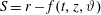 $S=r-f(t,z,\unicode[STIX]{x1D717})$
is characterized by the unit normal vector
$S=r-f(t,z,\unicode[STIX]{x1D717})$
is characterized by the unit normal vector
 $\boldsymbol{n}=\unicode[STIX]{x1D735}S/|\unicode[STIX]{x1D735}S|$
and the interfacial curvature, which simplifies to
$\boldsymbol{n}=\unicode[STIX]{x1D735}S/|\unicode[STIX]{x1D735}S|$
and the interfacial curvature, which simplifies to
 $\unicode[STIX]{x1D735}\boldsymbol{\cdot }\boldsymbol{n}\simeq r^{-1}-f_{zz}-r^{-2}f_{\unicode[STIX]{x1D717}\unicode[STIX]{x1D717}}$
for small departures from a circular cylinder shape. The cylinder is accelerated in the
$\unicode[STIX]{x1D735}\boldsymbol{\cdot }\boldsymbol{n}\simeq r^{-1}-f_{zz}-r^{-2}f_{\unicode[STIX]{x1D717}\unicode[STIX]{x1D717}}$
for small departures from a circular cylinder shape. The cylinder is accelerated in the
 $y$
-direction with a magnitude
$y$
-direction with a magnitude
 $g=|\boldsymbol{g}|$
. Following the classical treatment (Drazin & Reid Reference Drazin and Reid2004), we perform analysis in dimensional variables, except for the numerical results to be presented in § 3.1, which for convenience are in a non-dimensional form.
$g=|\boldsymbol{g}|$
. Following the classical treatment (Drazin & Reid Reference Drazin and Reid2004), we perform analysis in dimensional variables, except for the numerical results to be presented in § 3.1, which for convenience are in a non-dimensional form.

Figure 1. On stability of a cylindrical blob: (a) problem set-up, (b,c) qualitative velocity fields of the base state without (b) and with (c) the lateral acceleration
 $\boldsymbol{g}$
. The vector lengths show the relative velocity magnitudes.
$\boldsymbol{g}$
. The vector lengths show the relative velocity magnitudes.
2.1 Base state
We will study stability of the axisymmetric uniform (i.e. with pure radial growth) cylinder base state, which does not depend on the
 $z$
and
$z$
and
 $\unicode[STIX]{x1D717}$
coordinates:
$\unicode[STIX]{x1D717}$
coordinates:
 $\unicode[STIX]{x1D719}=\unicode[STIX]{x1D6F7}(t,r)$
,
$\unicode[STIX]{x1D719}=\unicode[STIX]{x1D6F7}(t,r)$
,
 $p=P(t,r)$
,
$p=P(t,r)$
,
 $f=F(t)$
. It is straightforward to show from the structure of equations (2.1) that this is possible only if there is no flow in the
$f=F(t)$
. It is straightforward to show from the structure of equations (2.1) that this is possible only if there is no flow in the
 $z$
-direction and
$z$
-direction and
 $g=0$
. Since we are going to consider the case
$g=0$
. Since we are going to consider the case
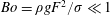 $Bo=\unicode[STIX]{x1D70C}gF^{2}/\unicode[STIX]{x1D70E}\ll 1$
, then deviation from this base state due to acceleration can be treated as a perturbation (§ 4.1). The Laplace equation (2.1a
) admits a non-trivial solution of the above type only when there is a line source at the axis of symmetry providing a mass flux
$Bo=\unicode[STIX]{x1D70C}gF^{2}/\unicode[STIX]{x1D70E}\ll 1$
, then deviation from this base state due to acceleration can be treated as a perturbation (§ 4.1). The Laplace equation (2.1a
) admits a non-trivial solution of the above type only when there is a line source at the axis of symmetry providing a mass flux
 $Q$
, treated here as constant,
$Q$
, treated here as constant,
 $$\begin{eqnarray}\unicode[STIX]{x1D6F7}(t,r)=(Q/2\unicode[STIX]{x03C0})\ln r,\end{eqnarray}$$
producing an axisymmetric flow field; cf. figure 1(b). The logarithmic singularity can be removed by considering a mass source on the cylinder axis of a small radius
 $\unicode[STIX]{x1D716}>0$
. The time-dependent cylinder radius
$\unicode[STIX]{x1D716}>0$
. The time-dependent cylinder radius
 $F(t)$
is found from the kinematic boundary condition (2.1c
), yielding
$F(t)$
is found from the kinematic boundary condition (2.1c
), yielding
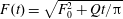 $F(t)=\sqrt{F_{0}^{2}+Qt/\unicode[STIX]{x03C0}}$
, the same as the rim growth on a retracting soap film in the Taylor–Culick theory (Taylor Reference Taylor1959; Culick Reference Culick1960). We will focus, without loss of generality, on the asymptotic case,
$F(t)=\sqrt{F_{0}^{2}+Qt/\unicode[STIX]{x03C0}}$
, the same as the rim growth on a retracting soap film in the Taylor–Culick theory (Taylor Reference Taylor1959; Culick Reference Culick1960). We will focus, without loss of generality, on the asymptotic case,
 $$\begin{eqnarray}F(t)\simeq \sqrt{Qt/\unicode[STIX]{x03C0}},\quad \text{valid for}~t\gg \unicode[STIX]{x03C0}F_{0}^{2}/Q\equiv t_{c}.\end{eqnarray}$$
For a shrinking cylinder, i.e. when
 $t^{\prime }=t_{c}-t\ll t_{c}$
,
$t^{\prime }=t_{c}-t\ll t_{c}$
,
 $F(t)\simeq \sqrt{Qt^{\prime }/\unicode[STIX]{x03C0}}$
, and since
$F(t)\simeq \sqrt{Qt^{\prime }/\unicode[STIX]{x03C0}}$
, and since
 $\unicode[STIX]{x2202}_{t}\rightarrow -\unicode[STIX]{x2202}_{t^{\prime }}$
, the stability results would be the exact opposite of the case considered below. The base state pressure is
$\unicode[STIX]{x2202}_{t}\rightarrow -\unicode[STIX]{x2202}_{t^{\prime }}$
, the stability results would be the exact opposite of the case considered below. The base state pressure is
 $P(t,r)=p_{\infty }+\unicode[STIX]{x1D70E}\unicode[STIX]{x1D735}\boldsymbol{\cdot }\boldsymbol{n}=p_{\infty }+\unicode[STIX]{x1D70E}/r$
, so that the constant
$P(t,r)=p_{\infty }+\unicode[STIX]{x1D70E}\unicode[STIX]{x1D735}\boldsymbol{\cdot }\boldsymbol{n}=p_{\infty }+\unicode[STIX]{x1D70E}/r$
, so that the constant
 $C(t)$
determined by evaluating the Cauchy–Lagrange integral (2.1b
) at the cylinder surface
$C(t)$
determined by evaluating the Cauchy–Lagrange integral (2.1b
) at the cylinder surface
 $r=F(t)$
becomes
$r=F(t)$
becomes
 $C(t)=\unicode[STIX]{x1D70E}/\unicode[STIX]{x1D70C}F(t)+(Q/2\unicode[STIX]{x03C0}F)^{2}/2$
. Then, deviations from this base state due to instability development and lateral acceleration can be treated as perturbations in §§ 3 and 4, respectively.
$C(t)=\unicode[STIX]{x1D70E}/\unicode[STIX]{x1D70C}F(t)+(Q/2\unicode[STIX]{x03C0}F)^{2}/2$
. Then, deviations from this base state due to instability development and lateral acceleration can be treated as perturbations in §§ 3 and 4, respectively.
2.2 Perturbation equation
In the analysis to follow, first, we are going to superimpose general perturbations of the form
 $f(t,z)=F(t)+f^{\prime }(t,\unicode[STIX]{x1D717},z)$
,
$f(t,z)=F(t)+f^{\prime }(t,\unicode[STIX]{x1D717},z)$
,
 $\unicode[STIX]{x1D719}(t,r)=\unicode[STIX]{x1D6F7}(t,r)+\unicode[STIX]{x1D719}^{\prime }(t,\unicode[STIX]{x1D717},r)$
,
$\unicode[STIX]{x1D719}(t,r)=\unicode[STIX]{x1D6F7}(t,r)+\unicode[STIX]{x1D719}^{\prime }(t,\unicode[STIX]{x1D717},r)$
,
 $p(t,r,\unicode[STIX]{x1D717})=P(t,r)+p^{\prime }(t,r,\unicode[STIX]{x1D717})$
. Due to the linearity of inviscid incompressible potential flows, the perturbation of the velocity potential
$p(t,r,\unicode[STIX]{x1D717})=P(t,r)+p^{\prime }(t,r,\unicode[STIX]{x1D717})$
. Due to the linearity of inviscid incompressible potential flows, the perturbation of the velocity potential
 $\unicode[STIX]{x1D719}^{\prime }$
obeys the Laplace equation (2.1a
) as well. Following the same procedure as in the classical case (Drazin & Reid Reference Drazin and Reid2004), modulo the time-dependent boundary
$\unicode[STIX]{x1D719}^{\prime }$
obeys the Laplace equation (2.1a
) as well. Following the same procedure as in the classical case (Drazin & Reid Reference Drazin and Reid2004), modulo the time-dependent boundary
 $r=F(t)$
, the linearization of the kinematic condition (2.1c
), after projecting onto the undisturbed interface
$r=F(t)$
, the linearization of the kinematic condition (2.1c
), after projecting onto the undisturbed interface
 $r=F(t)$
and taking into account that
$r=F(t)$
and taking into account that
 $\unicode[STIX]{x1D6F7}_{r}|_{r=F+f^{\prime }}=\unicode[STIX]{x1D6F7}_{r}|_{F}+\unicode[STIX]{x1D6F7}_{rr}|_{F}\,f^{\prime }\,+\,$
higher-order terms, furnishes
$\unicode[STIX]{x1D6F7}_{r}|_{r=F+f^{\prime }}=\unicode[STIX]{x1D6F7}_{r}|_{F}+\unicode[STIX]{x1D6F7}_{rr}|_{F}\,f^{\prime }\,+\,$
higher-order terms, furnishes
 $$\begin{eqnarray}r=F(t):\frac{\unicode[STIX]{x2202}f^{\prime }}{\unicode[STIX]{x2202}t}=\left.\frac{\unicode[STIX]{x2202}^{2}\unicode[STIX]{x1D6F7}}{\unicode[STIX]{x2202}r^{2}}\right|_{F}f^{\prime }+\frac{\unicode[STIX]{x2202}\unicode[STIX]{x1D719}^{\prime }}{\unicode[STIX]{x2202}r}.\end{eqnarray}$$
Similarly, we can linearize the dynamic condition (2.1b
) around
 $r=F(t)$
,
$r=F(t)$
,
 $$\begin{eqnarray}\frac{\unicode[STIX]{x2202}\unicode[STIX]{x1D719}^{\prime }}{\unicode[STIX]{x2202}t}+\frac{\unicode[STIX]{x2202}\unicode[STIX]{x1D6F7}}{\unicode[STIX]{x2202}r}\left(\frac{\unicode[STIX]{x2202}^{2}\unicode[STIX]{x1D6F7}}{\unicode[STIX]{x2202}r^{2}}f^{\prime }+\frac{\unicode[STIX]{x2202}\unicode[STIX]{x1D719}^{\prime }}{\unicode[STIX]{x2202}r}\right)=-\frac{1}{\unicode[STIX]{x1D70C}}[p|_{r=F+f^{\prime }}-P|_{r=F}]+g\cos \unicode[STIX]{x1D717}(F(t)+f^{\prime }),\end{eqnarray}$$
where the expression in square brackets simplifies given the pressure perturbation at the interface
 $p^{\prime }=-\unicode[STIX]{x1D70E}(f_{zz}+f_{\unicode[STIX]{x1D717}\unicode[STIX]{x1D717}}/F^{2}(t))$
related to the perturbed part of the interfacial curvature
$p^{\prime }=-\unicode[STIX]{x1D70E}(f_{zz}+f_{\unicode[STIX]{x1D717}\unicode[STIX]{x1D717}}/F^{2}(t))$
related to the perturbed part of the interfacial curvature
 $\unicode[STIX]{x1D735}\boldsymbol{\cdot }\boldsymbol{n}$
,
$\unicode[STIX]{x1D735}\boldsymbol{\cdot }\boldsymbol{n}$
,
 $$\begin{eqnarray}[\cdots ]=\left[\left.\frac{\unicode[STIX]{x2202}P}{\unicode[STIX]{x2202}r}\right|_{r=F}f^{\prime }+p^{\prime }\right]=-\left.\frac{\unicode[STIX]{x1D70E}}{r^{2}}\right|_{r=F}f^{\prime }+p^{\prime }=-\unicode[STIX]{x1D70E}\left(\frac{f^{\prime }+\unicode[STIX]{x2202}^{2}f^{\prime }/\unicode[STIX]{x2202}\unicode[STIX]{x1D717}^{2}}{F^{2}(t)}+\frac{\unicode[STIX]{x2202}^{2}f^{\prime }}{\unicode[STIX]{x2202}z^{2}}\right).\end{eqnarray}$$
It should be noted that when calculating
 $\unicode[STIX]{x2202}\unicode[STIX]{x1D6F7}/\unicode[STIX]{x2202}t$
in (2.1b
), we first differentiate (with respect to time
$\unicode[STIX]{x2202}\unicode[STIX]{x1D6F7}/\unicode[STIX]{x2202}t$
in (2.1b
), we first differentiate (with respect to time
 $t$
) and then evaluate at
$t$
) and then evaluate at
 $r=F(t)$
, not vice versa – these two operations do not commute. The same result (2.5) can be arrived at directly from Euler’s equations of fluid motion.
$r=F(t)$
, not vice versa – these two operations do not commute. The same result (2.5) can be arrived at directly from Euler’s equations of fluid motion.
Taking an infinite Fourier transform in the
 $z$
-direction and a finite Fourier transform in the
$z$
-direction and a finite Fourier transform in the
 $\unicode[STIX]{x1D717}$
-direction, the Laplace equation (2.1a
) reduces to
$\unicode[STIX]{x1D717}$
-direction, the Laplace equation (2.1a
) reduces to
 $r^{-1}\unicode[STIX]{x2202}_{r}(r\widehat{\unicode[STIX]{x1D719}}_{r}^{\prime })-(k^{2}+n^{2}/r^{2})\widehat{\unicode[STIX]{x1D719}}^{\prime }=0$
, with the solution expressed in terms of the modified Bessel functions
$r^{-1}\unicode[STIX]{x2202}_{r}(r\widehat{\unicode[STIX]{x1D719}}_{r}^{\prime })-(k^{2}+n^{2}/r^{2})\widehat{\unicode[STIX]{x1D719}}^{\prime }=0$
, with the solution expressed in terms of the modified Bessel functions
 $\widehat{\unicode[STIX]{x1D719}}_{n}^{\prime }=C_{n}I_{n}(kr)+D_{n}K_{n}(kr)$
, where
$\widehat{\unicode[STIX]{x1D719}}_{n}^{\prime }=C_{n}I_{n}(kr)+D_{n}K_{n}(kr)$
, where
 $k$
and
$k$
and
 $n$
are continuous axial and discrete (i.e. quantized due to boundedness of the
$n$
are continuous axial and discrete (i.e. quantized due to boundedness of the
 $\unicode[STIX]{x1D717}$
domain) azimuthal wavenumbers, respectively. Thereby, the conditions (2.4) and (2.5) become
$\unicode[STIX]{x1D717}$
domain) azimuthal wavenumbers, respectively. Thereby, the conditions (2.4) and (2.5) become
 $$\begin{eqnarray}\displaystyle r & = & \displaystyle F(t):\frac{\unicode[STIX]{x2202}}{\unicode[STIX]{x2202}t}\left(\begin{array}{@{}c@{}}\widehat{f}_{n}^{\prime }\\ \widehat{\unicode[STIX]{x1D719}}_{n}^{\prime }\end{array}\right)=\left(\begin{array}{@{}cc@{}}\unicode[STIX]{x1D6F7}_{rr} & \displaystyle \frac{\unicode[STIX]{x2202}}{\unicode[STIX]{x2202}r}\\ \displaystyle -\unicode[STIX]{x1D6F7}_{r}\unicode[STIX]{x1D6F7}_{rr}+\frac{\unicode[STIX]{x1D70E}}{\unicode[STIX]{x1D70C}}\left(\frac{1-n^{2}}{F^{2}(t)}-k^{2}\right) & \displaystyle -\unicode[STIX]{x1D6F7}_{r}\frac{\unicode[STIX]{x2202}}{\unicode[STIX]{x2202}r}\end{array}\right)\left(\begin{array}{@{}c@{}}\widehat{f}_{n}^{\prime }\\ \widehat{\unicode[STIX]{x1D719}}_{n}^{\prime }\end{array}\right)\nonumber\\ \displaystyle & & \displaystyle +\,\frac{g}{2}\left(\begin{array}{@{}c@{}}0\\ \widehat{f}_{n-1}^{\prime }+\widehat{f}_{n+1}^{\prime }\end{array}\right)+\frac{gF}{2}\left(\begin{array}{@{}c@{}}0\\ \unicode[STIX]{x1D6FF}_{n,-1}+\unicode[STIX]{x1D6FF}_{n,1}\end{array}\right),\end{eqnarray}$$
where
 $\unicode[STIX]{x1D6FF}_{n,m}$
is the Kronecker delta function. As we can see from the above system, the base state is affected by acceleration
$\unicode[STIX]{x1D6FF}_{n,m}$
is the Kronecker delta function. As we can see from the above system, the base state is affected by acceleration
 $g$
only at the mode
$g$
only at the mode
 $n=1$
. Moreover, since the system (2.7) is symmetric with respect to the transformation
$n=1$
. Moreover, since the system (2.7) is symmetric with respect to the transformation
 $n\rightarrow -n$
, in the subsequent stability analysis we can focus on
$n\rightarrow -n$
, in the subsequent stability analysis we can focus on
 $n\geqslant 0$
. The system (2.7) is universal in the sense that it allows us to compute both distortion of the base state from a circular cylinder state and the time-dependent perturbation responsible for instability (or stability); in the former case, the amplitude of the distortion is limited by the magnitude
$n\geqslant 0$
. The system (2.7) is universal in the sense that it allows us to compute both distortion of the base state from a circular cylinder state and the time-dependent perturbation responsible for instability (or stability); in the former case, the amplitude of the distortion is limited by the magnitude
 $g$
of acceleration, while in the latter case, the amplitude can grow unboundedly.
$g$
of acceleration, while in the latter case, the amplitude can grow unboundedly.
Modes corresponding to the modified Bessel functions of the first kind
 $I_{n}$
play the dominant role in the instability, since the
$I_{n}$
play the dominant role in the instability, since the
 $K_{n}$
are singular at
$K_{n}$
are singular at
 $r=0$
and decay towards the cylinder surface, where the instability is driven by the surface tension forces. Hence, we can put
$r=0$
and decay towards the cylinder surface, where the instability is driven by the surface tension forces. Hence, we can put
 $D_{n}=0$
as in the classical case of a time-independent cylinder (Drazin & Reid Reference Drazin and Reid2004). If the line source is substituted (to remove the singularity at
$D_{n}=0$
as in the classical case of a time-independent cylinder (Drazin & Reid Reference Drazin and Reid2004). If the line source is substituted (to remove the singularity at
 $r=0$
) by a finite-size mass source
$r=0$
) by a finite-size mass source
 $r\leqslant \unicode[STIX]{x1D716}$
, then the
$r\leqslant \unicode[STIX]{x1D716}$
, then the
 $K_{n}$
would need to be taken into account, but for
$K_{n}$
would need to be taken into account, but for
 $\unicode[STIX]{x1D716}\ll 1$
their contribution should be negligible for the above reasons. With these considerations, we can reduce the system (2.7) to a single second-order equation. From the first equation of (2.7), we determine
$\unicode[STIX]{x1D716}\ll 1$
their contribution should be negligible for the above reasons. With these considerations, we can reduce the system (2.7) to a single second-order equation. From the first equation of (2.7), we determine
 $C_{n}=[\text{d}\widehat{f}_{n}^{\prime }/\text{d}t-\unicode[STIX]{x1D6F7}_{rr}(F)\widehat{f}_{n}^{\prime }]/kI_{n}^{\prime }(kF)$
, where we divided by
$C_{n}=[\text{d}\widehat{f}_{n}^{\prime }/\text{d}t-\unicode[STIX]{x1D6F7}_{rr}(F)\widehat{f}_{n}^{\prime }]/kI_{n}^{\prime }(kF)$
, where we divided by
 $I_{n}^{\prime }(kF)$
since it does not have zeros for
$I_{n}^{\prime }(kF)$
since it does not have zeros for
 $kF\geqslant 0$
, and substituting into the second of equations (2.7) we arrive at a second-order equation for
$kF\geqslant 0$
, and substituting into the second of equations (2.7) we arrive at a second-order equation for
 $\widehat{f}_{n}^{\prime }$
,
$\widehat{f}_{n}^{\prime }$
,
 $$\begin{eqnarray}L\,\widehat{f}_{n}^{\prime }=\frac{\text{d}^{2}\widehat{f}_{n}^{\prime }}{\text{d}t^{2}}+a(t)\frac{\text{d}\widehat{f}_{n}^{\prime }}{\text{d}t}+b(t)\widehat{f}_{n}^{\prime }=\frac{g}{2}(\widehat{f}_{n-1}^{\prime }+\widehat{f}_{n+1}^{\prime })+\frac{gF}{2}(\unicode[STIX]{x1D6FF}_{n,-1}+\unicode[STIX]{x1D6FF}_{n,1}),\end{eqnarray}$$
with the coefficients defined by
 $$\begin{eqnarray}\displaystyle & \displaystyle a(t)=-\unicode[STIX]{x1D6F7}_{rr}(F)-k\frac{I_{n}^{\prime \prime }(kF)}{I_{n}^{\prime }(kF)}\frac{\text{d}F}{\text{d}t}+k\frac{I_{n}^{\prime }(kF)}{I_{n}(kF)}\unicode[STIX]{x1D6F7}_{r}(F), & \displaystyle\end{eqnarray}$$
 $$\begin{eqnarray}\displaystyle & \displaystyle b(t)=-\unicode[STIX]{x1D6F7}_{rrr}(F)\frac{\text{d}F}{\text{d}t}+k\frac{I_{n}^{\prime \prime }(kF)}{I_{n}^{\prime }(kF)}\frac{\text{d}F}{\text{d}t}\unicode[STIX]{x1D6F7}_{rr}(F)-k\frac{I_{n}^{\prime }(kF)}{I_{n}(kF)}\frac{\unicode[STIX]{x1D70E}}{\unicode[STIX]{x1D70C}}\left(\frac{1-n^{2}}{F^{2}}-k^{2}\right). & \displaystyle\end{eqnarray}$$
3 Stability analysis for
 $g=0$
$g=0$

3.1 Numerical integration of the evolution equation
In order to get an initial insight into the solution of (2.8), let us non-dimensionalize it for the convenience of numerical integration only. Letting
 $t=t_{0}\widetilde{t}$
with
$t=t_{0}\widetilde{t}$
with
 $t_{0}=\sqrt{\unicode[STIX]{x1D70C}F_{0}^{3}/\unicode[STIX]{x1D70E}}$
(surface-tension-driven breakup time for a cylinder of radius
$t_{0}=\sqrt{\unicode[STIX]{x1D70C}F_{0}^{3}/\unicode[STIX]{x1D70E}}$
(surface-tension-driven breakup time for a cylinder of radius
 $F_{0}$
), (2.8) reduces to
$F_{0}$
), (2.8) reduces to
 $$\begin{eqnarray}\displaystyle & \displaystyle \frac{\text{d}^{2}\widehat{f}_{n}^{\prime }}{\text{d}\widetilde{t}^{2}}+\widetilde{a}(\widetilde{t})\frac{\text{d}\widehat{f}_{n}^{\prime }}{\text{d}\widetilde{t}}+\widetilde{b}(\widetilde{t})\widehat{f}_{n}^{\prime }=0, & \displaystyle\end{eqnarray}$$
where
 $$\begin{eqnarray}\widetilde{a}(\widetilde{t})=\frac{\widehat{a}(\unicode[STIX]{x1D705})}{2\widetilde{t}},\quad \widetilde{b}(\widetilde{t})=-\frac{1}{4\widetilde{t}^{2}}[2+\widehat{b}_{2}(\unicode[STIX]{x1D705})]-\widehat{b}_{1}(\unicode[STIX]{x1D705})\left(\frac{t_{\ast }}{t_{0}}\right)^{3/2}\frac{1-n^{2}-\unicode[STIX]{x1D705}^{2}}{\widetilde{t}^{3/2}},\end{eqnarray}$$
with the abbreviations
 $\widehat{b}_{1}(\unicode[STIX]{x1D705})=\unicode[STIX]{x1D705}I_{n}^{\prime \prime }(\unicode[STIX]{x1D705})/I_{n}^{\prime }(\unicode[STIX]{x1D705})$
,
$\widehat{b}_{1}(\unicode[STIX]{x1D705})=\unicode[STIX]{x1D705}I_{n}^{\prime \prime }(\unicode[STIX]{x1D705})/I_{n}^{\prime }(\unicode[STIX]{x1D705})$
,
 $\widehat{b}_{2}(\unicode[STIX]{x1D705})=\unicode[STIX]{x1D705}I_{n}^{\prime }(\unicode[STIX]{x1D705})/I_{n}(\widehat{k})$
,
$\widehat{b}_{2}(\unicode[STIX]{x1D705})=\unicode[STIX]{x1D705}I_{n}^{\prime }(\unicode[STIX]{x1D705})/I_{n}(\widehat{k})$
,
 $\widehat{a}(\unicode[STIX]{x1D705})=1+\widehat{b}_{2}(\unicode[STIX]{x1D705})-\widehat{b}_{1}(\unicode[STIX]{x1D705})$
and the non-dimensional wavenumber
$\widehat{a}(\unicode[STIX]{x1D705})=1+\widehat{b}_{2}(\unicode[STIX]{x1D705})-\widehat{b}_{1}(\unicode[STIX]{x1D705})$
and the non-dimensional wavenumber
 $\unicode[STIX]{x1D705}=\widehat{k}\,\widetilde{t}^{\,1/2}$
. Here,
$\unicode[STIX]{x1D705}=\widehat{k}\,\widetilde{t}^{\,1/2}$
. Here,
 $\widehat{k}=\widetilde{k}(t_{0}/t_{\ast })^{1/2}$
,
$\widehat{k}=\widetilde{k}(t_{0}/t_{\ast })^{1/2}$
,
 $\widetilde{k}=kF_{0}$
and the inertial time scale
$\widetilde{k}=kF_{0}$
and the inertial time scale
 $t_{\ast }=\unicode[STIX]{x03C0}F_{0}^{2}/Q\equiv t_{1}$
(which can be interpreted as the time to grow from
$t_{\ast }=\unicode[STIX]{x03C0}F_{0}^{2}/Q\equiv t_{1}$
(which can be interpreted as the time to grow from
 $F=0$
to
$F=0$
to
 $F_{0}$
). Thus, the solution
$F_{0}$
). Thus, the solution
 $\widehat{f}_{n}^{\prime }$
of (3.1a
) can be treated as a function of
$\widehat{f}_{n}^{\prime }$
of (3.1a
) can be treated as a function of
 $\widetilde{t}$
,
$\widetilde{t}$
,
 $n$
and
$n$
and
 $\widehat{k}$
.
$\widehat{k}$
.

Figure 2. Plots of
 $\widehat{f}_{n}^{\prime }$
at different wavenumbers
$\widehat{f}_{n}^{\prime }$
at different wavenumbers
 $\widehat{k}\in [0,0.1]$
for
$\widehat{k}\in [0,0.1]$
for
 $n=0$
and
$n=0$
and
 $t_{\ast }/t_{0}=1$
: (a) short time interval; (b) longer time interval; (c) ultra-long time interval with ultra-short wavenumbers
$t_{\ast }/t_{0}=1$
: (a) short time interval; (b) longer time interval; (c) ultra-long time interval with ultra-short wavenumbers
 $\widehat{k}=O(10^{-6})$
; (d) solution for
$\widehat{k}=O(10^{-6})$
; (d) solution for
 $\widehat{k}=2\times 10^{-2}$
from figure 2(b) for three values of
$\widehat{k}=2\times 10^{-2}$
from figure 2(b) for three values of
 $t_{\ast }/t_{0}$
.
$t_{\ast }/t_{0}$
.
If one naively applies the stability results for a time-independent cylinder to a time-dependent one, it seems to be intuitive to hypothesize that the most unstable wavenumber should still scale as
 $k\sim F^{-1}$
, now being time-dependent. Indeed, after analysing equations (3.1) with
$k\sim F^{-1}$
, now being time-dependent. Indeed, after analysing equations (3.1) with
 $\unicode[STIX]{x1D705}=\text{const.}$
, we conclude that for large time,
$\unicode[STIX]{x1D705}=\text{const.}$
, we conclude that for large time,
 $\widetilde{t}\rightarrow \infty$
, the solution behaves as
$\widetilde{t}\rightarrow \infty$
, the solution behaves as
 $$\begin{eqnarray}\widehat{f}_{0}^{\prime }\sim \widetilde{t}^{-\widehat{a}(\unicode[STIX]{x1D705})/4-(1/8)}\text{e}^{4\sqrt{c}\,\,\widetilde{t}^{\,1/4}},\quad c=\widehat{b}_{2}(\unicode[STIX]{x1D705})(1-\unicode[STIX]{x1D705}^{2})(t_{\ast }/t_{0})^{3/2}.\end{eqnarray}$$
For truly
 $\widetilde{t}\rightarrow +\infty$
, the growth is dominated by the exponential only, so that the maximum growth rate is achieved when
$\widetilde{t}\rightarrow +\infty$
, the growth is dominated by the exponential only, so that the maximum growth rate is achieved when
 $c(\unicode[STIX]{x1D705})$
is at maximum, which occurs at some finite
$c(\unicode[STIX]{x1D705})$
is at maximum, which occurs at some finite
 $\unicode[STIX]{x1D705}=O(1)$
similar to the classical dispersion relation (3.5); cf. also figure 1.5 of Drazin & Reid (Reference Drazin and Reid2004). For finite times, the optimum
$\unicode[STIX]{x1D705}=O(1)$
similar to the classical dispersion relation (3.5); cf. also figure 1.5 of Drazin & Reid (Reference Drazin and Reid2004). For finite times, the optimum
 $\unicode[STIX]{x1D705}$
is affected by
$\unicode[STIX]{x1D705}$
is affected by
 $a(\unicode[STIX]{x1D705})$
as well. The problem with the above hypothesis
$a(\unicode[STIX]{x1D705})$
as well. The problem with the above hypothesis
 $k\sim F^{-1}$
is that it implicitly requires the Fourier transform with time-dependent wavenumber to commute with the operation of the time derivative, whereas they clearly do not. Hence, it can be surmised that the hypothesis is not viable. In fact, by solving an initial value problem for (3.1a
), we can validate this suspicion. Before that, let us first make a few observations from numerical solution of (3.1), which can be constructed accurately even for long times using the conservative nature of the problem at hand and hence appealing to symplectic integrator methods.
$k\sim F^{-1}$
is that it implicitly requires the Fourier transform with time-dependent wavenumber to commute with the operation of the time derivative, whereas they clearly do not. Hence, it can be surmised that the hypothesis is not viable. In fact, by solving an initial value problem for (3.1a
), we can validate this suspicion. Before that, let us first make a few observations from numerical solution of (3.1), which can be constructed accurately even for long times using the conservative nature of the problem at hand and hence appealing to symplectic integrator methods.
From figure 2(a), the mode entanglement makes it clear that the growth is not monotonic with the wavenumber
 $k$
and time
$k$
and time
 $t$
. Moreover, what appears to be a ‘winning’ mode (bold) on a short time interval becomes a decaying oscillating mode on a longer time interval; cf. figure 2(b). It also appears, cf. figure 2(c), that there is no short-wavenumber cutoff – the limit
$t$
. Moreover, what appears to be a ‘winning’ mode (bold) on a short time interval becomes a decaying oscillating mode on a longer time interval; cf. figure 2(b). It also appears, cf. figure 2(c), that there is no short-wavenumber cutoff – the limit
 $k\rightarrow 0$
indicates that the perturbation starts to grow at a very long time and brings up larger maxima of the solution
$k\rightarrow 0$
indicates that the perturbation starts to grow at a very long time and brings up larger maxima of the solution
 $\widehat{f}_{0}^{\prime }$
compared with shorter wavelengths. The latter observation suggests that there is no optimal, i.e. most amplified, wavenumber, as the maximum achieved increases with decreasing
$\widehat{f}_{0}^{\prime }$
compared with shorter wavelengths. The latter observation suggests that there is no optimal, i.e. most amplified, wavenumber, as the maximum achieved increases with decreasing
 $k$
. Any wavenumber
$k$
. Any wavenumber
 $k$
, no matter how small, is eventually amplified and then damped; cf. figure 2(c). Finally, as observed from figure 2(d), increase of the inertial over the surface tension time scale brings up the decaying oscillation stage closer in time. Overall, figure 2 suggests that there is no single most amplified wavenumber
$k$
, no matter how small, is eventually amplified and then damped; cf. figure 2(c). Finally, as observed from figure 2(d), increase of the inertial over the surface tension time scale brings up the decaying oscillation stage closer in time. Overall, figure 2 suggests that there is no single most amplified wavenumber
 $\widehat{k}$
, and hence the stability should be interpreted in terms different from those in standard eigenvalue studies. The purpose of the subsequent discussion is to disentangle the observed dynamics.
$\widehat{k}$
, and hence the stability should be interpreted in terms different from those in standard eigenvalue studies. The purpose of the subsequent discussion is to disentangle the observed dynamics.
3.2 Long-wave approximation
To get a better sense of the system behaviour, let us consider a long-wave,
 $kF\ll 1$
, and long-time,
$kF\ll 1$
, and long-time,
 $t\gg t_{c}$
, approximation. Introducing
$t\gg t_{c}$
, approximation. Introducing
 $u_{n}=\widehat{f}_{n}^{\prime }\,\text{exp}(\int a\,\text{d}t/2)$
, we can reduce (2.8) to
$u_{n}=\widehat{f}_{n}^{\prime }\,\text{exp}(\int a\,\text{d}t/2)$
, we can reduce (2.8) to
 $$\begin{eqnarray}u_{n}^{\prime \prime }-s^{2}(t)u_{n}=0,\quad \text{where}~s^{2}(t)=-b+{\textstyle \frac{1}{2}}a_{t}+{\textstyle \frac{1}{4}}a^{2}.\end{eqnarray}$$
Depending upon the index
 $n$
of the Bessel function, we obtain
$n$
of the Bessel function, we obtain
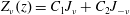
 $$\begin{eqnarray}\displaystyle & \displaystyle n=0:s^{2}(t)=\frac{1}{4t^{2}}+\frac{k^{2}}{2F}\frac{\unicode[STIX]{x1D70E}}{\unicode[STIX]{x1D70C}}(1-k^{2}F^{2})+\frac{1}{4}\left(\frac{Q}{4\unicode[STIX]{x03C0}}k^{2}\right)^{2}, & \displaystyle\end{eqnarray}$$
 $$\begin{eqnarray}\displaystyle & \displaystyle n\neq 0:s^{2}(t)=\frac{n}{4t^{2}}+\frac{n}{F^{3}}\frac{\unicode[STIX]{x1D70E}}{\unicode[STIX]{x1D70C}}(1-n^{2}-k^{2}F^{2}), & \displaystyle\end{eqnarray}$$
 $F=\text{const.}$
,
$F=\text{const.}$
,  $$\begin{eqnarray}s^{2}=\frac{\unicode[STIX]{x1D70E}}{\unicode[STIX]{x1D70C}}\frac{1}{F^{3}}\frac{kFI_{n}^{\prime }(kF)}{I_{n}(kF)}(1-n^{2}-k^{2}F^{2}),\end{eqnarray}$$
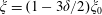
with the asymptotics in the long-wave approximation,
 $$\begin{eqnarray}n=0:s^{2}\simeq \frac{\unicode[STIX]{x1D70E}}{\unicode[STIX]{x1D70C}}\frac{k^{2}}{2F}(1-k^{2}F^{2}),\quad n\neq 0:s^{2}\simeq \frac{\unicode[STIX]{x1D70E}}{\unicode[STIX]{x1D70C}}\frac{n}{F^{3}}(1-n^{2}-k^{2}F^{2}),\end{eqnarray}$$
where now
 $s$
has the meaning of a growth rate (eigenvalue), i.e.
$s$
has the meaning of a growth rate (eigenvalue), i.e.
 $\widehat{f}_{n}^{\prime }\sim \text{e}^{st}$
: for
$\widehat{f}_{n}^{\prime }\sim \text{e}^{st}$
: for
 $n=0$
(axisymmetric mode), the growth is observed for
$n=0$
(axisymmetric mode), the growth is observed for
 $k^{2}F^{2}<1$
, while for
$k^{2}F^{2}<1$
, while for
 $n\geqslant 1$
, all modes are stable (not growing). The dispersion relation (3.6) suggests that the growth rate in the classical case vanishes in the limit of
$n\geqslant 1$
, all modes are stable (not growing). The dispersion relation (3.6) suggests that the growth rate in the classical case vanishes in the limit of
 $k=0$
(long waves, for which the surface tension
$k=0$
(long waves, for which the surface tension
 $\unicode[STIX]{x1D70E}$
is ineffective) and at
$\unicode[STIX]{x1D70E}$
is ineffective) and at
 $k=F^{-1}$
(short waves, when the surface tension starts to suppress instability). Clearly, the long-wave asymptotics is accurate enough to determine the optimal mode
$k=F^{-1}$
(short waves, when the surface tension starts to suppress instability). Clearly, the long-wave asymptotics is accurate enough to determine the optimal mode
 $n$
and wavelength
$n$
and wavelength
 $k$
; indeed, expression (3.6) for
$k$
; indeed, expression (3.6) for
 $n=0$
gives
$n=0$
gives
 $kF=0.707$
, versus the precise 0.697 from (3.5). These results are recovered from the time-dependent case (3.4a
) if one puts
$kF=0.707$
, versus the precise 0.697 from (3.5). These results are recovered from the time-dependent case (3.4a
) if one puts
 $F=\text{const.}$
,
$F=\text{const.}$
,
 $Q=0$
and
$Q=0$
and
 $t\rightarrow \infty$
.
$t\rightarrow \infty$
.
In the time-dependent case, when
 $n=0$
and
$n=0$
and
 $t\rightarrow \infty$
, we observe that for
$t\rightarrow \infty$
, we observe that for
 $k\rightarrow 0$
,
$k\rightarrow 0$
,
 $s^{2}=(k^{2}/2F)(\unicode[STIX]{x1D70E}/\unicode[STIX]{x1D70C})>0$
, i.e. a long-wave instability is expected; for
$s^{2}=(k^{2}/2F)(\unicode[STIX]{x1D70E}/\unicode[STIX]{x1D70C})>0$
, i.e. a long-wave instability is expected; for
 $k\rightarrow \infty$
, the coefficients in (2.8) become
$k\rightarrow \infty$
, the coefficients in (2.8) become
 $$\begin{eqnarray}a(t)=\frac{1}{2t},\quad b(t)=-\frac{1}{2t^{2}}-\frac{k}{4}\frac{Q}{\unicode[STIX]{x03C0}t}\sqrt{\frac{\unicode[STIX]{x03C0}}{Qt}}-\frac{k\unicode[STIX]{x03C0}}{Qt}\frac{\unicode[STIX]{x1D70E}}{\unicode[STIX]{x1D70C}}(1-n^{2}-k^{2}F^{2})\simeq k^{3}\frac{\unicode[STIX]{x1D70E}}{\unicode[STIX]{x1D70C}},\end{eqnarray}$$
so that
 $s^{2}(t)=-k^{3}\unicode[STIX]{x1D70E}/\unicode[STIX]{x1D70C}$
, i.e. the surface tension has a stabilizing effect on short wavelengths in the long-time limit. Based on the above, one might expect that for some large fixed time
$s^{2}(t)=-k^{3}\unicode[STIX]{x1D70E}/\unicode[STIX]{x1D70C}$
, i.e. the surface tension has a stabilizing effect on short wavelengths in the long-time limit. Based on the above, one might expect that for some large fixed time
 $t$
(independent of
$t$
(independent of
 $k$
), there exists a sufficiently large wavenumber
$k$
), there exists a sufficiently large wavenumber
 $k$
at which
$k$
at which
 $s^{2}$
changes sign from positive to negative and hence, loosely speaking, growth is succeeded by decay in time. While general ordinary differential equation theorems (Bellman Reference Bellman1949; Kamke Reference Kamke1961) applied to (3.3) suggest that instability is plausible, they do not provide any insight into the wavenumber structure of the growing/decaying perturbation. Hence, the rest of this section is devoted to a detailed analysis of the instability phenomena.
$s^{2}$
changes sign from positive to negative and hence, loosely speaking, growth is succeeded by decay in time. While general ordinary differential equation theorems (Bellman Reference Bellman1949; Kamke Reference Kamke1961) applied to (3.3) suggest that instability is plausible, they do not provide any insight into the wavenumber structure of the growing/decaying perturbation. Hence, the rest of this section is devoted to a detailed analysis of the instability phenomena.
3.3 Stability time intervals
Instability develops over several distinct time intervals, defined by the values of
 $Q$
,
$Q$
,
 $\unicode[STIX]{x1D70E}/\unicode[STIX]{x1D70C}$
and
$\unicode[STIX]{x1D70E}/\unicode[STIX]{x1D70C}$
and
 $k$
. In the following analysis, we discuss the solution of (3.3) for
$k$
. In the following analysis, we discuss the solution of (3.3) for
 $u_{0}(t)$
, bearing in mind that it is related to the total solution via
$u_{0}(t)$
, bearing in mind that it is related to the total solution via
 $\widehat{f}_{0}^{\prime }(t)=\text{e}^{-t/8t_{1}}u_{0}(t)$
. In the classical case (3.6), the exponential factor is absent as
$\widehat{f}_{0}^{\prime }(t)=\text{e}^{-t/8t_{1}}u_{0}(t)$
. In the classical case (3.6), the exponential factor is absent as
 $t_{1}=\infty$
. In addition to the mass supply time scale
$t_{1}=\infty$
. In addition to the mass supply time scale
 $t_{1}=\unicode[STIX]{x03C0}/Qk^{2}$
previously introduced with
$t_{1}=\unicode[STIX]{x03C0}/Qk^{2}$
previously introduced with
 $k=F_{0}^{-1}$
, the surface tension time scale
$k=F_{0}^{-1}$
, the surface tension time scale
 $t_{2}=(Q/\unicode[STIX]{x03C0})^{3}(\unicode[STIX]{x1D70C}/\unicode[STIX]{x1D70E})^{2}$
emerges. We focus on axisymmetric disturbances,
$t_{2}=(Q/\unicode[STIX]{x03C0})^{3}(\unicode[STIX]{x1D70C}/\unicode[STIX]{x1D70E})^{2}$
emerges. We focus on axisymmetric disturbances,
 $n=0$
, as the most unstable ones in order to analyse the time intervals on which different terms in (3.4a
) dominate.
$n=0$
, as the most unstable ones in order to analyse the time intervals on which different terms in (3.4a
) dominate.
Case 1:
 $((Q/8\unicode[STIX]{x03C0})k^{2})^{2}$
is dominant if
$((Q/8\unicode[STIX]{x03C0})k^{2})^{2}$
is dominant if
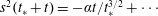
 $$\begin{eqnarray}t\gg 4t_{1}\quad \text{and}\quad t\gg 4^{5}t_{1}^{2}t_{2}^{-1}\quad \text{and}\quad t\ll 4^{-5}t_{2},\end{eqnarray}$$
which is possible provided that
 $t_{2}$
is large enough and
$t_{2}$
is large enough and
 $t_{1}$
is sufficiently small. In this case, we get a linear oscillator equation with the solution
$t_{1}$
is sufficiently small. In this case, we get a linear oscillator equation with the solution
 $$\begin{eqnarray}u_{0}(t)=C_{1}\text{e}^{(Q/8\unicode[STIX]{x03C0})k^{2}t}+C_{2}\text{e}^{-(Q/8\unicode[STIX]{x03C0})k^{2}t};\end{eqnarray}$$
i.e. exponential growth of
 $u_{0}(t)$
is observed, with the most unstable wavenumber being
$u_{0}(t)$
is observed, with the most unstable wavenumber being
 $k=\infty$
(short waves), which is expected as surface tension is not present in this limit; of course, the conditions (3.8) are invalidated then. However,
$k=\infty$
(short waves), which is expected as surface tension is not present in this limit; of course, the conditions (3.8) are invalidated then. However,
 $\widehat{f}_{0}^{\prime }(t)$
(and hence the blob) is not prone to a Rayleigh–Taylor instability; in fact, the acceleration of the interface
$\widehat{f}_{0}^{\prime }(t)$
(and hence the blob) is not prone to a Rayleigh–Taylor instability; in fact, the acceleration of the interface
 $F_{tt}\sim -t^{-3/2}$
is negative at this stage. The observed behaviour in this case corresponds to the flat part of the graphs in figure 2(c). The presence of the term
$F_{tt}\sim -t^{-3/2}$
is negative at this stage. The observed behaviour in this case corresponds to the flat part of the graphs in figure 2(c). The presence of the term
 $(Qk^{2}/4\unicode[STIX]{x03C0})^{2}/4=4^{-3}t_{1}^{-2}$
is due to the radial acceleration of the cylinder interface, as can be gleaned from (2.3).
$(Qk^{2}/4\unicode[STIX]{x03C0})^{2}/4=4^{-3}t_{1}^{-2}$
is due to the radial acceleration of the cylinder interface, as can be gleaned from (2.3).
Case 2:
 $1/4t^{2}$
is dominant if
$1/4t^{2}$
is dominant if
 $$\begin{eqnarray}t\ll 4t_{1}\quad \text{and}\quad t\ll (4^{-1}t_{1}^{2}t_{2})^{1/3}\quad \text{and}\quad t\ll (4^{-1}t_{1}^{4}t_{2})^{1/5},\end{eqnarray}$$
which is possible provided that both
 $t_{1}$
and
$t_{1}$
and
 $t_{2}$
are large enough, i.e. the behaviour corresponds to the earlier time growth in figure 2(a). Since in this case
$t_{2}$
are large enough, i.e. the behaviour corresponds to the earlier time growth in figure 2(a). Since in this case
 $s^{2}(t)=1/(4t^{2})$
, we get Euler’s equation, admitting the solution
$s^{2}(t)=1/(4t^{2})$
, we get Euler’s equation, admitting the solution
 $$\begin{eqnarray}u_{0}(t)=C_{1}t^{(1/2)+(1/\sqrt{2})}+C_{2}t^{(1/2)-(1/\sqrt{2})},\end{eqnarray}$$
i.e. algebraic growth is observed.
Case 3:
 $(k^{4}/2)(\unicode[STIX]{x1D70E}/\unicode[STIX]{x1D70C})F$
is dominant if
$(k^{4}/2)(\unicode[STIX]{x1D70E}/\unicode[STIX]{x1D70C})F$
is dominant if
 $$\begin{eqnarray}t\gg t_{1}\quad \text{and}\quad t\gg 4^{-5}t_{2}\quad \text{and}\quad t\gg (4^{-1}t_{1}^{4}t_{2})^{1/5},\end{eqnarray}$$
which is possible provided that both
 $t_{1}$
and
$t_{1}$
and
 $t_{2}$
are small enough. In this case, the solution can be expressed in terms of Bessel functions of fractional order
$t_{2}$
are small enough. In this case, the solution can be expressed in terms of Bessel functions of fractional order
 $\unicode[STIX]{x1D708}$
, namely
$\unicode[STIX]{x1D708}$
, namely
 $$\begin{eqnarray}u_{0}(t)=\sqrt{t}Z_{1/2q}\left(\frac{\text{i}}{q}\sqrt{c}t^{q}\right),\quad \text{where}~\frac{1}{2q}=\frac{2}{5},\,c=-\frac{k^{4}}{2}\frac{\unicode[STIX]{x1D70E}}{\unicode[STIX]{x1D70C}}\sqrt{\frac{Q}{\unicode[STIX]{x03C0}}},\end{eqnarray}$$
and
 $Z_{\unicode[STIX]{x1D708}}(z)=C_{1}J_{\unicode[STIX]{x1D708}}+C_{2}J_{-\unicode[STIX]{x1D708}}$
, with the asymptotics for large
$Z_{\unicode[STIX]{x1D708}}(z)=C_{1}J_{\unicode[STIX]{x1D708}}+C_{2}J_{-\unicode[STIX]{x1D708}}$
, with the asymptotics for large
 $z$
(large time
$z$
(large time
 $t$
),
$t$
),
 $$\begin{eqnarray}J_{\unicode[STIX]{x1D708}}(z)=\sqrt{2/\unicode[STIX]{x1D708}z}\cos [z-(2\unicode[STIX]{x1D708}+1)\unicode[STIX]{x03C0}/4]+O(z^{-3/2})\quad \text{as}~z\rightarrow \infty .\end{eqnarray}$$
Hence,
 $u_{0}(t)\sim t^{-1/8}\cos (\unicode[STIX]{x1D6FC}t^{5/4})+\cdots \rightarrow 0$
as
$u_{0}(t)\sim t^{-1/8}\cos (\unicode[STIX]{x1D6FC}t^{5/4})+\cdots \rightarrow 0$
as
 $t\rightarrow +\infty$
.
$t\rightarrow +\infty$
.
Case 4:
 $(k^{2}/2F)(\unicode[STIX]{x1D70E}/\unicode[STIX]{x1D70C})$
is dominant if
$(k^{2}/2F)(\unicode[STIX]{x1D70E}/\unicode[STIX]{x1D70C})$
is dominant if
 $$\begin{eqnarray}t\ll t_{1}\quad \text{and}\quad t\ll 4^{5}t_{1}^{2}t_{2}^{-1}\quad \text{and}\quad t\gg (4^{-1}t_{1}^{2}t_{2})^{1/3},\end{eqnarray}$$
which is possible provided that
 $t_{1}$
is large enough and
$t_{1}$
is large enough and
 $t_{2}$
is sufficiently small. In this case,
$t_{2}$
is sufficiently small. In this case,
 $s^{2}(t)=ct^{-1/2}$
, with
$s^{2}(t)=ct^{-1/2}$
, with
 $c=2^{-1}t_{1}^{-1}t_{2}^{-1/2}$
, and thus
$c=2^{-1}t_{1}^{-1}t_{2}^{-1/2}$
, and thus
 $$\begin{eqnarray}u_{0}=t^{1/2}Z_{1/3}\left({\textstyle \frac{4}{3}}\text{i}c^{1/2}t^{3/4}\right),\end{eqnarray}$$
where
 $Z_{\unicode[STIX]{x1D708}}(z)=C_{1}J_{\unicode[STIX]{x1D708}}(z)+C_{2}J_{-\unicode[STIX]{x1D708}}(z)$
,
$Z_{\unicode[STIX]{x1D708}}(z)=C_{1}J_{\unicode[STIX]{x1D708}}(z)+C_{2}J_{-\unicode[STIX]{x1D708}}(z)$
,
 $z=\text{i}\unicode[STIX]{x1D6FC}t^{3/4}$
and
$z=\text{i}\unicode[STIX]{x1D6FC}t^{3/4}$
and
 $\unicode[STIX]{x1D6FC}=(4/3)c^{1/2}$
, with the asymptotics
$\unicode[STIX]{x1D6FC}=(4/3)c^{1/2}$
, with the asymptotics
 $u_{0}(t)\sim t^{-3/8}\text{e}^{\unicode[STIX]{x1D6FC}t^{3/4}}$
. Hence, the solution first grows (case 4) and then decays in an oscillating fashion (case 3) in time, as observed in figures 2(a–c). Thus, the combination of cases 3 and 4 is analogous to the classical situation (3.6), and therefore one then might infer that selection of the most amplified wavenumber
$u_{0}(t)\sim t^{-3/8}\text{e}^{\unicode[STIX]{x1D6FC}t^{3/4}}$
. Hence, the solution first grows (case 4) and then decays in an oscillating fashion (case 3) in time, as observed in figures 2(a–c). Thus, the combination of cases 3 and 4 is analogous to the classical situation (3.6), and therefore one then might infer that selection of the most amplified wavenumber
 $k$
should be made possible when two terms –
$k$
should be made possible when two terms –
 $(k^{2}/2F)(\unicode[STIX]{x1D70E}/\unicode[STIX]{x1D70C})$
and
$(k^{2}/2F)(\unicode[STIX]{x1D70E}/\unicode[STIX]{x1D70C})$
and
 $(k^{4}/2)(\unicode[STIX]{x1D70E}/\unicode[STIX]{x1D70C})F$
– compete, similarly to the classical Rayleigh–Plateau instability. However, this expectation proves to be unfeasible.
$(k^{4}/2)(\unicode[STIX]{x1D70E}/\unicode[STIX]{x1D70C})F$
– compete, similarly to the classical Rayleigh–Plateau instability. However, this expectation proves to be unfeasible.
3.4 On non-existence of optimal growth time and wavenumber
Here, we will consider cases 3 and 4 together (omitting index 0), which leads to the equation
 $$\begin{eqnarray}u^{\prime \prime }-s^{2}(t)u=0,\quad s^{2}(t)=\frac{\unicode[STIX]{x1D6FC}}{\sqrt{t}}-\unicode[STIX]{x1D6FD}\sqrt{t},\quad \text{with}~\unicode[STIX]{x1D6FC}=\frac{k^{2}}{2}\frac{\unicode[STIX]{x1D70E}}{\unicode[STIX]{x1D70C}}\sqrt{\frac{\unicode[STIX]{x03C0}}{Q}},\,\unicode[STIX]{x1D6FD}=\unicode[STIX]{x1D6FC}\frac{k^{2}Q}{\unicode[STIX]{x03C0}}.\end{eqnarray}$$
The sign of
 $s^{2}(t)$
changes at the ‘turning’ point
$s^{2}(t)$
changes at the ‘turning’ point
 $t_{\ast }$
, which coincidentally equals the previously introduced inertial time scale
$t_{\ast }$
, which coincidentally equals the previously introduced inertial time scale
 $t_{\ast }=\unicode[STIX]{x1D6FC}/\unicode[STIX]{x1D6FD}\equiv t_{1}$
. The solution to this problem is amenable to the Wentzel–Kramers–Brillouin method, namely away from the turning point it renders
$t_{\ast }=\unicode[STIX]{x1D6FC}/\unicode[STIX]{x1D6FD}\equiv t_{1}$
. The solution to this problem is amenable to the Wentzel–Kramers–Brillouin method, namely away from the turning point it renders
 $$\begin{eqnarray}u(t)=\frac{C_{\pm }}{[s^{2}(t)]^{1/4}}\exp \left[\pm \int _{t_{0}}^{t}\sqrt{s^{2}(\unicode[STIX]{x1D70F})}\,\text{d}\unicode[STIX]{x1D70F}\right],\end{eqnarray}$$
which after Taylor expansion of
 $s^{2}(t)$
near
$s^{2}(t)$
near
 $t_{\ast }$
,
$t_{\ast }$
,
 $s^{2}(t_{\ast }+t)=-\unicode[STIX]{x1D6FC}t/t_{\ast }^{3/2}+\cdots$
, with
$s^{2}(t_{\ast }+t)=-\unicode[STIX]{x1D6FC}t/t_{\ast }^{3/2}+\cdots$
, with
 $t$
now measured from the turning point
$t$
now measured from the turning point
 $t_{\ast }$
, becomes
$t_{\ast }$
, becomes
 $$\begin{eqnarray}\displaystyle & \displaystyle t>0:u=\frac{t_{\ast }^{3/8}}{(\unicode[STIX]{x1D6FC}t)^{1/4}}[A\text{e}^{\text{i}(2/3)(\unicode[STIX]{x1D6FC}^{1/2}/t_{\ast }^{3/4})t^{3/2}}+B\text{e}^{-\text{i}(2/3)(\unicode[STIX]{x1D6FC}^{1/2}/t_{\ast }^{3/4})t^{3/2}}], & \displaystyle\end{eqnarray}$$
 $$\begin{eqnarray}\displaystyle & \displaystyle t<0:u=\frac{t_{\ast }^{3/8}}{(-\unicode[STIX]{x1D6FC}t)^{1/4}}[C\text{e}^{-(2/3)(\unicode[STIX]{x1D6FC}^{1/2}/t_{\ast }^{3/4})(-t)^{3/2}}+D\text{e}^{(2/3)(\unicode[STIX]{x1D6FC}^{1/2}/t_{\ast }^{3/4})(-t)^{3/2}}], & \displaystyle\end{eqnarray}$$
 $D=0$
, as for
$D=0$
, as for
 $t\rightarrow -\infty$
, the solution should be bounded.
$t\rightarrow -\infty$
, the solution should be bounded.
In a neighbourhood of the turning point, (3.17) simplifies to the Airy equation
 $$\begin{eqnarray}u^{\prime \prime }+\unicode[STIX]{x1D6FC}tt_{\ast }^{-3/2}u=0,\end{eqnarray}$$
the solution of which is expressed in terms of Airy functions
 $u_{0}(t)=a\,\text{Ai}(z)+b\,\text{Bi}(z)$
,
$u_{0}(t)=a\,\text{Ai}(z)+b\,\text{Bi}(z)$
,
 $z=-\unicode[STIX]{x1D6FC}^{1/3}t_{\ast }^{-1/2}t$
. In order to determine the constants
$z=-\unicode[STIX]{x1D6FC}^{1/3}t_{\ast }^{-1/2}t$
. In order to determine the constants
 $a$
and
$a$
and
 $b$
, we will need the asymptotics of
$b$
, we will need the asymptotics of
 $\text{Ai}$
and
$\text{Ai}$
and
 $\text{Bi}$
for
$\text{Bi}$
for
 $z\gg 1(t\rightarrow -\infty )$
and
$z\gg 1(t\rightarrow -\infty )$
and
 $-z\gg 1(t\rightarrow +\infty )$
(Abramowitz & Stegun Reference Abramowitz and Stegun1965). Matching these asymptotics with the Wentzel–Kramers–Brillouin solutions (3.19) for both
$-z\gg 1(t\rightarrow +\infty )$
(Abramowitz & Stegun Reference Abramowitz and Stegun1965). Matching these asymptotics with the Wentzel–Kramers–Brillouin solutions (3.19) for both
 $t\rightarrow \pm \infty$
, we find
$t\rightarrow \pm \infty$
, we find
 $$\begin{eqnarray}A=\frac{\text{e}^{\text{i}(\unicode[STIX]{x03C0}/4)}}{2\sqrt{\unicode[STIX]{x03C0}}}\frac{\unicode[STIX]{x1D6FC}^{1/6}}{t_{\ast }^{1/4}}[b-\text{i}a],\quad B=\frac{\text{e}^{-\text{i}(\unicode[STIX]{x03C0}/4)}}{2\sqrt{\unicode[STIX]{x03C0}}}\frac{\unicode[STIX]{x1D6FC}^{1/6}}{t_{\ast }^{1/4}}[b+\text{i}a],\quad C=\frac{a}{2\sqrt{\unicode[STIX]{x03C0}}}\frac{\unicode[STIX]{x1D6FC}^{1/6}}{t_{\ast }^{1/4}},\quad D=\frac{b}{\sqrt{\unicode[STIX]{x03C0}}}\frac{\unicode[STIX]{x1D6FC}^{1/6}}{t_{\ast }^{1/4}}.\end{eqnarray}$$
Since
 $D=0$
, then
$D=0$
, then
 $b=0$
. As a result, the solution for
$b=0$
. As a result, the solution for
 $t>0$
, i.e. after the turning point
$t>0$
, i.e. after the turning point
 $t_{\ast }$
, reads
$t_{\ast }$
, reads
 $$\begin{eqnarray}u(t)=C\frac{2t_{\ast }^{3/8}}{\unicode[STIX]{x1D6FC}^{1/4}t^{1/4}}\sin \left(\unicode[STIX]{x1D709}+\frac{\unicode[STIX]{x03C0}}{4}\right),\quad \text{where}~\unicode[STIX]{x1D709}=\frac{2}{3}\frac{\unicode[STIX]{x1D6FC}^{1/2}}{t_{\ast }^{3/4}}t^{3/2},\end{eqnarray}$$
and thus the interfacial deflection becomes
 $\widehat{f}^{\prime }(t)=\text{e}^{-1/2\int a\,\text{d}t}u(t)=\text{const.}\,\text{e}^{-t/8t_{\ast }}u(t)$
, where again
$\widehat{f}^{\prime }(t)=\text{e}^{-1/2\int a\,\text{d}t}u(t)=\text{const.}\,\text{e}^{-t/8t_{\ast }}u(t)$
, where again
 $t$
is defined relative to the turning point
$t$
is defined relative to the turning point
 $t_{\ast }$
. To determine the maximum achieved during the time evolution, we differentiate the above (total) solution,
$t_{\ast }$
. To determine the maximum achieved during the time evolution, we differentiate the above (total) solution,
 $$\begin{eqnarray}\frac{\text{d}}{\text{d}t}[\text{e}^{-t/8t_{\ast }}u(t)]=0\Rightarrow \frac{1}{6}\tan \left(\unicode[STIX]{x1D709}+\frac{\unicode[STIX]{x03C0}}{4}\right)[\unicode[STIX]{x1D6FF}\unicode[STIX]{x1D709}^{2/3}+1]=\unicode[STIX]{x1D709},\quad \unicode[STIX]{x1D6FF}=\frac{3^{2/3}}{2^{4/3}}\left(\frac{t_{2}}{t_{1}}\right)^{1/6}\ll 1,\end{eqnarray}$$
where
 $\unicode[STIX]{x1D6FF}\ll 1$
since
$\unicode[STIX]{x1D6FF}\ll 1$
since
 $t_{2}/t_{1}\ll 1$
in the considered case 4. For
$t_{2}/t_{1}\ll 1$
in the considered case 4. For
 $\unicode[STIX]{x1D6FF}=0$
, the above extremum condition admits the approximate solution reflecting the presence of infinitely many ‘humps’ (cf. figure 3),
$\unicode[STIX]{x1D6FF}=0$
, the above extremum condition admits the approximate solution reflecting the presence of infinitely many ‘humps’ (cf. figure 3),
 $$\begin{eqnarray}\unicode[STIX]{x1D709}_{0}=\unicode[STIX]{x03C0}\left(m+\frac{1}{4}\right)-\unicode[STIX]{x1D709}^{\prime },\quad \unicode[STIX]{x1D709}^{\prime }=\frac{2}{3\unicode[STIX]{x03C0}}\frac{1}{1+4m},\quad m\in \mathbb{Z}.\end{eqnarray}$$
The corresponding maxima of
 $u(t)$
scale as
$u(t)$
scale as
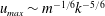 $u_{max}\sim m^{-1/6}k^{-5/6}$
for
$u_{max}\sim m^{-1/6}k^{-5/6}$
for
 $m\gg 1$
, i.e. the extremum decays with
$m\gg 1$
, i.e. the extremum decays with
 $m$
. For
$m$
. For
 $\unicode[STIX]{x1D6FF}\neq 0$
, the solution of (3.23) is corrected to
$\unicode[STIX]{x1D6FF}\neq 0$
, the solution of (3.23) is corrected to
 $\unicode[STIX]{x1D709}=(1-3\unicode[STIX]{x1D6FF}/2)\unicode[STIX]{x1D709}_{0}$
; that is, the time when the maximum of the solution is reached becomes shorter with increase of the ratio
$\unicode[STIX]{x1D709}=(1-3\unicode[STIX]{x1D6FF}/2)\unicode[STIX]{x1D709}_{0}$
; that is, the time when the maximum of the solution is reached becomes shorter with increase of the ratio
 $t_{2}/t_{1}$
.
$t_{2}/t_{1}$
.

Figure 3. Solution of (3.17) near the turning point
 $t_{\ast }$
; the maximum is achieved after passing through
$t_{\ast }$
; the maximum is achieved after passing through
 $t_{\ast }$
.
$t_{\ast }$
.
Finally, in order to determine the wavenumber for which the maximum of the solution is absolute, it should be noticed that this maximum corresponds to
 $m=1$
and is achieved after passing through the turning point
$m=1$
and is achieved after passing through the turning point
 $t_{\ast }$
, cf. figure 3, which is analogous to the bifurcation delay phenomena in dynamical systems if
$t_{\ast }$
, cf. figure 3, which is analogous to the bifurcation delay phenomena in dynamical systems if
 $s^{2}(t)$
is deemed to be a time-dependent bifurcation parameter. Given the general turning point solution with
$s^{2}(t)$
is deemed to be a time-dependent bifurcation parameter. Given the general turning point solution with
 $b=0$
, we can first determine where the maximum is achieved,
$b=0$
, we can first determine where the maximum is achieved,
 $$\begin{eqnarray}\frac{\text{d}}{\text{d}t}[\text{e}^{-t/8t_{\ast }}\text{Ai}(\unicode[STIX]{x1D70F})]=0\Rightarrow \frac{\text{Ai}(-\unicode[STIX]{x1D703}\widetilde{\unicode[STIX]{x1D70F}})}{\text{Ai}^{\prime }(-\unicode[STIX]{x1D703}\widetilde{\unicode[STIX]{x1D70F}})}=-8\unicode[STIX]{x1D703},\quad \unicode[STIX]{x1D703}=\frac{1}{2^{1/3}}\left(\frac{t_{1}}{t_{2}}\right)^{1/6},\,\unicode[STIX]{x1D70F}=\frac{t}{t_{1}},\end{eqnarray}$$
with
 $\unicode[STIX]{x1D703}\gg 1$
in case 4. Graphical analysis indicates that the solution of the above equation is near the first zero of
$\unicode[STIX]{x1D703}\gg 1$
in case 4. Graphical analysis indicates that the solution of the above equation is near the first zero of
 $\text{Ai}^{\prime }(-\unicode[STIX]{x1D703}\,\widetilde{\unicode[STIX]{x1D70F}})$
, denoted by
$\text{Ai}^{\prime }(-\unicode[STIX]{x1D703}\,\widetilde{\unicode[STIX]{x1D70F}})$
, denoted by
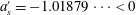 $a_{s}^{\prime }=-1.01879\cdots <0$
(Abramowitz & Stegun Reference Abramowitz and Stegun1965), which allows one to apply asymptotic methods to find the solution of (3.25),
$a_{s}^{\prime }=-1.01879\cdots <0$
(Abramowitz & Stegun Reference Abramowitz and Stegun1965), which allows one to apply asymptotic methods to find the solution of (3.25),
 $$\begin{eqnarray}\widetilde{\unicode[STIX]{x1D70F}}=-\frac{a_{s}^{\prime }}{\unicode[STIX]{x1D703}}+\widetilde{\unicode[STIX]{x1D70F}}^{\prime },\quad \text{where}~\widetilde{\unicode[STIX]{x1D70F}}^{\prime }=-\frac{1}{8\unicode[STIX]{x1D703}^{2}}\frac{\text{Ai}(a_{s}^{\prime })}{\text{Ai}^{\prime \prime }(a_{s}^{\prime })}+\cdots .\end{eqnarray}$$
By evaluating the solution at
 $\widetilde{\unicode[STIX]{x1D70F}}$
, i.e.
$\widetilde{\unicode[STIX]{x1D70F}}$
, i.e.
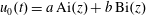
 $\widehat{f}^{\prime }(\widetilde{\unicode[STIX]{x1D70F}})=\text{const.}\,t_{2}^{1/2}\unicode[STIX]{x1D703}^{5/6}\text{e}^{-\widetilde{\unicode[STIX]{x1D70F}}/8}\text{Ai}(-\unicode[STIX]{x1D703}\,\widetilde{\unicode[STIX]{x1D70F}})$
, it is straightforward to show that there is no ‘optimum’ wavenumber
$\widehat{f}^{\prime }(\widetilde{\unicode[STIX]{x1D70F}})=\text{const.}\,t_{2}^{1/2}\unicode[STIX]{x1D703}^{5/6}\text{e}^{-\widetilde{\unicode[STIX]{x1D70F}}/8}\text{Ai}(-\unicode[STIX]{x1D703}\,\widetilde{\unicode[STIX]{x1D70F}})$
, it is straightforward to show that there is no ‘optimum’ wavenumber
 $k$
. Indeed, as
$k$
. Indeed, as
 $k\rightarrow 0$
,
$k\rightarrow 0$
,
 $$\begin{eqnarray}\widehat{f}^{\prime }(\widetilde{\unicode[STIX]{x1D70F}})\sim \unicode[STIX]{x1D703}^{5/6}\sim k^{-5/18},\end{eqnarray}$$
because
 $\text{Ai}(-\unicode[STIX]{x1D703}\widetilde{\unicode[STIX]{x1D70F}})\sim \text{const.}$
and
$\text{Ai}(-\unicode[STIX]{x1D703}\widetilde{\unicode[STIX]{x1D70F}})\sim \text{const.}$
and
 $\text{e}^{-\widetilde{\unicode[STIX]{x1D70F}}/8}\sim 1$
(since
$\text{e}^{-\widetilde{\unicode[STIX]{x1D70F}}/8}\sim 1$
(since
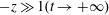
 $t_{1}\rightarrow +\infty$
for
$t_{1}\rightarrow +\infty$
for
 $k\rightarrow 0$
). As expected from the discussion in § 3.1, there is no critical self-similar wavenumber scaled with
$k\rightarrow 0$
). As expected from the discussion in § 3.1, there is no critical self-similar wavenumber scaled with
 $F^{-1}(t)$
and growing exponentially since, based on (3.26) and (3.27), the most amplified wavenumber at a given time
$F^{-1}(t)$
and growing exponentially since, based on (3.26) and (3.27), the most amplified wavenumber at a given time
 $t$
scales as
$t$
scales as
 $k\sim t^{-3/5}$
. Thus, the fundamental difference from the classical case
$k\sim t^{-3/5}$
. Thus, the fundamental difference from the classical case
 $Q=0$
is that no matter how small (but non-zero)
$Q=0$
is that no matter how small (but non-zero)
 $k$
is, there is a large enough time when this
$k$
is, there is a large enough time when this
 $k$
is amplified and then damped (for later times). It should be noted that for
$k$
is amplified and then damped (for later times). It should be noted that for
 $k\equiv 0$
, from (3.4a
) we find that
$k\equiv 0$
, from (3.4a
) we find that
 $a(t)=0$
,
$a(t)=0$
,
 $b(t)=-1/(4t^{2})$
and
$b(t)=-1/(4t^{2})$
and
 $s^{2}(t)=1/(4t^{2})$
, so that the leading-order solution reads as
$s^{2}(t)=1/(4t^{2})$
, so that the leading-order solution reads as
 $$\begin{eqnarray}u(t)=C_{1}t^{(1/2)+(1/\sqrt{2})}+C_{2}t^{(1/2)-(1/\sqrt{2})},\quad \text{and therefore}\quad \widehat{f}^{\prime }\sim t^{(1/2)+(1/\sqrt{2})},\end{eqnarray}$$
i.e. it grows faster than the undisturbed interface
 $F\sim t^{1/2}$
, in analogy with the Rayleigh–Taylor instability of an expanding sphere (Plesset Reference Plesset1954). The result (3.28) for
$F\sim t^{1/2}$
, in analogy with the Rayleigh–Taylor instability of an expanding sphere (Plesset Reference Plesset1954). The result (3.28) for
 $k\equiv 0$
contrasts with
$k\equiv 0$
contrasts with
 $\widehat{f}^{\prime }\sim t^{1/6}$
for
$\widehat{f}^{\prime }\sim t^{1/6}$
for
 $k\rightarrow 0$
, i.e. the limits
$k\rightarrow 0$
, i.e. the limits
 $k\rightarrow 0$
and
$k\rightarrow 0$
and
 $t\rightarrow \infty$
are not interchangeable and thus distinguished. Since the limit of
$t\rightarrow \infty$
are not interchangeable and thus distinguished. Since the limit of
 $k=0$
corresponds to a 2D problem, this transition from 3D to 2D makes some of the mechanisms (transfer of energy from the base state to the perturbation) disappear. Physically, a growing blob imminently breaks up in a finite time, and thus the range of finite non-zero wavenumbers amplified on this time scale ultimately affects the size of the resulting drops, which might be non-uniform due to the lack of a single preferred wavenumber.
$k=0$
corresponds to a 2D problem, this transition from 3D to 2D makes some of the mechanisms (transfer of energy from the base state to the perturbation) disappear. Physically, a growing blob imminently breaks up in a finite time, and thus the range of finite non-zero wavenumbers amplified on this time scale ultimately affects the size of the resulting drops, which might be non-uniform due to the lack of a single preferred wavenumber.
4 Effects of lateral acceleration
In addition to the radial acceleration due to
 $Q\neq 0$
, there could also be a lateral acceleration, e.g. due to the presence of gravity or, as in the case of a retracting soap film, due to the force pulling the cylinder in one direction. In the latter case, however, the Bond number
$Q\neq 0$
, there could also be a lateral acceleration, e.g. due to the presence of gravity or, as in the case of a retracting soap film, due to the force pulling the cylinder in one direction. In the latter case, however, the Bond number
 $Bo=\unicode[STIX]{x1D70C}F_{0}^{2}g/\unicode[STIX]{x1D70E}$
at the start of retraction (when the acceleration is the largest) of a film of thickness
$Bo=\unicode[STIX]{x1D70C}F_{0}^{2}g/\unicode[STIX]{x1D70E}$
at the start of retraction (when the acceleration is the largest) of a film of thickness
 $h$
is not small as
$h$
is not small as
 $Bo=F_{0}/h\geqslant 1$
; this is easy to see from the estimate of acceleration based on the Taylor–Culick theory,
$Bo=F_{0}/h\geqslant 1$
; this is easy to see from the estimate of acceleration based on the Taylor–Culick theory,
 $g\sim \unicode[STIX]{x1D70E}/(\unicode[STIX]{x1D70C}hF_{0})$
. The case of low Bond numbers in the soap film retraction corresponds only to the later stage of retraction when the blob has already grown and the acceleration diminishes as the blob approaches a constant Taylor–Culick speed
$g\sim \unicode[STIX]{x1D70E}/(\unicode[STIX]{x1D70C}hF_{0})$
. The case of low Bond numbers in the soap film retraction corresponds only to the later stage of retraction when the blob has already grown and the acceleration diminishes as the blob approaches a constant Taylor–Culick speed
 $\sqrt{2\unicode[STIX]{x1D70E}/\unicode[STIX]{x1D70C}h}$
, but by that time, the blob instability may have already developed. Here, we focus on the case of a weak acceleration due to external body forces such as gravity, so that
$\sqrt{2\unicode[STIX]{x1D70E}/\unicode[STIX]{x1D70C}h}$
, but by that time, the blob instability may have already developed. Here, we focus on the case of a weak acceleration due to external body forces such as gravity, so that
 $Bo\ll 1$
, which nevertheless leads to a modification of the base state and a contribution to the instability growth, analysed below with the help of (2.8).
$Bo\ll 1$
, which nevertheless leads to a modification of the base state and a contribution to the instability growth, analysed below with the help of (2.8).
4.1 Base state correction
From (2.8), it is obvious that non-zero acceleration
 $g$
affects mode
$g$
affects mode
 $n=1$
only and thus induces a non-axisymmetric flow field in the blob such as in figure 1(c),
$n=1$
only and thus induces a non-axisymmetric flow field in the blob such as in figure 1(c),
 $$\begin{eqnarray}L\widehat{f}_{1}^{\prime }=gF/2,\end{eqnarray}$$
which after the transformation
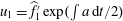 $u_{1}=\widehat{f}_{1}^{\prime }\,\text{exp}(\int a\,\text{d}t/2)$
reduces to
$u_{1}=\widehat{f}_{1}^{\prime }\,\text{exp}(\int a\,\text{d}t/2)$
reduces to
 $$\begin{eqnarray}u_{1}^{\prime \prime }-s^{2}(t)u_{1}=Ct^{1/2}gF(t)\equiv h(t),\quad \text{where}~s^{2}(t)=t^{-2}[4^{-1}-(t/t_{2})^{1/2}k^{2}F^{2}].\end{eqnarray}$$
Looking for a long-time correction, we can simplify
 $s^{2}(t)$
to
$s^{2}(t)$
to
 $s^{2}(t)=-t^{-1/2}t_{2}^{-1/2}t_{-1}<0$
, provided that
$s^{2}(t)=-t^{-1/2}t_{2}^{-1/2}t_{-1}<0$
, provided that
 $t\gg 4^{2/3}t^{2/3}t_{2}^{1/3}$
. The solution for the homogeneous part of (4.2) is
$t\gg 4^{2/3}t^{2/3}t_{2}^{1/3}$
. The solution for the homogeneous part of (4.2) is
 $$\begin{eqnarray}u_{1}(t)=\sqrt{t}Z_{2/3}\left({\textstyle \frac{4}{3}}t_{1}^{-1/2}t_{2}^{-1/4}t^{3/4}\right),\end{eqnarray}$$
where
 $Z_{\unicode[STIX]{x1D708}}(z)=C_{1}J_{\unicode[STIX]{x1D708}}(z)+C_{2}J_{-\unicode[STIX]{x1D708}}(z)$
,
$Z_{\unicode[STIX]{x1D708}}(z)=C_{1}J_{\unicode[STIX]{x1D708}}(z)+C_{2}J_{-\unicode[STIX]{x1D708}}(z)$
,
 $z=\unicode[STIX]{x1D6FE}t^{3/4}$
,
$z=\unicode[STIX]{x1D6FE}t^{3/4}$
,
 $\unicode[STIX]{x1D6FE}=(4/3)t_{1}^{-1/2}t_{2}^{-1/4}$
and
$\unicode[STIX]{x1D6FE}=(4/3)t_{1}^{-1/2}t_{2}^{-1/4}$
and
 $\unicode[STIX]{x1D708}=2/3$
. If
$\unicode[STIX]{x1D708}=2/3$
. If
 $u_{1}=C_{1}v_{1}+C_{2}v_{2}$
, with
$u_{1}=C_{1}v_{1}+C_{2}v_{2}$
, with
 $v_{1}=t^{1/2}J_{\unicode[STIX]{x1D708}}(z)$
and
$v_{1}=t^{1/2}J_{\unicode[STIX]{x1D708}}(z)$
and
 $v_{2}=t^{1/2}J_{-\unicode[STIX]{x1D708}}(z)$
, then the Wronskian is
$v_{2}=t^{1/2}J_{-\unicode[STIX]{x1D708}}(z)$
, then the Wronskian is
 $w=v_{1}v_{2}^{\prime }-v_{2}v_{1}^{\prime }$
and the solution to the inhomogeneous problem (4.2) reads
$w=v_{1}v_{2}^{\prime }-v_{2}v_{1}^{\prime }$
and the solution to the inhomogeneous problem (4.2) reads
 $$\begin{eqnarray}u_{1}(t)=v_{2}(t)\int ^{t}\frac{v_{1}(\unicode[STIX]{x1D70F})h(\unicode[STIX]{x1D70F})}{w(\unicode[STIX]{x1D70F})}\,\text{d}\unicode[STIX]{x1D70F}-v_{1}(t)\int ^{t}\frac{v_{2}(\unicode[STIX]{x1D70F})h(\unicode[STIX]{x1D70F})}{w(\unicode[STIX]{x1D70F})}\,\text{d}\unicode[STIX]{x1D70F}.\end{eqnarray}$$
Since we are considering the long-time limit, given the asymptotics (3.14), we can choose as independent solutions
 $v_{1}=t^{1/8}\text{e}^{\text{i}\unicode[STIX]{x1D6FE}t^{3/4}}$
and
$v_{1}=t^{1/8}\text{e}^{\text{i}\unicode[STIX]{x1D6FE}t^{3/4}}$
and
 $v_{2}=t^{1/8}\text{e}^{-\text{i}\unicode[STIX]{x1D6FE}t^{3/4}}$
, so that the Wronskian becomes constant,
$v_{2}=t^{1/8}\text{e}^{-\text{i}\unicode[STIX]{x1D6FE}t^{3/4}}$
, so that the Wronskian becomes constant,
 $w=-3\text{i}\unicode[STIX]{x1D6FE}/2$
, and the long-time limit of the solution (modulo a constant coefficient) is
$w=-3\text{i}\unicode[STIX]{x1D6FE}/2$
, and the long-time limit of the solution (modulo a constant coefficient) is
 $$\begin{eqnarray}u_{1}(t)\sim t^{1/8}\text{e}^{\text{i}\unicode[STIX]{x1D6FE}t^{3/4}}\int ^{t}\unicode[STIX]{x1D70F}^{9/8}\text{e}^{-\text{i}\unicode[STIX]{x1D6FE}\unicode[STIX]{x1D70F}^{3/4}}\,\text{d}\unicode[STIX]{x1D70F}-t^{1/8}\text{e}^{-\text{i}\unicode[STIX]{x1D6FE}t^{3/4}}\int ^{t}\unicode[STIX]{x1D70F}^{9/8}\text{e}^{\text{i}\unicode[STIX]{x1D6FE}\unicode[STIX]{x1D70F}^{3/4}}\,\text{d}\unicode[STIX]{x1D70F}\sim t^{3/2},\end{eqnarray}$$
where we took into account that the leading-order contribution of the integrals in the above expression can be evaluated through integration by parts,
 $$\begin{eqnarray}\int ^{t}\unicode[STIX]{x1D70F}^{9/8}\text{e}^{\text{i}\unicode[STIX]{x1D6FE}\unicode[STIX]{x1D70F}^{3/4}}\,\text{d}\unicode[STIX]{x1D70F}=-\text{i}\frac{4}{3\unicode[STIX]{x1D6FE}}t^{11/8}\text{e}^{\text{i}\unicode[STIX]{x1D6FE}t^{3/4}}+O(t^{5/8}).\end{eqnarray}$$
As a result, the correction to the base state scales with time
 $t$
, acceleration
$t$
, acceleration
 $g$
and mass flux
$g$
and mass flux
 $Q$
as
$Q$
as
 $u_{1}\sim g\sqrt{Q}t^{3/2}$
. For shorter times, i.e. when
$u_{1}\sim g\sqrt{Q}t^{3/2}$
. For shorter times, i.e. when
 $1/(4t^{2})$
dominates in
$1/(4t^{2})$
dominates in
 $s^{2}(t)$
, it is still the same mode
$s^{2}(t)$
, it is still the same mode
 $n=1$
that is excited, but with a different time exponent.
$n=1$
that is excited, but with a different time exponent.
4.2 Contribution to instability
Since lateral acceleration acts at all times, it makes sense to consider its contribution to instability at early times – if it boosts it, the effect will be observable. From (2.8), we see that the axisymmetric mode is affected by mode one through the presence of acceleration
 $g$
,
$g$
,
 $$\begin{eqnarray}L\widehat{f}_{0}^{\prime }=g(\widehat{f}_{-1}^{\prime }+\widehat{f}_{1}^{\prime })/2=g\widehat{f}_{1}^{\prime },\end{eqnarray}$$
where we took into account the symmetry
 $n\rightarrow -n$
and
$n\rightarrow -n$
and
 $\widehat{f}_{1}^{\prime }$
is determined from the homogeneous equation
$\widehat{f}_{1}^{\prime }$
is determined from the homogeneous equation
 $L\widehat{f}_{1}^{\prime }=0$
or, after the transformation
$L\widehat{f}_{1}^{\prime }=0$
or, after the transformation
 $\widehat{f}_{1}^{\prime }=\text{exp}(-\!\int a\,\text{d}t/2)u_{1}=t^{-1/2}u_{1}$
corresponding to
$\widehat{f}_{1}^{\prime }=\text{exp}(-\!\int a\,\text{d}t/2)u_{1}=t^{-1/2}u_{1}$
corresponding to
 $a(t)=1/t$
, from (3.3) with
$a(t)=1/t$
, from (3.3) with
 $n=1$
. For short times,
$n=1$
. For short times,
 $s^{2}(t)=1/(4t^{2})$
, and hence the leading-order solution of (3.3) is
$s^{2}(t)=1/(4t^{2})$
, and hence the leading-order solution of (3.3) is
 $u_{1}(t)\sim t^{(1/2)+(1/\sqrt{2})}$
, so that
$u_{1}(t)\sim t^{(1/2)+(1/\sqrt{2})}$
, so that
 $\widehat{f}_{1}^{\prime }\sim t^{1/\sqrt{2}}$
. To construct the solution to (4.7), we make the transformation
$\widehat{f}_{1}^{\prime }\sim t^{1/\sqrt{2}}$
. To construct the solution to (4.7), we make the transformation
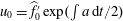 $u_{0}=\widehat{f}_{0}^{\prime }\,\text{exp}(\int a\,\text{d}t/2)$
, where
$u_{0}=\widehat{f}_{0}^{\prime }\,\text{exp}(\int a\,\text{d}t/2)$
, where
 $a=1/(4t_{1})$
, to produce
$a=1/(4t_{1})$
, to produce
 $$\begin{eqnarray}u_{0}^{\prime \prime }-s^{2}(t)u_{0}=\text{e}^{-t/8t_{1}}g\,\widehat{f}_{1}^{\prime }/2\equiv h(t)\sim g\text{e}^{-t/8t_{1}}t^{1/\sqrt{2}}.\end{eqnarray}$$
Since for short times
 $s^{2}(t)=1/(4t^{2})$
, two independent solutions of the homogeneous part are
$s^{2}(t)=1/(4t^{2})$
, two independent solutions of the homogeneous part are
 $$\begin{eqnarray}u_{0}(t)=C_{1}v_{1}+C_{2}v_{2},\quad \text{with}~v_{1}(t)=t^{(1/2)+(1/\sqrt{2})},\,v_{2}(t)=t^{(1/2)-(1/\sqrt{2})},\end{eqnarray}$$
i.e. given by case 2, and the Wronskian
 $w=-\sqrt{2}$
. Using formula (4.4), the corresponding perturbation driven by acceleration
$w=-\sqrt{2}$
. Using formula (4.4), the corresponding perturbation driven by acceleration
 $g$
is then to leading order given by
$g$
is then to leading order given by
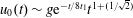 $u_{0}(t)\sim g\text{e}^{-t/8t_{1}}t^{1+(1/\sqrt{2})}$
, i.e.
$u_{0}(t)\sim g\text{e}^{-t/8t_{1}}t^{1+(1/\sqrt{2})}$
, i.e.
 $\widehat{f}_{0}^{\prime }=t^{1+(1/\sqrt{2})}$
, and thus the (algebraic) growth is faster than that in the absence of acceleration, which is
$\widehat{f}_{0}^{\prime }=t^{1+(1/\sqrt{2})}$
, and thus the (algebraic) growth is faster than that in the absence of acceleration, which is
 $t^{(1+\sqrt{2})/2}\text{e}^{t/8t_{1}}$
. Here, the exponential should be discarded as
$t^{(1+\sqrt{2})/2}\text{e}^{t/8t_{1}}$
. Here, the exponential should be discarded as
 $t\ll t_{1}$
according to the case 2 assumptions. Hence, the presence of lateral acceleration entails amplification of the instability at early times without changing the wavenumber structure of the perturbation.
$t\ll t_{1}$
according to the case 2 assumptions. Hence, the presence of lateral acceleration entails amplification of the instability at early times without changing the wavenumber structure of the perturbation.
5 Discussion and further questions
In this paper, we considered the case in which the time scale for the growth of the liquid blob is commensurate with the intrinsic time scale for the instability in the static situation, so that quasistatic analyses and the idea of a time-varying critical wavenumber fail. Linearization of the basic equations about the axisymmetric base state produces a non-autonomous non-homogeneous oscillator equation (2.8). The results show that no matter how small the wavenumber
 $k$
is, the apparent growth of the corresponding mode is illusory, as all of the modes ultimately evolve to decaying oscillations after passing through a turning point in time
$k$
is, the apparent growth of the corresponding mode is illusory, as all of the modes ultimately evolve to decaying oscillations after passing through a turning point in time
 $t_{\ast }$
at which the time-dependent ‘spring constant’
$t_{\ast }$
at which the time-dependent ‘spring constant’
 $s^{2}(t)$
changes sign. Furthermore, this time increases unboundedly for
$s^{2}(t)$
changes sign. Furthermore, this time increases unboundedly for
 $k\rightarrow 0$
. Qualitatively, the ultimate decay of the perturbation can be predicted from the classical theory, in which the unstable wavelengths
$k\rightarrow 0$
. Qualitatively, the ultimate decay of the perturbation can be predicted from the classical theory, in which the unstable wavelengths
 $\unicode[STIX]{x1D706}=2\unicode[STIX]{x03C0}/k$
correspond to
$\unicode[STIX]{x1D706}=2\unicode[STIX]{x03C0}/k$
correspond to
 $\unicode[STIX]{x1D706}>2\unicode[STIX]{x03C0}F$
, i.e. should be greater than the circumference of the blob. If at a given instant of time a perturbation of a particular wavelength
$\unicode[STIX]{x1D706}>2\unicode[STIX]{x03C0}F$
, i.e. should be greater than the circumference of the blob. If at a given instant of time a perturbation of a particular wavelength
 $\unicode[STIX]{x1D706}^{\ast }$
in that range is expected to grow, at later time it is pushed back to the stable range
$\unicode[STIX]{x1D706}^{\ast }$
in that range is expected to grow, at later time it is pushed back to the stable range
 $\unicode[STIX]{x1D706}^{\ast }<2\unicode[STIX]{x03C0}F(t)$
due to the growth of
$\unicode[STIX]{x1D706}^{\ast }<2\unicode[STIX]{x03C0}F(t)$
due to the growth of
 $F(t)$
. Hence, several ‘standard’ assumptions based on the direct translation of the classical theory onto the time-varying case – exponential growth of perturbations and time-varying wavenumber – are generally invalid. These seemingly counterintuitive results can be foreseen from the simple fact that in 3D, in general, there is no conformal (i.e. angle preserving) mapping that leaves the Laplace equation (2.1a
) invariant. The exceptions – translations and homogeneous scalings, rotations and reflections, and inversions – known from Liouville’s theorem (Blair Reference Blair2000) obviously do not apply to the growing cylindrical blob considered here, thus making the presented theory non-conformal (Blumenhagen & Plauschinn Reference Blumenhagen and Plauschinn2009). If such a mapping – between a growing and a static blob problem – parameterized by time
$F(t)$
. Hence, several ‘standard’ assumptions based on the direct translation of the classical theory onto the time-varying case – exponential growth of perturbations and time-varying wavenumber – are generally invalid. These seemingly counterintuitive results can be foreseen from the simple fact that in 3D, in general, there is no conformal (i.e. angle preserving) mapping that leaves the Laplace equation (2.1a
) invariant. The exceptions – translations and homogeneous scalings, rotations and reflections, and inversions – known from Liouville’s theorem (Blair Reference Blair2000) obviously do not apply to the growing cylindrical blob considered here, thus making the presented theory non-conformal (Blumenhagen & Plauschinn Reference Blumenhagen and Plauschinn2009). If such a mapping – between a growing and a static blob problem – parameterized by time
 $t$
were to exist, then there would also exist a most unstable wavenumber that scales with time.
$t$
were to exist, then there would also exist a most unstable wavenumber that scales with time.
Therefore, a growing blob is expected to rupture in a manner different from a static blob with one preferred wavelength. In the natural scenario, when one starts with random initial conditions with no preferred wavelength, then a range of wavelengths, determined by the time scale of the cylinder rupture (or, at least, by the time it takes for the amplitude of perturbations to become finite and comparable to the cylinder radius, thus triggering nonlinear mechanisms), will be amplified. Since perturbations with different wavelengths in this range would also have random phase shifts between them, then the resulting drop sizes should not be uniform. In the other scenario, when one provides an initial modulation with a particular wavelength, such as in the experiments of Donnelly & Glaberson (Reference Donnelly and Glaberson1966), who verified the classical dispersion relation (3.5), the breakup may result in a uniform size of the drops. At this point, there are no experiments (yet) which would be directly comparable to the offered theory. The closest phenomena would be along-the-edge instability of retracting soap films, but, as was mentioned above, the Bond numbers in that case are greater than or equal to one at the start of retraction. The case of low Bond numbers in the soap film retraction corresponds only to the later stage of retraction when the blob is already massive and the acceleration decreases as the blob approaches a constant Taylor–Culick speed, but by that time an instability would have already developed. Should the presented theory be applicable in that case, it would predict that the lateral acceleration would amplify the instability at early times without changing the wavenumber structure of the perturbation. Any future experiment would have to deliver sufficiently high-fidelity data to be able to distinguish non-exponential growths predicted by the theory and, instead of focusing on an average wavelength of perturbation as commonly done, pay attention to the large scatter around the average, which is indicative of a range of wavelengths amplified, thus leading to breakup at different drop sizes. It would also be interesting to observe, e.g. through an initial modulation, the wavenumbers that initially grow and then decay in an oscillating fashion as in figure 2.
In conclusion, it is worth noting that the transient growth of the perturbation observed in figure 2 is a consequence of both the non-normal and non-autonomous nature of the linear operator of the homogeneous part of (2.7). Once the perturbation amplitude becomes finite, nonlinear advection terms
 $(\boldsymbol{v}\boldsymbol{\cdot }\unicode[STIX]{x1D735})\boldsymbol{v}$
in the Euler equations must be taken into account, which affect not only the amplitude of the disturbance, but also its direction, due to the gradient operator
$(\boldsymbol{v}\boldsymbol{\cdot }\unicode[STIX]{x1D735})\boldsymbol{v}$
in the Euler equations must be taken into account, which affect not only the amplitude of the disturbance, but also its direction, due to the gradient operator
 $\unicode[STIX]{x1D735}$
, thus influencing the eventual breakup process. All of these aspects are beyond the scope of the present analysis. While the case of
$\unicode[STIX]{x1D735}$
, thus influencing the eventual breakup process. All of these aspects are beyond the scope of the present analysis. While the case of
 $Q=\text{const.}$
considered in detail here provides a roadmap to the instability development for a growing cylindrical blob, it would also be interesting to extend the present study to a time-varying mass flux
$Q=\text{const.}$
considered in detail here provides a roadmap to the instability development for a growing cylindrical blob, it would also be interesting to extend the present study to a time-varying mass flux
 $Q=Q(t)$
, in particular to understand the stability of time-periodic
$Q=Q(t)$
, in particular to understand the stability of time-periodic
 $Q(t)$
amenable to Floquet analysis and to find a way to suppress instability by controlling the form of
$Q(t)$
amenable to Floquet analysis and to find a way to suppress instability by controlling the form of
 $Q(t)$
. Moreover, the influence of viscosity has been omitted in the present analysis, although its inclusion should not be a serious undertaking in the linear approximation (Levich Reference Levich1962). Finally, evaluation of the effect of displacement of the line source off the symmetry axis, while expected to enhance instability because the amplitude of
$Q(t)$
. Moreover, the influence of viscosity has been omitted in the present analysis, although its inclusion should not be a serious undertaking in the linear approximation (Levich Reference Levich1962). Finally, evaluation of the effect of displacement of the line source off the symmetry axis, while expected to enhance instability because the amplitude of
 $I_{n}$
increases towards the surface where the Rayleigh–Plateau instability is generated, would be important for quantitative understanding of various problems such as retracting liquid (soap) sheets, where the coupling between the liquid sheet and the rim in previous works (e.g. Agbaglah et al.
Reference Agbaglah, Josserand and Zaleski2013) is usually considered through the variation of the rim radius only, i.e. without actual interaction between the rim and the sheet.
$I_{n}$
increases towards the surface where the Rayleigh–Plateau instability is generated, would be important for quantitative understanding of various problems such as retracting liquid (soap) sheets, where the coupling between the liquid sheet and the rim in previous works (e.g. Agbaglah et al.
Reference Agbaglah, Josserand and Zaleski2013) is usually considered through the variation of the rim radius only, i.e. without actual interaction between the rim and the sheet.
Acknowledgements
This work was partially supported by a National Science Foundation (NSF) CAREER award under grant no. 1054267 and the Natural Sciences and Engineering Research Council of Canada (NSERC) under grant no. 6186. The author would also like to thank A. Zelnikov for stimulating discussions.


