2. Model

We consider a uniformly heated layer of fluid bounded between two horizontal plates at a vertical distance $d$. The fluid has kinematic viscosity $\nu$, thermal diffusivity $\kappa$, density $\rho$, specific heat capacity $c_p$, and thermal expansion coefficient $\alpha$. The dimensional heating rate per unit volume $Q$ is constant in time and space. For simplicity, we assume that the layer is periodic in the horizontal ($x$ and $y$) directions, with periods $L_x$ and $L_y$. While these values affect the mean vertical heat flux, the analytical bounds derived below do not depend on $L_x$ or $L_y$ and therefore apply to domains of all sizes (including the limiting case of a horizontally infinite fluid layer).

To make the problem non-dimensional, we use $d$ as the characteristic length scale, $d^{2}/\kappa$ as the time scale and $d^{2}Q/\kappa \rho c_p$ as the temperature scale. The motion of the fluid in the non-dimensional domain $\varOmega = [0,L_x] \times [0,L_y] \times [0,1]$ is then governed by the Boussinessq equations

(2.1a)$$\begin{gather} \boldsymbol{\nabla} \boldsymbol{\cdot} \boldsymbol{u} = 0, \end{gather}$$

(2.1b)$$\begin{gather}\partial_t \boldsymbol{u}+ \boldsymbol{u}\boldsymbol{\cdot} \boldsymbol{\nabla} \boldsymbol{u} + \boldsymbol{\nabla} p = {\textit{Pr}} ({\nabla}^{2}\boldsymbol{u} + {\textit{R}} T \boldsymbol{\hat{\boldsymbol{z}}}), \end{gather}$$

(2.1c)$$\begin{gather}\partial_t T + \boldsymbol{u}\boldsymbol{\cdot} \boldsymbol{\nabla} T = {\nabla}^{2}T + 1, \end{gather}$$

where $\boldsymbol {u}$ is the fluid velocity, $p$ is the pressure, and the unit forcing in (2.1c) represents the non-dimensional internal heating rate. The no-slip, fixed-flux boundary conditions are expressed by

(2.2a)$$\begin{gather} \left.{\boldsymbol{u}}\right\rvert_{z=0}^{} = \left.{\boldsymbol{u}}\right\rvert_{z=1}^{} =0, \end{gather}$$

(2.2b)$$\begin{gather}\left.{\partial_z T}\right\rvert_{z=0}^{} = 0, \quad\left.{\partial_z T}\right\rvert_{z=1}^{} ={-}1. \end{gather}$$

The dimensionless quantities

(2.3a,b)\begin{equation} {\textit{Pr}} = \frac{\nu}{\kappa} \quad\text{and}\quad {\textit{R}} = \frac{g \alpha Q d^{5}}{\rho c_p \nu \kappa^{2}}, \end{equation}

where $g$ is the acceleration of gravity, are the only two non-dimensional control parameters. The former is the usual Prandtl number, which measures the ratio of momentum and heat diffusivity. The latter, instead, measures the destabilising effect of internal heating compared with the stabilising effects of diffusion, and may therefore be interpreted as a Rayleigh number.

Since the volume-averaged temperature $\int\kern-8pt - T(\boldsymbol {x},t) \textrm {d}\kern0.06em \boldsymbol {x}$ is conserved in time, we assume it to be zero without loss of generality. With this extra condition, the governing equations admit the solution $\boldsymbol {u}=\boldsymbol {0}$, $p = \text {constant}$ and $T = -({z^{2}}/{2}) + \frac 16$ at all $ {\textit {R}}$, which represents a purely conductive state. This state is globally asymptotically stable irrespective of the horizontal periods $L_x$ and $L_y$ if $ {\textit {R}} < 1429.86$, and it is linearly unstable when $ {\textit {R}} > 1440$ for sufficiently large horizontal periods (Goluskin Reference Goluskin2015). Convection ensues above this Rayleigh number for at least one choice of the horizontal periods, and cannot currently be ruled out above the known global stability threshold. We are therefore interested in bounds on $\langle wT \rangle$ that hold for arbitrary $ {\textit {R}} \geq 1429.86$.

3. Bounding framework

To derive an upper bound on $\langle wT \rangle$, it is convenient to lift the inhomogeneous boundary condition on the temperature by introducing the temperature perturbation

(3.1)\begin{equation} \theta(\boldsymbol{x},t) = T(\boldsymbol{x},t) + \frac{z^{2}}{2} -\frac 16. \end{equation}

The heat equation (2.1c) and boundary conditions (2.2b) show that $\theta$ satisfies

(3.2a)$$\begin{gather} \partial_t \theta + \boldsymbol{u}\boldsymbol{\cdot} \boldsymbol{\nabla} \theta = {\nabla}^{2}\theta + z w, \end{gather}$$

(3.2b)$$\begin{gather}\left.{\partial_z\theta}\right\rvert_{z=0}^{} = 0, \quad\left.{\partial_z\theta}\right\rvert_{z=1}^{} = 0. \end{gather}$$

To rewrite the heat flux in terms of $\theta$, observe that, by virtue of incompressibility and of the boundary conditions in (2.2a), the horizontal-and-time average $\bar {w}(z)$ of the vertical velocity $w$ vanishes for all $z$. Then

(3.3)\begin{equation} \langle w f(z) \rangle= \int_0^{1} \bar{w}(z) f(z) \, \textrm{d}z = 0 \end{equation}

for any $z$-dependent function $f(z)$, and in particular we conclude that

(3.4)\begin{equation} \langle wT \rangle = \langle w\theta \rangle. \end{equation}

A rigorous upper bound on $\langle w\theta \rangle$ can be derived using the auxiliary functional method (Chernyshenko et al. Reference Chernyshenko, Goulart, Huang and Papachristodoulou2014) with the quadratic auxiliary functional

(3.5)\begin{equation} \mathcal{V}\{\boldsymbol{u}, \theta \} = \int\kern-8pt -_{\varOmega} \frac{a}{2 {\textit{Pr}} {\textit{R}}} |\boldsymbol{u}|^{2} + \frac{b}{2} |\theta|^{2} - \phi(\boldsymbol{x}) \theta - \boldsymbol{\psi}(\boldsymbol{x}) \boldsymbol{\cdot} \boldsymbol{u}\,\textrm{d}\kern0.06em \boldsymbol{x}, \end{equation}

where the non-negative scalars $a$ and $b$, the function $\phi$ and the vector field $\boldsymbol {\psi }$ are to be optimised in order to obtain the best possible bound. Chernyshenko (Reference Chernyshenko2017) showed that this is equivalent to employing the background method: the profile ${\phi }/{b}$ is the background temperature (defined with respect to $\theta$), the vector field $({Pr R}/{a}) \boldsymbol {\psi }$ is the background velocity, and $a$ and $b$ are the so-called balance parameters. Contrary to the classical background method, there is no need to impose boundary or incompressibility conditions on $\boldsymbol {\psi }$ or $\phi$ when defining $\mathcal {V}$. To simplify the analysis below, however, we take $\boldsymbol {\psi }$ to be incompressible, horizontally periodic and vanishing at the top and bottom plates. The optimality of these choices can be proved rigorously, but the details are beyond the scope of this work.

Arguments identical to those given by Goluskin & Fantuzzi (Reference Goluskin and Fantuzzi2019, appendix A) show that the auxiliary function (3.5) may be taken to be invariant under arbitrary horizontal translations and under the ‘horizontal flow reversal’ variable transformation

(3.6a,b)\begin{equation} \begin{pmatrix}\boldsymbol{u}(\boldsymbol{x},t)\\ \theta(\boldsymbol{x},t) \\ p(\boldsymbol{x},t)\end{pmatrix} \mapsto \begin{pmatrix} \mathsf{G} \boldsymbol{u}(\mathsf{G}\boldsymbol{x},t)\\ \theta(\mathsf{G}\boldsymbol{x},t) \\ p(\mathsf{G}\boldsymbol{x},t)\end{pmatrix},\qquad \mathsf{G}= \begin{pmatrix}-1 & 0 & 0\\ 0 & -1 & 0\\ 0 & 0 & 1\end{pmatrix}. \end{equation}

This is because the governing equations (2.1a), (2.1b) and (3.2a) are invariant under the same set of transformations. Invariance under horizontal translation requires $\phi (\boldsymbol {x})=\phi (z)$ and $\boldsymbol {\psi }(\boldsymbol {x})=\boldsymbol {\psi }(z)$. In particular, the incompressibility and no-slip conditions on $\boldsymbol {\psi }$ imply that we must have $\boldsymbol {\psi }(z) = (\psi _1(z), \psi _2(z), 0)$. Invariance under (3.6a,b) then requires $\psi _1(z)=\psi _2(z)=0$, so $\boldsymbol {\psi }=\boldsymbol {0}$.

Making these restrictions from now on, it can be shown that $\mathcal {V}\{\boldsymbol {u}(t), \theta (t) \}$ remains uniformly bounded in time along solutions of (2.1b) and (3.2a) for any given initial velocity and temperature. We can therefore use the fundamental theorem of calculus and the governing equations to write

(3.7) \begin{align} \langle w \theta \rangle &= \limsup_{\tau \rightarrow \infty}\frac{1}{\tau} \int_{0}^{\tau} \int\kern-8pt -_{\varOmega} w\theta + \frac{\textrm{d}}{ \textrm{d}t}\mathcal{V}\{\boldsymbol{u}(t),\theta(t)\}\,\textrm{d}\kern0.7pt\boldsymbol{x}\,\textrm{d}t \nonumber\\ &= \limsup_{\tau \rightarrow \infty}\frac{1}{\tau} \int_{0}^{\tau} \int\kern-8pt -_{\varOmega} w\theta + \frac{a}{ {\textit{Pr}} {\textit{R}}}\boldsymbol{u} \boldsymbol{\cdot} \partial_t \boldsymbol{u} + b \theta \partial_t \theta - \phi(z)\partial_t \theta \,\textrm{d}\kern0.06em\boldsymbol{x}\,\textrm{d}t \nonumber\\ &= U -\liminf_{\tau \rightarrow \infty}\frac{1}{\tau} \int_{0}^{\tau} \mathcal{S}\{\boldsymbol{u}(t),\theta(t) \} \,\textrm{d}t \end{align}

for any constant $U$, where

(3.8)\begin{equation} \mathcal{S}\{\boldsymbol{u},\theta\} = \int\kern-8pt -_{\varOmega} \frac{a}{R}|\boldsymbol{\nabla}\boldsymbol{u}|^{2} + b |\boldsymbol{\nabla} \theta|^{2} - (a+1 +bz - \phi' )w\theta -\phi' \partial_z\theta + U\, \textrm{d}\kern0.06em\boldsymbol{x} \end{equation}

and primes denote derivatives with respect to $z$. The last equality in (3.7) is obtained after a few integrations by parts that exploit the boundary conditions, incompressibility and the identity (3.3). The bound $\langle w T \rangle = \langle w\theta \rangle \leq U$ follows from (3.4) and (3.7) if $\mathcal {S}\{\boldsymbol {u},\theta \}$ is non-negative for all time-independent velocities $\boldsymbol {u}$ and temperature perturbations $\theta$ that satisfy incompressibility and the boundary conditions in (2.2a) and (3.2b). Our goal, therefore, is to choose $a$, $b$ and $\phi (z)$ such that this condition holds for the smallest possible $U$.

To simplify this task, we invoke the horizontal periodicity and expand the velocity and temperature fields using Fourier series:

(3.9)\begin{equation} \begin{bmatrix} \theta(x,y,z)\\ \boldsymbol{u}(x,y,z) \end{bmatrix} = \sum_{\boldsymbol{k}} \begin{bmatrix} \hat{\theta}_{\boldsymbol{k}}(z)\\ \hat{\boldsymbol{u}}_{\boldsymbol{k}}(z) \end{bmatrix} \exp({\textrm{i}(k_x x + k_y y)}). \end{equation}

The sum is over wavevectors $\boldsymbol {k}=(k_x,k_y)$ of magnitude $k = \sqrt {k_{\smash {x}}^{2} + k_{\smash {y}}^{2}}$ that are compatible with the horizontal periods $L_x$ and $L_y$. The (complex-valued) Fourier amplitudes $\hat {\theta }_{\boldsymbol {k}}$ and $\hat {\boldsymbol {u}}_{\boldsymbol {k}}=(\hat {u}_{\boldsymbol {k}}, \hat {v}_{\boldsymbol {k}},\hat {w}_{\boldsymbol {k}})$ satisfy

(3.10a)$$\begin{gather} \hat{u}_{\boldsymbol{k}}(0) = \hat{u}_{\boldsymbol{k}}(1)= \hat{v}_{\boldsymbol{k}}(0) = \hat{v}_{\boldsymbol{k}}(1)=0, \end{gather}$$

(b)$$\begin{gather}\hat{w}_{\boldsymbol{k}}(0) = \hat{w}_{\boldsymbol{k}}'(0) = \hat{w}_{\boldsymbol{k}}(1) = \hat{w}_{\boldsymbol{k}}'(1)= 0, \end{gather}$$

(3.10c)$$\begin{gather}\hat{\theta}_{\boldsymbol{k}}'(0)=\hat{\theta}_{\boldsymbol{k}}'(1) = 0. \end{gather}$$

After substituting (3.9) into (3.8), the Fourier-transformed incompressibility condition $ik_x \hat {u}_{\boldsymbol {k}} + ik_y \hat {v}_{\boldsymbol {k}} + \hat {w}_{\boldsymbol {k}}' = 0$ can be combined with Young's inequality to estimate

(3.11)\begin{equation} \mathcal{S}\{\boldsymbol{u},\theta\} \geq \mathcal{S}_{0}\{\hat{\theta}_0\} + \sum_{\boldsymbol{k}} \mathcal{S}_{\boldsymbol{k}} \{\hat{w}_{\boldsymbol{k}}, \hat{\theta}_{\boldsymbol{k}}\}, \end{equation}

where

(3.12a)\begin{equation} \mathcal{S}_0\{\hat{\theta}_0\}:= U + \int^{1}_{0} b|\hat{\theta}'_0(z)|^{2} - \phi'\hat{\theta}'_0(z)\,\textrm{d}z \end{equation}

and

(3.12b)\begin{align} \mathcal{S}_{\boldsymbol{k}}\{\hat{w}_{\boldsymbol{k}},\hat{\theta}_{\boldsymbol{k}}\} := \int^{1}_{0} \frac{a}{R}\left(\frac{|\hat{w}''_{\boldsymbol{k}}(z)|^{2}}{k^{2}} + 2|\hat{w}'_{\boldsymbol{k}}(z)|^{2} + k^{2}|\hat{w}_{\boldsymbol{k}}(z)|^{2} \right) +b|\hat{\theta}'_{\boldsymbol{k}}(z)|^{2} \nonumber\\ + bk^{2}|\hat{\theta}_{\boldsymbol{k}}(z)|^{2} - [a+1+bz - \phi'(z)]\hat{w}_{\boldsymbol{k}}(z)^{*}\hat{\theta}_{\boldsymbol{k}}(z) \, \textrm{d}z. \end{align}

Standard arguments (see e.g. Arslan et al. Reference Arslan, Fantuzzi, Craske and Wynn2021) show that the right-hand side of (3.11) is non-negative if and only if each summand is non-negative, and that to check these conditions one can assume that $\hat {w}_{\boldsymbol {k}}$ and $\hat {\theta }_{\boldsymbol {k}}$ are real functions. Thus, the best bound on $\langle w T \rangle$ is found upon solving the optimisation problem

(3.13) \begin{equation} \begin{aligned} \inf_{U,\phi'(z),a,b} \{U:\quad & \mathcal{S}_0\{\hat{\theta}_0\} \geq 0 \quad\forall\ \hat{\theta}_0 \text{ s.t. } (3.10c),\\ & \mathcal{S}_{\boldsymbol{k}}\{\hat{w}_{\boldsymbol{k}},\hat{\theta}_{\boldsymbol{k}}\} \geq 0 \quad\forall\ \hat{w}_{\boldsymbol{k}},\hat{\theta}_{\boldsymbol{k}} \text{ s.t. }(3.10a), \forall \boldsymbol{k}\neq 0\}. \end{aligned} \end{equation}

We refer to the condition $\mathcal {S}_{\boldsymbol {k}}\{\hat {w}_{\boldsymbol {k}},\hat {\theta }_{\boldsymbol {k}}\} \geq 0$ as the spectral constraint and consider $\phi '$, rather than $\phi$, as the optimisation variable because only the former appears in the problem.

4. Analytical bound

To derive an analytical bound on $\langle wT \rangle$, we begin by observing that

(4.1)\begin{equation} \mathcal{S}_0\{\hat{\theta}_0\} = \int^{1}_{0} b\left(\hat{\theta}'_{0}(z) - \frac{\phi'(z)}{2b} \right)^{2} - \frac{\phi'(z)^{2}}{4b} + U\, \textrm{d}z \geq U - \int^{1}_{0}\frac{\phi'(z)^{2}}{4b}\textrm{d}z, \end{equation}

so the constraint on $\mathcal {S}_0$ in (3.13) is satisfied if we choose

(4.2)\begin{equation} U = \int^{1}_{0}\frac{\phi'(z)^{2}}{4b}\,\textrm{d}z. \end{equation}

This choice is also optimal because the lower bound in (4.1) is sharp. To see this, let $\hat {\theta }_0$ be such that $\hat {\theta }_0'(z) = ({1}/{2b})\phi '(z)$ except for boundary layers of width $\epsilon$ near $z=0$ and $z=1$, where $\hat {\theta }_0'(z)=0$ to satisfy (3.10c). Then, let $\epsilon \to 0$ and apply Lebesgue's dominated convergence theorem to conclude that $\mathcal {S}\{\hat{\theta}_{0}\}$ converges to the right-hand side of (4.1).

Next, we seek constants $a$ and $b$ and a function $\phi (z)$ that minimise the right-hand side of (4.2) whilst satisfying the spectral constraint in (3.13). The simplest way to ensure this is to set $\phi '(z)=a+1+bz$, because then the only sign-indefinite term in $\mathcal {S}_{\boldsymbol {k}}$ vanishes. This choice yields

(4.3)\begin{equation} \langle wT \rangle \leq U = \frac{1}{12} \left[ b + 3(a+1) + \frac{(a+1)^{2}}{b} \right], \end{equation}

which attains the minimum value of $\frac {1}{2}(\frac {1}{2} + \frac {1}{\sqrt {3}})$ when $b=\sqrt {3}(a+1)$ and $a=0$.

While this simple construction already halves the uniform bound proved by Goluskin (Reference Goluskin2016), an even better result that depends explicitly on the Rayleigh number can be obtained by letting $\phi '$ develop boundary layers of width $\delta$ near $z=0$ and $z=1$. Specifically, we still fix

(4.4)\begin{equation} b = \sqrt{3}(a+1), \end{equation}

but this time take

(4.5a,b)\begin{equation} \phi '(z) = (a + 1)\xi (z),\quad \xi (z) = \left\{ \begin{array}{l} \left( {\frac{1}{\delta } + \sqrt 3 } \right)z,\,\,\,\,\,\,\,\,\,\,\,\,\,\,\,\,\,\,\,\,\,\,\,\,0 \le z \le \delta ,\\1 + \sqrt 3 {\mkern 1mu} z,\,\,\,\,\,\,\,\,\,\,\,\,\,\,\,\,\,\,\,\,\,\,\,\,\,\,\,\,\,\,\,\,\delta \le z \le 1 - \delta ,\\ \left( {\frac{{1 + \sqrt 3 }}{\delta } - \sqrt 3 } \right)(1 - z),\,\,\,\,\,1 - \delta \le z \le 1. \end{array} \right. \end{equation}

This profile, illustrated in figure 2, yields the upper bound

(4.6a)\begin{align} \langle wT \rangle \leq U &= \frac 12 \left(\frac 12 + \frac{1}{\sqrt{3}} - \frac{6+5\sqrt{3}}{9}\delta + \frac{\sqrt{3}}{6}\delta^{2} \right) (a+1) \end{align}

(4.6b)\begin{align} &\leq \frac 12 \left( \frac 12 + \frac{1}{\sqrt{3}} - A\delta \right) (a+1), \end{align}

where the last inequality holds for any constant $A$ satisfying $A \leq \frac {1}{9}(6 + 5\sqrt {3}) - \frac {\sqrt {3}}{6}\delta$. Anticipating that the height of the boundary layers in $\phi '$ will have to be small, we arbitrarily assume that $\delta \leq \frac{1}{3}$ (this will be checked a posteriori) and therefore set $A = (4+3\sqrt {3})/6$ irrespective of $\delta$. These conservative choices considerably simplify the algebra in what follows.

Figure 2. Sketch of the piecewise linear $\phi '(z)$ in (4.5a,b).

Note that although (4.2) suggests setting $\xi (z)=0$ throughout the boundary layers, a linear variation makes the spectral constraint easier to satisfy and results in a smaller bound on $\langle wT \rangle$. The values of $a$ and $\delta$ must be chosen as functions of $ {\textit {R}}$ to minimise (4.6b) whilst ensuring that the indefinite term in $\mathcal {S}_{\boldsymbol {k}}$,

(4.7)\begin{equation} \mathcal{I} := (a+1)\int_{[0,\delta]\cup[1-\delta,1]}[1 + \sqrt{3}z-\xi(z)] \hat{w}_{\boldsymbol{k}}(z) \hat{\theta}_{\boldsymbol{k}}(z) \,\textrm{d}z, \end{equation}

can be controlled. For the boundary layer at $z=0$, we can use the boundary conditions on $\hat{w}_{\boldsymbol{k}}$ and $\hat{w}'_{\boldsymbol{k}}$ in (3.10b) and the Cauchy–Schwarz inequality to estimate

(4.8)\begin{align} \left\vert {\hat{w}_{\boldsymbol{k}}(z)} \right\vert = \left\vert {\int_0^{z} \!\! \int_0^{\zeta} \! \hat{w}_{\boldsymbol{k}}''(\eta) \,\textrm{d}\eta \,\textrm{d}\zeta } \right\vert &\leq \int_0^{z} \!\!\int_0^{\zeta} \! \left\vert { \hat{w}_{\boldsymbol{k}}''(\eta)} \right\vert \,\textrm{d}\eta \,\textrm{d}\zeta \nonumber\\ &\leq \int_0^{z} \!\!\!\sqrt{\zeta} \textrm{d}\zeta \, \|\hat{w}_{\boldsymbol{k}}''\|_2 = \frac{2}{3}z^{3/2}\lVert \hat{w}''_{\boldsymbol{k}} \rVert_2. \end{align}

Using this estimate, the definition of $\xi$ from (4.5a,b), and the Cauchy–Schwarz inequality once again, we obtain

(4.9) \begin{equation} \left\vert {\int_0^{\delta} [1 + \sqrt{3}z-\xi(z)] \hat{w}_{\boldsymbol{k}}(z) \hat{\theta}_{\boldsymbol{k}}(z)\,\textrm{d}z} \right\vert \leq \frac{\delta^{2}}{3\sqrt{15}} \lVert \hat{w}''_{\boldsymbol{k}} \rVert_{2} \lVert \hat{\theta}_{\boldsymbol{k}} \rVert_{2}. \end{equation}

Similar arguments near $z=1$ yield

(4.10) \begin{equation} \left\vert {\int^{1}_{1-\delta}[1 + \sqrt{3}z-\xi(z)] \hat{w}_{\boldsymbol{k}}(z) \hat{\theta}_{\boldsymbol{k}}(z)\,\textrm{d}z} \right\vert\leq \frac{1+\sqrt{3}}{3\sqrt{15}} \delta^{2} \lVert \hat{w}''_{\boldsymbol{k}} \rVert_{2} \lVert \hat{\theta}_{\boldsymbol{k}} \rVert_{2}. \end{equation}

Using these inequalities we can now estimate

(4.11) \begin{align} \mathcal{S}_{\boldsymbol{k}}\{ \hat{w}_{\boldsymbol{k}}, \hat{\theta}_{\boldsymbol{k}}\} &\geq \frac{a}{Rk^{2}}\lVert \hat{w}''_{\boldsymbol{k}} \rVert_{2}^{2} + \sqrt{3}(a+1)k^{2} \lVert \hat{\theta}_{\boldsymbol{k}} \rVert_{2}^{2} - \left\vert {\mathcal{I}} \right\vert \nonumber\\ &\geq \frac{a}{Rk^{2}}\lVert \hat{w}''_{\boldsymbol{k}} \rVert_{2}^{2} + \sqrt{3}(a+1)k^{2} \lVert \hat{\theta}_{\boldsymbol{k}} \rVert_{2}^{2} - \frac{2+\sqrt{3}}{3\sqrt{15}}(a+1)\delta^{2} \lVert \hat{w}''_{\boldsymbol{k}} \rVert_{2} \lVert \hat{\theta}_{\boldsymbol{k}} \rVert_{2}. \end{align}

The last expression is a homogeneous quadratic form in $\lVert \hat{w}''_{\boldsymbol{k}} \rVert _{2}$ and $\lVert \hat{\theta}_{\boldsymbol{k}} \rVert _{2}$, and is non-negative if its discriminant is non-positive. To ensure that the spectral constraints hold with the largest possible $\delta$, so the bound (4.6b) is minimised, we therefore set

(4.12)\begin{equation} \delta = \alpha\left( \frac{a}{(a+1)R} \right)^{1/4}, \end{equation}

with $\alpha = [540(7\sqrt {3} -12)]^{1/4}$. Substituting this into (4.6a) yields an upper bound on $\langle wT \rangle$ that depends only on $a$, and in principle this parameter can be optimised numerically for each value of R. To obtain a fully analytical bound, however, we substitute (4.12) into the weaker bound (4.6b) and use the fact that $a>0$ to arrive at

(4.13)\begin{align} \langle wT \rangle &\leq \frac 12 \left( \frac 12 + \frac{1}{\sqrt{3}} \right)(a+1) - \frac{1}{2} A\, \alpha\, a^{{1}/{4}} (a+1)^{3/4} R^{-({1}/{4})} \nonumber\\ &\leq \frac 12 \left( \frac 12 + \frac{1}{\sqrt{3}} \right)(a+1) - \frac{1}{2} A \alpha a^{{1}/{4}}R^{-({1}/{4})}. \end{align}

This bound can be optimised analytically over $a$ by solving the equation $\partial U/\partial a =0$, which gives

(4.14)\begin{equation} a = a_0 R^{-(1/3)} \end{equation}

with $a_0 = [\frac {1}{2}A\alpha (2\sqrt {3}-3)]^{4/3}$. This translates into the upper bound

(4.15)\begin{equation} \langle wT \rangle \leq \frac{1}{2} \left( \frac{1}{2} + \frac{1}{\sqrt{3}} \right) \left(1 - 3 a_0 R^{-(1/3)} \right). \end{equation}

Substituting (4.14) into (4.12) shows that $\delta = O(R^{-(1/3)})$, which agrees with scaling arguments proposed for Rayleigh–Bénard convection (Spiegel Reference Spiegel1963). Moreover, the constraint $\delta \leq \frac 13$ imposed at the beginning is satisfied for all $ {\textit {R}} \geq 591.51$, which is below the energy stability limit (cf. § 2). As required, therefore, the upper bound (4.15) applies to all values of $ {\textit {R}}$ for which convection cannot be ruled out.

5. Numerically optimised bounds

To assess how far the analytical bound (4.15) is from being optimal, we numerically approximated the best upper bounds on $\langle wT \rangle$ implied by problem (3.13) using the MATLAB toolbox quinopt (Fantuzzi et al. Reference Fantuzzi, Wynn, Goulart and Papachristodoulou2017). This toolbox employs truncated Legendre series expansions for the tunable function $\phi$ and for the unknown fields $\hat {\theta }_0$, $\hat {\theta }_{\boldsymbol {k}}$ and $\hat {w}_{\boldsymbol {k}}$ in order to discretise the convex variational problem (3.13) into a numerically tractable semidefinite program (SDP) (for more details on this approach, see Fantuzzi & Wynn Reference Fantuzzi and Wynn2015, Reference Fantuzzi and Wynn2016; Fantuzzi, Pershin & Wynn Reference Fantuzzi, Pershin and Wynn2018). Numerically optimal solutions to (3.13) were obtained for $10^{3} \leq {\textit {R}} \leq 10^{9}$ in a two-dimensional domain with horizontal period $L_x = 2$. The number of terms in the Legendre series expansion used by quinopt was increased until the optimal upper bound changed by less than $1\,\%$, and an iterative procedure (see e.g. Fantuzzi & Wynn Reference Fantuzzi and Wynn2016) was employed to check the spectral constraints $\mathcal {S}_{\boldsymbol {k}}\geq 0$ up to the cutoff wavenumber

(5.1)\begin{equation} k_c:=\left(\frac{R}{4ab}\right)^{1/4}\lVert a + 1+ bz - \phi' \rVert^{1/2}_{\infty}, \end{equation}

where $\lVert \boldsymbol{\cdot} \rVert _{\infty }$ is the $L^{\infty }$ norm. This value was derived using the method described in Arslan et al. (Reference Arslan, Fantuzzi, Craske and Wynn2021, appendix B), which ensures that $\mathcal {S}_{\boldsymbol {k}}\geq 0$ is non-negative for all $k > k_c$ given any fixed choices of $ {\textit {R}}$, $a$, $b$ and $\phi '$.

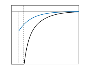
The numerically optimal bounds on $\langle w T \rangle$ are compared to the analytical bound (4.15) in figure 3(a). The former are zero until $ {\textit {R}}_E = 2147$, which differs from the energy stability limit reported by Goluskin (Reference Goluskin2015) due to the choice of horizontal period made in our numerical implementation. The inset (b) reveals that the optimal and analytical bounds appear to tend to the same asymptotic value as $ {\textit {R}} \to \infty$. Moreover, as evidenced by panel (c), they seem to do so at the same rate. This suggests that the only possible improvement to our analytical bound is in the coefficient of the $O( {\textit {R}}^{-(1/3)})$ correction, which for our numerically optimal bound is estimated to be $5.184 \pm 0.062$.

Figure 3. (a) Numerically optimal bounds $U_{n}$ computed with quinopt (black solid line), compared to the analytical bound $U_{a}$ (4.15) (blue solid line) and the improved uniform upper bound $\frac 12(\frac 12 + \frac {1}{\sqrt {3}})$ (dotted line). The inset (b) shows the ratio of the two R-dependent bounds. (c) Analytical (blue) and numerical (black) corrections to the uniform bound $\frac 12(\frac 12 + \frac {1}{\sqrt {3}})$, compensated by $ {\textit {R}}^{1/3}$. (d) Numerically optimal profiles $\phi '$ for $10^{3} \leq {\textit {R}} \leq 10^{9}$ (grey). Highlighted profiles for $ {\textit {R}} = 10^{5}$ (yellow), $ {\textit {R}} = 10^{7}$ (red) and $ {\textit {R}} = 10^{9}$ (brown) correspond to the circles in panels (a) and (c). (e) Balance parameters $a$ (blue solid line, optimal; blue dashed line, analytical) and $b$ (orange solid line, optimal; orange dashed line, analytical).

Figures 3(d) and 3(e) show the optimal profiles of $\phi '$ and the optimal balance parameters $a,b$ in the range of $ {\textit {R}}$ spanned by our computations. For large $ {\textit {R}}$, the optimal $\phi '$ are approximately piecewise linear, corroborating our analytical choice in (4.5a,b), and the optimal balance parameters behave like the analytical ones from § 4 (plotted with dashed lines). The main differences between the optimal and analytical $\phi '$ profiles are oscillations near the edge of the boundary layers and the fact that the two boundary layers of the optimal $\phi '$ have different widths. This suggests that a better prefactor for the $O( {\textit {R}}^{-(1/3)})$ term in our analytical bound could be obtained, at the expense of more complicated algebra, by considering boundary layers of different sizes.