


1 Introduction
The flow past a wingtip is a widely studied and modelled flow configuration due to its importance in both aeronautical and maritime applications. In aeronautical applications, hazardous flight conditions during take-off and landing at airports are encountered by smaller aircraft as their paths cross the wake of a larger plane. Strongly destabilizing moments on the smaller vehicle can result, at best, in passenger discomfort or, at worst, in irrecoverable loss of control (Spalart Reference Spalart1998). To ensure the safety of aircraft with similar flight paths, air-traffic regulations call for minimum following distances that depend on the size and weight of the leading as well as following aircraft. These distances are meant to allow sufficient time for the strongly vortical flow, forming off the wingtip, to weaken to a point where it no longer poses a hazard to the following aircraft. In light of ever-increasing air traffic, especially at major airport hubs, these impositions on the take-off and landing frequency are responsible for growing air-traffic congestion and require the use of fuel-inefficient and time-consuming holding patterns (Spalart Reference Spalart1998). Beyond aeronautical applications, manoeuvring maritime vessels shed wake vortices, generating a measurable footprint when stealth is desired (Wren Reference Wren1997). It thus seems prudent to investigate the dynamical and stability characteristics of the vortical wake structures, generated by the wingtip or other control surface to lay a theoretical foundation for the manipulation of their decay rates.
Despite the clear benefits from the hastened decay of these vortices, limited passive or active control research has been applied to practical configurations. There is an appreciable body of literature showing reasonable success in controlling wingtip vortices (Matalanis & Eaton Reference Matalanis and Eaton2007; Margaris & Gursul Reference Margaris and Gursul2010; Greenblatt Reference Greenblatt2012), but optimization is generally performed through tedious exploration of a large parameter space, after which the precise global optimum remains unknown. One way to help navigate this parameter space and to support control efforts is to determine unstable frequencies and wavelengths via a stability analysis.
Analyses of flow past a wingtip have thus far mainly concentrated on its two principal components in isolation: the shed trailing-line vortex and the airfoil wake. Regarding the former, the well-known Crow instability (Crow Reference Crow1970) results from the interaction of two counter-rotating vortices that shed from each wingtip and excite growing oscillations that result in the eventual breakup of the vortices into less hazardous vortex rings. It is a long-wavelength instability that can in turn be utilized as a control device by varying the load distribution along the wing, either by engaging the flaps and ailerons (Spalart Reference Spalart1998) or by rapidly actuating segmented Gurney flaps (Matalanis & Eaton Reference Matalanis and Eaton2007). These techniques, however, may result in accelerated structural fatigue due to the associated oscillatory loads.
Aside from the Crow instability, previous studies have also concentrated on isolated trailing vortex flows. Batchelor (Reference Batchelor1964), using a far-field approximation, derived an analytical expression that models these trailing vortices. This so-called Batchelor vortex has been the subject of several, initially parallel, stability analyses in both inviscid (Lessen, Singh & Paillet Reference Lessen, Singh and Paillet1974) and viscous (Lessen & Paillet Reference Lessen and Paillet1974; Khorrami Reference Khorrami1991; Mayer & Powell Reference Mayer and Powell1992; Fabre & Jacquin Reference Fabre and Jacquin2004) settings. These studies provided neutral stability curves for a large range of swirl numbers, Reynolds numbers and wavelengths. Initial studies showed that asymmetric disturbances opposing the flow direction resulted in instability for a moderate swirl parameter. For a swirl parameter larger than 1.5 the flow field was thought to be stable in the inviscid limit (Lessen et al. Reference Lessen, Singh and Paillet1974; Mayer & Powell Reference Mayer and Powell1992). However, Fabre & Jacquin (Reference Fabre and Jacquin2004) found that for very large but finite Reynolds numbers, viscous effects destabilize the flow for all values of swirl. Relaxing the parallel flow approximation, a bi-global parabolized stability analysis on the developing Batchelor vortex was conducted using spectral element techniques (Broadhurst Reference Broadhurst2006) and higher-order finite-difference methods (Paredes, Rodriguez & Theofilis Reference Paredes, Rodriguez and Theofilis2013). Heaton, Nichols & Schmid (Reference Heaton, Nichols and Schmid2009) discretized both the radial and streamwise directions for a global approach, while also allowing for instabilities in both space and time. These analyses showed that the global spectrum had similar structure to the parallel case, corroborating the weakly non-parallel base-flow assumption in earlier studies. Despite this far-field approximation, there has been reasonable agreement between the stability results of a fit Batchelor vortex and experimentally obtained modes of a trailing vortex (Edstrand et al. Reference Edstrand, Davis, Schmid, Taira and Cattafesta2016).
While the aforementioned efforts provide valuable insights into the intrinsic instabilities and their streamwise development, due to the far-field approximation of the Batchelor vortex, the results are generally of limited use for control design as the instabilities arise far from the wing surface and are thus difficult to manipulate by common wing-mounted control devices. In the so-called intermediate field (figure 1), the shed vortex shows a marked asymmetry, the vortex sheet is not fully rolled up and the wake of the wing constitutes an important component of the base flow. Consequently, the stability characteristics of the full base flow are expected to differ from the results obtained for the Batchelor vortex.

Figure 1. A NACA0012 wing with the identified near, intermediate and far-field regions and flow fields. The near field is defined as the region of vortex development along the airfoil surface. The coordinate system is indicated with the origin at the trailing edge of the wing tip, where
 $x$
denotes the streamwise direction,
$x$
denotes the streamwise direction,
 $z$
denotes the spanwise direction and
$z$
denotes the spanwise direction and
 $y$
completes the right-handed coordinate system. The green box designates the region of interest for our stability analysis, ranging from
$y$
completes the right-handed coordinate system. The green box designates the region of interest for our stability analysis, ranging from
 $x=0$
to 15. Note that although
$x=0$
to 15. Note that although
 $x=0$
is along the trailing edge, the green box does not reside directly along the trailing edge for clarity.
$x=0$
is along the trailing edge, the green box does not reside directly along the trailing edge for clarity.
Aside from the asymptotic trailing vortex, other stability analyses have considered the wake of a two-dimensional airfoil using empirical fits (Mattingly & Criminale Reference Mattingly and Criminale1972), double Blasius profiles (Papageorgiou & Smith Reference Papageorgiou and Smith1989) or Falkner–Skan profiles (Woodley & Peake Reference Woodley and Peake1997) as models for the base flow. The empirical profiles performed rather well in a stability analysis of the downstream domain, but the results deteriorated in the vicinity of the trailing edge. Blasius and Falkner–Skan profiles provided good agreement with experimental data (Sato & Kuriki Reference Sato and Kuriki1961) near the trailing edge. Woodley & Peake (Reference Woodley and Peake1997) introduced a critical Reynolds number, which generally depends on the geometry and the induced adverse pressure gradient; above this value, the onset of global linear instabilities is observed.
In contrast to these previous studies, the near wake behind a three-dimensional wing contains spanwise velocity components, and the presence of the vortex developing off the wingtip further complicates the base-flow velocity field. For this reason, even though the instabilities of the wake may dominate the overall flow behaviour under certain circumstances, only a global analysis of the composite wake–vortex flow field can provide information about the presence of pertinent instability mechanisms and their relative importance. For completeness, we compare the global analysis against the canonical wake and vortex flows in § 4.5. Furthermore, with potential applications to receptivity, we approximate the dispersion relationship through a second-order Taylor series expansion in a so-called wavepacket analysis (Trefethen Reference Trefethen2005; Obrist & Schmid Reference Obrist and Schmid2010). This analysis may provide insight into the way the asymmetry of the base flow affects the receptivity of the flow field to free-stream disturbances with relatively low computational cost.
A schematic illustrating the development of the trailing vortex is provided in figure 1, in which three regions are identified: the near-field development of the tip vortex, the intermediate field involving the self-similar roll up and interaction with the wake and the far-field region in which the vortex assumes an axisymmetric shape. Our primary interest lies in the intermediate field, indicated by the green box in figure 1, where the trailing vortex is asymmetric and prone to a strong wake interaction. In this regime, the flow field is dominated by strong streamwise convection, with streamwise diffusion causing only a weak non-parallelism in the base flow and a self-similar vortex roll up (Devenport et al. Reference Devenport, Rife, Liapis and Follin1996). Based on these observations, the present study adopts a parallel-flow assumption in the streamwise direction as we expect the stability characteristics to show only a minor dependence on the slow streamwise variation of the base flow. For the cross plane at each streamwise location, a bi-global stability analysis (Theofilis Reference Theofilis, Joslin and Miller2009, Reference Theofilis2011) is performed. For more accurate results, a bi-global parabolized analysis (Herbert Reference Herbert1997) that takes into account slow streamwise variation should be utilized. However, for the parabolized analysis, the parallel approximation is the initial condition and therefore the parallel assumption is a necessary first step prior to moving forward to a parabolized analysis. Therefore, this paper provides pertinent insight into future analyses that are parabolized in nature.
In the present study, we consider a low chord-based Reynolds number of
 $Re_{c}=1000$
, such that the flow is laminar and fundamental in nature without the complications that emerge from the treatment of turbulent stresses and their effect on the stability analysis (Viola et al.
Reference Viola, Iungo, Camarri, Porté-Agel and Gallaire2014). This regime is also relevant for aerodynamic applications related to biological flight and micro air vehicles. The wings seen in those fields of study are characterized by their low-aspect-ratio planforms whose aerodynamic characteristics are strongly influenced by tip vortices and three-dimensional effects (Torres & Mueller Reference Torres and Mueller2004; Taira & Colonius Reference Taira and Colonius2009). Thus the present stability analysis not only uncovers insights for potential vortex–wake mitigation but also provides basic knowledge on tip-effect for low Reynolds number aerodynamics.
$Re_{c}=1000$
, such that the flow is laminar and fundamental in nature without the complications that emerge from the treatment of turbulent stresses and their effect on the stability analysis (Viola et al.
Reference Viola, Iungo, Camarri, Porté-Agel and Gallaire2014). This regime is also relevant for aerodynamic applications related to biological flight and micro air vehicles. The wings seen in those fields of study are characterized by their low-aspect-ratio planforms whose aerodynamic characteristics are strongly influenced by tip vortices and three-dimensional effects (Torres & Mueller Reference Torres and Mueller2004; Taira & Colonius Reference Taira and Colonius2009). Thus the present stability analysis not only uncovers insights for potential vortex–wake mitigation but also provides basic knowledge on tip-effect for low Reynolds number aerodynamics.
The article is structured as follows. We first present the base flow, together with the computational approach and the employed numerical methods for the stability analysis. We then perform a temporal stability analysis, concentrating on the discrete, continuous and wavepacket pseudomodal structures of the spectrum. These results are then contrasted with a spatial linear analysis, and links between these two types of analysis are established. In the final section, we summarize our results and offer conclusions.
2 Computational approach and validation
2.1 Base flow
The base flow behind a wing is a complex flow field for which no analytical solution exists; therefore, the base flow is determined numerically. We utilize direct numerical simulation to compute the flow around a NACA0012 profile with a flat wingtip positioned at an angle of attack of
 $5^{\circ }$
. The chord Reynolds number is fixed at
$5^{\circ }$
. The chord Reynolds number is fixed at
 $Re_{c}=1000$
with a half-span
$Re_{c}=1000$
with a half-span
 $b/2=1.25$
and a chord
$b/2=1.25$
and a chord
 $c=1$
, allowing for all spatial coordinates to correspond to their non-dimensional values based on the chord length. In the transverse (
$c=1$
, allowing for all spatial coordinates to correspond to their non-dimensional values based on the chord length. In the transverse (
 $y$
) direction, the computational domain extends over the interval
$y$
) direction, the computational domain extends over the interval
 $y\in [-15,\,15]$
, while in the spanwise (
$y\in [-15,\,15]$
, while in the spanwise (
 $z$
) direction we take
$z$
) direction we take
 $z\in [-1.25,\,14.375]$
. The streamwise direction extends in a semi-circular arc with a radius of 15 and progresses downstream 15 chords, discretized by a C-grid.
$z\in [-1.25,\,14.375]$
. The streamwise direction extends in a semi-circular arc with a radius of 15 and progresses downstream 15 chords, discretized by a C-grid.
An incompressible, finite-volume flow solver, Cliff (CharLES package), developed by Cascade Technologies (Ham & Iaccarino Reference Ham and Iaccarino2004; Ham, Mattsson & Iaccarino Reference Ham, Mattsson and Iaccarino2006), is used, which is second-order accurate in both time and space. The boundary conditions at the inlet are prescribed with
 $(U,V,W)=(1,0,0)$
, and at the outlet a convective outflow boundary condition is employed. In the far field and on the symmetry plane, we impose free-slip boundary conditions.
$(U,V,W)=(1,0,0)$
, and at the outlet a convective outflow boundary condition is employed. In the far field and on the symmetry plane, we impose free-slip boundary conditions.
The flow around the wing is simulated with approximately 3.5 million elements. The spatial field is discretized on a hybrid mesh, where the boundary layer and wake regions are covered by a structured grid, while the far field outside this region is computed on an unstructured grid consisting of tetrahedral elements. To ensure the grid is sufficient, we locally increase the number of elements in the wake by approximately 2.1 million in the wake region, showing that the refined case recreated the same flow field that contains minimal differences. The computational domain is chosen such that the cross-section of the wing contains a blockage ratio of less than 0.5 %, indicating that the domain size is sufficiently large. These results provide us with confidence that the base flow accurately captures the trailing-line vortex in free space.
The simulation ran until it reached a steady-state base flow, shown in figure 2. The blue iso-surface visualizes the trailing vortex with the
 $Q$
-criterion (Jeong & Hussain Reference Jeong and Hussain1995). As shown, the vortex core evolves smoothly downstream, with the radius slightly diminishing in size with downstream progression due to viscous diffusion. A contour slice shows the streamwise velocity deficit in the wake of the airfoil at
$Q$
-criterion (Jeong & Hussain Reference Jeong and Hussain1995). As shown, the vortex core evolves smoothly downstream, with the radius slightly diminishing in size with downstream progression due to viscous diffusion. A contour slice shows the streamwise velocity deficit in the wake of the airfoil at
 $x=3$
, i.e. the plane to be examined in this paper. Our study focuses on this plane because flow at this location is influenced by both the wake and the trailing vortex allowing us to gain insight into both wake and trailing vortex instabilities.
$x=3$
, i.e. the plane to be examined in this paper. Our study focuses on this plane because flow at this location is influenced by both the wake and the trailing vortex allowing us to gain insight into both wake and trailing vortex instabilities.

Figure 2. The base flow at
 $Re_{c}=1000$
, visualized with blue iso-surfaces, showing the
$Re_{c}=1000$
, visualized with blue iso-surfaces, showing the
 $Q$
-criterion (
$Q$
-criterion (
 $Q=0.25$
). The dark grey region corresponds to the wing location. The contour slice of the streamwise velocity at
$Q=0.25$
). The dark grey region corresponds to the wing location. The contour slice of the streamwise velocity at
 $x=3$
illustrates the streamwise velocity deficit in the wake region, while the
$x=3$
illustrates the streamwise velocity deficit in the wake region, while the
 $Q$
-criterion visualizes the structure of the trailing vortex.
$Q$
-criterion visualizes the structure of the trailing vortex.
The downstream development of the streamwise (
 $U$
), transverse (
$U$
), transverse (
 $V$
) and spanwise (
$V$
) and spanwise (
 $W$
) velocity profiles are shown in figure 3 at
$W$
) velocity profiles are shown in figure 3 at
 $z=-1.25$
and
$z=-1.25$
and
 $-0.25$
(i.e. midspan of the wing and 80 % span, respectively). At the midspan of the wing (corresponding to
$-0.25$
(i.e. midspan of the wing and 80 % span, respectively). At the midspan of the wing (corresponding to
 $z=-1.25$
, figure 3
a), a streamwise velocity deficit is observed near the trailing edge. This deficit advects downward, indicated by the dash-dotted line of the minimum velocity, due to the downwash caused by the induced negative transverse velocity. At
$z=-1.25$
, figure 3
a), a streamwise velocity deficit is observed near the trailing edge. This deficit advects downward, indicated by the dash-dotted line of the minimum velocity, due to the downwash caused by the induced negative transverse velocity. At
 $z=-0.25$
(figure 3
b), the higher level of transverse velocity advects the streamwise velocity deficit farther upstream, causing the wake to descend more rapidly. The spanwise velocity,
$z=-0.25$
(figure 3
b), the higher level of transverse velocity advects the streamwise velocity deficit farther upstream, causing the wake to descend more rapidly. The spanwise velocity,
 $W$
, is zero at the midspan location, but increases approximately to the level of the transverse velocity at
$W$
, is zero at the midspan location, but increases approximately to the level of the transverse velocity at
 $z=-0.25$
. At
$z=-0.25$
. At
 $x=3$
, the effect of the wake is significant, but not so overwhelming as to overshadow the effect of the developing vortex on the stability analysis. Hence, we select
$x=3$
, the effect of the wake is significant, but not so overwhelming as to overshadow the effect of the developing vortex on the stability analysis. Hence, we select
 $x=3$
as a representative location to examine the combined efforts from the wake and trailing vortex onto the stability of the flow.
$x=3$
as a representative location to examine the combined efforts from the wake and trailing vortex onto the stability of the flow.

Figure 3. Streamwise (
 $U$
, dashed line), transverse (
$U$
, dashed line), transverse (
 $V$
, solid line) and spanwise (
$V$
, solid line) and spanwise (
 $W$
, dotted line) velocities (
$W$
, dotted line) velocities (
 $V$
and
$V$
and
 $W$
are scaled up by a factor of 5 for graphical clarity) of the wake of the wing at
$W$
are scaled up by a factor of 5 for graphical clarity) of the wake of the wing at
 $z=-1.25$
(a) and
$z=-1.25$
(a) and
 $z=-0.25$
(b) with downstream progression from
$z=-0.25$
(b) with downstream progression from
 $x=0$
to 5. The dash-dotted line with the solid-dot markers shows the point of minimum axial velocity deficit in the wake. The
$x=0$
to 5. The dash-dotted line with the solid-dot markers shows the point of minimum axial velocity deficit in the wake. The
 $x$
-locations are
$x$
-locations are
 $x=0,1.5,3$
and 4.5.
$x=0,1.5,3$
and 4.5.
2.2 Stability analysis approach and validation
We examine the modal behaviour of small perturbations about the given base flow. Following standard linear stability analysis formulation, the state variable can be decomposed into the steady base flow and an unsteady disturbance as
 $$\begin{eqnarray}\displaystyle \tilde{\boldsymbol{q}}(x,y,z,t)=Q(x,y,z)+\unicode[STIX]{x1D716}\hat{q}(x,y,z,t). & & \displaystyle\end{eqnarray}$$
Here,
 $\tilde{\boldsymbol{q}}=(\tilde{u} ,\,\tilde{v},\,\tilde{w},\,\tilde{p})^{\text{T}}$
denotes the state vector,
$\tilde{\boldsymbol{q}}=(\tilde{u} ,\,\tilde{v},\,\tilde{w},\,\tilde{p})^{\text{T}}$
denotes the state vector,
 $Q=(U,\,V,\,W,\,P)^{\text{T}}$
is the known steady base flow,
$Q=(U,\,V,\,W,\,P)^{\text{T}}$
is the known steady base flow,
 $\hat{q}=(\hat{u} ,\,\hat{v},\,{\hat{w}},\,\hat{p})^{\text{T}}$
represents the disturbance and
$\hat{q}=(\hat{u} ,\,\hat{v},\,{\hat{w}},\,\hat{p})^{\text{T}}$
represents the disturbance and
 $\unicode[STIX]{x1D716}$
stands for a small disturbance amplitude. By only considering small disturbances, we neglect the nonlinear,
$\unicode[STIX]{x1D716}$
stands for a small disturbance amplitude. By only considering small disturbances, we neglect the nonlinear,
 $O(\unicode[STIX]{x1D716}^{2})$
terms in the incompressible Navier–Stokes equations, which in turn results in the linearized disturbance equations (Schmid & Henningson Reference Schmid and Henningson2001). In the intermediate region behind the airfoil, the slow process of viscous diffusion relative to streamwise convection produces a quasi-parallel flow, with streamwise gradients being less than 2.75 % of the transverse gradients. This quasi-parallel assumption on streamwise variations of the base flow leads to the disturbance equations with constant coefficients in the streamwise direction and permits wave-like disturbance solutions of the form
$O(\unicode[STIX]{x1D716}^{2})$
terms in the incompressible Navier–Stokes equations, which in turn results in the linearized disturbance equations (Schmid & Henningson Reference Schmid and Henningson2001). In the intermediate region behind the airfoil, the slow process of viscous diffusion relative to streamwise convection produces a quasi-parallel flow, with streamwise gradients being less than 2.75 % of the transverse gradients. This quasi-parallel assumption on streamwise variations of the base flow leads to the disturbance equations with constant coefficients in the streamwise direction and permits wave-like disturbance solutions of the form
 $$\begin{eqnarray}\displaystyle \hat{q}(x,y,z,t)=q(y,z)\exp (\text{i}\unicode[STIX]{x1D6FC}x-\text{i}\unicode[STIX]{x1D714}t). & & \displaystyle\end{eqnarray}$$
In the above expression,
 $q(y,z)$
denotes the shape function, and the argument in the exponent of (2.2) is the phase function, where
$q(y,z)$
denotes the shape function, and the argument in the exponent of (2.2) is the phase function, where
 $\unicode[STIX]{x1D6FC}$
and
$\unicode[STIX]{x1D6FC}$
and
 $\unicode[STIX]{x1D714}$
represent the streamwise wavenumber and radian frequency, respectively. Substitution of (2.2) into the linearized disturbance equations results in a generalized eigenvalue problem. The specific form of the eigenvalue problem depends on the type of stability analysis. For a temporal stability analysis, we assume growth/decay in time and allow for a complex frequency
$\unicode[STIX]{x1D714}$
represent the streamwise wavenumber and radian frequency, respectively. Substitution of (2.2) into the linearized disturbance equations results in a generalized eigenvalue problem. The specific form of the eigenvalue problem depends on the type of stability analysis. For a temporal stability analysis, we assume growth/decay in time and allow for a complex frequency
 $\unicode[STIX]{x1D714}=\unicode[STIX]{x1D714}_{r}+\text{i}\unicode[STIX]{x1D714}_{i}$
, with
$\unicode[STIX]{x1D714}=\unicode[STIX]{x1D714}_{r}+\text{i}\unicode[STIX]{x1D714}_{i}$
, with
 $\unicode[STIX]{x1D714}_{i}>0$
denoting exponential growth at the radian frequency
$\unicode[STIX]{x1D714}_{i}>0$
denoting exponential growth at the radian frequency
 $\unicode[STIX]{x1D714}_{r}$
. The associated eigenvalue problem reads
$\unicode[STIX]{x1D714}_{r}$
. The associated eigenvalue problem reads
 ${\mathcal{A}}_{T}\boldsymbol{q}=\unicode[STIX]{x1D714}{\mathcal{B}}_{T}\boldsymbol{q}$
where
${\mathcal{A}}_{T}\boldsymbol{q}=\unicode[STIX]{x1D714}{\mathcal{B}}_{T}\boldsymbol{q}$
where
 ${\mathcal{A}}_{T}$
and
${\mathcal{A}}_{T}$
and
 ${\mathcal{B}}_{T}$
are defined in appendix A. Conversely, for a spatial stability analysis, the streamwise wavenumber
${\mathcal{B}}_{T}$
are defined in appendix A. Conversely, for a spatial stability analysis, the streamwise wavenumber
 $\unicode[STIX]{x1D6FC}$
represents the complex eigenvalue
$\unicode[STIX]{x1D6FC}$
represents the complex eigenvalue
 $\unicode[STIX]{x1D6FC}=\unicode[STIX]{x1D6FC}_{r}+\text{i}\unicode[STIX]{x1D6FC}_{i}$
with
$\unicode[STIX]{x1D6FC}=\unicode[STIX]{x1D6FC}_{r}+\text{i}\unicode[STIX]{x1D6FC}_{i}$
with
 $\unicode[STIX]{x1D6FC}_{i}<0$
indicating spatial exponential growth. The corresponding eigenvalue problem is nonlinear in the eigenvalue
$\unicode[STIX]{x1D6FC}_{i}<0$
indicating spatial exponential growth. The corresponding eigenvalue problem is nonlinear in the eigenvalue
 $\unicode[STIX]{x1D6FC},$
but can be recast into an equivalent linear problem
$\unicode[STIX]{x1D6FC},$
but can be recast into an equivalent linear problem
 ${\mathcal{A}}_{S}\boldsymbol{q}_{S}=\unicode[STIX]{x1D6FC}{\mathcal{B}}_{S}\boldsymbol{q}_{S}$
via a companion matrix technique (Tisseur & Meerbergen Reference Tisseur and Meerbergen2001). The operators
${\mathcal{A}}_{S}\boldsymbol{q}_{S}=\unicode[STIX]{x1D6FC}{\mathcal{B}}_{S}\boldsymbol{q}_{S}$
via a companion matrix technique (Tisseur & Meerbergen Reference Tisseur and Meerbergen2001). The operators
 ${\mathcal{A}}_{S}$
and
${\mathcal{A}}_{S}$
and
 ${\mathcal{B}}_{S}$
are also defined in appendix A.
${\mathcal{B}}_{S}$
are also defined in appendix A.
The spatial discretization of the respective stability matrices
 ${\mathcal{A}}$
and
${\mathcal{A}}$
and
 ${\mathcal{B}}$
is performed using the Chebyshev-based spectral collocation method (Kopriva Reference Kopriva2009). The Chebyshev Gauss–Lobatto points
${\mathcal{B}}$
is performed using the Chebyshev-based spectral collocation method (Kopriva Reference Kopriva2009). The Chebyshev Gauss–Lobatto points
 $\unicode[STIX]{x1D702}_{j}$
are mapped onto the transverse coordinate direction
$\unicode[STIX]{x1D702}_{j}$
are mapped onto the transverse coordinate direction
 $y$
using (Hein & Theofilis Reference Hein and Theofilis2004)
$y$
using (Hein & Theofilis Reference Hein and Theofilis2004)
 $$\begin{eqnarray}\displaystyle y_{j}=g(\unicode[STIX]{x1D702}_{j};\unicode[STIX]{x1D705},y_{\infty })=y_{\infty }\frac{\tan \left(\displaystyle \frac{\unicode[STIX]{x1D705}\unicode[STIX]{x03C0}\unicode[STIX]{x1D702}_{j}}{2}\right)}{\tan \left(\displaystyle \frac{\unicode[STIX]{x1D705}\unicode[STIX]{x03C0}}{2}\right)},\quad j=0,1,\ldots ,N_{y}, & & \displaystyle\end{eqnarray}$$
where
 $y_{\infty }$
denotes the largest far-field
$y_{\infty }$
denotes the largest far-field
 $y$
-value noted below, and the parameter
$y$
-value noted below, and the parameter
 $\unicode[STIX]{x1D705}$
adjusts the spread of the points about
$\unicode[STIX]{x1D705}$
adjusts the spread of the points about
 $y=0$
. When examining the discrete branches that are isolated in the vortex regions, we use a value of
$y=0$
. When examining the discrete branches that are isolated in the vortex regions, we use a value of
 $\unicode[STIX]{x1D705}=0.96$
. In contrast, when analysing the continuous branch, we require a larger number of points in the free stream, and thus relax the parameter to
$\unicode[STIX]{x1D705}=0.96$
. In contrast, when analysing the continuous branch, we require a larger number of points in the free stream, and thus relax the parameter to
 $\unicode[STIX]{x1D705}=0.85$
, yielding more gradual stretching of the grid.
$\unicode[STIX]{x1D705}=0.85$
, yielding more gradual stretching of the grid.
In the spanwise coordinate direction with
 $z\in [-1.25,14.375]$
, two nested mappings are utilized. First, equation (2.3) is used to map
$z\in [-1.25,14.375]$
, two nested mappings are utilized. First, equation (2.3) is used to map
 $\unicode[STIX]{x1D701}_{j}\rightarrow \unicode[STIX]{x1D701}_{j}^{\ast }$
, where
$\unicode[STIX]{x1D701}_{j}\rightarrow \unicode[STIX]{x1D701}_{j}^{\ast }$
, where
 $\unicode[STIX]{x1D701}_{j}$
denotes the Gauss–Lobatto points in the
$\unicode[STIX]{x1D701}_{j}$
denotes the Gauss–Lobatto points in the
 $z$
-direction, and
$z$
-direction, and
 $\unicode[STIX]{x1D701}_{j}^{\ast }$
are the mapped points per (2.3). Throughout this study,
$\unicode[STIX]{x1D701}_{j}^{\ast }$
are the mapped points per (2.3). Throughout this study,
 $\unicode[STIX]{x1D705}$
in the
$\unicode[STIX]{x1D705}$
in the
 $z$
-direction is set to be equal to the value used in the
$z$
-direction is set to be equal to the value used in the
 $y$
-direction. We maintain the far-field value to be
$y$
-direction. We maintain the far-field value to be
 $\unicode[STIX]{x1D701}_{\infty }^{\ast }=1$
to preserve the scale on
$\unicode[STIX]{x1D701}_{\infty }^{\ast }=1$
to preserve the scale on
 $\unicode[STIX]{x1D701}^{\ast }\in [-1,1]$
. With the points reclustered about the centre, we then apply the second mapping from
$\unicode[STIX]{x1D701}^{\ast }\in [-1,1]$
. With the points reclustered about the centre, we then apply the second mapping from
 $\unicode[STIX]{x1D701}^{\ast }$
to
$\unicode[STIX]{x1D701}^{\ast }$
to
 $z\in [-1.25,14.375]$
using a rational function (Hanifi, Schmid & Henningson Reference Hanifi, Schmid and Henningson1996)
$z\in [-1.25,14.375]$
using a rational function (Hanifi, Schmid & Henningson Reference Hanifi, Schmid and Henningson1996)
 $$\begin{eqnarray}\displaystyle z_{j}=h(\unicode[STIX]{x1D701}_{j}^{\ast };z_{min},z_{mid},z_{\infty })=z_{min}+a\frac{1+\unicode[STIX]{x1D701}_{j}^{\ast }}{b-\unicode[STIX]{x1D701}_{j}^{\ast }},\quad j=0,1,\ldots ,N_{z}, & & \displaystyle\end{eqnarray}$$
with
 $$\begin{eqnarray}\displaystyle a=\frac{z_{mid}z_{\infty }}{z_{\infty }-2z_{mid}},\quad b=1+\frac{2a}{z_{\infty }}. & & \displaystyle\end{eqnarray}$$
We choose
 $z_{min}=-1.25$
,
$z_{min}=-1.25$
,
 $z_{mid}=1.25$
and
$z_{mid}=1.25$
and
 $z_{\infty }=15.625$
. The above expression distributes half the mapped collocation points to cluster below and above
$z_{\infty }=15.625$
. The above expression distributes half the mapped collocation points to cluster below and above
 $z_{mid}$
prior to translating the data by
$z_{mid}$
prior to translating the data by
 $z_{min}$
.
$z_{min}$
.
Stability analyses show relative insensitivity of the leading eigenvalue to the choice of domain size owing to the exponential decay of its eigenfunction outside the shear layer. For this reason, final computations are performed on the domain of
 $y\in [-10,10]$
and
$y\in [-10,10]$
and
 $z\in [-1.25,10]$
in order to achieve satisfactory resolution within the vortex and wake regions. The discretized eigenvalue problem is solved using the implicitly restarted Arnoldi method with the shift-and-invert technique implemented in ARPACK (Lehoucq, Sorensen & Yang Reference Lehoucq, Sorensen and Yang1996).
$z\in [-1.25,10]$
in order to achieve satisfactory resolution within the vortex and wake regions. The discretized eigenvalue problem is solved using the implicitly restarted Arnoldi method with the shift-and-invert technique implemented in ARPACK (Lehoucq, Sorensen & Yang Reference Lehoucq, Sorensen and Yang1996).
Table 1. Validation of the present temporal and spatial analyses with duct flow (Theofilis, Duck & Owen Reference Theofilis, Duck and Owen2004) and the Batchelor vortex (Paredes Reference Paredes2014), respectively. Shown are the least stable eigenvalues with convergence. Also included (rightmost column) are results of our temporal stability analysis of the flow past a wingtip for
 $\unicode[STIX]{x1D6FC}=5.5$
at
$\unicode[STIX]{x1D6FC}=5.5$
at
 $Re_{c}=1000$
, demonstrating convergence of the converged least stable eigenvalue as the grid is refined.
$Re_{c}=1000$
, demonstrating convergence of the converged least stable eigenvalue as the grid is refined.

Our bi-global stability code is validated against stability analyses of two-dimensional channel flow (Theofilis et al.
Reference Theofilis, Duck and Owen2004; Paredes Reference Paredes2014) and the Batchelor vortex (Fabre & Jacquin Reference Fabre and Jacquin2004; Paredes Reference Paredes2014). The results of these validations are displayed in table 1. For the present analysis, convergence towards a relative error of
 $10^{-4}$
is achieved for a resolution of
$10^{-4}$
is achieved for a resolution of
 $N_{z}\times N_{y}=60\times 60$
. Therefore, for cases that require a large number of eigenvalue problems to be solved, we employ
$N_{z}\times N_{y}=60\times 60$
. Therefore, for cases that require a large number of eigenvalue problems to be solved, we employ
 $N_{y}\times N_{z}=60\times 60$
, and for single case studies, we increase the number to
$N_{y}\times N_{z}=60\times 60$
, and for single case studies, we increase the number to
 $N_{y}\times N_{z}=80\times 80$
for more accurate results.
$N_{y}\times N_{z}=80\times 80$
for more accurate results.
3 Temporal bi-global stability analysis
We begin with a series of temporal analyses and parametrically sweep the streamwise wavenumber
 $\unicode[STIX]{x1D6FC}$
to determine the most unstable condition (in our case, for
$\unicode[STIX]{x1D6FC}$
to determine the most unstable condition (in our case, for
 $\unicode[STIX]{x1D6FC}=5.5$
for a chord-based Reynolds number of
$\unicode[STIX]{x1D6FC}=5.5$
for a chord-based Reynolds number of
 $Re_{c}=1000$
). We then focus on this streamwise wavenumber and present a detailed analysis of the bi-global spectrum, identifying and examining the discrete branches, the continuous part (free stream) and the region of the complex
$Re_{c}=1000$
). We then focus on this streamwise wavenumber and present a detailed analysis of the bi-global spectrum, identifying and examining the discrete branches, the continuous part (free stream) and the region of the complex
 $\unicode[STIX]{x1D714}$
-plane that is dominated by wavepacket eigenfunctions (see Trefethen Reference Trefethen2005; Obrist & Schmid Reference Obrist and Schmid2008, Reference Obrist and Schmid2010). Each part of the bi-global spectrum will be categorized and, where available, supported by analytical or approximate computational results and scalings.
$\unicode[STIX]{x1D714}$
-plane that is dominated by wavepacket eigenfunctions (see Trefethen Reference Trefethen2005; Obrist & Schmid Reference Obrist and Schmid2008, Reference Obrist and Schmid2010). Each part of the bi-global spectrum will be categorized and, where available, supported by analytical or approximate computational results and scalings.
3.1 Parametric dependence on the streamwise wavenumber
Starting with a base-flow profile extracted at the streamwise position of
 $x=3$
, we solve the bi-global temporal stability problem and vary the streamwise wavenumber from
$x=3$
, we solve the bi-global temporal stability problem and vary the streamwise wavenumber from
 $\unicode[STIX]{x1D6FC}=2$
to 6.5 in increments of
$\unicode[STIX]{x1D6FC}=2$
to 6.5 in increments of
 $\unicode[STIX]{x0394}\unicode[STIX]{x1D6FC}=0.5$
. Recall that the
$\unicode[STIX]{x0394}\unicode[STIX]{x1D6FC}=0.5$
. Recall that the
 $x=3$
location was chosen to examine both wake and tip vortex influences. The results are shown in figure 4. Three particular eigenvalues, representing a specific type of instabilities (see more details in § 3.3), are tracked: the first is termed the ‘principal wake instability’, the second eigenvalue is linked to a ‘vortex instability’ and the third, labelled ‘wake instability’, displays features consistent with a higher-order wake mode. The principal wake instability remains the primary instability throughout the range of
$x=3$
location was chosen to examine both wake and tip vortex influences. The results are shown in figure 4. Three particular eigenvalues, representing a specific type of instabilities (see more details in § 3.3), are tracked: the first is termed the ‘principal wake instability’, the second eigenvalue is linked to a ‘vortex instability’ and the third, labelled ‘wake instability’, displays features consistent with a higher-order wake mode. The principal wake instability remains the primary instability throughout the range of
 $\unicode[STIX]{x1D6FC}$
examined, while the relative strength of the wake and vortex instabilities are dependent on the streamwise wavenumber. For low-wavenumber disturbances (i.e. large wavelengths), the vortex instability grows more rapidly than the wake instability.
$\unicode[STIX]{x1D6FC}$
examined, while the relative strength of the wake and vortex instabilities are dependent on the streamwise wavenumber. For low-wavenumber disturbances (i.e. large wavelengths), the vortex instability grows more rapidly than the wake instability.

Figure 4. Temporal growth rate,
 $\unicode[STIX]{x1D714}_{i}$
, at
$\unicode[STIX]{x1D714}_{i}$
, at
 $x=3$
with varying streamwise wavenumber
$x=3$
with varying streamwise wavenumber
 $\unicode[STIX]{x1D6FC}$
, with
$\unicode[STIX]{x1D6FC}$
, with
 $N_{z}=N_{y}=60$
. The three instabilities are labelled as the principal wake instability, wake instability and vortex instability, according to their modal features. The dashed line indicates the wavenumber that we examine throughout the temporal analysis.
$N_{z}=N_{y}=60$
. The three instabilities are labelled as the principal wake instability, wake instability and vortex instability, according to their modal features. The dashed line indicates the wavenumber that we examine throughout the temporal analysis.
The maximum growth rate of the principal wake instability is
 $\unicode[STIX]{x1D714}_{i}\approx 0.34$
, which is achieved at a streamwise wavenumber of
$\unicode[STIX]{x1D714}_{i}\approx 0.34$
, which is achieved at a streamwise wavenumber of
 $\unicode[STIX]{x1D6FC}=5.5$
. At this wavenumber, both the wake and vortex instabilities show a growth rate of
$\unicode[STIX]{x1D6FC}=5.5$
. At this wavenumber, both the wake and vortex instabilities show a growth rate of
 $\unicode[STIX]{x1D714}_{i}\approx 0.18$
and
$\unicode[STIX]{x1D714}_{i}\approx 0.18$
and
 $\unicode[STIX]{x1D714}_{i}\approx 0.14$
, respectively, suggesting a balance between the vortex instability and the wake instability. With the wavenumber fixed at
$\unicode[STIX]{x1D714}_{i}\approx 0.14$
, respectively, suggesting a balance between the vortex instability and the wake instability. With the wavenumber fixed at
 $\unicode[STIX]{x1D6FC}=5.5$
, we now present the bi-global spectrum and analyse the associated modes in detail.
$\unicode[STIX]{x1D6FC}=5.5$
, we now present the bi-global spectrum and analyse the associated modes in detail.
3.2 The temporal bi-global spectrum – an overview
For a streamwise wavenumber of
 $\unicode[STIX]{x1D6FC}=5.5$
and a chord-based Reynolds number of
$\unicode[STIX]{x1D6FC}=5.5$
and a chord-based Reynolds number of
 $Re_{c}=1000$
, the temporal eigenvalue spectrum is displayed in the complex
$Re_{c}=1000$
, the temporal eigenvalue spectrum is displayed in the complex
 $\unicode[STIX]{x1D714}$
-plane in figure 5. The unstable half-plane
$\unicode[STIX]{x1D714}$
-plane in figure 5. The unstable half-plane
 $\unicode[STIX]{x1D714}_{i}>0$
is shaded in grey; instabilities, if any, lie in this upper half-plane. The quantitative values of these growth rates,
$\unicode[STIX]{x1D714}_{i}>0$
is shaded in grey; instabilities, if any, lie in this upper half-plane. The quantitative values of these growth rates,
 $\unicode[STIX]{x1D714}_{i}$
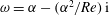
, are approximate due to the steady-state nature of the base flow, implying the discrete branches may shift upward or downward in figure 5 (Sipp & Lebedev Reference Sipp and Lebedev2007). Despite this, however, we retain confidence in the relative levels and qualitative structure of these modes. Dividing
$\unicode[STIX]{x1D714}_{i}$
, are approximate due to the steady-state nature of the base flow, implying the discrete branches may shift upward or downward in figure 5 (Sipp & Lebedev Reference Sipp and Lebedev2007). Despite this, however, we retain confidence in the relative levels and qualitative structure of these modes. Dividing
 $\unicode[STIX]{x1D714}_{r}$
by the wavenumber
$\unicode[STIX]{x1D714}_{r}$
by the wavenumber
 $\unicode[STIX]{x1D6FC}$
yields the streamwise phase speed, i.e. the speed at which the associated modes travel. Invoking a critical-layer argument (Schmid & Henningson Reference Schmid and Henningson2001), this speed generally relates directly to the local speed of the base flow, which implies that the disturbances with
$\unicode[STIX]{x1D6FC}$
yields the streamwise phase speed, i.e. the speed at which the associated modes travel. Invoking a critical-layer argument (Schmid & Henningson Reference Schmid and Henningson2001), this speed generally relates directly to the local speed of the base flow, which implies that the disturbances with
 $\unicode[STIX]{x1D714}_{r}<\unicode[STIX]{x1D6FC}$
are generally confined to regions of velocity deficit.
$\unicode[STIX]{x1D714}_{r}<\unicode[STIX]{x1D6FC}$
are generally confined to regions of velocity deficit.
The bi-global spectrum shows distinct branches of discrete eigenvalues. The associated eigenmodes are spatially confined by the shear of the base flow which acts as a wave guide, containing the modes between the critical layers while causing exponential decay in the free stream. The discrete branch of the bi-global spectrum left of the continuous branch (magenta vertical line) contains two pertinent sub-branches, which we term a ‘wake branch’ and a ‘vortex branch’ (see figure 5). The disturbances of the wake branch are spatially localized in both the wake and vortex regions, usually along the entire span of the wake. The modal structures from the vortex branch are almost entirely restricted to the vortex region. The top of the discrete branch, containing the most unstable mode, represents a spatial structure that is predominantly localized in the wake, with minor contributions in the vortex core. We refer to this mode as a ‘principal wake instability’ (see figure 4). Progressing farther down the wake sub-branch towards larger decay rates (i.e.
 $\unicode[STIX]{x1D714}_{i}$
is decreasing), we observe increasing interaction between the wake and tip region, while the wake component shows structures with a higher spanwise wavenumber (see more details below). Furthermore, a discrete branch to the right of the continuous branch, termed the ‘azimuthal branch’, contains higher-order azimuthal modes (
$\unicode[STIX]{x1D714}_{i}$
is decreasing), we observe increasing interaction between the wake and tip region, while the wake component shows structures with a higher spanwise wavenumber (see more details below). Furthermore, a discrete branch to the right of the continuous branch, termed the ‘azimuthal branch’, contains higher-order azimuthal modes (
 $m>1$
) localized solely in the vortex region and is discussed at the end of § 4.3. As these modes are stable, we reserve discussion of these modes until the spatial stability analysis in § 4. In addition to the discrete branch, we also detect a continuous branch comprising of free-stream oscillations that exponentially decay as they progress towards the wake and vortex of the base flow. The apex of the continuous branch lies at
$m>1$
) localized solely in the vortex region and is discussed at the end of § 4.3. As these modes are stable, we reserve discussion of these modes until the spatial stability analysis in § 4. In addition to the discrete branch, we also detect a continuous branch comprising of free-stream oscillations that exponentially decay as they progress towards the wake and vortex of the base flow. The apex of the continuous branch lies at
 $\unicode[STIX]{x1D714}=\unicode[STIX]{x1D6FC}-\text{i}\unicode[STIX]{x1D6FC}^{2}/Re_{c}$
. Further details of the continuous spectrum are presented in § 3.4.
$\unicode[STIX]{x1D714}=\unicode[STIX]{x1D6FC}-\text{i}\unicode[STIX]{x1D6FC}^{2}/Re_{c}$
. Further details of the continuous spectrum are presented in § 3.4.

Figure 5. The eigenvalue spectrum from a temporal stability analysis at
 $x=3$
for
$x=3$
for
 $Re_{c}=1000$
,
$Re_{c}=1000$
,
 $\unicode[STIX]{x1D6FC}=5.5$
and
$\unicode[STIX]{x1D6FC}=5.5$
and
 $N_{z}=N_{y}=80$
. The grey region represents the unstable half-plane. The most unstable mode at
$N_{z}=N_{y}=80$
. The grey region represents the unstable half-plane. The most unstable mode at
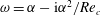
 $\unicode[STIX]{x1D714}=4.862+0.340\text{i}$
corresponds to a wake-dominated mode denoted the principal wake instability. The spectrum is annotated to help provide a physical description of each branch of the spectrum.
$\unicode[STIX]{x1D714}=4.862+0.340\text{i}$
corresponds to a wake-dominated mode denoted the principal wake instability. The spectrum is annotated to help provide a physical description of each branch of the spectrum.
3.3 The discrete branches
The discrete branch of the temporal spectrum shows an exponential instability whose structure is shown in figure 6 and is termed the principal wake instability. Figure 6(a) indicates (by a red circle) the location of the eigenvalue within the bi-global spectrum, (b) shows iso-surfaces of the
 $Q$
-criterion of the perturbation velocity for
$Q$
-criterion of the perturbation velocity for
 $Q=\pm 0.01$
, visualized in blue and red, respectively. The contour slice of the streamwise
$Q=\pm 0.01$
, visualized in blue and red, respectively. The contour slice of the streamwise
 $U$
-velocity of the base flow is projected at
$U$
-velocity of the base flow is projected at
 $x=1$
to provide reference to the location of the wake and vortex region. Figure 6(c) shows the streamwise vorticity of the eigenfunction, with the solid and dashed lines visualizing positive and negative vorticity, respectively.
$x=1$
to provide reference to the location of the wake and vortex region. Figure 6(c) shows the streamwise vorticity of the eigenfunction, with the solid and dashed lines visualizing positive and negative vorticity, respectively.

Figure 6. Bi-global principal wake instability mode. (a) The eigenvalue spectrum plotted with the corresponding eigenvalue circled in red. (b) Shows iso-surfaces of the
 $Q$
-criterion of the perturbation velocity with
$Q$
-criterion of the perturbation velocity with
 $Q=\pm 0.01$
(blue and red, respectively). The contour slice orients the figure to indicate where the wake is located. (c) Shows the streamwise vorticity with solid line contours representing positive vorticity and dashed-lined contours denoting negative vorticity. For a movie of (c), see movie 1 in the supplemental material.
$Q=\pm 0.01$
(blue and red, respectively). The contour slice orients the figure to indicate where the wake is located. (c) Shows the streamwise vorticity with solid line contours representing positive vorticity and dashed-lined contours denoting negative vorticity. For a movie of (c), see movie 1 in the supplemental material.
As the flow leaves the trailing edge, the wake of the wing contains a streamwise velocity deficit. This deficit confines the wake instabilities and reduces the phase speed of the disturbances in this region, with the velocity gradients of the base flow shearing the disturbance, as shown by the aft-angle defined by the red and blue iso-surfaces. Little spanwise variation is present in this mode until the vortex is reached. The rapid decay of the mode as the disturbance approaches the vortex suggests an inhibitive effect of the rotational motion on the wake mode; however, as the instability grows, a helical vortex component that co-rotates with the base flow (see e.g. movie 1 of the supplemental material available at https://doi.org/10.1017/jfm.2017.866) becomes apparent that establishes a coupling between the wake and the vortex. As shown from the figure 6(c), the perturbation is clearly localized to the base-flow shear, decaying exponentially outwards toward the free stream. Similar to many previously studied shear flows, the regions of shear act similar to walls, containing the mode within its critical layers and showing evanescent decay outside.
Progressing farther down the wake branch we encounter a second instability with
 $\unicode[STIX]{x1D714}=4.813+0.1908\text{i}$
, labelled the higher-order wake instability. The corresponding bi-global eigenfunction, shown in figure 7, contains disturbances localized in both regions of the wake and the vortex. The structure of this instability is similar to the principal wake instability (figure 6); however, it contains a spanwise structure with a higher wavenumber in this coordinate direction. The appearance of smaller scales in the spanwise direction gives rise to larger viscous diffusion and, consequently, a lower growth rate relative to the principal wake instability. Similar to the principal wake instability, the disturbance is localized in the region of shear and exponentially decays in the free stream (see figure 7
c). The vortex region just inboard of
$\unicode[STIX]{x1D714}=4.813+0.1908\text{i}$
, labelled the higher-order wake instability. The corresponding bi-global eigenfunction, shown in figure 7, contains disturbances localized in both regions of the wake and the vortex. The structure of this instability is similar to the principal wake instability (figure 6); however, it contains a spanwise structure with a higher wavenumber in this coordinate direction. The appearance of smaller scales in the spanwise direction gives rise to larger viscous diffusion and, consequently, a lower growth rate relative to the principal wake instability. Similar to the principal wake instability, the disturbance is localized in the region of shear and exponentially decays in the free stream (see figure 7
c). The vortex region just inboard of
 $(y,z)=(0,0)$
also shows a helical vortex structure that co-rotates with the base flow (see movie 2 of the supplemental material).
$(y,z)=(0,0)$
also shows a helical vortex structure that co-rotates with the base flow (see movie 2 of the supplemental material).

Figure 7. Bi-global wake instability mode. Variables are plotted following the same format as in figure 6. For a movie of (c), see movie 2 in the supplemental material.
Although the vortex instability, shown in figure 8, has the lowest growth rate (
 $\unicode[STIX]{x1D714}_{i}=0.146$
) of all unstable bi-global modes, its growth rate is comparable to the higher-order wake instability. This type of instability is localized in the vortex core, where the base-flow velocity is larger than in the wake, as reflected in a phase speed higher than for the other instabilities. Due to its localization in the vortex core, we hypothesize that the tip vortex drives this mode.
$\unicode[STIX]{x1D714}_{i}=0.146$
) of all unstable bi-global modes, its growth rate is comparable to the higher-order wake instability. This type of instability is localized in the vortex core, where the base-flow velocity is larger than in the wake, as reflected in a phase speed higher than for the other instabilities. Due to its localization in the vortex core, we hypothesize that the tip vortex drives this mode.
The vortex instability shows a two-lobed structure that co-rotates with the base flow. This pattern may be analogous to the helical mode of vortex instabilities. However, the azimuthal inhomogeneity of the base flow precludes an exact decomposition of the helical nature into Fourier modes (i.e. with azimuthal wavenumbers
 $m$
of integer values). Nonetheless, the observed co-rotation with the base flow hints at an azimuthal mode with
$m$
of integer values). Nonetheless, the observed co-rotation with the base flow hints at an azimuthal mode with
 $m=1$
(see movie 3 of the supplemental material), contrary to the Batchelor vortex which shows an instability for the
$m=1$
(see movie 3 of the supplemental material), contrary to the Batchelor vortex which shows an instability for the
 $m=-1$
mode (Khorrami Reference Khorrami1991; Mayer & Powell Reference Mayer and Powell1992). This implies that the presence of the wake significantly alters the instability properties and furthermore necessitates one to cautiously treat the implication of an analysis of the trailing-line vortex in isolation from the wake. Although the disturbance is localized in the vortex region, the disturbance exists inboard of the vortex region, showing a slight coupling with the wake.
$m=-1$
mode (Khorrami Reference Khorrami1991; Mayer & Powell Reference Mayer and Powell1992). This implies that the presence of the wake significantly alters the instability properties and furthermore necessitates one to cautiously treat the implication of an analysis of the trailing-line vortex in isolation from the wake. Although the disturbance is localized in the vortex region, the disturbance exists inboard of the vortex region, showing a slight coupling with the wake.

Figure 8. Bi-global vortex instability mode. Variables are plotted following the same format as in figure 6. For a movie of (c), see movie 3 in the supplemental material.
Continuing down the vortex branch, a stable vortex mode is shown in figure 9. This mode again shows a two-lobed structure that co-rotates with the base flow, but also contains higher-order structures inboard and beneath the vortex region, reminiscent of the trend along the wake branch. As time increases, the disturbance convects inboard from the tip region with a co-rotating helical mode, as shown in movie 4 of the supplemental material. For eigenfunctions farther down the vortex branch, not shown for brevity, higher-order structures appear in the vortex and a more pronounced interaction with the wake develops, together with increasingly smaller spanwise modal scales.

Figure 9. Bi-global stable vortex mode. Variables are plotted following the same format as in figure 6. For a movie of (c), see movie 4 in the supplemental material.
Farther along the wake branch, shown in figure 10, the slow-phase-speed mode remains restricted to the wake region. A spanwise variation of the mode is clearly visible, showing three lobes across the span. The modal component in the vortex region again represents a two-lobed structure akin to a helical mode that co-rotates with the base flow (see movie 5 of the supplemental material). Progressing farther down the branch (not shown), we encounter an increase in spanwise structures, while the helical nature of the vortex region remains virtually constant.

Figure 10. Bi-global stable wake mode. Variables are plotted following the same format as in figure 6. For a movie of (c), see movie 5 in the supplemental material.
From the analysis of the discrete branches of the bi-global spectrum, some general observations are worth noting. The unstable region of the discrete branch decomposes into two sub-branches which capture (i) a coupled dynamics of the wake–vortex system, and (ii) the instabilities of the vortex core. The principal instability arises on the wake branch for a structure that is predominately wake dominated with a coupled component in the vortex region. The remaining two instabilities, from each of the branches, show similar growth rates, but differ in phase velocity. The vortical components of higher modes show two-lobed structures that co-rotate with the base-flow vorticity – in contrast to the stability behaviour of a Batchelor vortex that counter-rotates with the base flow. This discrepancy points towards a significant effect of the wake component on the dynamics of the trailing vortex in this intermediate region. We hypothesize that the presence of the wake aft of the wing imparts preference to the vortex modes to co-rotate with the base flow, shown in movies 1–5 of the supplemental material. Advancing along both branches towards larger decay rates, an increase in spanwise structures is observed in the wake, as is a more pronounced coupling between the wake and vortex dynamics.
3.4 The continuous branch
While the discrete part of the bi-global spectrum is dictated by the presence of shear in the base-flow velocity field, the fact that we consider viscous flow in an infinite domain introduces a continuous spectrum. This phenomenon has long been recognized and studied in simpler flows such as the Blasius boundary layer (Mack Reference Mack1976; Grosch & Salwen Reference Grosch and Salwen1978). In order to study the continuous branch, we relax the boundary condition at infinity and allow disturbances that are merely bounded at the computational boundary, and thus oscillate in the free stream. Physically, this part of the bi-global spectrum contains information about the interaction characteristics of free-stream perturbations with their discrete counterparts, and thus describes receptivity processes (Saric, Reed & Kerschen Reference Saric, Reed and Kerschen2002). The dispersion relation associated with the continuous spectrum gives insight into the filter behaviour of the flow to external perturbations. This type of analysis uncovers which far-field perturbations interact with the discrete instabilities and which perturbations do not pass the shear region to trigger modal growth.
Following standard procedure (see e.g. Schmid & Henningson Reference Schmid and Henningson2001), we derive an analytical expression for the continuous spectrum by taking the limit as
 $|y|,|z|\rightarrow \infty$
, eliminating base-flow gradients and allowing the approximation of
$|y|,|z|\rightarrow \infty$
, eliminating base-flow gradients and allowing the approximation of
 $(U,V,W)=(U_{\infty },0,0)$
. This step reduces the governing equations to a system of partial differential equations with constant coefficients and thus allows solutions of the form
$(U,V,W)=(U_{\infty },0,0)$
. This step reduces the governing equations to a system of partial differential equations with constant coefficients and thus allows solutions of the form
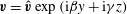 $\boldsymbol{v}=\hat{\boldsymbol{v}}\exp (\text{i}\unicode[STIX]{x1D6FD}y+\text{i}\unicode[STIX]{x1D6FE}z)$
with
$\boldsymbol{v}=\hat{\boldsymbol{v}}\exp (\text{i}\unicode[STIX]{x1D6FD}y+\text{i}\unicode[STIX]{x1D6FE}z)$
with
 $\unicode[STIX]{x1D6FD}$
and
$\unicode[STIX]{x1D6FD}$
and
 $\unicode[STIX]{x1D6FE}$
denoting wavenumbers in the respective coordinate directions. Upon substitution, we obtain a system of algebraic equations for
$\unicode[STIX]{x1D6FE}$
denoting wavenumbers in the respective coordinate directions. Upon substitution, we obtain a system of algebraic equations for
 $\unicode[STIX]{x1D6FD}$
and
$\unicode[STIX]{x1D6FD}$
and
 $\unicode[STIX]{x1D6FE}$
. To further reduce this system of four equations, we eliminate the streamwise disturbance velocity and pressure by utilizing the continuity equation and streamwise momentum equation, while maintaining the disturbance velocities,
$\unicode[STIX]{x1D6FE}$
. To further reduce this system of four equations, we eliminate the streamwise disturbance velocity and pressure by utilizing the continuity equation and streamwise momentum equation, while maintaining the disturbance velocities,
 $v$
and
$v$
and
 $w$
. This results in an eigenvalue problem of the form
$w$
. This results in an eigenvalue problem of the form
 $$\begin{eqnarray}\displaystyle \hat{{\mathcal{A}}}\hat{\boldsymbol{v}}=\unicode[STIX]{x1D714}\hat{{\mathcal{B}}}\hat{\boldsymbol{v}}, & & \displaystyle\end{eqnarray}$$
where
 $\hat{{\mathcal{A}}}$
and
$\hat{{\mathcal{A}}}$
and
 $\hat{{\mathcal{B}}}$
are derived in appendix B, and
$\hat{{\mathcal{B}}}$
are derived in appendix B, and
 $\hat{\boldsymbol{v}}=(\hat{v},{\hat{w}})^{\text{T}}$
. The eigenvalues then are determined as solutions of a quadratic equation according to
$\hat{\boldsymbol{v}}=(\hat{v},{\hat{w}})^{\text{T}}$
. The eigenvalues then are determined as solutions of a quadratic equation according to
 $$\begin{eqnarray}\displaystyle \unicode[STIX]{x1D714}=\frac{-B\pm \sqrt{B^{2}-4AC}}{2A}, & & \displaystyle\end{eqnarray}$$
with
 $$\begin{eqnarray}\displaystyle A=\unicode[STIX]{x1D6FC}^{2}(\unicode[STIX]{x1D709}^{2}-\unicode[STIX]{x1D6FC}^{2}),\quad B=2\text{i}{\hat{c}}_{\ast }A,\quad C={\hat{c}}_{\ast }^{2}\unicode[STIX]{x1D6FC}^{2}(\unicode[STIX]{x1D6FC}^{2}-\unicode[STIX]{x1D709}^{2}), & & \displaystyle\end{eqnarray}$$
where
 $$\begin{eqnarray}\displaystyle {\hat{c}}_{\ast }=\text{i}\unicode[STIX]{x1D6FC}U_{\infty }+\frac{1}{Re_{c}}(\unicode[STIX]{x1D6FC}^{2}+\unicode[STIX]{x1D709}^{2}),\quad \unicode[STIX]{x1D709}^{2}=\unicode[STIX]{x1D6FD}^{2}+\unicode[STIX]{x1D6FE}^{2}. & & \displaystyle\end{eqnarray}$$
Restricting ourselves to real wavenumbers, i.e.
 $\unicode[STIX]{x1D6FD},\unicode[STIX]{x1D6FE}\in \mathbb{R}$
, yields an expression for the classical continuous branch: a line that extends from
$\unicode[STIX]{x1D6FD},\unicode[STIX]{x1D6FE}\in \mathbb{R}$
, yields an expression for the classical continuous branch: a line that extends from
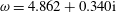
 $\unicode[STIX]{x1D714}=\unicode[STIX]{x1D6FC}-(\unicode[STIX]{x1D6FC}^{2}/Re)\,\text{i}$
to
$\unicode[STIX]{x1D714}=\unicode[STIX]{x1D6FC}-(\unicode[STIX]{x1D6FC}^{2}/Re)\,\text{i}$
to
 $\unicode[STIX]{x1D714}=\unicode[STIX]{x1D6FC}-\infty \,\text{i}$
. This solution of the continuous branch is shown as a red line in figure 11. The fact that the continuous spectrum is a line, despite a dependence on the two parameters
$\unicode[STIX]{x1D714}=\unicode[STIX]{x1D6FC}-\infty \,\text{i}$
. This solution of the continuous branch is shown as a red line in figure 11. The fact that the continuous spectrum is a line, despite a dependence on the two parameters
 $\unicode[STIX]{x1D6FD}$
and
$\unicode[STIX]{x1D6FD}$
and
 $\unicode[STIX]{x1D6FE}$
, comes from the observation that
$\unicode[STIX]{x1D6FE}$
, comes from the observation that
 $\unicode[STIX]{x1D714}$
depends on
$\unicode[STIX]{x1D714}$
depends on
 $\unicode[STIX]{x1D709}=\sqrt{\unicode[STIX]{x1D6FD}^{2}+\unicode[STIX]{x1D6FE}^{2}}$
not on
$\unicode[STIX]{x1D709}=\sqrt{\unicode[STIX]{x1D6FD}^{2}+\unicode[STIX]{x1D6FE}^{2}}$
not on
 $\unicode[STIX]{x1D6FD}$
and
$\unicode[STIX]{x1D6FD}$
and
 $\unicode[STIX]{x1D6FE}$
individually and thus is only parametrized by a single (composite) wavenumber.
$\unicode[STIX]{x1D6FE}$
individually and thus is only parametrized by a single (composite) wavenumber.
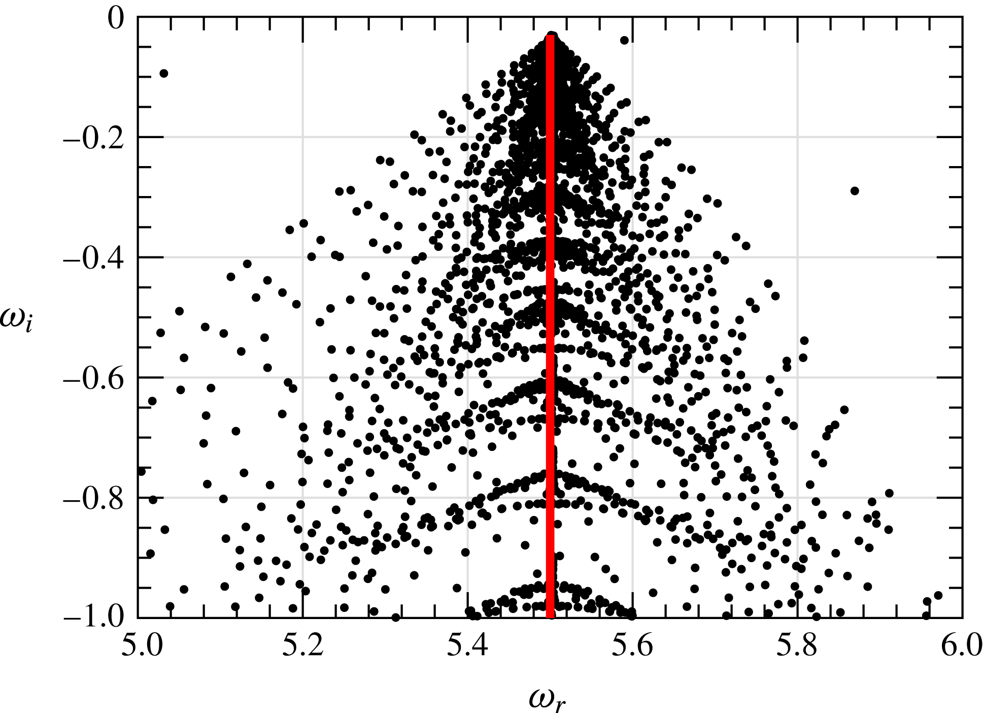
Figure 11. Temporal continuous branch for
 $Re_{c}=1000$
and
$Re_{c}=1000$
and
 $\unicode[STIX]{x1D6FC}=5.5$
for
$\unicode[STIX]{x1D6FC}=5.5$
for
 $N_{y}=N_{z}=80$
. The red line corresponds to the theoretical continuous branch, while the symbols
$N_{y}=N_{z}=80$
. The red line corresponds to the theoretical continuous branch, while the symbols
 $\cdot$
correspond to the numerically computed eigenvalues from the bi-global stability analysis.
$\cdot$
correspond to the numerically computed eigenvalues from the bi-global stability analysis.
The discrete representation of the continuous branch of the bi-global spectrum appears to cover a two-dimensional wedge-like area. Modes that deviate from the analytical continuous branch show exponential decay as they approach the far-field boundary, an observation that has previously been reported (see, e.g. Obrist & Schmid Reference Obrist and Schmid2003a ,Reference Obrist and Schmid b ; Mao & Sherwin Reference Mao and Sherwin2011). Through inspection of the eigenfunctions, we conclude that these modes may be modelled as wavepackets (see § 3.5 for more details).
Eigenfunctions corresponding to eigenvalues along the continuous spectrum have support in the free stream and show oscillations until they reach the computational boundary. Moving down the continuous branch increases the number of oscillations in the free stream, as can also be deduced from the analytical expression (3.2). Modes farther from the continuous branch also oscillate in the free stream, see figure 12 for the eigenvalue
 $\unicode[STIX]{x1D714}=5.154-0.534\text{i}$
, but display an envelope that decays as
$\unicode[STIX]{x1D714}=5.154-0.534\text{i}$
, but display an envelope that decays as
 $(y,z)\rightarrow (\pm \infty ,\infty )$
. As the modes deviate farther from the analytical continuous branch, the decay of the wavepacket envelope becomes increasingly rapid.
$(y,z)\rightarrow (\pm \infty ,\infty )$
. As the modes deviate farther from the analytical continuous branch, the decay of the wavepacket envelope becomes increasingly rapid.

Figure 12. Eigenmode associated with the eigenvalue
 $\unicode[STIX]{x1D714}=5.154-0.534\text{i}$
, which lies off the continuous branch. As in figure 6 with
$\unicode[STIX]{x1D714}=5.154-0.534\text{i}$
, which lies off the continuous branch. As in figure 6 with
 $Q=0.005$
. With the eigenvalue off the continuous branch, the disturbance decays exponentially as it approaches the computational boundary, taking the form of a wavepacket.
$Q=0.005$
. With the eigenvalue off the continuous branch, the disturbance decays exponentially as it approaches the computational boundary, taking the form of a wavepacket.
To further explore this phenomenon, we relax the boundedness condition, used in the derivation of the continuous spectrum, to allow for exponential decay in the free stream. This is equivalent to permitting complex transverse wavenumbers (i.e.
 $\unicode[STIX]{x1D6FD},\unicode[STIX]{x1D6FE}\in \mathbb{C}$
), where the real component corresponds, as before, to the free-stream oscillations, while the imaginary part describes the growth or decay in the transverse directions. This formulation allows for a rudimentary model of wavepackets. Since the disturbances must be bounded, we take the sign of the imaginary part appropriately to enforce exponential decay as we approach the free stream,
$\unicode[STIX]{x1D6FD},\unicode[STIX]{x1D6FE}\in \mathbb{C}$
), where the real component corresponds, as before, to the free-stream oscillations, while the imaginary part describes the growth or decay in the transverse directions. This formulation allows for a rudimentary model of wavepackets. Since the disturbances must be bounded, we take the sign of the imaginary part appropriately to enforce exponential decay as we approach the free stream,
 $(y,z)\rightarrow (\pm \infty ,\infty )$
.
$(y,z)\rightarrow (\pm \infty ,\infty )$
.
With the wavenumbers
 $\unicode[STIX]{x1D6FD}$
and
$\unicode[STIX]{x1D6FD}$
and
 $\unicode[STIX]{x1D6FE}$
allowed to take on complex values, we can map the lower half of the complex
$\unicode[STIX]{x1D6FE}$
allowed to take on complex values, we can map the lower half of the complex
 $(\unicode[STIX]{x1D6FD},\unicode[STIX]{x1D6FE})$
-plane under the analytical expression (3.2) for the continuous spectrum. Figure 13(b) shows the resulting parabolic spread in the complex
$(\unicode[STIX]{x1D6FD},\unicode[STIX]{x1D6FE})$
-plane under the analytical expression (3.2) for the continuous spectrum. Figure 13(b) shows the resulting parabolic spread in the complex
 $c$
-plane. With increasing magnitudes of
$c$
-plane. With increasing magnitudes of
 $\unicode[STIX]{x1D6FD}_{i}$
and
$\unicode[STIX]{x1D6FD}_{i}$
and
 $\unicode[STIX]{x1D6FE}_{i}$
these parabolas spread upward and outward, and the mapped half-plane covers an increasingly larger area of the complex
$\unicode[STIX]{x1D6FE}_{i}$
these parabolas spread upward and outward, and the mapped half-plane covers an increasingly larger area of the complex
 $c$
-plane. It is important to note that these parabolas cover a continuous area; the exact locations of the global eigenvalues in this region, however, are affected by the numerical discretization and the choice of computational domain size and depend sensitively on these numerical parameters.
$c$
-plane. It is important to note that these parabolas cover a continuous area; the exact locations of the global eigenvalues in this region, however, are affected by the numerical discretization and the choice of computational domain size and depend sensitively on these numerical parameters.

Figure 13. The complex
 $(\unicode[STIX]{x1D6FD},\unicode[STIX]{x1D6FE})$
-plane shown in (a) is then mapped to the complex phase-speed plane, where
$(\unicode[STIX]{x1D6FD},\unicode[STIX]{x1D6FE})$
-plane shown in (a) is then mapped to the complex phase-speed plane, where
 $c=\unicode[STIX]{x1D714}/\unicode[STIX]{x1D6FC}$
shown in (b). The complex
$c=\unicode[STIX]{x1D714}/\unicode[STIX]{x1D6FC}$
shown in (b). The complex
 $(\unicode[STIX]{x1D6FD},\unicode[STIX]{x1D6FE})$
results in a continuous spectrum of an area in the complex
$(\unicode[STIX]{x1D6FD},\unicode[STIX]{x1D6FE})$
results in a continuous spectrum of an area in the complex
 $c$
-plane, rather than a line (
$c$
-plane, rather than a line (
 $\unicode[STIX]{x1D6FD}_{i},\unicode[STIX]{x1D6FE}_{i}=0$
) as in classical stability theory.
$\unicode[STIX]{x1D6FD}_{i},\unicode[STIX]{x1D6FE}_{i}=0$
) as in classical stability theory.
3.5 Wavepacket analysis
We proceed by introducing a third manner of analysis of the spectral problem of trailing-line vortices. Our first analysis in § 3.3 solved the full global eigenvalue problem and was particularly suited to regions where the coefficients of our system (given by the base flow and its derivatives) are rapidly varying; this analysis resulted in the discrete modal structures. The second approach in § 3.4 considered the limit of large distances from the regions of shear, where the base flow appears uniform and our system can be approximated by a constant-coefficient set of equations; the resulting wave solutions and the corresponding analytic dispersion relation (3.2) constitute the continuous branch of the spectrum and describe oscillatory modal solutions that spatially continue to infinity. In this section, we address the intermediate regime where eigensolutions can be approximated by compact wavepackets. This approximation becomes exponentially accurate as a small, user-defined parameter, in our case
 $h=1/\sqrt{Re_{c}}$
, tends to zero. This type of analysis covers structures in the outer neighbourhoods of the vortex and wake and sheds light on the remaining global eigenvalues which can neither be identified as discrete nor as continuous. An analysis of this type has been successfully performed in simpler configurations (Obrist & Schmid Reference Obrist and Schmid2010; Mao & Sherwin Reference Mao and Sherwin2011); here, we extend it to a two-dimensional base flow. For the sake of focus, the mathematical details of the methodology are relegated to the appendix C, while the motivation, a conceptual summary, the results and physical interpretation are provided in this section.
$h=1/\sqrt{Re_{c}}$
, tends to zero. This type of analysis covers structures in the outer neighbourhoods of the vortex and wake and sheds light on the remaining global eigenvalues which can neither be identified as discrete nor as continuous. An analysis of this type has been successfully performed in simpler configurations (Obrist & Schmid Reference Obrist and Schmid2010; Mao & Sherwin Reference Mao and Sherwin2011); here, we extend it to a two-dimensional base flow. For the sake of focus, the mathematical details of the methodology are relegated to the appendix C, while the motivation, a conceptual summary, the results and physical interpretation are provided in this section.
Wavepacket analysis helps depict the two-dimensionality of the eigenvalue spectrum of the bi-global analysis through the solution of a system of algebraic equations. This methodology may yield efficient means of computing the spectrum that can be applied to application of transient growth and potential applications such as aeroacoustics where wavepackets are of prime importance. This motivates the extension of wavepacket analysis from the simplified one-dimensional cases shown in Trefethen (Reference Trefethen2005), Obrist & Schmid (Reference Obrist and Schmid2010), Mao & Sherwin (Reference Mao and Sherwin2011) to the two-dimensional case where more complex flows are applicable.
Conceptually, wavepacket analysis assumes eigenfunctions of the general form
 $\exp (\text{i}f(y,z;h))$
with
$\exp (\text{i}f(y,z;h))$
with
 $f$
denoting an unknown phase function that depends on both spatial coordinates as well as a small parameter
$f$
denoting an unknown phase function that depends on both spatial coordinates as well as a small parameter
 $h$
. This approach is reminiscent and akin to a Wentzel–Kramers–Brillouin–Jeffreys (WKBJ) procedure and utilizing wavepacket analysis provides an approximate dispersion relation. Upon substitution of our general form into the governing equations and introducing the spatially local wavenumbers
$h$
. This approach is reminiscent and akin to a Wentzel–Kramers–Brillouin–Jeffreys (WKBJ) procedure and utilizing wavepacket analysis provides an approximate dispersion relation. Upon substitution of our general form into the governing equations and introducing the spatially local wavenumbers
 $\unicode[STIX]{x1D735}f=(f_{y},f_{z})^{\text{T}}\equiv (1/h)(\unicode[STIX]{x1D6FD},\unicode[STIX]{x1D6FE})^{\text{T}}$
, we arrive at a dispersion relation for
$\unicode[STIX]{x1D735}f=(f_{y},f_{z})^{\text{T}}\equiv (1/h)(\unicode[STIX]{x1D6FD},\unicode[STIX]{x1D6FE})^{\text{T}}$
, we arrive at a dispersion relation for
 $\unicode[STIX]{x1D714}$
that depends on both
$\unicode[STIX]{x1D714}$
that depends on both
 $(y,z)$
and the associated wavenumbers
$(y,z)$
and the associated wavenumbers
 $(\unicode[STIX]{x1D6FD},\unicode[STIX]{x1D6FE})$
and thus contains a hybrid of physical and spectral components. This dispersion relation is approximate but approaches the true dispersion relation exponentially as
$(\unicode[STIX]{x1D6FD},\unicode[STIX]{x1D6FE})$
and thus contains a hybrid of physical and spectral components. This dispersion relation is approximate but approaches the true dispersion relation exponentially as
 $h\rightarrow 0$
. Mathematically, this approximate dispersion relation is referred to as the symbol (Trefethen Reference Trefethen2005). Thus far, solutions of the form
$h\rightarrow 0$
. Mathematically, this approximate dispersion relation is referred to as the symbol (Trefethen Reference Trefethen2005). Thus far, solutions of the form
 $\exp (\text{i}f(y,z;h))$
do not necessarily represent wavepackets. Additional constraints have to be imposed to ensure compactness of the eigenfunctions. A simple second-order Taylor expansion about the peak of the wavepacket
$\exp (\text{i}f(y,z;h))$
do not necessarily represent wavepackets. Additional constraints have to be imposed to ensure compactness of the eigenfunctions. A simple second-order Taylor expansion about the peak of the wavepacket
 $\boldsymbol{x}_{\ast }=(y_{\ast },z_{\ast })$
yields (we will use the subscript
$\boldsymbol{x}_{\ast }=(y_{\ast },z_{\ast })$
yields (we will use the subscript
 $_{\ast }$
to denote evaluation at peak location)
$_{\ast }$
to denote evaluation at peak location)
 $$\begin{eqnarray}\displaystyle \exp (\text{i}f(y,z;h))\sim \underbrace{\exp (\text{i}f_{\ast })}_{const.}\times \underbrace{\exp (\text{i}\boldsymbol{b}_{\ast }^{\text{T}}(\boldsymbol{x}-\boldsymbol{x}_{\ast }))}_{carrier~wave}\times \underbrace{\exp (\text{i}(\boldsymbol{x}-\boldsymbol{x}_{\ast })^{\text{T}}\mathsf{C}_{\ast }(\boldsymbol{x}-\boldsymbol{x}_{\ast }))}_{packet~envelope}, & & \displaystyle\end{eqnarray}$$
with
 $\boldsymbol{b}=\unicode[STIX]{x1D735}f$
and
$\boldsymbol{b}=\unicode[STIX]{x1D735}f$
and
 $\mathsf{C}=\unicode[STIX]{x1D6FB}^{2}f$
as the gradient and Hessian of
$\mathsf{C}=\unicode[STIX]{x1D6FB}^{2}f$
as the gradient and Hessian of
 $f$
, respectively. Clearly, a condition on
$f$
, respectively. Clearly, a condition on
 $\mathsf{C}$
has to be imposed to ensure that the wavepacket envelope is compact, rather than divergent. This condition is referred to as the twist condition (Trefethen Reference Trefethen2005) and is given in appendix C.
$\mathsf{C}$
has to be imposed to ensure that the wavepacket envelope is compact, rather than divergent. This condition is referred to as the twist condition (Trefethen Reference Trefethen2005) and is given in appendix C.
The procedural steps of a wavepacket analysis are then as follows. We sweep over
 $y_{\ast }$
and
$y_{\ast }$
and
 $z_{\ast }$
(the peak location of our wavepacket mode), covering the physical domain of interest, e.g. the neighbourhood of the vortex or the wake; simultaneously, we also sweep over the wavenumbers
$z_{\ast }$
(the peak location of our wavepacket mode), covering the physical domain of interest, e.g. the neighbourhood of the vortex or the wake; simultaneously, we also sweep over the wavenumbers
 $\unicode[STIX]{x1D6FD}_{\ast }$
and
$\unicode[STIX]{x1D6FD}_{\ast }$
and
 $\unicode[STIX]{x1D6FE}_{\ast }$
, covering the spatial scales of interest. For each point
$\unicode[STIX]{x1D6FE}_{\ast }$
, covering the spatial scales of interest. For each point
 $(y_{\ast },z_{\ast },\unicode[STIX]{x1D6FD}_{\ast },\unicode[STIX]{x1D6FE}_{\ast })$
we verify the twist condition and discard points that do not satisfy it, deeming them unphysical. The accepted points are then mapped, via the symbol (i.e. approximate dispersion relation), into the complex domain where they trace out a parameterized curve as
$(y_{\ast },z_{\ast },\unicode[STIX]{x1D6FD}_{\ast },\unicode[STIX]{x1D6FE}_{\ast })$
we verify the twist condition and discard points that do not satisfy it, deeming them unphysical. The accepted points are then mapped, via the symbol (i.e. approximate dispersion relation), into the complex domain where they trace out a parameterized curve as
 $(y_{\ast },z_{\ast },\unicode[STIX]{x1D6FD}_{\ast },\unicode[STIX]{x1D6FE}_{\ast })$
are varied. Each point on this curve constitutes an (exponentially) approximate eigenvalue associated with our wavepacket eigenmode. Depending on the complexity of the symbol, these curves can intersect one another on the complex plane, giving rise to multiple wavepacket solutions. The parameterization by four parameters
$(y_{\ast },z_{\ast },\unicode[STIX]{x1D6FD}_{\ast },\unicode[STIX]{x1D6FE}_{\ast })$
are varied. Each point on this curve constitutes an (exponentially) approximate eigenvalue associated with our wavepacket eigenmode. Depending on the complexity of the symbol, these curves can intersect one another on the complex plane, giving rise to multiple wavepacket solutions. The parameterization by four parameters
 $(y_{\ast },z_{\ast },\unicode[STIX]{x1D6FD}_{\ast },\unicode[STIX]{x1D6FE}_{\ast })$
generally yields an area in the complex plane that constitutes the spectral location of approximate wavepacket solutions to our stability problem. The wedge-like clustering of discrete points about the continuous spectrum in figure 5 about
$(y_{\ast },z_{\ast },\unicode[STIX]{x1D6FD}_{\ast },\unicode[STIX]{x1D6FE}_{\ast })$
generally yields an area in the complex plane that constitutes the spectral location of approximate wavepacket solutions to our stability problem. The wedge-like clustering of discrete points about the continuous spectrum in figure 5 about
 $\unicode[STIX]{x1D714}_{r}\approx 5.5$
is a (discrete) manifestation of this area spectrum. For more details, refer to appendix C.
$\unicode[STIX]{x1D714}_{r}\approx 5.5$
is a (discrete) manifestation of this area spectrum. For more details, refer to appendix C.
The symbol can be used to assess the characteristics of the bi-global eigenvalue spectrum. In figure 14(a), we select an eigenvalue (circled in red) to compare the true eigenmode from our bi-global analysis with the corresponding approximate mode computed through wavepacket analysis. To this end, we determine the parameters
 $y_{\ast }$
and
$y_{\ast }$
and
 $z_{\ast }$
, i.e. the location of the wavepacket, using (C 5) and
$z_{\ast }$
, i.e. the location of the wavepacket, using (C 5) and
 $\unicode[STIX]{x1D6FD}_{\ast }/h$
,
$\unicode[STIX]{x1D6FD}_{\ast }/h$
,
 $\unicode[STIX]{x1D6FE}_{\ast }/h,$
i.e. the approximate wavenumbers, using (C 4). We then substitute these parameters into (C 5) to obtain four distinct wavepackets. Although this provides the location and shape of the wavepackets, the weighting of each individual approximation is still unknown. We use the eigenfunction from the bi-global spectrum and minimize the least-squares error between a linear combination of approximations and the true eigenfunction. The resulting streamwise vorticity is shown in figure 14(b). Comparing the superposition of the wavepacket modes with the bi-global eigenfunction in figure 14(c), we see that the wavepackets capture the location and direction of the global mode, but lack the curvature of the wavefronts in the global structure near
$\unicode[STIX]{x1D6FE}_{\ast }/h,$
i.e. the approximate wavenumbers, using (C 4). We then substitute these parameters into (C 5) to obtain four distinct wavepackets. Although this provides the location and shape of the wavepackets, the weighting of each individual approximation is still unknown. We use the eigenfunction from the bi-global spectrum and minimize the least-squares error between a linear combination of approximations and the true eigenfunction. The resulting streamwise vorticity is shown in figure 14(b). Comparing the superposition of the wavepacket modes with the bi-global eigenfunction in figure 14(c), we see that the wavepackets capture the location and direction of the global mode, but lack the curvature of the wavefronts in the global structure near
 $y<0$
,
$y<0$
,
 $z\approx 0$
. A slice across the vortex core along
$z\approx 0$
. A slice across the vortex core along
 $z=0$
is shown in figure 14(d), with the blue line representing the wavepacket results and the black line designating the global results. The red lines indicate where the individual wavepackets are centred (i.e. the value of
$z=0$
is shown in figure 14(d), with the blue line representing the wavepacket results and the black line designating the global results. The red lines indicate where the individual wavepackets are centred (i.e. the value of
 $y_{\ast }$
). A reasonable match between the bi-global analysis and the wavepacket analysis is observed.
$y_{\ast }$
). A reasonable match between the bi-global analysis and the wavepacket analysis is observed.

Figure 14. Comparison of wavepackets to bi-global spectrum for the four wavepackets nearest to the eigenvalue
 $\unicode[STIX]{x1D714}=5.220-\text{i}0.501$
. (a) Shows the eigenvalue spectrum with the eigenvalue examined circled in red. (b) Shows the weighted sum over the four wavepackets from the wavepacket analysis. (c) Shows the bi-global eigenmode corresponding to the circled eigenvalue. (d) Is the projection of the disturbance velocity,
$\unicode[STIX]{x1D714}=5.220-\text{i}0.501$
. (a) Shows the eigenvalue spectrum with the eigenvalue examined circled in red. (b) Shows the weighted sum over the four wavepackets from the wavepacket analysis. (c) Shows the bi-global eigenmode corresponding to the circled eigenvalue. (d) Is the projection of the disturbance velocity,
 $v$
, along the line
$v$
, along the line
 $z=0$
, showing how the wavepackets (blue) compares with the bi-global spectrum (black). The red lines denote the wavepacket locations.
$z=0$
, showing how the wavepackets (blue) compares with the bi-global spectrum (black). The red lines denote the wavepacket locations.
Due to the nature of wavepacket solutions and our access to an (approximate) analytical expression for the dispersion relation, we are in a position to explore and quantify the travel direction of modal wavepacket structure. We simply examine the group velocity,
 $\unicode[STIX]{x2202}\unicode[STIX]{x1D714}/\unicode[STIX]{x2202}\boldsymbol{k}$
, where
$\unicode[STIX]{x2202}\unicode[STIX]{x1D714}/\unicode[STIX]{x2202}\boldsymbol{k}$
, where
 $\boldsymbol{k}$
denotes the wavenumber vector with
$\boldsymbol{k}$
denotes the wavenumber vector with
 $\unicode[STIX]{x1D6FD}_{\ast }$
and
$\unicode[STIX]{x1D6FD}_{\ast }$
and
 $\unicode[STIX]{x1D6FE}_{\ast }$
aligning with the
$\unicode[STIX]{x1D6FE}_{\ast }$
aligning with the
 $y$
- and
$y$
- and
 $z$
-directions, respectively. More specifically, an approximation of the group velocity can be extracted directly from the terms in the twist condition,
$z$
-directions, respectively. More specifically, an approximation of the group velocity can be extracted directly from the terms in the twist condition,
 $\unicode[STIX]{x2202}f/\unicode[STIX]{x2202}\unicode[STIX]{x1D6FD}_{\ast }$
and
$\unicode[STIX]{x2202}f/\unicode[STIX]{x2202}\unicode[STIX]{x1D6FD}_{\ast }$
and
 $\unicode[STIX]{x2202}f/\unicode[STIX]{x2202}\unicode[STIX]{x1D6FE}_{\ast }$
in (C 4). The group velocity of the dominant wavepacket (with the largest coefficient in the above superposition) shows that the disturbance travels inbound towards the vortex core, as indicated by arrows in figure 15(a,b). This inboard direction is congruent with the results from the bi-global analysis (see e.g. movie 4 of the supplemental material). Interestingly, although the velocity field appears outside the region of shear, the associated pressure field remains confined within the shear region as shown in figure 15(b). This may suggest a particular receptive behaviour whereby velocity disturbances in the far field trigger disturbances in the shear region via pressure perturbations, followed by a transfer of energy to the unstable discrete branch or transient growth. The interaction of free-stream disturbances with regions of shear is a common feature in receptivity studies (Saric et al.
Reference Saric, Reed and Kerschen2002). The underlying mechanism behind this transfer from vorticity to pressure requires further research but may be a result of non-normality of the eigenvectors.
$\unicode[STIX]{x2202}f/\unicode[STIX]{x2202}\unicode[STIX]{x1D6FE}_{\ast }$
in (C 4). The group velocity of the dominant wavepacket (with the largest coefficient in the above superposition) shows that the disturbance travels inbound towards the vortex core, as indicated by arrows in figure 15(a,b). This inboard direction is congruent with the results from the bi-global analysis (see e.g. movie 4 of the supplemental material). Interestingly, although the velocity field appears outside the region of shear, the associated pressure field remains confined within the shear region as shown in figure 15(b). This may suggest a particular receptive behaviour whereby velocity disturbances in the far field trigger disturbances in the shear region via pressure perturbations, followed by a transfer of energy to the unstable discrete branch or transient growth. The interaction of free-stream disturbances with regions of shear is a common feature in receptivity studies (Saric et al.
Reference Saric, Reed and Kerschen2002). The underlying mechanism behind this transfer from vorticity to pressure requires further research but may be a result of non-normality of the eigenvectors.

Figure 15. (a) The streamwise vorticity for the eigenvalue
 $\unicode[STIX]{x1D714}=5.220-\text{i}0.501$
and (b) the corresponding disturbance pressure. The solid contour lines denoting the location of the wake and the base of the arrow is the location of the wavepacket. The direction of the arrow indicates the group velocity,
$\unicode[STIX]{x1D714}=5.220-\text{i}0.501$
and (b) the corresponding disturbance pressure. The solid contour lines denoting the location of the wake and the base of the arrow is the location of the wavepacket. The direction of the arrow indicates the group velocity,
 $\unicode[STIX]{x2202}\unicode[STIX]{x1D714}/\unicode[STIX]{x2202}\boldsymbol{k}$
, of the wavepacket.
$\unicode[STIX]{x2202}\unicode[STIX]{x1D714}/\unicode[STIX]{x2202}\boldsymbol{k}$
, of the wavepacket.
Although figures 14 and 15 provide a single wavepacket, how the wavepackets vary across the continuous branch wedge is now examined qualitatively for the sake of brevity. When approaching the region near the analytical continuous branch in figure 13, the envelope of the wavepacket analysis broadens in the free stream, approaching the free-stream oscillation limit. Conversely, as the discrete branch is approached, the energy of the wavepacket is more compact and approaches the regions of shear. This physically aligns with continuous branch and discrete branch limits of the wavepacket analysis, matching well with the bi-global analysis and further providing confidence in the method.
This concludes the temporal stability analysis, which examined and identifies three distinct types of instabilities from the discrete spectrum, and assessed the continuous spectrum far from the shear flow. We then explored approximate wavepacket solutions. We now proceed to complement the temporal results with a spatial stability analysis.
4 Spatial bi-global stability analysis
We begin the spatial analysis by first parametrically sweeping through the frequency and, drawing upon similarities with the temporal spectrum, choose to analyse a frequency of
 $\unicode[STIX]{x1D714}=5.5$
. Then, we present the spatial eigenvalue spectrum and compare it with the temporal spectrum, highlighting similarities through the complex phase speed, followed by discussions on various spatial instabilities. We conclude with explaining some peculiarities associated with the spatial continuous branch.
$\unicode[STIX]{x1D714}=5.5$
. Then, we present the spatial eigenvalue spectrum and compare it with the temporal spectrum, highlighting similarities through the complex phase speed, followed by discussions on various spatial instabilities. We conclude with explaining some peculiarities associated with the spatial continuous branch.
4.1 Frequency parameterization
By sweeping the frequency from
 $\unicode[STIX]{x1D714}=2$
to 8 in increments of
$\unicode[STIX]{x1D714}=2$
to 8 in increments of
 $\unicode[STIX]{x0394}\unicode[STIX]{x1D714}=0.5$
, we observe a number of instabilities including the addition of a vortex instability that contains high growth at low frequencies as shown in figure 16. Aside from this instability, the frequency sweep in figure 16 follows similar trends to the wavenumber sweep of the temporal analysis, shown in figure 4, containing principal wake, wake and vortex instabilities. As the spatial and temporal parametric sweeps contain similar structures, we choose to examine the frequency counterpart to the temporal analysis, which corresponds to
$\unicode[STIX]{x0394}\unicode[STIX]{x1D714}=0.5$
, we observe a number of instabilities including the addition of a vortex instability that contains high growth at low frequencies as shown in figure 16. Aside from this instability, the frequency sweep in figure 16 follows similar trends to the wavenumber sweep of the temporal analysis, shown in figure 4, containing principal wake, wake and vortex instabilities. As the spatial and temporal parametric sweeps contain similar structures, we choose to examine the frequency counterpart to the temporal analysis, which corresponds to
 $\unicode[STIX]{x1D714}=5.5$
indicated by the dashed line in figure 16.
$\unicode[STIX]{x1D714}=5.5$
indicated by the dashed line in figure 16.

Figure 16. Spatial growth rate,
 $-\unicode[STIX]{x1D6FC}_{i}$
, at
$-\unicode[STIX]{x1D6FC}_{i}$
, at
 $x=3$
with varying frequency
$x=3$
with varying frequency
 $\unicode[STIX]{x1D714}$
, with
$\unicode[STIX]{x1D714}$
, with
 $N_{z}=N_{y}=60$
. The four instabilities are labelled as wake mode, primary vortex mode, wake mode and secondary vortex mode according to their modal features. The dashed line indicates the wavenumber that we examined throughout the temporal analysis.
$N_{z}=N_{y}=60$
. The four instabilities are labelled as wake mode, primary vortex mode, wake mode and secondary vortex mode according to their modal features. The dashed line indicates the wavenumber that we examined throughout the temporal analysis.
4.2 Eigenvalue spectrum and its comparison with the temporal spectrum
Due to the ansatz in (2.2), the eigenvalue spectrum for the spatial analysis inverts such that modally unstable eigenvalues reside in the lower half-plane
 $\unicode[STIX]{x1D6FC}_{i}<0$
, as shown by the grey region in figure 17(a). The discrete spectrum now sweeps over an area upward from
$\unicode[STIX]{x1D6FC}_{i}<0$
, as shown by the grey region in figure 17(a). The discrete spectrum now sweeps over an area upward from
 $\unicode[STIX]{x1D6FC}\approx \unicode[STIX]{x1D714}+\text{i}\unicode[STIX]{x1D714}^{2}/Re$
, with discrete branches to its right and a single discrete branch to its left. The discrete branches right of the continuous spectrum contain a vortex and wake branch, analogous to their temporal counterparts. An additional third branch contains vortex modes to the farther right than the wake branch. The branch left of the continuous spectrum is analogous to the discrete branch to the right of the temporal continuous branch, which corresponds to higher-order azimuthal modes.
$\unicode[STIX]{x1D6FC}\approx \unicode[STIX]{x1D714}+\text{i}\unicode[STIX]{x1D714}^{2}/Re$
, with discrete branches to its right and a single discrete branch to its left. The discrete branches right of the continuous spectrum contain a vortex and wake branch, analogous to their temporal counterparts. An additional third branch contains vortex modes to the farther right than the wake branch. The branch left of the continuous spectrum is analogous to the discrete branch to the right of the temporal continuous branch, which corresponds to higher-order azimuthal modes.

Figure 17. The spatial eigenvalue spectrum for
 $\unicode[STIX]{x1D714}=5.5$
in the complex
$\unicode[STIX]{x1D714}=5.5$
in the complex
 $\unicode[STIX]{x1D6FC}$
-plane, (a), and in the complex phase-speed plane, (b). In (b), the equivalent temporal spectrum is shown for
$\unicode[STIX]{x1D6FC}$
-plane, (a), and in the complex phase-speed plane, (b). In (b), the equivalent temporal spectrum is shown for
 $\unicode[STIX]{x1D6FC}=5.5$
, denoted by the red circles. For comparison, the pertinent discrete branches are labelled.
$\unicode[STIX]{x1D6FC}=5.5$
, denoted by the red circles. For comparison, the pertinent discrete branches are labelled.
The temporal and spatial spectra possess many similar features. For a more direct comparison, figure 17(b) compares the temporal spectrum (red circles) to the spatial spectrum (black dots) in the complex phase-speed plane,
 $c=\unicode[STIX]{x1D714}/\unicode[STIX]{x1D6FC}$
. In the
$c=\unicode[STIX]{x1D714}/\unicode[STIX]{x1D6FC}$
. In the
 $c$
-plane, the two spectra align, with the wake and vortex branches in the temporal analysis aligning with the corresponding branches in the spatial spectrum. The leftmost vortex branch in figure 17(b) aligns with stable modes in the temporal spectrum. The continuous branches sweep over approximately the same area, except that the spatial spectrum bends left as
$c$
-plane, the two spectra align, with the wake and vortex branches in the temporal analysis aligning with the corresponding branches in the spatial spectrum. The leftmost vortex branch in figure 17(b) aligns with stable modes in the temporal spectrum. The continuous branches sweep over approximately the same area, except that the spatial spectrum bends left as
 $c_{r}$
decreases – a phenomenon that is explained in § 4.4.
$c_{r}$
decreases – a phenomenon that is explained in § 4.4.
The alignment of the temporal and spatial eigenvalue spectra in
 $c$
-space has relevance to Gaster’s transformation (Gaster Reference Gaster1962), which holds for regions near the neutral stability curve. Gaster (Reference Gaster1962) showed that for small growth rates, the temporal and spatial growth rates can be related through the group velocity,
$c$
-space has relevance to Gaster’s transformation (Gaster Reference Gaster1962), which holds for regions near the neutral stability curve. Gaster (Reference Gaster1962) showed that for small growth rates, the temporal and spatial growth rates can be related through the group velocity,
 $c_{g}=\unicode[STIX]{x2202}\unicode[STIX]{x1D714}_{r}/\unicode[STIX]{x2202}\unicode[STIX]{x1D6FC}_{r}$
. From the relatively good alignment of the temporal and spatial spectra in
$c_{g}=\unicode[STIX]{x2202}\unicode[STIX]{x1D714}_{r}/\unicode[STIX]{x2202}\unicode[STIX]{x1D6FC}_{r}$
. From the relatively good alignment of the temporal and spatial spectra in
 $c$
-space, we conclude that the deviation of the spectra is a result of the fairly large growth rates. Furthermore, the group velocity of the modes can be approximated, showing that these instabilities (and modes in general) are convective in nature.
$c$
-space, we conclude that the deviation of the spectra is a result of the fairly large growth rates. Furthermore, the group velocity of the modes can be approximated, showing that these instabilities (and modes in general) are convective in nature.
4.3 Discrete spatial bi-global modes
The striking similarities between the temporal and spatial spectra suggest that the two spectra contain analogous eigenmodes on the matching branches. Thus, we expect the most unstable eigenvalue to represent a wake mode, similar to its temporal counterpart, which is confirmed in figure 18 (and movie 6 of the supplemental material). Comparing figure 18 with its temporal counterpart (figure 6), we observe that the disturbances remain localized to the wake region and contain nearly identical structures, which instead grow with downstream progression because of their instability. Furthermore, this instability has no spanwise zero crossings until the vortex is reached, again highlighting that the wake aft of the wing is the cause of this instability.

Figure 18. Bi-global spatial principal wake instability mode. Variables are plotted following the same format as in figure 6 with
 $Q=\pm 0.0001$
. For a movie of (c), see movie 6 in the supplemental material.
$Q=\pm 0.0001$
. For a movie of (c), see movie 6 in the supplemental material.
From these similarities, we expect that the modes farther down the wake branch contain higher-order spanwise structures, seen in the third instability shown in figure 19 (supplementary movie 7). This mode, lying close to its analogous temporal mode (see figure 7), contains a higher number of zero crossings, indicating a higher spanwise wavenumber. The same mode, however, decays more rapidly in the vicinity of the vortex. If we continue down this branch, we follow the same trend shown in the temporal section of higher-order spanwise structures in the wake region. Moreover, we argue that the reduced structure size and increased viscous effects cause the stabilization of these modes.

Figure 19. Bi-global spatial wake instability mode. Variables are plotted following the same format as in figure 6 with
 $Q=\pm 0.0001$
. For a movie of (c), see movie 7 in the supplemental material.
$Q=\pm 0.0001$
. For a movie of (c), see movie 7 in the supplemental material.
Continuing with the temporal analogues, along the vortex branch we observe that the disturbances are localized to the vortex region, with a wavepacket below it; compare figure 20 (supplementary movie 8) with figure 8. Contrary to the temporal mode, the vortex mode from the spatial analysis contains a complex vortex structure rather than the two-lobed structure that co-rotates with the base flow as in its temporal counterpart. The complex structure and wake aligns better with higher-order temporal vortex modes as shown in figure 9. Continuing down this branch confirms that the wavepacket contains higher-order modes.

Figure 20. Bi-global secondary spatial vortex instability mode. Variables are plotted following the same format as in figure 6 with
 $Q=\pm 0.0001$
. For a movie of (c), see movie 8 in the supplemental material.
$Q=\pm 0.0001$
. For a movie of (c), see movie 8 in the supplemental material.
From the spatial analysis, a new instability emerged, which is linked solely to the vortex region, with only fringe amounts of the disturbance localized in the wake, shown in figure 21 (supplementary movie 9). This instability contains a two-lobed structure where the inboard lobe originates from the region where the vortex and wake pinch off to separate, and the other lobe coming from the vortex core region. The rotation of this mode is difficult to discern with the disturbances traveling in the upward and inboard direction. Higher-order modes further down this branch contain smaller-scale structures in the transverse direction and comprise more disturbances in the wake region.

Figure 21. Bi-global primary spatial vortex instability mode. Variables are plotted following the same format as in figure 6 with
 $Q=\pm 0.0001$
. For a movie of (c), see movie 9 in the supplemental material.
$Q=\pm 0.0001$
. For a movie of (c), see movie 9 in the supplemental material.
The final mode we examine lies on a discrete branch to the right of the continuous spectrum in the
 $c$
-plane. This branch, termed the azimuthal branch in § 3.2, contains vortex modes with higher azimuthal wavenumbers. The mode chosen in figure 22 is an
$c$
-plane. This branch, termed the azimuthal branch in § 3.2, contains vortex modes with higher azimuthal wavenumbers. The mode chosen in figure 22 is an
 $(m=3)$
-mode that co-rotates with the flow (see supplementary movie 10) and is confined to the vortex region of the base flow. Modes on this branch may be significant at different frequencies, as Paredes (Reference Paredes2014) shows that higher-order modes contain higher growth rates in the spatial analysis of the Batchelor vortex; however, higher frequencies are beyond the scope of this study.
$(m=3)$
-mode that co-rotates with the flow (see supplementary movie 10) and is confined to the vortex region of the base flow. Modes on this branch may be significant at different frequencies, as Paredes (Reference Paredes2014) shows that higher-order modes contain higher growth rates in the spatial analysis of the Batchelor vortex; however, higher frequencies are beyond the scope of this study.

Figure 22. Bi-global spatial higher-order azimuthal mode. Variables are plotted following the same format as in figure 6 with
 $Q=\pm 0.0001$
. For a movie of (c), see movie 10 in the supplemental material.
$Q=\pm 0.0001$
. For a movie of (c), see movie 10 in the supplemental material.
4.4 Spatial continuous spectrum
The spatial continuous spectrum contains a peculiar bending when plotted in the complex
 $c$
-plane, shown in figure 17(b). Following an approach similar to Grosch & Salwen (Reference Grosch and Salwen1978), we examine the asymptotic limit of the spatial continuous spectrum (for small
$c$
-plane, shown in figure 17(b). Following an approach similar to Grosch & Salwen (Reference Grosch and Salwen1978), we examine the asymptotic limit of the spatial continuous spectrum (for small
 $\unicode[STIX]{x1D714}$
and
$\unicode[STIX]{x1D714}$
and
 $1/Re$
), which in the complex
$1/Re$
), which in the complex
 $\unicode[STIX]{x1D6FC}$
-plane is parameterized by
$\unicode[STIX]{x1D6FC}$
-plane is parameterized by
 $\unicode[STIX]{x1D701}\in \mathbb{R}$
such that
$\unicode[STIX]{x1D701}\in \mathbb{R}$
such that
 $$\begin{eqnarray}\displaystyle \unicode[STIX]{x1D6FC}=\unicode[STIX]{x1D714}+\text{i}\frac{1}{Re}(\unicode[STIX]{x1D714}^{2}+\unicode[STIX]{x1D701}). & & \displaystyle\end{eqnarray}$$
This is analogous to the temporal spectrum; however, differences become apparent after transforming the spectrum into the complex
 $c$
-plane. For the temporal case, we scale the spectrum by the inverse of the real wavenumber,
$c$
-plane. For the temporal case, we scale the spectrum by the inverse of the real wavenumber,
 $1/\unicode[STIX]{x1D6FC}$
. Conversely, in the spatial spectrum, equation (4.1) appears in the denominator. Finding the equivalent
$1/\unicode[STIX]{x1D6FC}$
. Conversely, in the spatial spectrum, equation (4.1) appears in the denominator. Finding the equivalent
 $c=\unicode[STIX]{x1D714}/\unicode[STIX]{x1D6FC}$
results in
$c=\unicode[STIX]{x1D714}/\unicode[STIX]{x1D6FC}$
results in
 $$\begin{eqnarray}\displaystyle c=\frac{\unicode[STIX]{x1D714}^{2}-\text{i}\displaystyle \frac{\unicode[STIX]{x1D714}}{Re}(\unicode[STIX]{x1D714}^{2}+\unicode[STIX]{x1D701})}{\unicode[STIX]{x1D714}^{2}+\displaystyle \frac{(\unicode[STIX]{x1D714}^{2}+\unicode[STIX]{x1D701})^{2}}{Re^{2}}}, & & \displaystyle\end{eqnarray}$$
which corresponds to the black curve in figure 23 that represents the spatial continuous branch in the complex
 $c$
-plane. The curvature of this line matches the curvature of the spatial spectrum, illustrated by the dots in figure 23. Note that we solved for 5000 eigenvalues, which explains why the results from our analysis only partially cover the continuous branch. From these findings, we therefore conclude that the bending is a result of the inverse relation between
$c$
-plane. The curvature of this line matches the curvature of the spatial spectrum, illustrated by the dots in figure 23. Note that we solved for 5000 eigenvalues, which explains why the results from our analysis only partially cover the continuous branch. From these findings, we therefore conclude that the bending is a result of the inverse relation between
 $c$
and
$c$
and
 $\unicode[STIX]{x1D6FC}$
.
$\unicode[STIX]{x1D6FC}$
.

Figure 23. The eigenvalues from the bi-global analysis (red dots), the matched Batchelor vortex (blue circles), and the matched wake profile (yellow plus marks). The black line provides the analytical continuous branch given by (4.2) (black line).
4.5 Comparison of direct numerical simulation (DNS) stability results with canonical base flows
The stability analysis performed on the computationally obtained base flow imparts insight into the importance of the wake–vortex interaction on the stability of the intermediate field. We now provide a basis for comparison by juxtaposing the spatial spectrum from the computational base flow to matched canonical base flows; in particular the Batchelor vortex and wake velocity profile.
To match the base-flow field of the Batchelor vortex, we first azimuthally average the azimuthal and axial velocity components at
 $x=3$
and fit a Batchelor vortex to the average values by minimizing the least-squares residual. The result is the matched parameters of the Batchelor vortex, with the swirl strength
$x=3$
and fit a Batchelor vortex to the average values by minimizing the least-squares residual. The result is the matched parameters of the Batchelor vortex, with the swirl strength
 $\unicode[STIX]{x1D705}=0.013$
, core radius
$\unicode[STIX]{x1D705}=0.013$
, core radius
 $\unicode[STIX]{x1D6FF}=0.138$
, axial velocity deficit
$\unicode[STIX]{x1D6FF}=0.138$
, axial velocity deficit
 $\unicode[STIX]{x1D6FE}=0.229$
, which yields a swirl parameter
$\unicode[STIX]{x1D6FE}=0.229$
, which yields a swirl parameter
 $q=0.419$
. The axisymmetric base flow is then provided as
$q=0.419$
. The axisymmetric base flow is then provided as
 $$\begin{eqnarray}\displaystyle V_{\unicode[STIX]{x1D703}}=\frac{\unicode[STIX]{x1D705}}{r}\left[1-\exp \left(-\frac{r^{2}}{\unicode[STIX]{x1D6FF}^{2}}\right)\right],\quad U=1-\unicode[STIX]{x1D6FE}\exp \left(-\frac{r^{2}}{\unicode[STIX]{x1D6FF}^{2}}\right), & & \displaystyle\end{eqnarray}$$
with the swirl parameter defined as
 $q=\unicode[STIX]{x1D705}/(\unicode[STIX]{x1D6FE}\unicode[STIX]{x1D6FF})$
. Figure 24
$q=\unicode[STIX]{x1D705}/(\unicode[STIX]{x1D6FE}\unicode[STIX]{x1D6FF})$
. Figure 24
 $(a,b)$
shows the comparison between the azimuthally averaged base flow (solid line) and the matched canonical fit (dashed line) for the azimuthal and axial velocity, respectively.
$(a,b)$
shows the comparison between the azimuthally averaged base flow (solid line) and the matched canonical fit (dashed line) for the azimuthal and axial velocity, respectively.
For the wake velocity profile, we extract the symmetry plane of the computed base flow and fit the profile given by Mattingly & Criminale (Reference Mattingly and Criminale1972) in a similar manner to the Batchelor vortex. The profile is
 $$\begin{eqnarray}\displaystyle U=U_{\infty }+(U_{c}-U_{\infty })\text{sech}^{2}(\unicode[STIX]{x1D70E}y), & & \displaystyle\end{eqnarray}$$
where
 $U_{\infty }=1.00$
,
$U_{\infty }=1.00$
,
 $U_{c}=0.626$
and
$U_{c}=0.626$
and
 $\unicode[STIX]{x1D70E}=7.84$
. The resulting fit is shown in figure 24(c). For more details of how the methodology of the fits, see Edstrand et al. (Reference Edstrand, Davis, Schmid, Taira and Cattafesta2016).
$\unicode[STIX]{x1D70E}=7.84$
. The resulting fit is shown in figure 24(c). For more details of how the methodology of the fits, see Edstrand et al. (Reference Edstrand, Davis, Schmid, Taira and Cattafesta2016).

Figure 24. Comparison of base flow with fit canonical base flows. The solid line represents the DNS computed base-flow field and the dashed line denotes the canonical base flow. For panels (a,b), the DNS base flow was first azimuthally averaged prior to the Batchelor vortex being fit to the flow field; therefore, one must remember that the wake component averages out in the solid line plot in (a,b). In (c), we compare the symmetry plane of our computation to the base flow given by Mattingly & Criminale (Reference Mattingly and Criminale1972).
For the matched Batchelor vortex, we performed a bi-global spatial stability analysis on the base flow for the same parameters as the trailing vortex flow field. The resulting bi-global eigenvalue spectrum is shown in figure 23 denoted by the blue circles. Here, we ensured that the discrete branch was unaffected by the choice of the domain size. The spectrum shows two instabilities that aligns along the vortex branch and the azimuthal branch (see, e.g. figure 17 b) further reinforcing that the modes along these branches are vortex modes. When comparing the eigenfunctions in figure 25, we note that the disturbance of the computationally obtained base flow has strong wake–vortex interaction that is lacking in the Batchelor vortex instability. This lacking wake component, although expected as the base flow is axisymmetric, motivates the need for the wake and vortex component in the base flow; however a matched Batchelor vortex does result with a reasonable approximation of phase speeds and growth rates.

Figure 25. Comparison of the streamwise vorticity of the Batchelor vortex instability (a) with the bi-global vortex instability (b). Although the discrete branches align, the Batchelor vortex fails to capture the wake–vortex interaction.
For the wake velocity profile, the eigenvalue spectrum (denoted by the yellow plus marks in figure 23) aligns well with the wake branch of the computational base flow (again, see figure 17 b). The phase speed and growth rate of the principal wake instability, which contained uniform spanwise variation along the wake, aligns well with the canonical wake, indicating this is indeed a result of the wake aft of the wing. Furthermore, the eigenfunctions, not shown for brevity, match with the canonical value in both size and structure.
The comparisons of the computational base flow with the Batchelor vortex and the wake profile reinforces both the interpretation of the sub-branches in the discrete branch and the necessity to incorporate the wake and vortex structures in the base flow. We therefore conclude that although the canonical flow fields lack the necessary characteristics to fully illustrate the structure of the disturbance, the stability results do yield adequate approximations to phase speed and growth rates, indicating these canonical configurations are indeed a valuable first approximation.
5 Conclusions
A modal stability analysis of a simulated trailing vortex flow generated from a NACA0012 half-wing with a half-span of
 $b/2=1.25$
, chord
$b/2=1.25$
, chord
 $c=1$
and a chord Reynolds number of 1000. The stability analysis was performed in the intermediate field containing both a wake behind the wing and a developing vortex at the wingtip. The stability analysis was bi-global in the spanwise and traverse directions and focused on a streamwise location three chords downstream of the trailing edge. At this location, both the wake and the vortex component of the base flow were still significant, yielding unstable modes with respective characteristics within both the temporal and spatial frameworks.
$c=1$
and a chord Reynolds number of 1000. The stability analysis was performed in the intermediate field containing both a wake behind the wing and a developing vortex at the wingtip. The stability analysis was bi-global in the spanwise and traverse directions and focused on a streamwise location three chords downstream of the trailing edge. At this location, both the wake and the vortex component of the base flow were still significant, yielding unstable modes with respective characteristics within both the temporal and spatial frameworks.
Beginning with a temporal analysis, we first introduced the bi-global spectrum of this complex flow field. The spectrum consisted of discrete branches containing three distinct instabilities. We should note that due to the steady-state nature of the base flow, the quantitative value of the growth rates of these instabilities may shift upward or downward on the spectrum. However, we retain confidence in the relative levels of the growth rates and the qualitative description of the modes for the various sub-branches. The continuous branch covered an area in the complex plane rather than a line as analytically expected. An additional discrete branch to the right of the continuous branch was observed, but no corresponding instabilities have been found at the wavenumbers examined. The primary discrete branch contained two sub-branches: a vortex branch and a wake branch, which comprised disturbances confined to their respective base-flow regions. The principal instability was mainly associated with the wake aft of the wing; the remaining two instabilities were identified as a higher-order wake and a vortex instability, the former showing spanwise structures in the wake region. Moving down these discrete branches produced higher-order modes and more pronounced wake–vortex interactions. All temporal instabilities were helical in nature, containing two lobes that co-rotated with the base flow. This co-rotation is opposite to analyses of the Batchelor vortex, which is characterized by primary instabilities counter-rotating to the base flow. The second discrete branch contained higher-order azimuthal modes that also co-rotated with the flow.
The continuous part of the spectrum covered an area, contrary to and complementing a derived analytical expression that resulted in a parametric line. By examining the eigenfunctions away from the continuous line branch, compact-support eigenfunctions have been found which prompted a wavepacket analysis (Trefethen Reference Trefethen2005; Obrist & Schmid Reference Obrist and Schmid2010). This type of analysis provided approximate information on the area covering the continuous part of the spectrum. We conjecture that the favoured motion of the wavepacket disturbances may have relevance with respect to receptivity. A more detailed analysis of this issue is left for a future investigation.
The spatial eigenvalue spectrum showed similar characteristics with analogous discrete and continuous branches. However, the discrete branch contained four instabilities, with an additional instability spatially localized in the base-flow vortex region. The similar shape and structure allowed a comparison of the two branches in the complex phase-speed plane, which resulted in the identification of analogous vortex, wake and higher-order azimuthal branches, with an additional vortex branch at a lower phase speed. The three instabilities that fall on analogous temporal sub-branches showed strong similarities between the two analyses.
The spatial continuous spectrum, mapped to the complex phase-speed plane, shows a leftward bend, stemming from the inverse relation between the phase speed and the streamwise wavenumber (Grosch & Salwen Reference Grosch and Salwen1978). Similar to the temporal case, the continuous branch sweeps over an area in the complex plane – a result of wavepacket solutions linking the near-field solutions of the discrete branches to the oscillatory free-stream solutions of the continuous line branch.
The results of this study add insight into the stability of a trailing vortex wake and tools for analysing complex flow fields. The co-rotation of the instability with the base flow contradicts the counter-rotation of a classical vortex instability; however, the relevance of this observation should be examined with caution, as this is a parallel analysis at
 $x=3$
and the base-flow vortex may need additional space for development of the vortex instability. To examine the development of a vortex instability, a parabolized stability analysis is required; however, these results provide a necessary first step because the parallel approximation is the initial condition of a parabolized analysis. The characterization of the continuous spectrum sweeping over an area through wavepacket analysis provides an expansion on previous tools (Trefethen Reference Trefethen2005) to be applied to more complex flow fields.
$x=3$
and the base-flow vortex may need additional space for development of the vortex instability. To examine the development of a vortex instability, a parabolized stability analysis is required; however, these results provide a necessary first step because the parallel approximation is the initial condition of a parabolized analysis. The characterization of the continuous spectrum sweeping over an area through wavepacket analysis provides an expansion on previous tools (Trefethen Reference Trefethen2005) to be applied to more complex flow fields.
Although the chord Reynolds number is significantly lower than the fixed-wing aircraft regime, there are many applications at this Reynolds number in micro air vehicles and biological flight. Furthermore, Devenport et al. (Reference Devenport, Rife, Liapis and Follin1996) show that the vortex core is laminar with similar structure to their higher Reynolds number case. With this similar structure and laminar characteristics, we do expect quantitative changes in a higher Reynolds number case, but argue that the qualitative characteristics would be retained; namely wake and vortex branches of the discrete spectrum and structure of the continuous spectrum.
With respect to flow control, the results from the spatial and temporal analyses presented a total of seven instabilities that may be leveraged for control of the wake behind the wingtip. The wake instabilities dominated in both analyses for the wavenumber and frequency explored in this study. This result may imply that actuation at the wingtip may not necessarily be optimal for control, but rather the wake region results in more growth to break up the vortex. A more detailed investigation, particularly regarding the controllability of the instability modes under realistic conditions (including higher Reynolds number) is required to furnish definitive solutions and suggestions for effective control strategies. In this effort, the efficiency of using modal instabilities to break up vortical and other coherent structures in the wake of a wingtip has to be assessed as well. Experimental validation of the instabilities and their role in a control effort would also be desirable.
From a methodical point of view, the analysis of approximate, compact wavepacket solutions has provided supplementary insight, beyond standard tools, into the stability characteristics of the flow. It is hoped that this technique will find further applications in the study of stability and receptivity measures in complex fluid flows.
Acknowledgements
This work is funded by the National Science Foundation (PIRE, grant NSF-0968313) and the Office of Naval Research (grants N00014-10-1-0832 and N00014-15-1-2403), monitored by Dr R. Joslin. The authors also acknowledge C.-A. Yeh for assisting with the validation of the base flow simulations.
Supplementary movies
Supplementary movies are available at https://doi.org/10.1017/jfm.2017.866.
Appendix A. Stability operators
This appendix lists the stability matrices for the temporal and spatial analyses. The temporal matrices for the form
 ${\mathcal{A}}_{T}q=\unicode[STIX]{x1D714}{\mathcal{B}}_{T}q$
with
${\mathcal{A}}_{T}q=\unicode[STIX]{x1D714}{\mathcal{B}}_{T}q$
with
 $q=[u,v,w,p]^{\text{T}}$
are given as
$q=[u,v,w,p]^{\text{T}}$
are given as
 $$\begin{eqnarray}\displaystyle {\mathcal{A}}_{T}=\left(\begin{array}{@{}cccc@{}}c_{T} & U_{y} & U_{z} & \text{i}\unicode[STIX]{x1D6FC}\\ 0 & c_{T}+V_{y} & V_{z} & {\mathcal{D}}_{y}\\ 0 & W_{y} & c_{T}+W_{z} & {\mathcal{D}}_{z}\\ \text{i}\unicode[STIX]{x1D6FC} & {\mathcal{D}}_{y} & {\mathcal{D}}_{z} & 0\end{array}\right), & & \displaystyle\end{eqnarray}$$
with
 $$\begin{eqnarray}\displaystyle c_{T}=\text{i}\unicode[STIX]{x1D6FC}U+V{\mathcal{D}}_{y}+W{\mathcal{D}}_{z}-\frac{1}{Re}({\mathcal{D}}_{y}^{2}+{\mathcal{D}}_{z}^{2}-\unicode[STIX]{x1D6FC}^{2}) & & \displaystyle\end{eqnarray}$$
and
 $$\begin{eqnarray}\displaystyle {\mathcal{B}}_{T}=\left(\begin{array}{@{}cccc@{}}\text{i} & 0 & 0 & 0\\ 0 & \text{i} & 0 & 0\\ 0 & 0 & \text{i} & 0\\ 0 & 0 & 0 & 0\end{array}\right). & & \displaystyle\end{eqnarray}$$
Here,
 ${\mathcal{D}}_{y}$
and
${\mathcal{D}}_{y}$
and
 ${\mathcal{D}}_{z}$
are the derivative operators in the
${\mathcal{D}}_{z}$
are the derivative operators in the
 $y$
- and
$y$
- and
 $z$
-directions, respectively.
$z$
-directions, respectively.
The spatial analysis results in a nonlinear eigenvalue problem that is reduced to a linear eigenvalue problem through the companion matrix method (Tisseur & Meerbergen Reference Tisseur and Meerbergen2001). The resulting stability matrices in the form
 ${\mathcal{A}}_{S}q_{\ast }=\unicode[STIX]{x1D6FC}{\mathcal{B}}_{S}q_{\ast }$
with
${\mathcal{A}}_{S}q_{\ast }=\unicode[STIX]{x1D6FC}{\mathcal{B}}_{S}q_{\ast }$
with
 $q_{\ast }=[u,v,w,p,v_{x},w_{x}]$
are
$q_{\ast }=[u,v,w,p,v_{x},w_{x}]$
are
 $$\begin{eqnarray}\displaystyle {\mathcal{A}}_{S}=\left(\begin{array}{@{}cccccc@{}}c_{S} & U_{y} & U_{z} & 0 & 0 & 0\\ 0 & c_{S}+V_{y} & V_{z} & {\mathcal{D}}_{y} & 0 & 0\\ 0 & W_{y} & c_{S}+W_{z} & {\mathcal{D}}_{z} & 0 & 0\\ 0 & {\mathcal{D}}_{y} & {\mathcal{D}}_{z} & 0 & 0 & 0\\ 0 & 0 & 0 & 0 & 1 & 0\\ 0 & 0 & 0 & 0 & 0 & 1\end{array}\right), & & \displaystyle\end{eqnarray}$$
with
 $$\begin{eqnarray}\displaystyle c_{S}=-\text{i}\unicode[STIX]{x1D714}+V{\mathcal{D}}_{y}+W{\mathcal{D}}_{z}-\frac{1}{Re}({\mathcal{D}}_{y}^{2}+{\mathcal{D}}_{z}^{2}) & & \displaystyle\end{eqnarray}$$
and
 $$\begin{eqnarray}\displaystyle {\mathcal{B}}_{S}=\left(\begin{array}{@{}cccccc@{}}-\text{i}U & \displaystyle \frac{\text{i}}{Re}{\mathcal{D}}_{y} & \displaystyle \frac{\text{i}}{Re}{\mathcal{D}}_{z} & \text{i} & 0 & 0\\ 0 & -\text{i}U & 0 & 0 & \displaystyle \frac{\text{i}}{Re} & 0\\ 0 & 0 & -\text{i}U & 0 & 0 & \displaystyle \frac{\text{i}}{Re}\\ -\text{i} & 0 & 0 & 0 & 0 & 0\\ 0 & \text{i} & 0 & 0 & 0 & 0\\ 0 & 0 & \text{i} & 0 & 0 & 0\end{array}\right). & & \displaystyle\end{eqnarray}$$
Appendix B. Stability operators for the continuous spectrum
This appendix lists the corresponding stability matrices for the temporal and spatial analyses of the continuous part of the spectrum. The temporal matrices for the form
 ${\mathcal{A}}_{T}q=\unicode[STIX]{x1D714}{\mathcal{B}}_{T}q$
with
${\mathcal{A}}_{T}q=\unicode[STIX]{x1D714}{\mathcal{B}}_{T}q$
with
 $q=[u,v,w,p]^{\text{T}}$
are derived as
$q=[u,v,w,p]^{\text{T}}$
are derived as
 $$\begin{eqnarray}\displaystyle {\mathcal{A}}_{T}=\left(\begin{array}{@{}cccc@{}}c_{T} & 0 & 0 & \text{i}\unicode[STIX]{x1D6FC}\\ 0 & c_{T} & 0 & \text{i}\unicode[STIX]{x1D6FD}\\ 0 & 0 & c_{T} & \text{i}\unicode[STIX]{x1D6FE}\\ \text{i}\unicode[STIX]{x1D6FC} & \text{i}\unicode[STIX]{x1D6FD} & \text{i}\unicode[STIX]{x1D6FE} & 0\end{array}\right), & & \displaystyle\end{eqnarray}$$
with
 $$\begin{eqnarray}\displaystyle c_{T}=\text{i}\unicode[STIX]{x1D6FC}U_{\infty }+\frac{1}{Re}(\unicode[STIX]{x1D6FD}^{2}+\unicode[STIX]{x1D6FE}^{2}+\unicode[STIX]{x1D6FC}^{2}) & & \displaystyle\end{eqnarray}$$
and
 $$\begin{eqnarray}\displaystyle {\mathcal{B}}_{T}=\left(\begin{array}{@{}cccc@{}}\text{i} & 0 & 0 & 0\\ 0 & \text{i} & 0 & 0\\ 0 & 0 & \text{i} & 0\\ 0 & 0 & 0 & 0\end{array}\right). & & \displaystyle\end{eqnarray}$$
The spatial analysis of the continuous spectrum is again based on a nonlinear eigenvalue problem that can be recast as a linear eigenvalue problem using a companion matrix method (Tisseur & Meerbergen Reference Tisseur and Meerbergen2001). The resulting stability matrices for the form
 ${\mathcal{A}}_{S}q_{\ast }=\unicode[STIX]{x1D6FC}{\mathcal{B}}_{S}q_{\ast }$
with
${\mathcal{A}}_{S}q_{\ast }=\unicode[STIX]{x1D6FC}{\mathcal{B}}_{S}q_{\ast }$
with
 $q_{\ast }=[u,v,w,p,v_{x},w_{x}]$
read
$q_{\ast }=[u,v,w,p,v_{x},w_{x}]$
read
 $$\begin{eqnarray}\displaystyle {\mathcal{A}}_{S}=\left(\begin{array}{@{}cccccc@{}}c_{S} & 0 & 0 & 0 & 0 & 0\\ 0 & c_{S} & 0 & \text{i}\unicode[STIX]{x1D6FD} & 0 & 0\\ 0 & 0 & c_{S} & \text{i}\unicode[STIX]{x1D6FE} & 0 & 0\\ 0 & \text{i}\unicode[STIX]{x1D6FD} & \text{i}\unicode[STIX]{x1D6FE} & 0 & 0 & 0\\ 0 & 0 & 0 & 0 & 1 & 0\\ 0 & 0 & 0 & 0 & 0 & 1\end{array}\right), & & \displaystyle\end{eqnarray}$$
with
 $$\begin{eqnarray}\displaystyle c_{S}=-\text{i}\unicode[STIX]{x1D714}+\frac{1}{Re}(\unicode[STIX]{x1D6FD}^{2}+\unicode[STIX]{x1D6FE}^{2}) & & \displaystyle\end{eqnarray}$$
and
 $$\begin{eqnarray}\displaystyle {\mathcal{B}}_{S}=\left(\begin{array}{@{}cccccc@{}}-\text{i} & -\displaystyle \frac{1}{Re}\unicode[STIX]{x1D6FD} & -\displaystyle \frac{1}{Re}\unicode[STIX]{x1D6FE} & \text{i} & 0 & 0\\ 0 & -\text{i} & 0 & 0 & \displaystyle \frac{\text{i}}{Re} & 0\\ 0 & 0 & -\text{i} & 0 & 0 & \displaystyle \frac{\text{i}}{Re}\\ -\text{i} & 0 & 0 & 0 & 0 & 0\\ 0 & \text{i} & 0 & 0 & 0 & 0\\ 0 & 0 & \text{i} & 0 & 0 & 0\end{array}\right). & & \displaystyle\end{eqnarray}$$
Appendix C. Methodology of wavepacket analysis
The following exposition of the wavepacket analysis follows previous work (Trefethen Reference Trefethen2005; Obrist & Schmid Reference Obrist and Schmid2008, Reference Obrist and Schmid2010; Mao & Sherwin Reference Mao and Sherwin2011). We also introduce tools specific to the analysis of our two-dimensional base-flow fields.
C.1 Formulation of the symbol and twist condition
For the linearized stability equations with variable coefficients (in
 $y$
and
$y$
and
 $z$
), we assume eigenfunctions of the form
$z$
), we assume eigenfunctions of the form
 $$\begin{eqnarray}\displaystyle \boldsymbol{q}(y,z)=\tilde{\boldsymbol{q}}\exp (\text{i}f(y,z;h)), & & \displaystyle\end{eqnarray}$$
where
 $f(y,z;h)$
is the phase function. A small parameter
$f(y,z;h)$
is the phase function. A small parameter
 $h$
is introduced that scales with
$h$
is introduced that scales with
 $1/\sqrt{Re_{c}}$
. Under the above assumption, the spatial derivatives in the governing equations become
$1/\sqrt{Re_{c}}$
. Under the above assumption, the spatial derivatives in the governing equations become
 $$\begin{eqnarray}\displaystyle {\mathcal{D}}_{y}\boldsymbol{q}(y,z)~\longrightarrow ~\text{i}f_{y}\boldsymbol{q}\equiv \text{i}\frac{\unicode[STIX]{x1D6FD}_{\ast }}{h}\boldsymbol{q}\quad \text{and}\quad {\mathcal{D}}_{z}\boldsymbol{q}(y,z)~\longrightarrow ~\text{i}f_{z}\boldsymbol{q}\equiv \text{i}\frac{\unicode[STIX]{x1D6FE}_{\ast }}{h}\boldsymbol{q}, & & \displaystyle\end{eqnarray}$$
which introduces the transverse wavenumbers
 $\unicode[STIX]{x1D6FD}_{\ast }$
and
$\unicode[STIX]{x1D6FD}_{\ast }$
and
 $\unicode[STIX]{x1D6FE}_{\ast }$
. Due to the definition of the wavenumbers through the gradient of the phase function
$\unicode[STIX]{x1D6FE}_{\ast }$
. Due to the definition of the wavenumbers through the gradient of the phase function
 $f$
, we must assume they are dependent on the spatial coordinates
$f$
, we must assume they are dependent on the spatial coordinates
 $y$
and
$y$
and
 $z$
. The above substitution simplifies our differential eigenvalue problem to an algebraic eigenvalue problem. In contrast to the derivation of the continuous spectrum (see § 3.4), however, we retain the base-flow variations and the associated gradients via their parameterization of the algebraic system. To further reduce the set of equations from four to two, we eliminate both the streamwise disturbance velocity and the pressure to finally obtain an eigenvalue problem of the form
$z$
. The above substitution simplifies our differential eigenvalue problem to an algebraic eigenvalue problem. In contrast to the derivation of the continuous spectrum (see § 3.4), however, we retain the base-flow variations and the associated gradients via their parameterization of the algebraic system. To further reduce the set of equations from four to two, we eliminate both the streamwise disturbance velocity and the pressure to finally obtain an eigenvalue problem of the form
 $$\begin{eqnarray}\displaystyle \unicode[STIX]{x1D714}{\mathcal{A}}\tilde{\boldsymbol{v}}=\unicode[STIX]{x1D714}\left(\begin{array}{@{}cc@{}}A_{11} & A_{12}\\ A_{21} & A_{22}\end{array}\right)\left(\begin{array}{@{}c@{}}\tilde{v}\\ \tilde{w}\end{array}\right)=\left(\begin{array}{@{}cc@{}}B_{11} & B_{12}\\ B_{21} & B_{22}\end{array}\right)\left(\begin{array}{@{}c@{}}\tilde{v}\\ \tilde{w}\end{array}\right)={\mathcal{B}}\tilde{\boldsymbol{v}}, & & \displaystyle\end{eqnarray}$$
where the coefficients are provided in appendix D. The final simplification involves a transformation of the generalized eigenvalue problem into a standard eigenvalue problem by inverting
 ${\mathcal{A}}$
to obtain
${\mathcal{A}}$
to obtain
 ${\mathcal{C}}\tilde{\boldsymbol{v}}=\unicode[STIX]{x1D714}\tilde{\boldsymbol{v}}$
. Solving this eigenvalue problem yields two eigenvalues of the form
${\mathcal{C}}\tilde{\boldsymbol{v}}=\unicode[STIX]{x1D714}\tilde{\boldsymbol{v}}$
. Solving this eigenvalue problem yields two eigenvalues of the form
 $$\begin{eqnarray}\displaystyle f(y,z,\unicode[STIX]{x1D6FD}_{\ast },\unicode[STIX]{x1D6FE}_{\ast })=\unicode[STIX]{x1D714}=\frac{(\operatorname{tr}{\mathcal{C}})\pm \sqrt{(-\operatorname{tr}{\mathcal{C}})^{2}-4(\det {\mathcal{C}})}}{2}, & & \displaystyle\end{eqnarray}$$
where
 $\operatorname{tr}{\mathcal{C}}$
denotes the trace of
$\operatorname{tr}{\mathcal{C}}$
denotes the trace of
 ${\mathcal{C}}$
and
${\mathcal{C}}$
and
 $\det {\mathcal{C}}$
represents the determinant of
$\det {\mathcal{C}}$
represents the determinant of
 ${\mathcal{C}}$
. This latter expression is referred to as the ‘symbol’ (Trefethen & Embree Reference Trefethen and Embree2005), which constitutes an approximation to the full dispersion relation.
${\mathcal{C}}$
. This latter expression is referred to as the ‘symbol’ (Trefethen & Embree Reference Trefethen and Embree2005), which constitutes an approximation to the full dispersion relation.
The form of (C 1) does not guarantee compact eigenfunctions in the form of wavepackets. Rather, conditions on the phase function
 $f$
have to be imposed to arrive at compact solutions for
$f$
have to be imposed to arrive at compact solutions for
 $\boldsymbol{q}$
. To this end, we expand (C 1) in a second-order Taylor series about a spatial reference point
$\boldsymbol{q}$
. To this end, we expand (C 1) in a second-order Taylor series about a spatial reference point
 $(y_{\ast },z_{\ast })$
. We obtain
$(y_{\ast },z_{\ast })$
. We obtain
 $$\begin{eqnarray}\displaystyle \exp (\text{i}f(y,z)) & = & \displaystyle \exp [\text{i}f(y_{\ast },z_{\ast })]\nonumber\\ \displaystyle & & \displaystyle \times \,\exp [\text{i}f_{y}(y_{\ast },z_{\ast })(y-y_{\ast })+\text{i}f_{z}(y_{\ast },z_{\ast })(z-z_{\ast })]\nonumber\\ \displaystyle & & \displaystyle \times \,\exp \left[\text{i}\frac{1}{2}\left(\left(\begin{array}{@{}c@{}}y-y_{\ast }\\ z-z_{\ast }\end{array}\right)^{\text{T}}\left(\begin{array}{@{}cc@{}}f_{y_{\ast }y_{\ast }} & f_{y_{\ast }z_{\ast }}\\ f_{y_{\ast }z_{\ast }} & f_{z_{\ast }z_{\ast }}\end{array}\right)\left(\begin{array}{@{}c@{}}y-y_{\ast }\\ z-z_{\ast }\end{array}\right)\right)\right]\times \cdots \,.\end{eqnarray}$$
In the above expression, we identify
 $(f_{y},f_{z})=(\unicode[STIX]{x1D6FD}_{\ast }/h,\unicode[STIX]{x1D6FE}_{\ast }/h)$
as the local transverse wavenumbers, which are real and, as we recall, parameterized by
$(f_{y},f_{z})=(\unicode[STIX]{x1D6FD}_{\ast }/h,\unicode[STIX]{x1D6FE}_{\ast }/h)$
as the local transverse wavenumbers, which are real and, as we recall, parameterized by
 $y_{\ast }$
and
$y_{\ast }$
and
 $z_{\ast }$
. The second-order term represents a bi-variate Gaussian function that describes a wavepacket envelope centred at
$z_{\ast }$
. The second-order term represents a bi-variate Gaussian function that describes a wavepacket envelope centred at
 $(y_{\ast },z_{\ast })$
. To ensure bounded solutions as
$(y_{\ast },z_{\ast })$
. To ensure bounded solutions as
 $|y|,|z|\rightarrow \infty$
, we have to place restrictions on the curvature of the Gaussian function. The resulting condition is referred to as the ‘twist condition’ (Trefethen & Embree Reference Trefethen and Embree2005). In one dimension, it ensures that the curvature of the Gaussian at
$|y|,|z|\rightarrow \infty$
, we have to place restrictions on the curvature of the Gaussian function. The resulting condition is referred to as the ‘twist condition’ (Trefethen & Embree Reference Trefethen and Embree2005). In one dimension, it ensures that the curvature of the Gaussian at
 $y_{\ast }$
is negative, which translates, via the chain rule, into the condition that the imaginary part of
$y_{\ast }$
is negative, which translates, via the chain rule, into the condition that the imaginary part of
 $(\unicode[STIX]{x2202}f/\unicode[STIX]{x2202}y_{\ast })/(\unicode[STIX]{x2202}f/\unicode[STIX]{x2202}\unicode[STIX]{x1D6FD}_{\ast })$
be negative. For our two-dimensional problem in (C 5), we have to enforce a negative definite imaginary part of the covariance matrix
$(\unicode[STIX]{x2202}f/\unicode[STIX]{x2202}y_{\ast })/(\unicode[STIX]{x2202}f/\unicode[STIX]{x2202}\unicode[STIX]{x1D6FD}_{\ast })$
be negative. For our two-dimensional problem in (C 5), we have to enforce a negative definite imaginary part of the covariance matrix
 $$\begin{eqnarray}\displaystyle \text{eig}\left\{\text{Im}\left[\left(\begin{array}{@{}cc@{}}f_{y_{\ast }y_{\ast }} & f_{y_{\ast }z_{\ast }}\\ f_{y_{\ast }z_{\ast }} & f_{z_{\ast }z_{\ast }}\end{array}\right)\right]\right\}<0. & & \displaystyle\end{eqnarray}$$
At the point
 $(y_{\ast },z_{\ast },\unicode[STIX]{x1D6FD}_{\ast },\unicode[STIX]{x1D6FE}_{\ast })$
where the twist condition (C 6) is satisfied, the corresponding mode satisfies the governing stability equations and the boundary conditions within an exponentially small error (in the limit as
$(y_{\ast },z_{\ast },\unicode[STIX]{x1D6FD}_{\ast },\unicode[STIX]{x1D6FE}_{\ast })$
where the twist condition (C 6) is satisfied, the corresponding mode satisfies the governing stability equations and the boundary conditions within an exponentially small error (in the limit as
 $h\rightarrow 0$
), making it a pseudomode of the stability operator (Trefethen Reference Trefethen2005).
$h\rightarrow 0$
), making it a pseudomode of the stability operator (Trefethen Reference Trefethen2005).
The exploration of the wavepacket part of the bi-global spectrum then consists of a parametric sweep through the four-dimensional
 $(y_{\ast },z_{\ast },\unicode[STIX]{x1D6FD}_{\ast },\unicode[STIX]{x1D6FE}_{\ast })$
-space, scanning for wavepacket modes, centred at
$(y_{\ast },z_{\ast },\unicode[STIX]{x1D6FD}_{\ast },\unicode[STIX]{x1D6FE}_{\ast })$
-space, scanning for wavepacket modes, centred at
 $y_{\ast },z_{\ast }$
with a local transverse wavenumber
$y_{\ast },z_{\ast }$
with a local transverse wavenumber
 $\unicode[STIX]{x1D6FD}_{\ast },\unicode[STIX]{x1D6FE}_{\ast }$
(representing the carrier wave under the wavepacket envelope and thus the spatial scale of the mode). Satisfying the approximate dispersion relation (C 4) as well as the condition in (C 6) at each
$\unicode[STIX]{x1D6FD}_{\ast },\unicode[STIX]{x1D6FE}_{\ast }$
(representing the carrier wave under the wavepacket envelope and thus the spatial scale of the mode). Satisfying the approximate dispersion relation (C 4) as well as the condition in (C 6) at each
 $(y_{\ast },z_{\ast },\unicode[STIX]{x1D6FD}_{\ast },\unicode[STIX]{x1D6FE}_{\ast })$
produces (approximate) eigenvalues
$(y_{\ast },z_{\ast },\unicode[STIX]{x1D6FD}_{\ast },\unicode[STIX]{x1D6FE}_{\ast })$
produces (approximate) eigenvalues
 $\unicode[STIX]{x1D714}$
and therefore information about the temporal stability characteristics (i.e. phase velocity, growth/decay rate) of the associated wavepacket pseudomode.
$\unicode[STIX]{x1D714}$
and therefore information about the temporal stability characteristics (i.e. phase velocity, growth/decay rate) of the associated wavepacket pseudomode.

Figure 26. The twist condition (C 6) for
 $z_{\ast }=-0.68$
(a,b) and
$z_{\ast }=-0.68$
(a,b) and
 $\unicode[STIX]{x1D6FE}_{\ast }/h=-15$
: the shaded region denotes the area in the
$\unicode[STIX]{x1D6FE}_{\ast }/h=-15$
: the shaded region denotes the area in the
 $y_{\ast }$
-
$y_{\ast }$
-
 $\unicode[STIX]{x1D6FD}_{\ast }/h$
plane where the twist condition is not satisfied. The two solutions of the quadratic problem (C 4) are shown in (a,b) in the near field and (c,d) in the far field.
$\unicode[STIX]{x1D6FD}_{\ast }/h$
plane where the twist condition is not satisfied. The two solutions of the quadratic problem (C 4) are shown in (a,b) in the near field and (c,d) in the far field.
To facilitate our discussion, we restrict the four-dimensional parameter space to two regions: crossing the shear layer in the near field at
 $z_{\ast }=-0.68$
, and the far field at
$z_{\ast }=-0.68$
, and the far field at
 $z_{\ast }=4.09.$
It is instructive to first determine the range of
$z_{\ast }=4.09.$
It is instructive to first determine the range of
 $y_{\ast }$
and
$y_{\ast }$
and
 $\unicode[STIX]{x1D6FD}_{\ast }$
that, by satisfying the twist condition, permits wavepacket solutions. As shown in figure 26(a,b), for
$\unicode[STIX]{x1D6FD}_{\ast }$
that, by satisfying the twist condition, permits wavepacket solutions. As shown in figure 26(a,b), for
 $\unicode[STIX]{x1D6FC}=5.5$
and
$\unicode[STIX]{x1D6FC}=5.5$
and
 $\unicode[STIX]{x1D6FE}_{\ast }/h=-15$
, the twist condition is satisfied for a rather small parameter region with
$\unicode[STIX]{x1D6FE}_{\ast }/h=-15$
, the twist condition is satisfied for a rather small parameter region with
 $\unicode[STIX]{x1D6FD}_{\ast }/h>0.$
Near
$\unicode[STIX]{x1D6FD}_{\ast }/h>0.$
Near
 $\unicode[STIX]{x1D6FD}_{\ast }/h\rightarrow 0^{+}$
, the twist condition is satisfied up to the boundary at
$\unicode[STIX]{x1D6FD}_{\ast }/h\rightarrow 0^{+}$
, the twist condition is satisfied up to the boundary at
 $y_{\ast }=10$
, showing that long-wavelength disturbances can exist in this region, while in the region of shear, we encounter compact wavepackets for all
$y_{\ast }=10$
, showing that long-wavelength disturbances can exist in this region, while in the region of shear, we encounter compact wavepackets for all
 $\unicode[STIX]{x1D6FD}_{\ast }/h>0$
. Similar to Obrist & Schmid (Reference Obrist and Schmid2010),
$\unicode[STIX]{x1D6FD}_{\ast }/h>0$
. Similar to Obrist & Schmid (Reference Obrist and Schmid2010),
 $\unicode[STIX]{x1D6FD}_{\ast }/h=0$
rarely satisfies the twist condition. The physical significance is that the wavelengths of the disturbances are infinitely long and hence are rarely supported by our finite computational domain. In the far field, shown in figure 26(c,d), the twist condition is satisfied at large negative values of
$\unicode[STIX]{x1D6FD}_{\ast }/h=0$
rarely satisfies the twist condition. The physical significance is that the wavelengths of the disturbances are infinitely long and hence are rarely supported by our finite computational domain. In the far field, shown in figure 26(c,d), the twist condition is satisfied at large negative values of
 $y_{\ast }$
across most of the positive
$y_{\ast }$
across most of the positive
 $\unicode[STIX]{x1D6FD}_{\ast }/h$
-region.
$\unicode[STIX]{x1D6FD}_{\ast }/h$
-region.
We proceed by investigating individual symbol curves (i.e. the approximate dispersion relation) in the near field for constant
 $y_{\ast },z_{\ast }$
and
$y_{\ast },z_{\ast }$
and
 $\unicode[STIX]{x1D6FE}_{\ast }/h$
, while varying
$\unicode[STIX]{x1D6FE}_{\ast }/h$
, while varying
 $\unicode[STIX]{x1D6FD}_{\ast }/h$
(see figure 27). We fix
$\unicode[STIX]{x1D6FD}_{\ast }/h$
(see figure 27). We fix
 $\unicode[STIX]{x1D6FE}_{\ast }/h=0$
in the near field, shown in figure 27(a,b), and the far field, shown in figure 27(c,d). In the near field, the different coloured curves correspond to
$\unicode[STIX]{x1D6FE}_{\ast }/h=0$
in the near field, shown in figure 27(a,b), and the far field, shown in figure 27(c,d). In the near field, the different coloured curves correspond to
 $z_{\ast }=-1.07,-0.67$
and
$z_{\ast }=-1.07,-0.67$
and
 $-0.40$
for the black, blue and red curves, respectively. In other words, we traverse the wake and vortex parts of the base flow at different locations and evaluate the (approximate) stability properties of corresponding wavepacket modes.
$-0.40$
for the black, blue and red curves, respectively. In other words, we traverse the wake and vortex parts of the base flow at different locations and evaluate the (approximate) stability properties of corresponding wavepacket modes.
In the near field, approaching the vortex broadens the parabolic curves, caused by the increasing velocity gradients, which eventually approach the discrete branch of the spectrum. This phenomenon is most pronounced at the vortex core, where spanwise gradients are comparable to transverse gradients: the associated symbol curves indeed exist in the discrete branch, implying that wavepacket analysis may be able to model the discrete spectrum as well.

Figure 27. Symbol curves for constant
 $\unicode[STIX]{x1D6FE}_{\ast }/h=0$
in the near field, (a) and (b), and the far field, (c) and (d), for the first and second solution, respectively. The line colours correspond to
$\unicode[STIX]{x1D6FE}_{\ast }/h=0$
in the near field, (a) and (b), and the far field, (c) and (d), for the first and second solution, respectively. The line colours correspond to
 $z_{\ast }=-1.07$
(black),
$z_{\ast }=-1.07$
(black),
 $z_{\ast }=-0.67$
(blue) and
$z_{\ast }=-0.67$
(blue) and
 $z_{\ast }=-0.40$
(red) in the near field and various
$z_{\ast }=-0.40$
(red) in the near field and various
 $y_{\ast }$
and
$y_{\ast }$
and
 $\unicode[STIX]{x1D6FD}_{\ast }/h$
values. In the far field, the line colours correspond to
$\unicode[STIX]{x1D6FD}_{\ast }/h$
values. In the far field, the line colours correspond to
 $z_{\ast }=7.08$
(black),
$z_{\ast }=7.08$
(black),
 $z_{\ast }=4.09$
(blue) and
$z_{\ast }=4.09$
(blue) and
 $z_{\ast }=2.40$
(red). The dashed lines correspond to where the twist condition is not satisfied, while the solid lines denote where the twist condition is satisfied. The top figure shows the locations of each
$z_{\ast }=2.40$
(red). The dashed lines correspond to where the twist condition is not satisfied, while the solid lines denote where the twist condition is satisfied. The top figure shows the locations of each
 $z_{\ast }$
slice in the near field and far field.
$z_{\ast }$
slice in the near field and far field.
In the far field, we traverse the base-flow field along parameterized curves with constant
 $z_{\ast }=7.08$
, 4.09 and 2.40. As the far field lacks large velocity gradients, it provides a more controlled environment to analyse the symbol curves in the
$z_{\ast }=7.08$
, 4.09 and 2.40. As the far field lacks large velocity gradients, it provides a more controlled environment to analyse the symbol curves in the
 $y_{\ast }$
- and
$y_{\ast }$
- and
 $z_{\ast }$
-directions. In the
$z_{\ast }$
-directions. In the
 $y_{\ast }$
-direction, for
$y_{\ast }$
-direction, for
 $-8.54<y_{\ast }<8.54$
, the parabolas broaden with increasing
$-8.54<y_{\ast }<8.54$
, the parabolas broaden with increasing
 $|y_{\ast }|$
, becoming broader as
$|y_{\ast }|$
, becoming broader as
 $|y_{\ast }|\rightarrow 10$
. Conversely, as
$|y_{\ast }|\rightarrow 10$
. Conversely, as
 $z_{\ast }$
increases, the velocity gradients decrease in magnitude, narrowing the parabolas in figure 27(c,d), thus approaching the analytical continuous branch. These differences in the
$z_{\ast }$
increases, the velocity gradients decrease in magnitude, narrowing the parabolas in figure 27(c,d), thus approaching the analytical continuous branch. These differences in the
 $y$
- and
$y$
- and
 $z$
-directions are attributed to the pressure gradient caused by the curvature of the wing. Obrist & Schmid (Reference Obrist and Schmid2010) show that for swept Hiemenz flow, similar parabolic symbol curves broaden with increasing
$z$
-directions are attributed to the pressure gradient caused by the curvature of the wing. Obrist & Schmid (Reference Obrist and Schmid2010) show that for swept Hiemenz flow, similar parabolic symbol curves broaden with increasing
 $y_{\ast }$
, which is a result of the velocity field maintaining a
$y_{\ast }$
, which is a result of the velocity field maintaining a
 $y$
-dependence as
$y$
-dependence as
 $y\rightarrow \infty$
.
$y\rightarrow \infty$
.
To determine the effect of the local spanwise wavenumber
 $\unicode[STIX]{x1D6FE}_{\ast }/h$
, we examine the influence of varying
$\unicode[STIX]{x1D6FE}_{\ast }/h$
, we examine the influence of varying
 $\unicode[STIX]{x1D6FE}_{\ast }/h$
by fixing
$\unicode[STIX]{x1D6FE}_{\ast }/h$
by fixing
 $z_{\ast }=-0.67$
in the near field and
$z_{\ast }=-0.67$
in the near field and
 $z_{\ast }=4.09$
in the far field. For
$z_{\ast }=4.09$
in the far field. For
 $\unicode[STIX]{x1D6FE}_{\ast }/h=-15,0,15$
(corresponding to black, blue and red curves, respectively), the two solutions in the near field, in figure 28(a,b), show near symmetry with
$\unicode[STIX]{x1D6FE}_{\ast }/h=-15,0,15$
(corresponding to black, blue and red curves, respectively), the two solutions in the near field, in figure 28(a,b), show near symmetry with
 $\unicode[STIX]{x1D6FE}_{\ast }/h=\pm 15$
. For increasing values of
$\unicode[STIX]{x1D6FE}_{\ast }/h=\pm 15$
. For increasing values of
 $\unicode[STIX]{x1D6FE}_{\ast }/h$
, the symbol curves progress towards the neutral line and in the same direction as the
$\unicode[STIX]{x1D6FE}_{\ast }/h$
, the symbol curves progress towards the neutral line and in the same direction as the
 $\unicode[STIX]{x1D6FD}_{\ast }/h$
-parabolas. For larger values of
$\unicode[STIX]{x1D6FD}_{\ast }/h$
-parabolas. For larger values of
 $|\unicode[STIX]{x1D6FD}_{\ast }/h|$
and
$|\unicode[STIX]{x1D6FD}_{\ast }/h|$
and
 $|\unicode[STIX]{x1D6FE}_{\ast }/h|$
, shorter-wavelength oscillations are assumed in the
$|\unicode[STIX]{x1D6FE}_{\ast }/h|$
, shorter-wavelength oscillations are assumed in the
 $y$
- and
$y$
- and
 $z$
-directions, inducing more viscous dissipation and therefore more damped modes (i.e. decreasing
$z$
-directions, inducing more viscous dissipation and therefore more damped modes (i.e. decreasing
 $\unicode[STIX]{x1D714}_{i}$
). Similarities with respect to the continuous branch can be drawn, where the more damped parts of the continuous branch also exhibited more rapid oscillations and smaller spatial scales. In the far field, the parabolas narrow per the aforementioned description, approaching the analytical continuous line: with increasing
$\unicode[STIX]{x1D714}_{i}$
). Similarities with respect to the continuous branch can be drawn, where the more damped parts of the continuous branch also exhibited more rapid oscillations and smaller spatial scales. In the far field, the parabolas narrow per the aforementioned description, approaching the analytical continuous line: with increasing
 $\unicode[STIX]{x1D6FE}_{\ast }/h$
, the curves follow a similar trend as the near-field case.
$\unicode[STIX]{x1D6FE}_{\ast }/h$
, the curves follow a similar trend as the near-field case.

Figure 28. Symbol curves for constant
 $z_{\ast }=-0.67$
in the near field, (a) and (b), and
$z_{\ast }=-0.67$
in the near field, (a) and (b), and
 $z_{\ast }=4.09$
the far field, (c) and (d), for the first and second solutions, respectively. The line colours correspond to
$z_{\ast }=4.09$
the far field, (c) and (d), for the first and second solutions, respectively. The line colours correspond to
 $\unicode[STIX]{x1D6FE}_{\ast }/h=-15$
(black),
$\unicode[STIX]{x1D6FE}_{\ast }/h=-15$
(black),
 $\unicode[STIX]{x1D6FE}_{\ast }/h=0$
(blue) and
$\unicode[STIX]{x1D6FE}_{\ast }/h=0$
(blue) and
 $\unicode[STIX]{x1D6FE}_{\ast }/h=15$
. The dashed lines correspond to where the twist condition is not satisfied, while the solid lines denote where the twist condition is satisfied. The top figure shows the locations of each
$\unicode[STIX]{x1D6FE}_{\ast }/h=15$
. The dashed lines correspond to where the twist condition is not satisfied, while the solid lines denote where the twist condition is satisfied. The top figure shows the locations of each
 $z_{\ast }$
slice in the near field and far field.
$z_{\ast }$
slice in the near field and far field.
Appendix D. Matrices for wavepacket analysis
This appendix provides the stability matrices for the wavepacket analysis in appendix C. Starting with the linear disturbance equations, we utilize continuity and the
 $x$
-momentum equation to remove the streamwise velocity and pressure terms. This results with a system of equation with the form of (C 3). In this equation, the stability matrices
$x$
-momentum equation to remove the streamwise velocity and pressure terms. This results with a system of equation with the form of (C 3). In this equation, the stability matrices
 ${\mathcal{A}}$
and
${\mathcal{A}}$
and
 ${\mathcal{B}}$
are found to be
${\mathcal{B}}$
are found to be
 $$\begin{eqnarray}\displaystyle {\mathcal{A}}=\left(\begin{array}{@{}cc@{}}\text{i}+\text{i}\displaystyle \frac{\unicode[STIX]{x1D6FD}_{\ast }^{2}}{\unicode[STIX]{x1D6FC}^{2}h^{2}} & \text{i}\displaystyle \frac{\unicode[STIX]{x1D6FD}_{\ast }\unicode[STIX]{x1D6FE}_{\ast }}{\unicode[STIX]{x1D6FC}^{2}h^{2}}\\ \text{i}\displaystyle \frac{\unicode[STIX]{x1D6FD}_{\ast }\unicode[STIX]{x1D6FE}_{\ast }}{\unicode[STIX]{x1D6FC}^{2}h^{2}} & \text{i}+\text{i}\displaystyle \frac{\unicode[STIX]{x1D6FE}_{\ast }^{2}}{\unicode[STIX]{x1D6FC}^{2}h^{2}}\end{array}\right) & & \displaystyle\end{eqnarray}$$
and
 $$\begin{eqnarray}\displaystyle {\mathcal{B}}=\left(\begin{array}{@{}cc@{}}\displaystyle \left(1+\frac{\unicode[STIX]{x1D6FD}_{\ast }^{2}}{\unicode[STIX]{x1D6FC}^{2}h^{2}}\right)c_{\ast }+V_{y}-\frac{\unicode[STIX]{x1D6FD}_{\ast }}{\unicode[STIX]{x1D6FC}h}U_{y} & \displaystyle \frac{\unicode[STIX]{x1D6FD}_{\ast }\unicode[STIX]{x1D6FE}_{\ast }}{\unicode[STIX]{x1D6FC}^{2}h^{2}}c_{\ast }+V_{z}-\frac{\unicode[STIX]{x1D6FD}_{\ast }}{\unicode[STIX]{x1D6FC}h}U_{z}\\ \displaystyle \frac{\unicode[STIX]{x1D6FD}_{\ast }\unicode[STIX]{x1D6FE}_{\ast }}{\unicode[STIX]{x1D6FC}^{2}h^{2}}c_{\ast }+W_{y}-\frac{\unicode[STIX]{x1D6FE}_{\ast }}{\unicode[STIX]{x1D6FC}h}U_{y} & \displaystyle \left(1+\frac{\unicode[STIX]{x1D6FE}_{\ast }^{2}}{\unicode[STIX]{x1D6FC}^{2}h^{2}}\right)c_{\ast }+W_{z}-\frac{\unicode[STIX]{x1D6FE}_{\ast }}{\unicode[STIX]{x1D6FC}h}U_{z}\end{array}\right), & & \displaystyle\end{eqnarray}$$
with
 $$\begin{eqnarray}\displaystyle c_{\ast }=\text{i}\unicode[STIX]{x1D6FC}U+\text{i}\frac{\unicode[STIX]{x1D6FD}_{\ast }}{h}V+\text{i}\frac{\unicode[STIX]{x1D6FE}_{\ast }}{h}W+\frac{1}{Re_{c}}\left[\unicode[STIX]{x1D6FC}^{2}+\left(\frac{\unicode[STIX]{x1D6FD}_{\ast }}{h}\right)^{2}+\left(\frac{\unicode[STIX]{x1D6FE}_{\ast }}{h}\right)^{2}\right]. & & \displaystyle\end{eqnarray}$$


