


1. Introduction
Flow past bluff bodies is associated with rich flow physics and enjoys great significance in engineering applications. It has received the attention of several researchers leading to several experimental and numerical studies over the years. The review article by Williamson (Reference Williamson1996) provides a comprehensive insight into the wake dynamics of flow past a cylinder. The flow stays attached to the cylinder for low Reynolds number ( $\textit {Re}$). It separates at the base point of the cylinder at
  $\textit {Re} \approx 6.3$ (Sen, Mittal & Biswas Reference Sen, Mittal and Biswas2009). The separation point moves upstream, towards the shoulder, with increasing
  $\textit {Re}$. Wake instability sets in via a Hopf bifurcation at
  $\textit {Re}\approx 47$ (Kumar & Mittal Reference Kumar and Mittal2006; Chopra & Mittal Reference Chopra and Mittal2019), and leads to von Kármán vortex shedding. Three-dimensional instabilities appear in the wake beyond
  $\textit {Re} \sim 180$ (Karniadakis & Triantafyllou Reference Karniadakis and Triantafyllou1992; Behara & Mittal Reference Behara and Mittal2010a).
For a nominally two-dimensional cylinder, the shed vortices can either be parallel or oblique to its axis. It has been observed in laboratory experiments that the shed vortices are usually inclined to the cylinder axis (Berger & Wille Reference Berger and Wille1972; Slaouti & Gerrard Reference Slaouti and Gerrard1981; Williamson Reference Williamson1989) owing to the end conditions. The angle of the vortices can be manipulated by suitably varying the end conditions of the cylinder (Ramberg Reference Ramberg1983; Eisenlohr & Eckelmann Reference Eisenlohr and Eckelmann1989; Williamson Reference Williamson1989; Hammache & Gharib Reference Hammache and Gharib1991).
The unsteady wake is associated with a cellular structure along the span. The vortex shedding frequency is uniform within a cell and changes from one cell to the other. As a result, vortex dislocations form at the junction of two cells. An important parameter, that affects the cellular structure of the wake, is the aspect ratio ( $AR$) of the cylinder. It is defined as the ratio of its span length (
 $L$) to its diameter (
 $D$), i.e.
  $AR=L/D$. Gaster (Reference Gaster1971) observed jumps in the vortex shedding frequency from hot-wire measurements along the span of a long cylinder (
 $AR\approx 290$), indicating presence of a number of cells. Gerich & Eckelmann (Reference Gerich and Eckelmann1982) reported two vortex shedding frequencies along the span of cylinders with
  $AR$ in the range of 70–280 and
  $\textit {Re}$ lying between 50 and 150. For cylinders with span of 20–30
 $D$, however, the vortex shedding frequency was observed to be constant along the span, indicating that there is only one cell. Williamson (Reference Williamson1989) carried out experiments with cylinders of various
  $AR$. The vortex shedding frequency was measured along the span. It was found that three cells exist along the span for
  $\textit {Re} <64$, whereas there is a two-cell wake structure for
  $\textit {Re}>64$. In all cases, the vortex shedding was found to be oblique. It was also reported that although the two-cell structure is periodic, the three-cell structure is quasi-periodic. Similar to the observations of Gerich & Eckelmann (Reference Gerich and Eckelmann1982), a single cell was found for cylinders of
  $AR<28$ at
  $\textit {Re}=101$. König, Eisenlohr & Eckelmann (Reference König, Eisenlohr and Eckelmann1990) studied cylinders with
  $AR$ varying between 56 and 560. They observed that different numbers of spanwise cells could exist in the wake depending on the
  $AR$,
$AR$,  $\textit {Re}$ and the end conditions. In line with the observations of Williamson (Reference Williamson1989) it was found that for cylinders bounded by end plates, two or three cells can form along the span depending on the
  $\textit {Re}$. Up to four different cells could be identified when the cylinder terminated at the wall of the wind tunnel.
Gerrard (Reference Gerrard1978) observed ‘knots’ between vortices of adjacent cells. Earlier, Tritton (Reference Tritton1959) had also observed similar phenomenon in the flow visualization experiments in a water tunnel. The knots were found to appear only when the number of vortices in the adjacent cells did not match. Eisenlohr & Eckelmann (Reference Eisenlohr and Eckelmann1989) and König et al. (Reference König, Eisenlohr and Eckelmann1990) also identified similar structures in the wake and referred to them as vortex splitting. Vortex splittings were observed when there was a mismatch of vortex axes between adjacent cells. Williamson (Reference Williamson1989) referred to these structures as vortex dislocations. They appear at the boundaries of adjacent cells and during those periods when the vortices in these cells move out of phase with each other. The frequency of their appearance is related to the beat frequency in the time history of the signal near the cell junction. Tian et al. (Reference Tian, Jiang, Pettersen and Andersson2017) conducted a numerical study to investigate the vortex dislocations in the flow past a stepped cylinder with the ratio of larger to smaller diameter being  $2$. The
  $\textit {Re}$, based on the diameter of larger cylinder, is
  $150$. Slip condition on velocity was used at the end walls. Three types of spanwise vortices, namely
  $S$,
$S$,  $N$ and
  $L$ cells, were identified using the vortex shedding frequency estimated from the velocity sampled at various spanwise location. Two types of vortex loops, arising from the dislocation process, were identified: fake loop between
  $N$- and
  $L$-cell vortices and false loop between two
  $N$-cell vortices. Although both have ring-like structure, they have different connection topology.
The shedding frequency and oblique angle ( $\theta$) of the vortices are related to the end conditions (Eisenlohr & Eckelmann Reference Eisenlohr and Eckelmann1989; Hammache & Gharib Reference Hammache and Gharib1989; Williamson Reference Williamson1989). The angle between the axis of the vortices in the wake and that of the cylinder is termed as the oblique angle. It is zero for parallel shedding. König et al. (Reference König, Eisenlohr and Eckelmann1990) reported that the vortex shedding frequency decreases from the mid-span to the cylinder ends. It is 10–15 % less at the ends compared with the rest of the span (Gerich & Eckelmann Reference Gerich and Eckelmann1982). Williamson (Reference Williamson1988) proposed a cosine relation between the shedding frequency and the oblique angle of shed vortices. Such a relation suggests that the angle of shed vortices is highest in the end cell and decreases towards the mid-span. This is indeed confirmed from the flow visualization by König, Eisenlohr & Eckelmann (Reference König, Eisenlohr and Eckelmann1992). Behara & Mittal (Reference Behara and Mittal2010b) noted that, for certain combination of
  $\textit {Re}$ and
  $AR$, both the vortex shedding frequency and the oblique angle of the shed vortices vary with time. It was shown that the length of the side wall upstream to the cylinder and
  $\textit {Re}$ modify the boundary layer thickness at the side wall and affect the angle of vortices. They also showed that the unsteady frequency and angle of vortices continue to follow the cosine rule proposed by Williamson (Reference Williamson1988).
Following the observation of variation of shedding along the span, it was demonstrated (e.g. Eisenlohr & Eckelmann Reference Eisenlohr and Eckelmann1989; Williamson Reference Williamson1989; Albarède & Monkewitz Reference Albarède and Monkewitz1992; Leweke et al. Reference Leweke, Provansal, Miller and Williamson1997) that manipulation of end conditions can be used to control and investigate the variations of angle, phase, frequency and amplitude of oscillations along the span. Williamson (Reference Williamson1989) noted that the effect of end conditions is not just local. Rather, it affects the flow over the entire span of the cylinder by imposing an angle to the vortices shed across its span. The oblique shedding becomes unstable once the angle of the shed vortices exceeds a certain critical value and the flow over the span desynchronizes with the end conditions. As a consequence, the vortices break into cells. Transverse stability theory has been used to explain the phenomena of oblique shedding and spanwise cells in the wake (Albarède & Monkewitz Reference Albarède and Monkewitz1992; Leweke et al. Reference Leweke, Provansal, Miller and Williamson1997). Albarède & Monkewitz (Reference Albarède and Monkewitz1992) demonstrated that increased Reynolds number at the wall, beyond the free stream, causes the vortices to align parallel to the axis of the cylinder. Albarède & Monkewitz (Reference Albarède and Monkewitz1992) also suggested that parallel shedding can be achieved in a gaseous medium by cooling the side wall. Eisenlohr & Eckelmann (Reference Eisenlohr and Eckelmann1989) proposed another control technique wherein cylinders of slightly larger diameter, then the main cylinder, are mounted on either side of the end plates. Parallel shedding commences when the diameter of the end cylinder is 1.8–2.2 times that of the main cylinder. Stability analysis conducted on wakes of rings with low curvature confirm appearance of cellular structures beyond a certain critical angle of the shed vortices (Leweke, Provansal & Boyer Reference Leweke, Provansal and Boyer1993; Leweke & Provansal Reference Leweke and Provansal1995). Leweke et al. (Reference Leweke, Provansal, Miller and Williamson1997) conducted stability analysis of flow past cylinders of finite length. They suggested that cells are a consequence of successive spatial destabilization of oblique shedding patterns initiated at the ends by Eckhaus instability.
Studies carried out in the past, and briefly described previously, show that the flow past a cylinder is very significantly affected by its aspect ratio, end conditions and Reynolds number. The objective of the present work is to study the effect of the  $AR$ and
  $\textit {Re}$ on the flow. The end conditions are held to be same for all the cases studied. In particular, the cellular structure of the wake and associated vortex dislocations and the interaction of the oblique vortices with the boundary layer on the end wall is studied. Direct numerical simulations are carried out for
  $5 \leqslant AR \leqslant 90$ and
 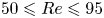 $50 \leqslant Re \leqslant 95$. A stabilized finite element formulation based on streamline-upwind/Petrov–Galerkin (SUPG) and pressure-stabilizing/Petrov–Galerkin (PSPG) stabilizing techniques (Tezduyar et al. Reference Tezduyar, Mittal, Ray and Shih1992) is utilized to solve the Navier–Stokes equations for an incompressible flow. It has been shown earlier (e.g. Behara & Mittal Reference Behara and Mittal2010b) that the oblique shedding angle depends on the boundary layer thickness (
 $\delta$) of the incoming flow at the cylinder ends. To this extent, the length of the side wall upstream of the cylinder, for each simulation in the present study, is prescribed so that
  $\delta$ is the same for all cases. A broad classification of the flows in various regimes in the
  $AR$–
$AR$– $\textit {Re}$ plane is proposed based on the number of cells, nature and angle of oblique vortices, nature of dislocations and end cell structure.
To explore the reason for the appearance of different number of cells for various combinations of  $AR$ and
  $\textit {Re}$, global linear stability analysis of the flow equations (Theofilis Reference Theofilis2011) is carried out. Linear stability analysis has been successfully applied in the past to understand instabilities in several flows. For example, it has been used to determine the unstable modes of flow as well as the critical
  $\textit {Re}$ for the onset of the instability of the wake of a circular cylinder (Jackson Reference Jackson1987; Barkley & Henderson Reference Barkley and Henderson1996; Ding & Kawahara Reference Ding and Kawahara1998; Mittal & Kumar Reference Mittal and Kumar2003; Kumar et al. Reference Kumar, Kottaram, Singh and Mittal2009). In the present work, global linear stability analysis of the steady flow is conducted for two sets of disturbances. In the first case, the disturbance is assumed to be periodic along the span. Such an analysis is often referred to as a biglobal linear stability analysis (Theofilis Reference Theofilis2011; Mittal, Sidharth & Verma Reference Mittal, Sidharth and Verma2014; Mittal & Dwivedi Reference Mittal and Dwivedi2017). This is followed up with the analysis for a general disturbance field: the triglobal linear stability analysis (Theofilis Reference Theofilis2011). The time evolution of the flow initiated from the steady flow superimposed with the unstable eigenmodes, from the linear stability analysis, is carried out to further understand the role of nonlinear effects in the formation of cells along the span of the cylinder.
2. The governing equations and their finite element formulation
2.1. The incompressible flow equations
Let  $\boldsymbol {\varOmega } \subset \mathbb {R} ^{n_{sd}}$ and
  $(0,T)$ be the spatial and temporal domains, respectively, where
  $n_{sd}$ is the number of space dimensions and let
  $\varGamma$ denote the boundary of
  $\varOmega$. The spatial and temporal coordinates are denoted by
  $\boldsymbol {x}$ and
  $t$. The equations that govern the incompressible flow of fluid are
 \begin{gather} \rho \left(\frac{\partial \boldsymbol{u}}{\partial t} + \boldsymbol{u} \boldsymbol{\cdot} \boldsymbol{\nabla} \boldsymbol{u} \right) - \boldsymbol{\nabla} \boldsymbol{\cdot} \boldsymbol{\sigma} = \mathbf{0} \quad \textrm{on} \ \varOmega \times \left( 0,T\right), \end{gather}
 \begin{gather}\boldsymbol{\nabla} \boldsymbol{\cdot} \boldsymbol{u} = 0 \quad \textrm{on} \ \varOmega \times \left( 0,T \right). \end{gather}
Here  $\rho$,
  $\boldsymbol {u}$ and
  $\boldsymbol {\sigma }$ are the density, velocity and stress tensor, respectively. For a Newtonian fluid, the stress tensor is
 \begin{equation} \boldsymbol{\sigma} ={-} p {\boldsymbol{\mathsf{I}}}+ {\boldsymbol{\mathsf{T}}}, \quad {\boldsymbol{\mathsf{T}}} = 2 \mu \boldsymbol{\varepsilon} \left(\boldsymbol{u}\right), \quad \boldsymbol{\varepsilon} \left(\boldsymbol{u}\right) = \tfrac{1}{2} [(\boldsymbol{\nabla} \boldsymbol{u}) + (\boldsymbol{\nabla} \boldsymbol{u})^{\textrm{T}}], \end{equation}
where  $p$,
$p$,  ${\boldsymbol{\mathsf{I}}}$ and
  $\mu$ are the pressure, identity tensor and dynamic viscosity, respectively. The associated boundary conditions used for solving (2.1) and (2.2) are described in § 3.2. The initial condition for the simulation of each case of
  $AR$ and
  $\textit {Re}$ is the corresponding steady flow. It is computed by simply dropping the unsteady term from (2.1). We denote the steady flow by
  $(\boldsymbol {U}, {P})$, where
  $\boldsymbol {U}$ is the velocity and
  ${P}$ is the pressure field.
A stabilized finite element formulation is utilized to solve the governing flow equations in the primitive variable form. The details of the formulation can be found in our earlier work (Mittal Reference Mittal2000, Reference Mittal2001; Behara & Mittal Reference Behara and Mittal2009). The terms that provide numerical stabilization to the computations are based on the SUPG and PSPG stabilizing techniques (Tezduyar et al. Reference Tezduyar, Mittal, Ray and Shih1992). The finite element discretization results in nonlinear equations which are solved using the generalized minimal residual (GMRES) technique (Saad & Schultz Reference Saad and Schultz1986) in conjunction with diagonal preconditioners.
2.2. The linear stability flow equations
The unsteady flow,  $(\boldsymbol {u}, p )$, is expressed as a combination of the steady flow
  $(\boldsymbol {U}, {P})$ and disturbance
  $(\boldsymbol {u'}, {p'})$:
  $\boldsymbol {u} = \boldsymbol {U} + \boldsymbol {u'}$ and
  $p = P + p'$. Here
  $\boldsymbol {u'}$ and
  $p'$ are the disturbance fields of the velocity and pressure, respectively. For small disturbance, the linearized equations for the time evolution of the disturbance fields are
 \begin{gather} \rho \left(\frac{\partial \boldsymbol{u}'}{\partial t} + \boldsymbol{u}' \boldsymbol{\cdot} \boldsymbol{\nabla} \boldsymbol{U} + \boldsymbol{U} \boldsymbol{\cdot} \boldsymbol{\nabla} \boldsymbol{u}' \right) - \boldsymbol{\nabla} \boldsymbol{\cdot} \boldsymbol{\sigma}' = \mathbf{0} \quad \textrm{on} \ \varOmega \times \left(0,T\right), \end{gather}
 \begin{gather}\boldsymbol{\nabla} \boldsymbol{\cdot} \boldsymbol{u}' = 0 \quad \textrm{on} \ \varOmega \times \left( 0,T \right). \end{gather}
Here  $\boldsymbol {\sigma }'$ is the stress tensor for the disturbance field
  $(\boldsymbol {u}', p' )$. More details on these equations can be found in the article by Mittal et al. (Reference Mittal, Sidharth and Verma2014). Two sets of disturbances are considered. In the first case, the disturbance is assumed to be periodic along the span. Let
  $\lambda _{z}$ denote the spanwise wavelength of the disturbance. The corresponding wavenumber is
  $\beta \ ({=}2 {\rm \pi} /\lambda _{z})$. No assumption is made on the spatial distribution of the disturbance in the
  $xy$ plane. However, it is assumed to be associated with a global temporal frequency as well as a rate of growth/decay that is spatially invariant. Such a disturbance is represented as
 \begin{equation} \boldsymbol{u}'\left(x,y,z,t\right) = \hat{\boldsymbol{u}} \left( x,y \right) \textrm{e}^{ \textrm{i} \beta z} \,\textrm{e}^{\lambda t}, \quad p' \left( x,y,z,t \right) = \hat{p} \left( x,y \right) \textrm{e}^{ \textrm{i} \beta z}\,\textrm{e}^{\lambda t}. \end{equation}
The analysis with a disturbance of this form is often referred to as a biglobal linear stability analysis (Theofilis Reference Theofilis2011; Mittal et al. Reference Mittal, Sidharth and Verma2014; Mittal & Dwivedi Reference Mittal and Dwivedi2017). It is repeated for several values of  $\beta$ to determine the mode with the largest growth rate.
Linear stability analysis is also carried out for a more general disturbance that does not assume periodicity along the span. However, the global nature of the time frequency and rate of growth/decay, that are spatially invariant, is retained. This constitutes the second form of the disturbance being considered and can be represented as
 \begin{equation} \boldsymbol{u}'\left(x,y,z,t\right) = \hat{\boldsymbol{u}} \left( x,y,z \right) \textrm{e}^{\lambda t}, \quad p' \left( x,y,z,t \right) = \hat{p} \left( x,y,z \right) \textrm{e}^{\lambda t}. \end{equation}
The analysis for this general disturbance field is referred to as the triglobal linear stability analysis (Theofilis Reference Theofilis2011). It is more expensive than the biglobal analysis. In both analyses,  $\lambda$ is the eigenvalue of the fluid system and governs the stability of the base flow,
  $({\boldsymbol {U}}, P )$. In general,
  $\lambda$ is complex and can be represented as
  $\lambda =\lambda _{r}+\textrm {i}\lambda _{i}$ where
  $\lambda _{r}$ and
  $\lambda _{i}$ are the real and imaginary parts, respectively. Here
  $\lambda _{i}$ represents the oscillation frequency of the corresponding mode of perturbation whereas
  $\lambda _{r}$ represents the growth rate; a positive
  $\lambda _{r}$ leads to instability.
The finite element formulation to carry out a biglobal linear stability analysis can be found in our earlier work (Mittal & Kumar Reference Mittal and Kumar2003; Mittal et al. Reference Mittal, Sidharth and Verma2014; Mittal & Dwivedi Reference Mittal and Dwivedi2017). Mittal & Kumar (Reference Mittal and Kumar2003) presented the formulation as well as the analysis in two dimensions. These formulations have been used in our earlier studies to investigate the circular Couette flow (Mittal et al. Reference Mittal, Sidharth and Verma2014) and flow past stationary and rotating circular cylinders (Mittal & Kumar Reference Mittal and Kumar2003; Kumar & Mittal Reference Kumar and Mittal2006; Kumar et al. Reference Kumar, Kottaram, Singh and Mittal2009; Mittal et al. Reference Mittal, Sidharth and Verma2014). The extension to three dimensions, for the triglobal linear stability analysis, is a straightforward generalization.
The finite element formulation for the global linear stability analysis leads to a generalized eigenvalue problem of the form  $\boldsymbol{\mathsf{A}} X - \lambda \boldsymbol{\mathsf{B}} X = 0$, where
  $\boldsymbol{\mathsf{A}}$ and
  $\boldsymbol{\mathsf{B}}$ are non-symmetric matrices. Various algorithms have been developed in the past to solve such eigenvalue problems with large sparse non-symmetric matrices (Wilkinson Reference Wilkinson1965; Stewart Reference Stewart1976; Meyer Reference Meyer1987). The matrix
  $\boldsymbol{\mathsf{B}}$, in the present case, is singular owing to the nature of the continuity equation that is used to determine pressure. This is circumvented by solving for the inverse problem, i.e. eigenvalues for
  $\boldsymbol{\mathsf{B}} X - ({1}/{\lambda }) \boldsymbol{\mathsf{A}} X = 0$ are computed. To check the stability of the steady-state solution, we locate the rightmost eigenvalue (eigenvalue with largest real part) using the subspace iteration method (Stewart Reference Stewart1975).
3. Problem description
3.1. Computational domain
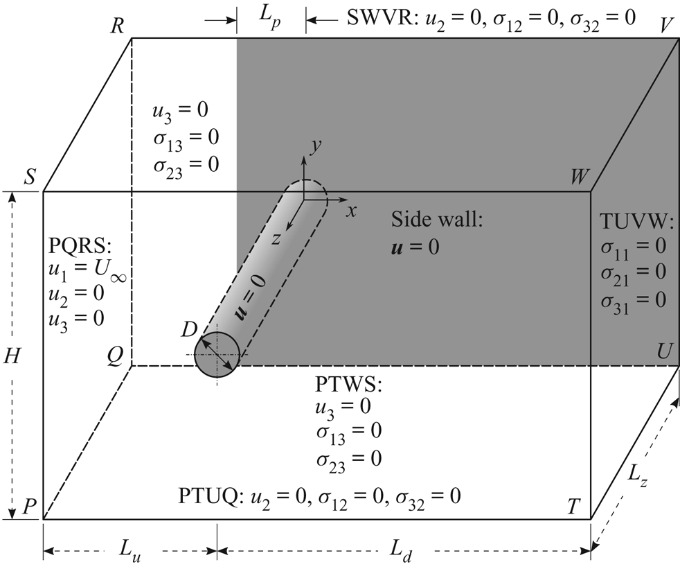
A schematic of the problem set-up and the computational domain is shown in figure 1. A cylinder, of diameter  $D$, is placed in a rectangular computational domain whose upstream and downstream boundaries are located at a distance of
  $L_{u}$ and
  $L_{d}$, respectively, from the centre of the cylinder. The height of the domain is
  $H$. The cylinder occupies the entire span,
  $L_{z}$, of the domain. To reduce the requirement of computational resources we take advantage of the geometric symmetry and simulate only one half of the span. The solution from half the span is reflected along the mid-span to generate the flow for the entire span and computations, for a few cases, are continued with the full span. It is found that in most cases the symmetry of the flow about the mid-span is retained. The flow loses symmetry for some of the cases corresponding to two and four cells in half the span. Details of these computations are presented later in the paper. We recall that the aspect ratio of the cylinder is defined as
  $AR=L/D$. The span of the computational domain,
  $L_{z}$, is
  $L/2$. The face PTWS is the plane of symmetry, whereas the face QUVR is the ‘end wall’. A section of this plane is utilized to model the effect of ‘end plates’. The ‘side wall’ that simulates this effect is highlighted in figure 1 via shading. The free-stream velocity is along the
  $x$-axis, whereas the axis of the cylinder is along the
  $z$-axis. The origin of the coordinate system coincides with the centre of the cylinder at the face QUVR. The effect of the location of upstream and downstream boundaries and the height of the domain has been studied in detail in an earlier work by Prasanth & Mittal (Reference Prasanth and Mittal2008) for two-dimensional computations past a freely vibrating cylinder. It was reported that a computational domain with
  $L_{u}=15D$,
  $L_{d}=25.5D$ and
  $H=40D$ is large enough to eliminate any significant effect of the size. The present computations have been carried out with an even larger domain with
  $L_{u}=27.5D$,
  $L_{d}=50D$ and
  $H=100D$. The blockage ratio (
 $D/H$) is
  $1\,\%$ for the present study.

Figure 1. Flow past a cylinder with side wall: schematic of the computational domain and the associated boundary conditions. The sketch is not to scale.
3.2. Boundary conditions
The boundary conditions are shown in figure 1. Uniform flow is prescribed on the upstream face PQRS whereas the stress vector is set to zero at the outflow face TUVW. The symmetry condition is prescribed on all other walls of the computational domain, i.e. the velocity component normal to the wall, and the stress vector components in the plane of the wall are set to zero. No-slip boundary condition is specified on the cylinder surface and the side wall on QUVR for  $x\geqslant -L_{p}$. These conditions are similar to those used by Behara & Mittal (Reference Behara and Mittal2010b). For the linear stability analysis, the boundary conditions are the homogeneous version of those used for direct numerical simulations.
3.3. The parameters
The three main parameters that affect the flow being studied are  $\textit {Re}$,
  $AR$ and
  $\delta$. The Reynolds number is defined as
  $\textit {Re} = U_{\infty } D/ \nu$, where
  $U_{\infty }$ is the free stream speed,
  $D$ the diameter of the cylinder and
  $\nu$ the kinematic viscosity of the fluid. Computations are carried out for
  $50 \leqslant \textit {Re} \leqslant 95$. The range of aspect ratio of the cylinder considered in the present study is
  $5 \leqslant AR \leqslant 90$. The flow is also affected by the thickness of the boundary layer (
 $\delta$) on the side wall as it approaches the cylinder. In turn,
  $\delta$ depends on
  $Re$ and the extent of the side wall upstream of the cylinder (
 $L_{p}$, as shown in figure 1). All the computations in the present work are carried out by suitably adjusting
  $L_{p}$ so that
  $\delta$ is
  $2D$ at
  $x=0$. With
  $\delta$ being held constant, the flow depends on only two parameters:
  $AR$ and
  $\textit {Re}$. For brevity, we introduce the notation
  $(AR, \textit {Re})$ to refer to the set of independent parameters that govern the flow in this study.
3.4. Finite element mesh
First, a two-dimensional mesh is generated around the circular cylinder. It is sufficiently refined near the surface of the cylinder to resolve the boundary layer, its spatial evolution and its separation. The mesh and its close-up view near the cylinder is shown in figure 2. It has 140 elements along the circumferential direction and the height of the first element on the surface of the cylinder surface is  $0.003D$. The three-dimensional mesh is obtained by stacking several slices of the two-dimensional mesh along the span. The distribution of the grid points along the span is not uniform. The spanwise resolution near the side wall is finer to resolve the boundary layer that forms on it. The thickness of the element on the surface of the side wall is
  $0.05D$. The three-dimensional mesh for a cylinder of
  $AR=60$ is obtained by stacking
  $n_{z}=100$ slices of the two-dimensional mesh along the span. For other
  $AR$,
$AR$,  $n_{z}$ is suitably chosen to maintain the same spatial resolution.
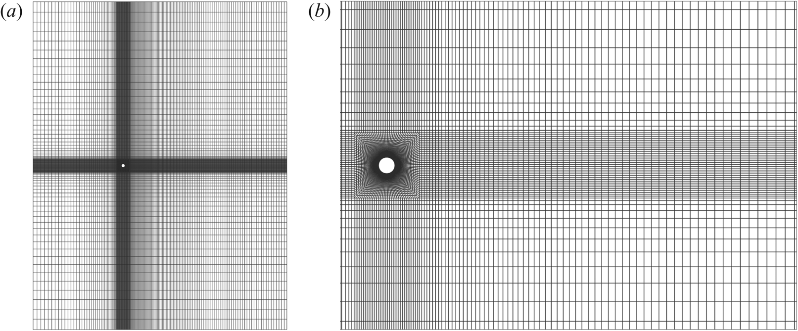
Figure 2. Flow past a cylinder with side wall: (a) two-dimensional section of the finite element mesh M3, listed in table 1, in the  $xy$ plane; (b) enlarged view of the mesh near the cylinder.
Four meshes are utilized to investigate the adequacy of spatial resolution. The study is carried for the case of  $(AR, \textit {Re})=(60, 60)$. In the
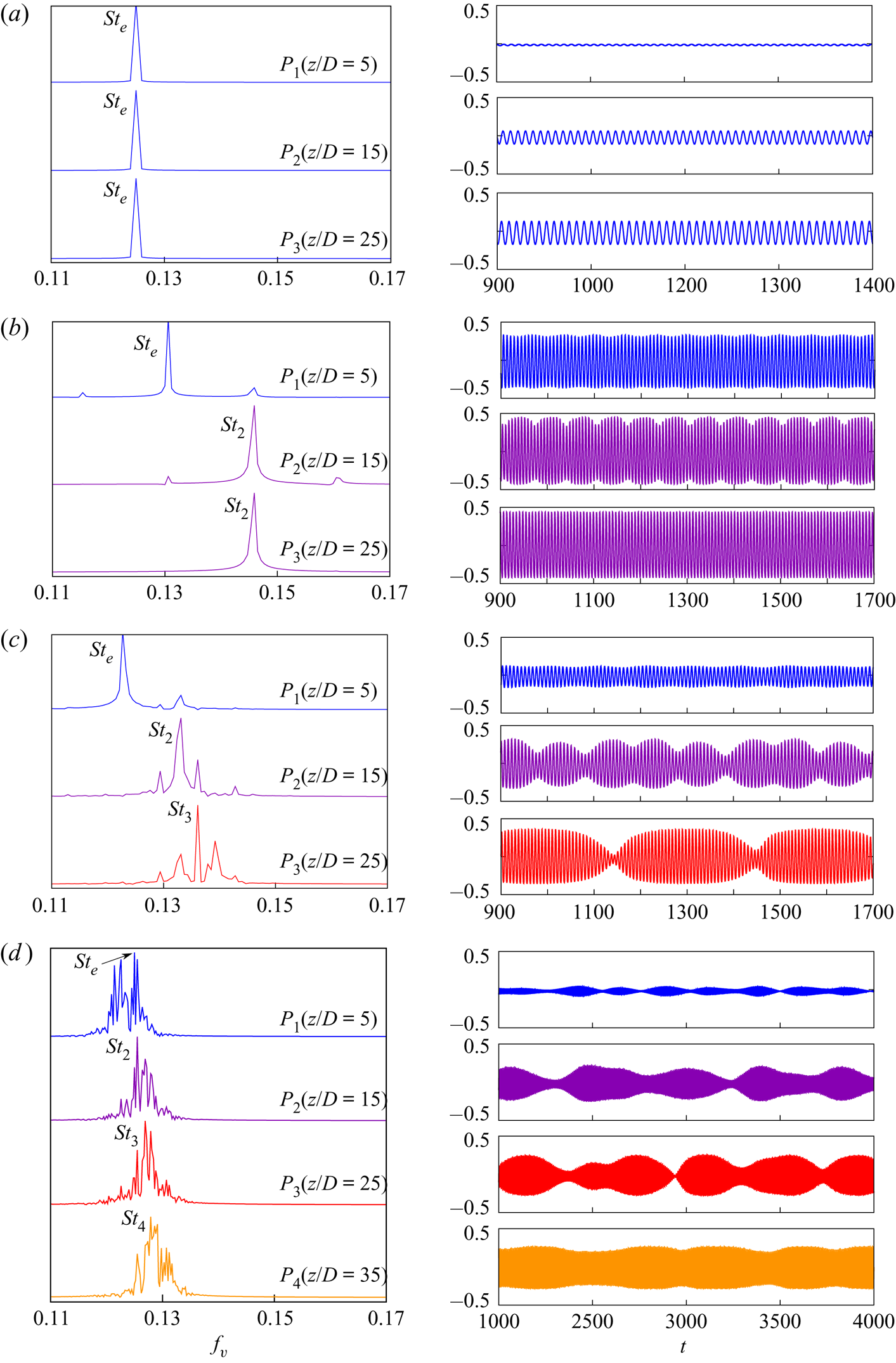
  $xy$ plane, each two-dimensional section of the mesh M1 consists of 5242 nodes and 5077 quadrilateral elements. The numbers are 13 728 and 13 460 for mesh M2, 21 500 and 21 164 for mesh M3 and 30 860 and 30 456 for mesh M4, respectively. The spatial extent of the computational domain of all four meshes is identical. The number of elements along the span for the meshes M1–M4 are 50, 80, 100 and 120, respectively. The time-averaged and r.m.s. values of the aerodynamic force coefficients for the four meshes are presented in table 1. Results from all meshes are in good agreement with respect to the mean and r.m.s. values of drag coefficients. The only significant deviation is in the r.m.s. value of lift coefficient obtained from mesh M1. Mesh M3 has excellent agreement with all the parameters of mesh M4. This demonstrates the adequacy of the spatial resolution of mesh M3, and is utilized for all computations in this work. A time step of
  $\Delta t=0.1$ is used for all the computations except for the time evolution of unstable modes obtained from linear stability analysis, which utilize an even smaller time step of
  $\Delta t=0.01$.
Table 1. Flow past a cylinder with side wall: details of the various finite element meshes. Also listed are the time-average and r.m.s. value of the force coefficients for the fully developed unsteady flow corresponding to  $(AR, \textit {Re})=(60,60)$.

4. Results
4.1. Cellular structure of the wake
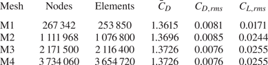
Cellular shedding is a distinct feature of the wake of a wall-bounded cylinder and has been observed in the past in experimental and numerical studies (Williamson Reference Williamson1989; König et al. Reference König, Eisenlohr and Eckelmann1990; Behara & Mittal Reference Behara and Mittal2010b). The vortex shedding frequency across the span, in a cell, is uniform. Figure 3 shows a map of the number of cells observed in the present computations on the  $(AR, \textit {Re})$ plane. The flow is steady for low
  $AR$ for all the
  $\textit {Re}$ considered. The critical
  $\textit {Re}$ for the onset of vortex shedding decreases with increase in
  $AR$. For example, the flow is steady even at
  $\textit {Re}=95$ for
  $AR=5$. In comparison, the flow is unsteady at
  $\textit {Re}=50$ for
  $AR=20$. In general, each
  $\textit {Re}$ is associated with two values of critical
  $AR$:
$AR$:  $AR_{{cr}_{1}}$ and
  $AR_{{cr}_{2}}$. The flow is steady for
  $AR < AR_{{cr}_{1}}$. It is unsteady for
  $AR\geqslant AR_{{cr}_{1}}$ and associated with a single cell for
  $AR\leqslant AR_{{cr}_{2}}$. For
  $AR>AR_{{cr}_{2}}$, the flow may be associated with either two or three or four cells, depending on the
  $AR$ and
  $\textit {Re}$. We recall the results reported from earlier experimental studies with large
  $AR$ cylinders, where three cell shedding is observed for
  $\textit {Re}<64$ and two cells for larger
  $\textit {Re}$ (Williamson Reference Williamson1989). The present study reveals the rich flow structure for low
  $AR$ cylinders. Cells can be identified from the spanwise variation of either the vortex structures or vortex shedding frequency.

Figure 3. Flow past a cylinder with side wall: cellular structures in the wake for cylinders of  $5 \leqslant AR \leqslant 90$ and
  $50 \leqslant \textit {Re} \leqslant 95$. The boundaries of the regions attributed to the respective flow structures are not exact, but indicative in nature and are based on the cases for which computations have been carried out and marked by hollow symbols. More details for the flow are given in figure 4 for the parameters indicated by solid symbols. The hatched region indicates the range of parameters where the flow loses symmetry about the mid-span of the cylinder. The range of
  $\textit {Re}$ along the
  $x$-axis is 49–96.
Several methods have been proposed in the past to identify the vortex cores and their region of influence (Zhang et al. Reference Zhang, Liu, Xian and Du2018). The  $Q$-criterion proposed by Hunt, Wray & Moin (Reference Hunt, Wray and Moin1988) and
  $\lambda _2$-criterion by Jeong & Hussain (Reference Jeong and Hussain1995) are most widely used. Liu et al. (Reference Liu, Wang, Yang and Duan2016) proposed the
  $\varOmega$ method for vortex identification. A brief description of the
  $Q$,
$Q$,  $\lambda _2$ and
  $\varOmega$ criteria and comparison of the flow structures obtained using them is presented in Appendix A. It is found that, for the present class of flows, all the three criteria result in virtually identical flow structures. The
  $Q$-criterion is used to identify the vortex structures in this work.
A typical case of each of the flow regimes with respect to the number of cells across the span is shown in figure 4. The flow with one cell (figure 4a) is the simplest case. It has also been observed in experiments, for example, by Albarède & Provansal (Reference Albarède and Provansal1995). For flows with multiple cells, vortex dislocations appear periodically at the boundaries of adjacent cells. The cell closest to the side wall is named as the end cell. The subsequent cells, as one moves away from the wall and towards the centre-span, are named as the second, third and fourth cell, respectively. It is interesting to note that the cell near the mid-span is largest for the two-cell case whereas that is not true for the cases with three and four cells. The vortex dislocation appearing at the junction of the end cell and the second cell is referred to as  $D_{1}$. That between the second cell and third cell is named
  $D_{2}$. Similarly, the dislocation at the junction of the third and fourth cell is referred to as
  $D_{3}$. The dislocation
  $D_{2}$ that divides the second and third cell, for the case of four cells, is not shown in figure 4(d). It is presented in later in the paper for the simulation with full span at three time instants to show all the dislocations. The oblique angle at which the vortices are inclined to the cylinder axis is found to be the largest in the end cell in accordance with the observations of König et al. (Reference König, Eisenlohr and Eckelmann1992). It decreases as one moves towards the second, third and fourth cell, respectively. Also shown in figure 4 is the spanwise variation of the non-dimensional vortex shedding frequency corresponding to the dominant frequency in the time histories of the cross-flow component of velocity.
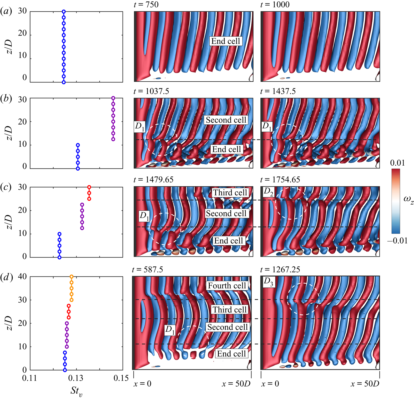
Figure 4. Flow past a cylinder with side wall: spanwise variation of Strouhal number corresponding to the dominant frequency of vortex shedding and  $xz$-view of instantaneous
  $Q$ (
$Q$ ( ${=}0.0002$) iso-surface coloured with spanwise vorticity component at different time instants for (a)
  $(AR, \textit {Re})=(60, 50)$, (b)
  $(AR, \textit {Re})=(60, 75)$, (c)
  $(AR, \textit {Re})=(60, 60)$ and (d)
  $(AR, \textit {Re})=(80, 54)$. The various cells and the vortex dislocations are marked. The broken lines show the indicative cell boundaries based on the vortex dislocations. All subsequent
  $Q$ iso-surfaces are coloured following the same convention as in this figure.
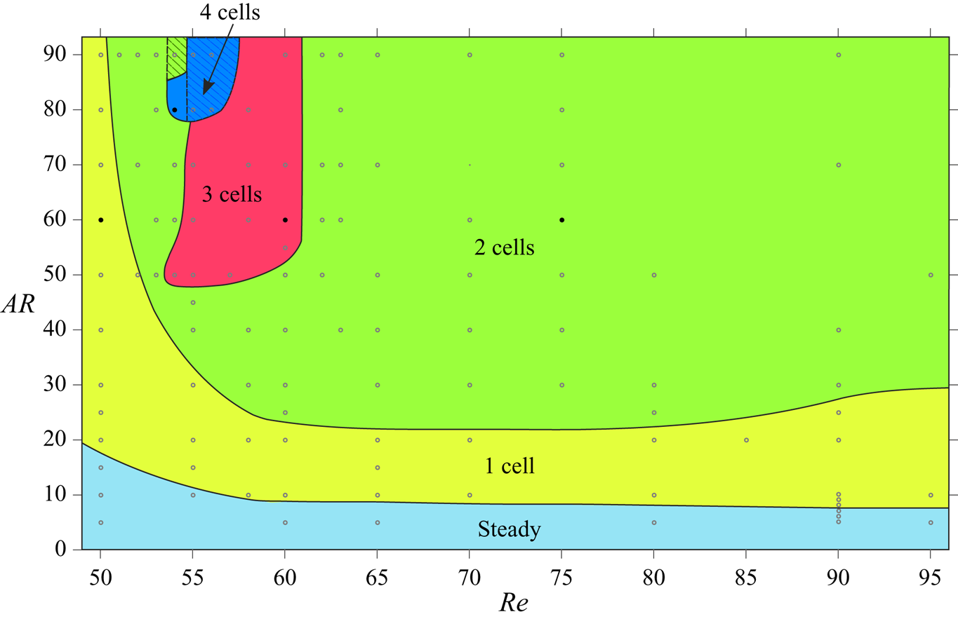
Figure 5 presents the frequency spectra of time histories of cross-flow velocity component at spanwise separated locations for the cases shown in figure 4. The probe  $P_{1}$ is located at
  $z/D=5$ and successive probes
  $P_{2}$,
  $P_{3}$ and
  $P_{4}$ (where applicable) are
  $10D$ apart along the span. They are all located in the near wake (
 $x/D=5,\ y/D=0.25$). For the single-cell case, all probes record the end cell frequency of
  $St_{e}=0.125$. For the two-cell case, the probe
  $P_{1}$ reports the end cell frequency and probes
  $P_{2}$ and
  $P_{3}$ report the second cell frequency. The peaks correspond to values
  $St_{e}=0.1306$ and
  $St_{2}=0.1459$. For the three-cell case, the probes
  $P_{1}$,
  $P_{2}$ and
  $P_{3}$ record the shedding frequencies at the end cell, second cell and third cell, with the peak values being
  $St_{e}=0.1227$,
  $St_{2}=0.1331$ and
  $St_{3}=0.1361$. For the four-cell case, the probes
  $P_{1}$,
  $P_{2}$,
  $P_{3}$ and
  $P_{4}$ report the shedding frequencies at the end cell, second cell, third cell and fourth cell, respectively. The Strouhal numbers corresponding to the peaks in each cell are
  $St_{e}=0.1250$,
  $St_{2}=0.1260$,
  $St_{3}=0.1269$ and
  $St_{4}=0.1279$. The shedding frequency is found to increase from the end cell towards the fourth cell. It was shown by Williamson (Reference Williamson1989), and later Behara & Mittal (Reference Behara and Mittal2010b), that the low-frequency modulation in the time histories in figure 5(b–d) are due to the appearance of vortex dislocations in the wake. This is discussed in more detail later in the paper.

Figure 5. Flow past a cylinder with side wall: cross-flow component of velocity ( $v$), and their corresponding power spectra at spanwise separated probe locations for (a)
  $(AR, \textit {Re})=(60, 50)$, (b)
  $(AR, \textit {Re})=(60, 75)$, (c)
  $(AR, \textit {Re})=(60, 60)$ and (d)
  $(AR, \textit {Re})=(80, 54)$. The probes are located at (
 $x/D=5, y/D=0.25$), and
  $z/D$ as mentioned in the figure. The amplitude of the power spectra has been normalized by the maximum value of each case.
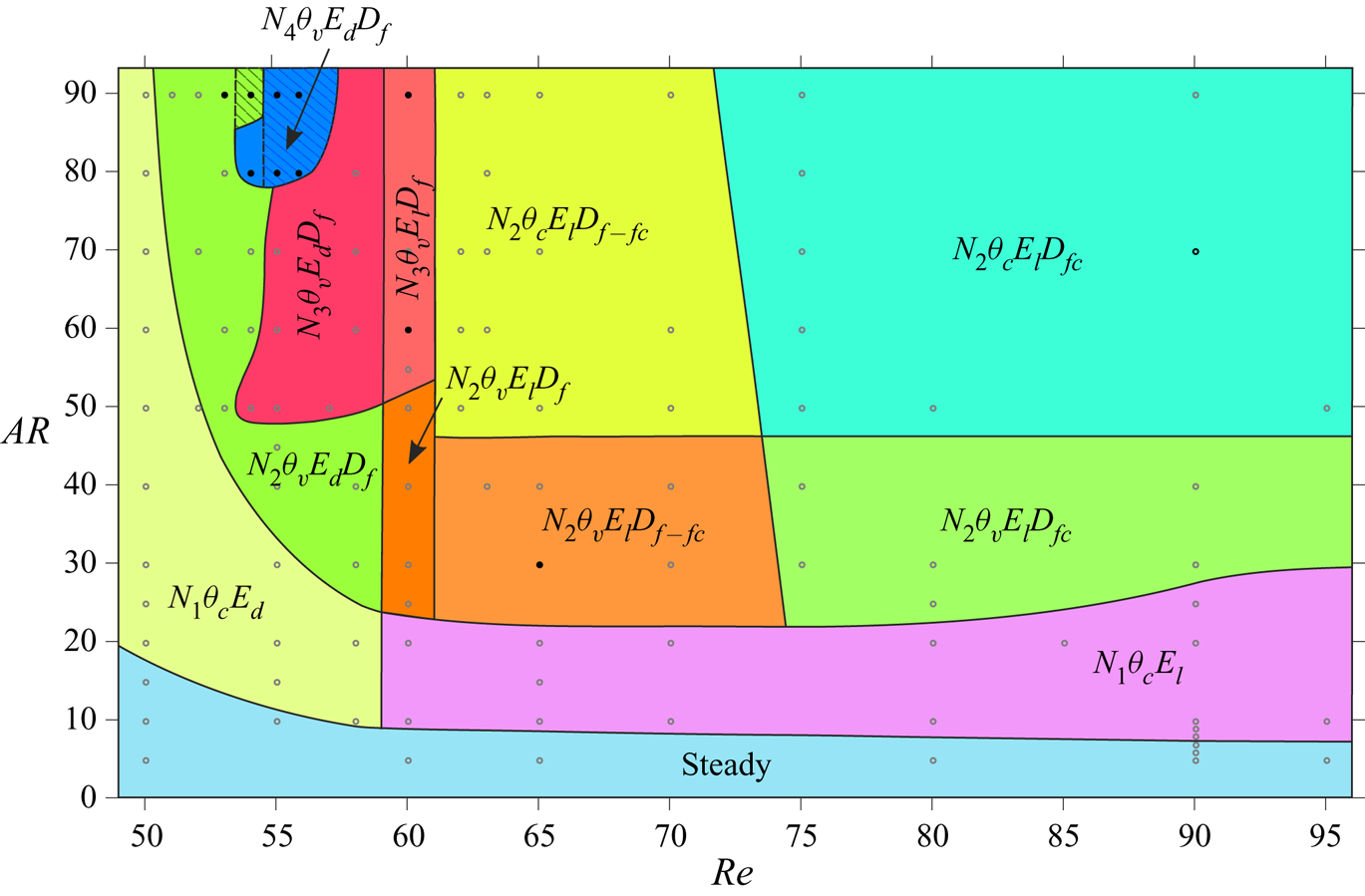
4.2. Flow characterization
A number of interesting features are observed in the wake. The various attributes of the flow that are considered in this study are the number of cells along the span ( $N_{n}$), the oblique angle that the vortices make with the axis of the cylinder (
 $\theta$), the structure of the vortices near the side wall (
 $E$) and the nature of vortex dislocations between the various cells (
 $D$). We note that the number of cells along the full span is
  $2n-1$. Based on these attributes, we broadly classify the flow in certain regimes in the
  $AR\text {--}\textit {Re}$ plane. Table 2 lists the various states that these attributes exhibit. For example, the flow in regime
  $N_{4}\theta _{v}E_{d}D_{f}$ consists of four cells along half the span, the oblique angle of the vortices varies along the span and with time, the vortices diffuse close to the side wall and the vortex dislocation is of the fork type. Similarly,
  $N_{2}\theta _{c}E_{l}D_{fc}$ signifies that the wake is associated with two cells along half the span, the oblique angle of the vortices remains constant along the span and with time, the vortices of opposite signs with respect to spanwise vorticity are linked close to the side wall and the vortex dislocation is of the connected fork type. The classification based on these features is presented in figure 6. The boundaries of the various regimes are indicative extents in which similar attributes can be observed in the wake. The number of cells along half the span (
 $N_{n}$) that can occur in the flow are shown in figure 4 and described in § 4.1. For several cases in the
  $AR$–
$AR$– $Re$ plane, the flow computed with symmetry condition along the half-span of the cylinder was reflected about the centre-line and computations continued with the full domain without imposition of symmetry. In most cases, the flow retained its symmetry. The hatched region in figures 3 and 6 indicate the regime for which the flow loses symmetry. However, it retains all the attributes of the flow constrained to be symmetric about mid-span. Details of these cases are presented later in the paper. The other attributes that describe the regimes in the
  $AR\text {--}Re$ plane are discussed in the following.

Figure 6. Flow past a cylinder with side wall: classification of the flow in the  $AR$–
$AR$– $\textit {Re}$ plane on the basis of the attributes defined in table 2. The boundaries of the various regions are not exact, but indicative in nature and are based on the cases for which computations have been carried out and marked by hollow symbols. The cases for which a full-span simulation is initiated from the solution from half-span, by reflecting it about mid-span, are highlighted using solid symbols. The lower and upper limit along the
  $x$-axis is
  $49$ and
  $96$, respectively.
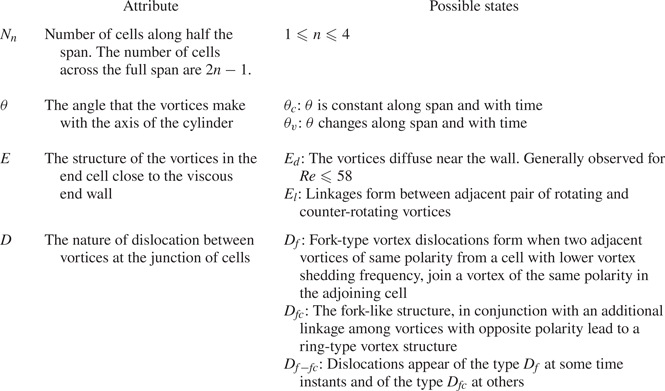
Table 2. Flow past a cylinder with side wall: the nomenclature adopted to define the attributes of the flow.

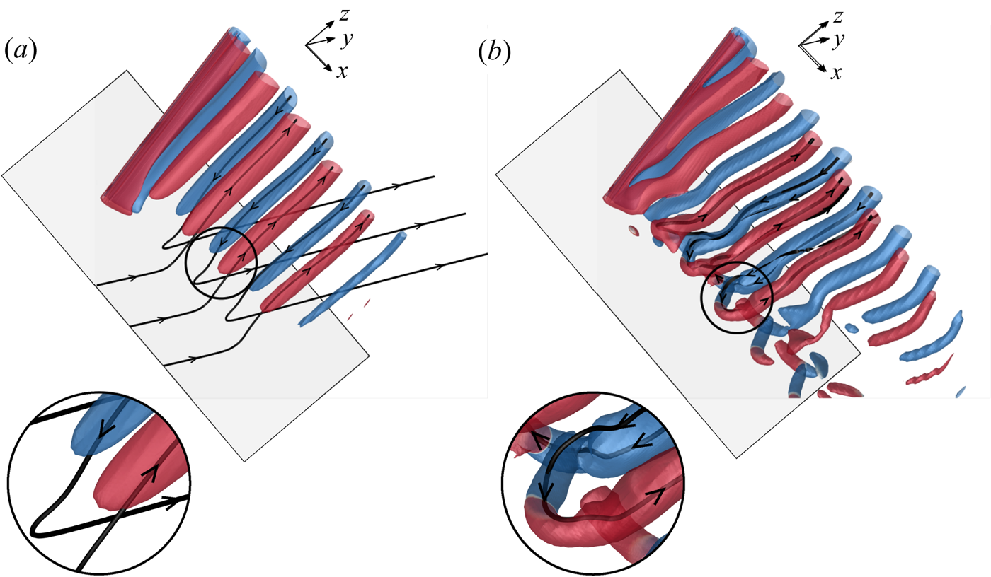
4.2.1. End vortex structures
The topology of the vortices near the side wall depends on  $(AR, \textit {Re})$. Two type of end vortex structures have been identified: the diffused type and linked type. They are represented by
  $E_{d/l}$, where the subscripts ‘
 $d$’ and ‘
 $l$’ indicate diffused and linked type, respectively. Their existence for different combinations of
  $(AR, \textit {Re})$ are presented in figure 6. Figure 7 illustrates the two types of end vortex structures via the iso-
 $Q$ surfaces. Also shown in the figure are a few vortex lines that pass through the core of the vortices at the plane of symmetry. Figure 7(a) shows the diffused end vortex structure wherein the spanwise vortices appear to diffuse near the side wall. Interestingly, the vortex lines from the spanwise vortices connect to those within the boundary layer that forms on the side wall. Diffused-type end vortex structures are generally found for
  $\textit {Re}\leqslant 58$. Linkages form between adjacent pair of rotating and counter-rotating vortices near the side wall for larger
  $\textit {Re}$. Figure 7(b) shows a case of linked-type end vortex structure. Unlike in the case of diffused end vortex structure, the vortex lines emerging from the vortices of opposite polarity connect to form a closed loop. A similar model of braided vortices at the ends was suggested by Eisenlohr & Eckelmann (Reference Eisenlohr and Eckelmann1989). Figure 7(a) was reconstructed for even lower values of
  $Q$ to specifically check if the diffused end vortex structures might show linkages with neighbouring vortices. It is found that the end vortices retain their structure.

Figure 7. Flow past a cylinder with side wall:  $Q$ (
$Q$ ( ${=}0.002$) iso-surfaces coloured with spanwise component of vorticity (
 $\omega _z = \pm 0.01$) for the instantaneous flow depicting (a) diffused end vortex structures for
  $(AR, \textit {Re})= (60, 50)$ at
  $t=1350$ and (b) linked end vortex structures for
  $(AR, \textit {Re})=(60, 75)$ at
  $t=1725$. Also shown are a few vortex lines for each case that pass through the core of the vortices at the plane of symmetry and the enlarged view of the images next to the side wall. The side wall (
 $z=0$) is shown for reference.
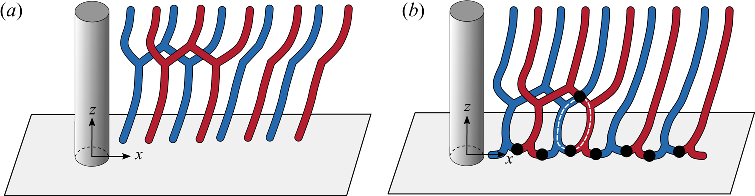
4.2.2. Vortex dislocations
Vortex dislocations appear at the boundaries between adjacent cells. Based on their topology, they may be broadly classified in two categories: fork type and connected fork type. A mixed type has also been observed in some cases. As listed in table 2, the dislocations are represented as  $D_{f/f-fc/fc}$, where the subscripts ‘
 $f$’, ‘
 $f-fc$’ and ‘
 $fc$’ represent fork-type, mixed-type and connected fork-type. Fork-type dislocations occur when two adjacent vortices of the same polarity from a cell with lower vortex shedding frequency join a vortex of the same polarity in the adjoining cell. Figure 8(a) shows a schematic. A similar model was proposed by Williamson (Reference Williamson1989). The fork-like connections made by the anti-clockwise and clockwise rotating vortices of two adjacent cells, for the (
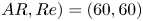 $AR, Re)=(60, 60)$ case, are highlighted in figures 9(a) and 9(b), respectively. Both images are for the flow at the same time instant, but viewed from different
  $y$ locations to bring out the details of the flow structure. In some cases it is observed that along with fork-like structures, two vortices with opposite polarity form an additional linkage at the cell boundary. This leads to the formation of a ring-like vortex structure. We refer to these as connected fork-type vortex dislocations (
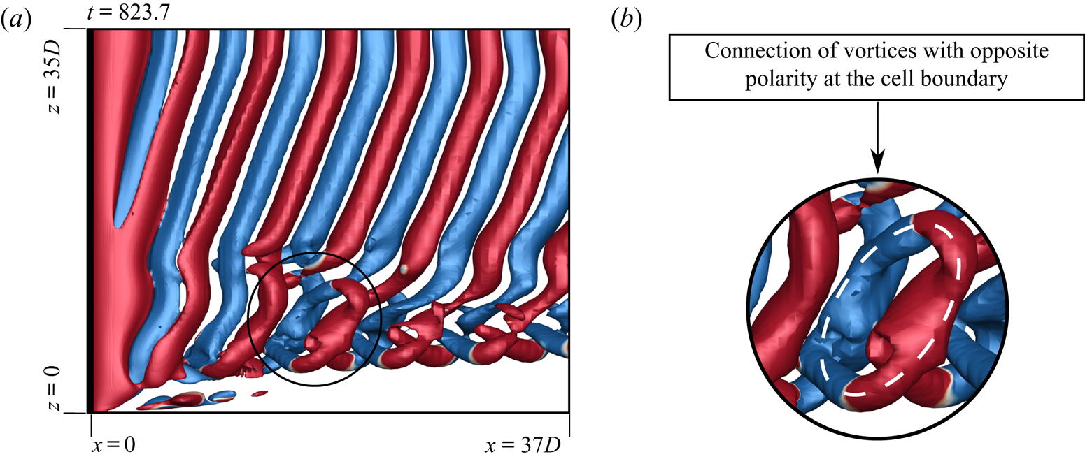
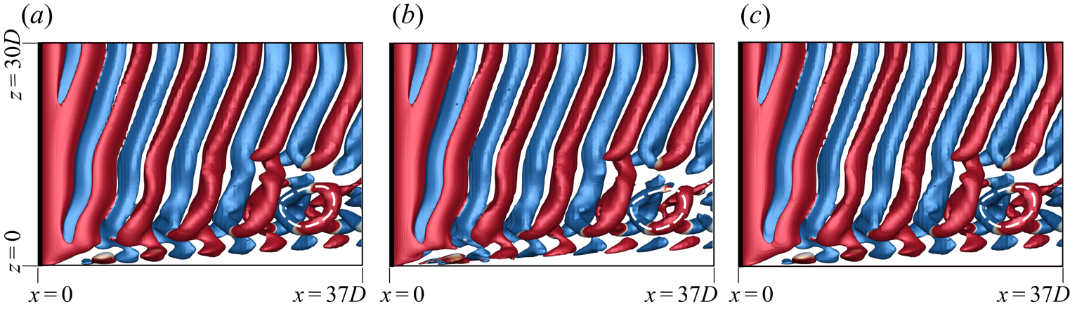
 $D_{fc}$). The schematic of the connected fork-type dislocation is presented in figure 8(b). Connected fork-type vortex dislocations are observed only in those cases that exhibit linked-type end vortex structures. To the best of the authors’ knowledge, such a model of vortex dislocation has not been reported earlier. Figure 10 shows the connection of the vortices at cell boundary and highlights the ring-like structure observed. Connected fork-type vortex dislocations are generally observed for
  $\textit {Re}\geqslant 75$. On the other hand, the mixed-type dislocations are observed for
  $\textit {Re} < 75$, but large enough that the end vortices are still of the linked type, and not diffused. Such dislocations are fork-type in the near wake and transform to connected fork type as they convect downstream. An example is shown in figure 11.

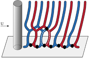
Figure 8. Flow past a cylinder with side wall: schematic of the (a) fork-type ( $D_f$) and (b) connected fork-type (
 $D_{fc}$) dislocations with ring-like structure highlighted in broken lines. The clockwise and anti-clockwise vortices are shown in blue and red colour, respectively. The filled circles indicate the connections between the vortices of opposite polarity.
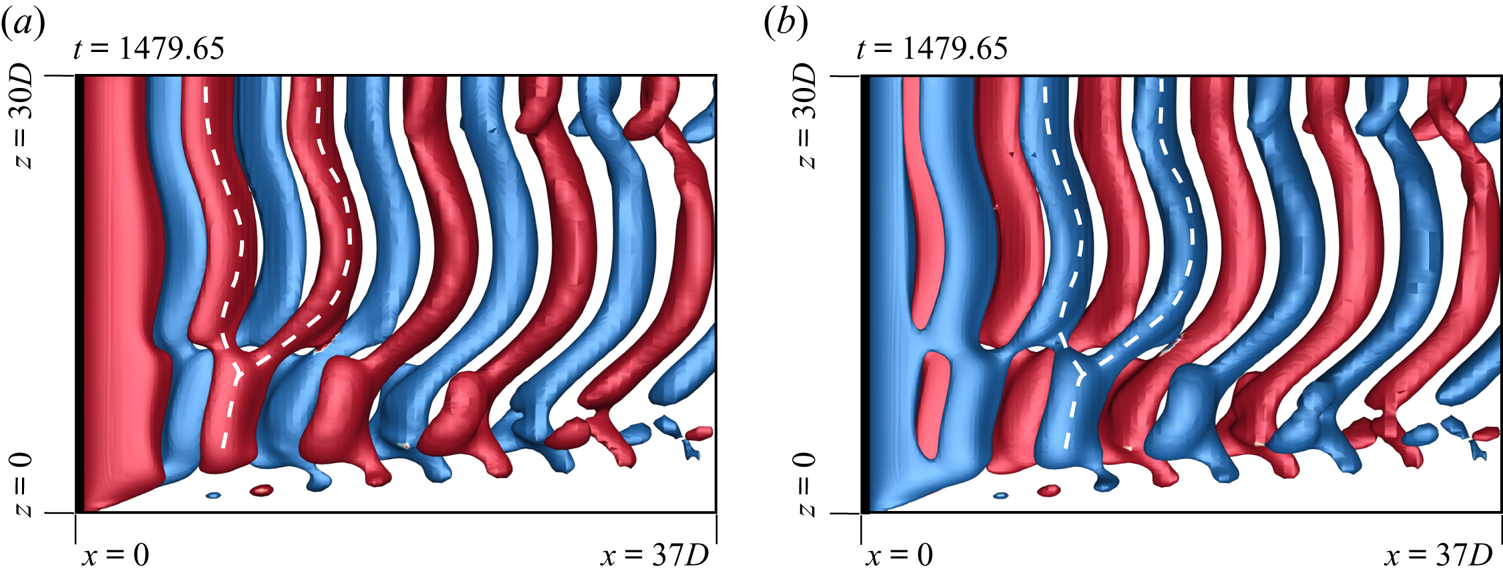
Figure 9. Flow past a cylinder with side wall:  $xz$-view of instantaneous
  $Q$ (
$Q$ ( ${=}0.001$) iso-surfaces coloured with spanwise component of vorticity (
 $\omega _z = \pm 0.01$) for
  $(AR, \textit {Re})=(60, 60)$ depicting the fork-like connection for (a) anti-clockwise rotating vortices and (b) clockwise rotating vortices at
  $t=1479.65$. In (a) the flow is visualized from a negative
  $y$ side, whereas it is seen from a positive
  $y$ side in (b).

Figure 10. Flow past a cylinder with side wall:  $xz$-view of instantaneous
  $Q$ (
$Q$ ( ${=}0.001$) iso-surface coloured with spanwise component of vorticity (
 $\omega _z = \pm 0.01$) for
  $(AR, \textit {Re})=(70, 90)$ depicting the connected fork-type dislocation at
  $t=823.7$. The enlarged view of the connection of vortices with opposite polarity at the cell boundary is shown alongside. The ring-like structure formed owing to the connection of vortices is highlighted.
Figure 11. Flow past a cylinder with side wall:  $xz$-view of instantaneous
  $Q$ (
$Q$ ( ${=}0.0005$) iso-surfaces coloured with spanwise component of vorticity (
 $\omega _z = \pm 0.01$) for
  $(AR, \textit {Re})=(60, 70)$ at (a)
  $t=1021.7$ and (b)
  $t=1039.2$ depicting mixed-type vortex dislocation. The transformation from fork-like structure to ring-like structure is highlighted as the dislocation convects downstream.
4.2.3. Oblique angle of vortices
Let  $\theta$ denote the oblique angle of the vortices in a cell, with the axis of the cylinder (table 2). Consistent with the findings of Behara & Mittal (Reference Behara and Mittal2010b), the present computations show that
  $\theta$ is constant in certain cases, whereas it varies along the span and with time for others. As listed in table 2, these two situations are represented by
  $\theta _{c/v}$, where the subscripts ‘
 $c$’ and ‘
 $v$’ indicate constant and varying oblique angle, respectively. In general, the second cell has the largest spanwise extent. Therefore, the classification with respect to
  $\theta$ is made on the basis of the second cell in case of multiple cells in the flow. In the case of single cell, the classification is based on
  $\theta$ in the end cell. Figures 4(c) and 4(d) show the flow for three- and four-cell cases at different time instants. The variation of the angle of shedding in the second cell is evident in both cases. This variation is further confirmed by the frequency spectra shown in figures 5(c) and 5(d). In addition to a dominant frequency, there are other frequencies as well that indicate that the shedding frequency is time varying. Williamson (Reference Williamson1988) proposed that the shedding frequency and oblique angle are related by the cosine rule. Behara & Mittal (Reference Behara and Mittal2010b) demonstrated that this relationship also holds when the oblique angle of the vortices varies along span and with time. Consistent with their observation, the present work shows that the shedding frequency varies with time when
  $\theta$ is not constant.
For the two-cell case, figure 4(b) reveals that the oblique angle in the second cell is constant with time and along span. For the single-cell case as well, shown in figure 4(a), the oblique angle of the end cell is invariant. Frequency spectra presented in figures 5(a) and 5(b) for both cases show a sharp peak which is consistent with the observation from the flow in figures 4(a) and 4(b) that the vortex shedding frequency and the oblique shedding angle are constant in these cases. Figure 6 shows the behaviour of  $\theta$ on the
  $AR$–
$AR$– $\textit {Re}$ plane. It can be concluded that a single cell is always associated with constant
  $\theta$. Three cells and higher exhibit varying
  $\theta$. The two-cell cases are most interesting.
  $\theta$ varies along span and with time for
  $\textit {Re}<60$. However, for larger
  $\textit {Re}$ (
 $\textit {Re}>60$),
  $\theta$ is constant for cylinders with span larger than a certain threshold (
 $AR\geqslant 50$) and varies for shorter span length (
 $AR<50$).
4.3. Time variation of shedding frequency and periodicity of vortex dislocations
To investigate the spatio-temporal variation of the vortex shedding frequency, we consider the time histories of the cross-flow component of velocity at various spanwise locations. The locations at which the velocity is sampled correspond to ( $x/D=5,\ y/D=0.25$) and are
  $2.5D$ apart along the span. The time period of each cycle, from the time histories, is utilized to estimate the instantaneous vortex shedding frequency. This non-dimensional frequency is referred to as
  $\widetilde {St}_{v}$. The spanwise and time variation of
  $\widetilde {St}_{v}$ is shown in figures 12(a) and 13(a) for
  $(AR, \textit {Re})=(60, 60)$ and
  $(60, 75)$, respectively. The former corresponds to the three-cell case whereas the latter is associated with two spanwise cells. The frequency spectra for the two cases are shown in figures 5(b) and 5(c), respectively. It can be observed from figure 12(a), for the three-cell case, that
  $\widetilde {St}_{v}$ shows significant temporal as well as spanwise variation in each cell. On the other hand figure 13(a), for the two-cell case, shows that
  $\widetilde {St}_{v}$ exhibits little variation within each cell.
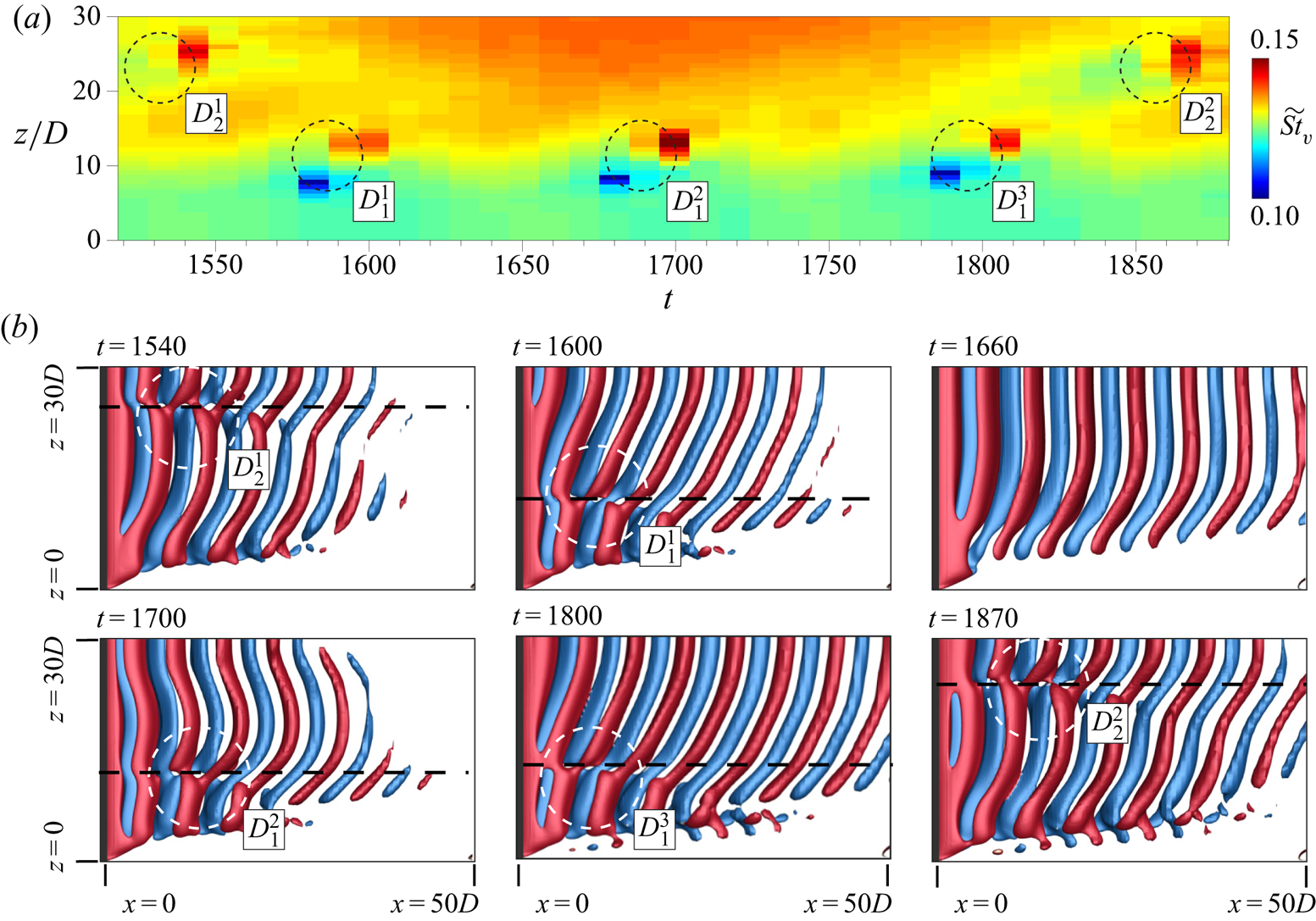
Figure 12. Flow past a cylinder with side wall. (a) Spatio-temporal variation of Strouhal number corresponding to the frequency of each cycle of cross-flow velocity component for  $(AR, \textit {Re})=(60, 60)$. The cross-flow velocity component data are obtained from spanwise separated probes placed
  $2.5D$ apart at (
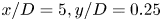 $x/D=5, y/D=0.25$). (b) The
  $Q$ (
$Q$ ( ${=}0.001$) iso-surfaces, coloured with spanwise component of vorticity (
 $\omega _z = \pm 0.1$), at various time instants. The cell boundaries as well as vortex dislocations are marked on the images.
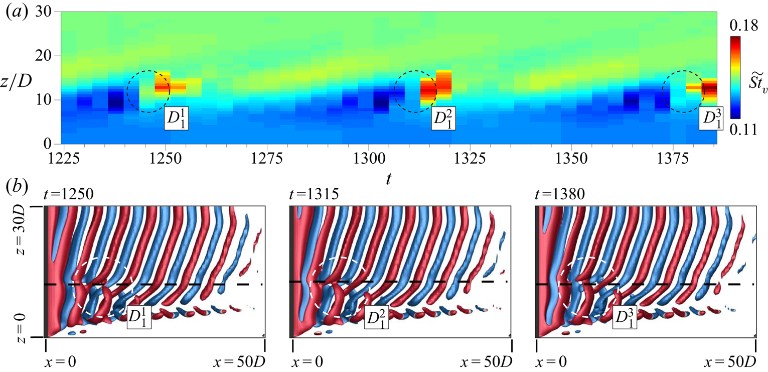
Figure 13. Flow past a cylinder with side wall. (a) Spatio-temporal variation of Strouhal number corresponding to the frequency of each cycle of cross-flow velocity component for 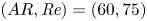 $(AR, \textit {Re})=(60, 75)$. The cross-flow velocity component data are obtained from spanwise separated probes placed
  $2.5D$ apart at (
 $x/D=5, y/D=0.25$). (b) The
  $Q$ (
$Q$ ( ${=}0.001$) iso-surfaces, coloured with spanwise component of vorticity (
 $\omega _z = \pm 0.1$), at various time instants. The cell boundaries as well as vortex dislocations are marked on the images.
Behara & Mittal (Reference Behara and Mittal2010b) observed that appearance of vortex dislocations coincides with local minima in  $\widetilde {St}_{v}$ followed by its sharp rise. Williamson (Reference Williamson1989) reported that the frequency of appearance of vortex dislocations corresponds to the beat frequency in the time signal near the junction of the cells. The present results are consistent with the observations of Behara & Mittal (Reference Behara and Mittal2010b) and Williamson (Reference Williamson1989). For the three-cell case in figure 12, the instantaneous frequency is found to attain a local minimum followed by a sharp rise at
  $t\sim 1600$, 1700 and 1800. A similar phenomenon occurs at
  $t\sim 1540$ and 1870, at a different spanwise location. Flow visualization at these time instants indeed display vortex dislocations
  $D_{1}$ and
  $D_{2}$ in the wake as seen in figure 12(b). The dislocation
  $D_{1}$ is found to appear every 100 time units, whereas
  $D_{2}$ appears around every 330 time units. The dislocation appearance frequency for
  $D_{1}$ and
  $D_{2}$, from these numbers, is estimated to be 0.0100 and 0.0030, respectively. The beat frequencies for
  $D_{1}$ and
  $D_{2}$, estimated from the time histories, are 0.0097 and 0.0031. The similarity between the beat frequency and that of the appearance of vortex dislocations is consistent with the findings of Williamson (Reference Williamson1989). Similarly, for the two-cell case presented in figure 13, the dislocation
  $D_{1}$ is found to appear at
  $t\sim 1250$, 1315 and 1380 marked as
  $D_{1}^{1}$,
  $D_{1}^{2}$ and
  $D_{1}^{3}$, respectively. The dislocation
  $D_{1}$ appears every 65 time units with an appearance frequency of 0.0154. The corresponding beat frequency is 0.0147. The low-frequency modulation in time histories of cross-flow velocity component observed in figure 5(b–d) can be attributed to vortex dislocations appearing in the wake. For the single-cell case shown in figure 4(a), the time histories in figure 5(a) do not show any modulation in line with the observation of Behara & Mittal (Reference Behara and Mittal2010b). Figure 13(a) shows a periodic oblique spanwise variation between the appearance of dislocations. This activity in the near wake is perhaps responsible for the generation of vorticity near the wall as seen in figure 13(b).
Figure 14 presents the variation of the frequency of appearance of vortex dislocations  $D_{1}$ and
  $D_{2}$ with
  $\textit {Re}$ for certain two- and three-cell cases. Both
  $D_{1}$ and
  $D_{2}$, appear more frequently with increase in
  $\textit {Re}$. However, the rate of increase in the frequency decreases with increase in
  $\textit {Re}$. This is consistent with the finding of Behara & Mittal (Reference Behara and Mittal2010b). In the case of three cells, the dislocation
  $D_{1}$ appears more frequently as compared with
  $D_{2}$. Combining this with the observations made from the four-cell case (not shown here), it is noted that the dislocation appearance frequency is maximum close to the side wall and decreases towards the centre of the cylinder.

Figure 14. Flow past a cylinder with side wall: variation of the frequency of appearance of vortex dislocations (a)  $D_{1}$ and (b)
  $D_{2}$ with
  $\textit {Re}$.
4.4. Global linear stability analysis
Figure 3 shows the variation of cellular structure of the flow in the  $AR$–
$AR$– $\textit {Re}$ plane. To explore the cause of the formation of cells, and the associated rich flow structure, a global linear stability analysis was conducted. First, a biglobal linear stability analysis was carried out for the
  $Re=100$, steady and two-dimensional flow to assess the spanwise structure of the flow in the absence of end walls. The most unstable eigenmode corresponding to perturbations with certain spanwise periodicity were computed. They are found to be the oblique modes of vortex shedding. None of the modes displayed any cellular structure, thereby implying the vital role of end conditions. The modes from the linear stability analysis were used as initial condition for direct time integration of the flow equations, with slip condition on the velocity at the lateral boundaries, to study the evolution of the flow including that in the nonlinear regime. The computations bring out the significance of the nonlinear terms in predicting the correct convection speed of the vortices, their frequency of shedding and their oblique angle to the axis of the cylinder.
Next, triglobal linear stability analysis was carried out for the  $AR=60$ steady flow with a side wall, for various
  $Re$. For all the cases, the most unstable mode is associated with single cell and the vortices are almost parallel to the axis of the cylinder. The higher modes exhibit cellular structure. However, as is assumed in a global linear stability analysis, the vortex shedding frequency is uniform along the span. The details of this analysis are presented in Appendix B. We surmise that the nonlinear terms play a significant role in the evolution of the various attributes of the flow.
4.5. Evolution of the flow
A direct numerical simulation is initiated with the steady flow for the case of  $(AR, \textit {Re})=(60, 70)$ to explore the time evolution of the flow. No explicit disturbance is imposed on the flow. Nevertheless, the numerical and round-off errors in the computations act as perturbations to the steady flow. These perturbations are expected to excite several modes. However, the eigenmode with the largest growth rate is expected to dominate the others. The time histories of drag and lift coefficients from the simulation are shown in figure 15. The enlarged views during the initial time are also shown. As the disturbances are very small at initial time, their growth is governed by the linearized equations. As the disturbance becomes larger, nonlinear effects gain prominence. The divergence of the mean drag coefficient from the value for the steady flow is an indication of the departure of the flow from linearity. The nonlinearity also causes the amplitude of the lift coefficient to depart from an exponential growth and approach a saturated value. It is seen from the figure that nonlinear effects become significant beyond
  $t\sim 250$.

Figure 15. Flow past a cylinder with side wall: time histories of the force coefficients obtained from direct numerical simulation initiated with the steady flow for  $(AR, \textit {Re})=(60, 70)$. Corresponding enlarged views during the initial time are shown in the bottom row.
Figure 16 shows the instantaneous flow at various time instants. The vortices are nearly parallel to the axis of the cylinder at  $t=200$ and 250, and form a single cell. This is consistent with the linear stability analysis which predicts that the single-cell parallel shedding constitutes the most unstable eigenmode. The disturbance field, with respect to the steady flow, can be compared with the eigenmodes from the linear stability analysis. The flow is very similar to mode 1 shown in Appendix B (figure 24c). With the nonlinear effects assuming significance beyond
  $t=250$, the vortices begin to tilt near the side wall, whereas they continue to be parallel to the axis of the cylinder towards mid span. This can be observed from figure 16 for the flow at
  $t=280$. The observation is consistent with that by Williamson (Reference Williamson1989) that the oblique front starts at the ends and propagates inwards. This is further confirmed by the flow at
  $t=310$. The evolution of the cellular structure in the flow can be seen in figure 16. Linkages develop between the ends of the adjacent pair of rotating and counter-rotating vortices at
  $t=310$. In contrast, the vortices diffuse near the end wall as seen from the frames corresponding to earlier time. Williamson (Reference Williamson1989) proposed that the oblique vortex shedding becomes unstable and leads to formation of cells when the oblique angle of the shed vortices reaches a certain critical value. Indeed, the flow at
  $t=340$ shows increased oblique angle of the vortices towards the mid-span and appearance of two spanwise cells separated by a fork-type vortex dislocation in the wake. The flow continues to evolve and reaches a saturated state at
  $t\sim 700$ as indicated by the time histories of the force coefficients (figure 15). The fully developed unsteady flow is associated with vortex dislocations of the mixed type. As seen from figure 16, the dislocation is of the fork type at
  $t=840$. It transforms to the ring type as it convects downstream as seen in the frame corresponding to
  $t=860$. In addition, the oblique angle of the vortices, for the fully developed unsteady flow, is constant along the span and invariant with time. This is seen in the pictures at
  $t=840$, 860 and 900. The fully developed flow exhibits all the attributes as per the description in figure 6.
Figure 16. Flow past a cylinder with side wall:  $xz$-view of
  $Q$ (
$Q$ ( ${=}0.0005$) iso-surfaces coloured with spanwise component of vorticity (
 $\omega _z = \pm 0.01$) at different time instants for
  $(AR, \textit {Re})=(60, 70)$. Also marked in (g,h) is the fork-type dislocation and ring-like structure.
A direct numerical simulation initiated with the mode 1, from the triglobal linear stability analysis, superposed with the steady base flow, was also carried out for this case. The evolution of the flow (not shown here) is very similar to that of the case described previously, except that it occurs at an accelerated pace. The flow reaches a saturated state much sooner. These simulations bring out the very significant role of the nonlinearities on the evolution of the flow. Even though the single cell with close to parallel vortices is the most unstable mode in the linear regime, the nonlinear effects that kick in after the disturbances become sufficiently large following an exponential-in-time linear growth, lead to a two-cell structure with oblique vortices.
4.6.  $\textit {Re}=90$ flow for low $AR$


Figure 3 shows that the end conditions stabilize the flow even at relatively large  $\textit {Re}$. We consider the
  $\textit {Re}=90$ flow for various
  $AR$. Triglobal linear stability analysis of the steady flow is carried out to assess its stability. The residual of the eigenmodes obtained for various
  $AR$ at
  $Re = 90$ is approximately
  $1 \times 10^{-9}$. The variation of the growth rate of the most dominant mode with
  $AR$ is shown in figure 17(a). The critical
  $AR$ beyond which the steady flow loses stability is
  $AR=7.67$. These findings are consistent with the results from direct numerical simulations and marked in figure 3. Specifically, the flow for
  $AR=7$ is found to be steady whereas the
  $AR=9$ case becomes unsteady. Also shown in figure 17(a) is the spanwise component of the vorticity field for the real part of the most unstable eigenmode for
  $AR=5$ and
  $9$. To explore the effect of end wall on the time evolution of the flow, we carry out direct numerical simulations for
  $AR=7$ and
  $9$ initiated with the fully developed two-dimensional unsteady flow. The time histories of the lift coefficient are shown in figure 17(b) and the spanwise vorticity at the
  $x$–
$x$– $z$ plane passing through the axis of the cylinder is shown at various time instants for the two flow in figure 18. Although the flow for
  $AR=7$ achieves a steady state, the
  $AR=9$ case leads to limit cycle oscillations with oblique vortex shedding in a single cell across the span of the cylinder.
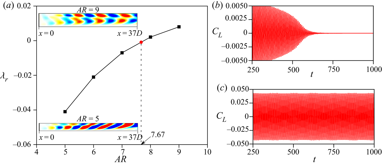
Figure 17. Flow past a cylinder with side wall at  $\textit {Re} = 90$. (a) Variation of growth rate of the dominant mode with
  $AR$. The spanwise vorticity field in the
  $x$–
$x$– $z$ plane for the real part of the eigenmode corresponding to the eigenvalue with largest real part is shown in the inset for two values of
  $AR$. (b,c) Time histories of lift coefficient for the direct numerical simulations initiated with unsteady two-dimensional flow for (b)
  $AR = 7$ and (c)
  $AR = 9$.

Figure 18. Flow past a cylinder with side wall at  $\textit {Re} = 90$: spanwise vorticity field in the
  $x$–
$x$– $z$ plane at various time instants for (a–d)
  $(AR, \textit {Re})= (7, 90)$ and (e–h)
  $(AR, \textit {Re})=(9, 90)$.
4.7. Simulation of full span, initiated from half-span
To assess the validity of the assumption of symmetry of the flow about mid-span of the cylinder, we carried out a few simulations for the full span. The flow solution from the simulations for half the span is reflected about mid-span and used as initial condition. The test cases chosen for the full-span simulations include combinations of ( $AR, Re$) that yield two, three and four cells across half the span of cylinder. These cases are highlighted in figure 6 via solid symbols. Of all the cases, only those that lie in the hatched region shown in figure 6 develop asymmetry about the mid-span; the others retain their symmetry. Three of the several cases, that were tested, are shown in figure 19. Figure 19(a) shows the vortex structure for
  $(AR, \textit {Re}) = (90, 54)$, the case with two cells in half the span, at three time instants. The variation of the dominant frequency in the power spectra of the time histories at various span locations in the wake is also shown in the figure. It is observed that despite the asymmetry about mid-span, the flow retains the two-cell structure along half-span and the associated dislocations. The flow also retains all other attributes, listed in table 2, of the flow that are seen in the simulations with imposed symmetry along mid-span. Shown in figures 19(b) and 19(c) are the results for
  $(AR, \textit {Re}) = (80, 54)$ and (
 $80, 55$), respectively. Both these cases correspond to the four-cell structure in half-span. While the flow retains symmetry about mid-span for the former, the latter develops asymmetry. In all cases, the cell structure as well as other attributes of the flow are retained.
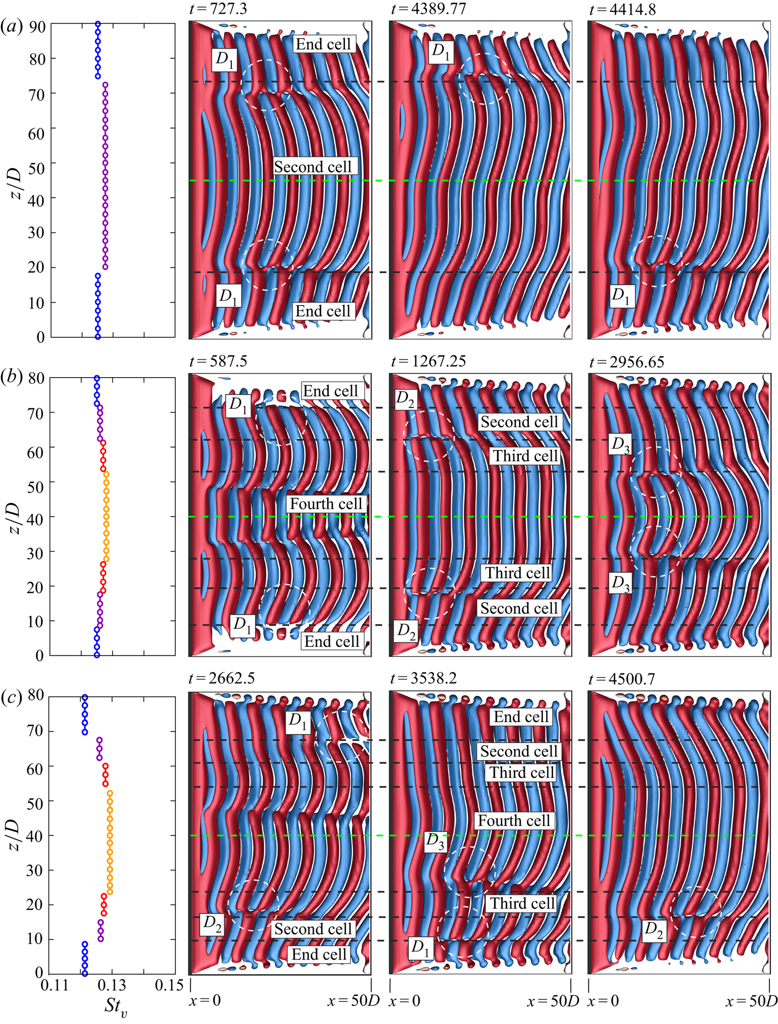
Figure 19. Full span simulation of flow past a cylinder with side wall:  $Q$ (
$Q$ ( ${=}0.0002$) iso-surface coloured with spanwise component of vorticity (
 $\omega _z = \pm 0.01$) for (a)
  $(AR, \textit {Re})=(90, 54)$, (b)
  $(AR, \textit {Re})=(80, 54)$ and (c)
  $(AR, \textit {Re})=(80, 55)$. The dislocations as well as the boundaries of the cells are marked in broken white and black lines, respectively. The broken green line is along the mid-span of the cylinder.
5. Conclusions
The cellular nature of vortex shedding for flow past a cylinder with side wall has been investigated numerically utilizing a stabilized finite element method. The no-slip condition imposed on the side wall promotes the boundary layer formation. The length of the side wall is kept such that the boundary layer thickness, as the flow approaches the cylinder, is constant for all computations carried out. In this scenario it is expected that the state of the flow is determined by ( $AR, \textit {Re}$). The computations have been carried out for cylinders of varied
  $AR$ ranging from 5 to 90 and flows at
  $\textit {Re}$ varying between 50 and 95. Symmetry conditions imposed at mid-span enable simulation of only one half the span length. To assess the validity of this assumption, computations for a few cases are carried out for the full span with no imposed condition of symmetry at mid-span. For these simulations, the solution from half the span is reflected along the mid-span to generate the flow for the entire span. It is found that in most cases the symmetry of the flow about the mid-span is retained. The flow loses symmetry for some of the cases corresponding to two and four cells in half the span. However, even in these cases the flow retains the attributes predicted by half-span simulations such as the number of cells, structure of dislocations and end vortices near the side wall. It would be interesting to explore, in future work, the full-span simulations for more cases and with different initial conditions. The computations bring out the various changes that the wake undergoes depending on the combination of (
 $AR, \textit {Re}$).
Experiments by Williamson (Reference Williamson1989) for cylinders with  $AR$ between
  $90$ and
  $240$ reveal that the wake has a three-cell structure for
  $\textit {Re}<64$, while only two cells exist along the span for
  $\textit {Re} >64$. A Strouhal discontinuity observed at
  $\textit {Re} = 64$ was also attributed to this change in oblique shedding mode. Compared to the experiments by Williamson (Reference Williamson1989), the computations in the present work are for lower
  $AR$ (between
  $5$ and
  $90$). It is interesting to compare the observations from the two studies for
  $AR=90$ which has been attempted in both the studies. The results from the present are broadly in agreement with the experimental observations, but also reveal more richness in the flow. Consistent with the study by Williamson (Reference Williamson1989), the present computations, for
  $AR=90$, show a transition from the three- to two-cell oblique shedding, albeit at a slightly lower
  $Re$ (
 ${\sim }61$). The slight change in the critical
  $\textit {Re}$ for the transition can be attributed to the difference in the end conditions for the two set-ups. The experiments by Williamson (Reference Williamson1989) used end plates of diameter between
  $10D$ and
  $30D$, whereas the present computations utilize a no-slip condition on the end wall. These would lead to different thickness of the boundary layer on the end wall/end plates as it approaches the cylinder. It was shown by Behara & Mittal (Reference Behara and Mittal2010b) that the boundary layer thickness at the end wall affects the oblique angle of vortices. Therefore, it is quite possible that the critical
  $\textit {Re}$ for the transition is affected as well.
The present computations reveal additional attributes of the flow. Some of these are highlighted in figures 3 and 6. For example, for the cylinder with  $AR=90$, the flow transitions from a one-cell to two-cell wake at
  $\textit {Re} \sim 50$ and than to a four-cell structure at
  $\textit {Re} \sim 55$. It reverts back to three cells along the span and subsequently to a two-cell wake with further increase in
  $\textit {Re}$. The structure of the dislocation, in the two-cell wake, undergoes a transition at
  $\textit {Re} \sim 70$ (see figure 6). It is conceivable that for larger
  $AR$ (
 $AR > 90$) the wake may be associated with even larger number of cells in certain range of
  $Re$. This could be of interest for a future study. Interestingly, the complexity of the transitions decreases with decrease in
  $AR$. For example, the flow is associated with a single-cell wake for
  $AR=20$, whereas it is steady for
  $AR=5$ for all the
  $Re$ considered. Barring the end vortex structure, that undergoes a transition from diffused to linked vortex structure at
  $\textit {Re} \sim 60$, the wake structure for
  $AR=20$ is similar at all
  $Re$. The critical
  $\textit {Re}$ for the onset of vortex shedding is found to decrease with increasing
  $AR$.
$AR$.
The structure of wake is significantly affected by  $AR$ and
  $\textit {Re}$. One way of understanding this from figures 3 and 6 is to observe the effect of varying
  $AR$ while holding
  $\textit {Re}$ constant. At each
  $\textit {Re}$ we identify two critical
  $AR$. The flow is steady for
  $AR < AR_{{cr}_{1}}$, whereas shedding with a single cell along the span is observed for
  $AR_{{cr}_{1}} < AR < AR_{{cr}_{2}}$. Two or more cells are observed for
  $AR > AR_{{cr}_{2}}$. In addition to the number of cells along span, the other attributes of the flow that vary with
  $AR$ and
  $\textit {Re}$ are the vortex dislocations between cells, oblique angle of the vortices and their structure close to the end wall. A broad classification of the flow in the
  $AR$–
$AR$– $\textit {Re}$ plane, based on these attributes, is summarized in figure 6. The oblique angle of vortices, in single-cell shedding, is constant along span. For two cells or more, it is found that, in general, the oblique angle of vortices varies along the span for
  $\textit {Re} \leqslant 60$ irrespective of
  $AR$. However, for larger
  $\textit {Re}$ the angle along the span is constant for
  $AR > 50$, approximately. The vortices diffuse out near the end wall for
  $\textit {Re} \leqslant 58$. They form linkages with neighboring vortices of opposite polarity for larger
  $\textit {Re}$. The type of dislocations across cells is found to correlate well with the structure of end vortices. Fork-type vortex dislocations and diffused end vortices are seen in the wake at low
  $\textit {Re}$. Connected fork-type dislocations occur at relatively large
  $\textit {Re}$.
The number of dislocations is one less than the number of cells along the span. They appear at the beat frequency, which is related to the difference in the frequency of shedding across the dislocation. In general, for three cells or more, these dislocations are not in phase. A spatio-temporal analysis of the frequency of the cross-flow component of velocity in the near wake shows that the appearance of dislocation coincides with a local minimum in the shedding frequency followed by a sharp rise. The dislocations close to side wall appear more frequently than those towards the mid-span. In addition, the frequency of dislocations increases with an increase in  $\textit {Re}$.
Global linear stability analysis was conducted to explore the reason for the formation of cells. Linear stability analysis for cylinders with infinite span reveals oblique shedding with constant angle along the span. The parallel shedding is found to be that with largest growth rate. The growth rate decreases with increase in oblique angle. No cell-like structures are observed in any of the linearly unstable modes. Further, it is found that the modes from the linear analysis do not follow the cosine rule relating the oblique angle of the vortices and their shedding frequency (Williamson Reference Williamson1988). The convection speed of the vortices is also grossly underpredicted by the linear analysis. Direct numerical simulations, with periodic boundary conditions at end walls, initiated with the linear modes bring out the significance of the nonlinearity on the flow. The flow structures evolve to satisfy the cosine rule as well as the correct speed of convection of vortices that is independent of the shedding angle (Williamson Reference Williamson1988). However, the flow is still devoid of cells, confirming the role of an end wall in cellular shedding.
Linear stability analysis of the steady flow past cylinder with an end wall was conducted for a variety of  $\textit {Re}$. In all cases, the mode with vortices parallel to the cylinder was found to be most unstable. The modes associated with cells have lower growth rate. These cells are, however, different than those seen in experiments and in direct numerical simulations. We recall, the disturbance in the global linear stability analysis assumes the same temporal frequency throughout the entire spatial domain. Therefore, the vortex shedding frequency across the cells is also same in each of the eigenmodes from global linear stability analysis. What, then, is the role of these eigenmodes in the cellular shedding? A direct numerical simulation initiated with the steady flow was carried out. As predicted by linear stability analysis, the unsteadiness in the flow develops via the parallel mode of shedding with no cells along the span. However, as the disturbance field evolves and the nonlinear terms gain significance an oblique front develops at the end wall and moves inward towards the mid span with time. This is followed by formation of cells along the span that are separated by vortex dislocations. These simulations bring out the significance of the nonlinear effects, especially in the presence of an end wall. For the flow with periodic boundary conditions along the span, the linear and nonlinear flows are qualitatively similar. However, in the presence of an end wall the two flows are qualitatively different in terms of cellular structure, vortex dislocations and end vortex structure.
This study brings out the complexity in the wake of a circular cylinder owing to the end conditions. It is expected that more complex geometries, including changes along the span, may further add to the complexities in the flow. It will be interesting to extend this work in future to higher  $\textit {Re}$ and to other geometries of practical interest.
Acknowledgements
The authors acknowledge the use of High Performance Computational (HPC) facility at Indian Institute of Technology Kanpur (IITK), established with the assistance of Department of Science and Technology (DST), India, and National PARAM Supercomputing Facility (NPSF) at Centre of Development of Advanced Computing (C-DAC), Pune, India. The help from Mr A. Verma, A. Lohia and S. Shobhit in computation of some of preliminary results and the lively discussions is gratefully acknowledged.
Declaration of interests
The authors report no conflict of interest.
Appendix A. Vortex identification
We briefly review and compare three methods for identifying vortex cores: the  $Q$,
$Q$,  $\lambda _2$ and
  $\varOmega$ criterion proposed by Hunt et al. (Reference Hunt, Wray and Moin1988), Jeong & Hussain (Reference Jeong and Hussain1995) and Liu et al. (Reference Liu, Wang, Yang and Duan2016), respectively. The velocity gradient tensor is decomposed as
  $\boldsymbol {\nabla } \boldsymbol {u}=\boldsymbol {\omega } + \boldsymbol{\mathsf{S}}$, where
  $\boldsymbol {\omega }= [\boldsymbol {\nabla } \boldsymbol {u} - (\boldsymbol {\nabla } \boldsymbol {u})^\textrm {T}]/{2}$ and
  $\boldsymbol{\mathsf{S}}= [\boldsymbol {\nabla } \boldsymbol {u} + (\boldsymbol {\nabla } \boldsymbol {u})^\textrm {T}]/{2}$ are, respectively, skew-symmetric and symmetric. We further define two scalars:
  $Q= [\omega_{ij}\omega_{ij}-{\mathsf{S}}_{ij}{\mathsf{S}}_{ij}]/{2}$ and
  $\varOmega ={\omega_{ij}\omega_{ij}}/({{\mathsf{S}}_{ij}{\mathsf{S}}_{ij}+\omega_{ij}\omega_{ij}})$. According to the
  $Q$ criterion, an eddy is identified by a positive value of
  $Q$. Let
  $\lambda _1$,
  $\lambda _2$ and
  $\lambda _3$ be the eigenvalues of the symmetric matrix
  $\boldsymbol {\omega }^2 + \boldsymbol{\mathsf{S}}^2$ such that
  $\lambda _1$ is the largest and
  $\lambda _3$ the smallest eigenvalue. In the
  $\lambda _2$ method, negative values of
  $\lambda _2$ are utilized to identify the minimum pressure in a plane normal to the axis of the vortex. As per the
  $\varOmega$ method, a value of
  $\varOmega \geqslant 0.5$, that represents the ratio of vorticity to the rate of deformation, is used to identify vortices in the flow.
The vortex structures identified by the three criteria for the flow corresponding to different combinations of ( $AR, Re$) are presented in figure 20. The top row in the figure is for the case of
  $(AR, Re)=(60, 70)$ associated with single cell and diffused end vortices. All three vortex identification criteria yield same flow structures. Similar is the observation for
  $(AR, Re)=(60, 75)$ shown in second row of the figure with two cells along half the span and linked end vortices. The
  $(AR, Re)= (60,70)$ flow is associated with a mixed-type dislocation, i.e. a fork-type dislocation convects downstream and forms a ring-like structure at a later time instant. Figure 21 shows the flow visualized with the three criteria at a time instant where the ring-like structure exists in the flow. Again, the vortex structures identified by the three methods are in excellent agreement.
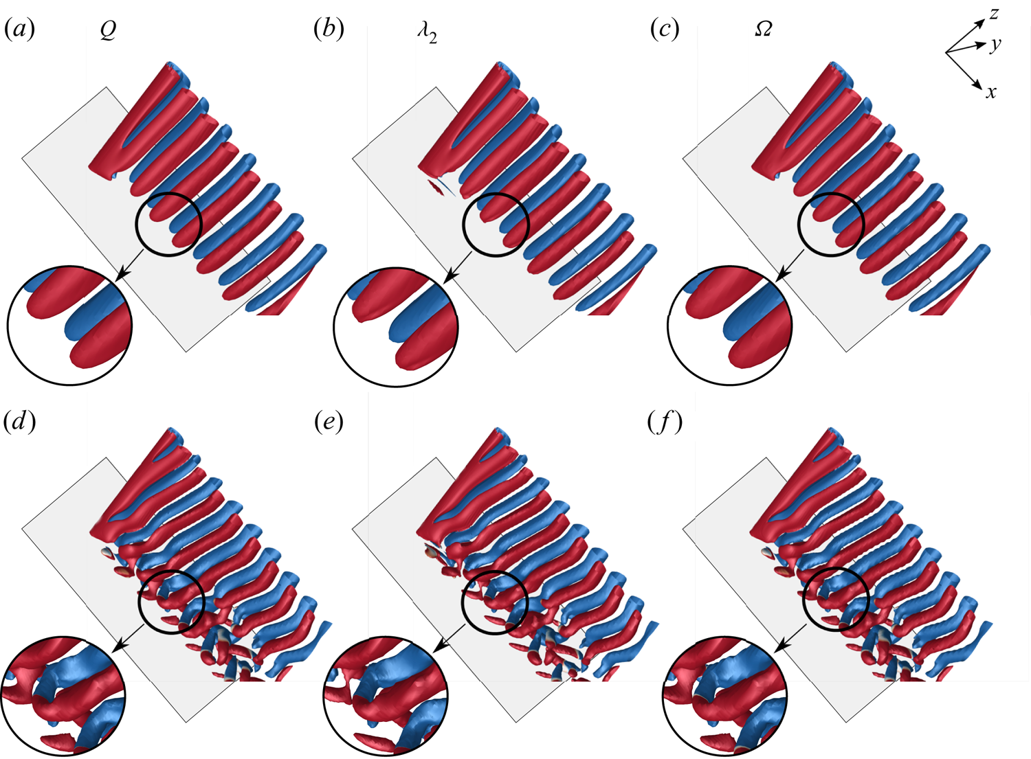
Figure 20. Flow past a cylinder with side wall: instantaneous flow structure visualized using  $Q = 0.0005$ (a,d),
  $\lambda _2 = -0.0005$ (b,e) and
  $\varOmega = 0.5$ (c, f) for
  $(AR, Re)=$(a–c) (
 $60, 50$) and (d–f) (
 $60, 75$). The iso-surfaces are coloured with spanwise component of vorticity (
 $\omega _z = \pm 0.01$). The side wall is shown for reference.

Figure 21. Visualization of the  $(AR, Re) = (60, 70)$ flow past a cylinder with side wall with different criterion for identification of vortices: iso-surfaces of (a)
  $Q = 0.0005$, (b)
  $\lambda _2 = -0.0005$ and (c)
  $\varOmega = 0.5$ coloured with spanwise component of vorticity (
 $\omega _z = \pm 0.01$). The ring-like structure formed after the convection of fork-type dislocation is highlighted in each image.
Appendix B. Linear stability analysis of steady flow
B.1. Biglobal linear stability analysis of two-dimensional steady flow
First, linear stability analysis is carried out for the two-dimensional steady flow past a cylinder of infinite span for perturbations that are periodic along the span with wavenumber  $\beta$ (see (2.6)). For each
  $\beta$, we seek the rightmost eigenvalue,
  $\lambda =\lambda _{r} + \textrm {i} \lambda _{i}$. A positive
  $\lambda _r$ indicates an unstable mode.
  $\lambda _i$ is related to the time-frequency of the instability. Table 3 lists the characteristic details of the eigenmodes with largest growth rates obtained from the biglobal linear stability analysis at
  $\textit {Re}=100$ for different
  $\beta$. The residual, per degree of freedom, is smaller than
  $1 \times 10^{-8}$ for each case. The spanwise vorticity for the eigenmodes corresponding to the rightmost eigenvalue for certain
  $\beta$ are shown in figure 22(a). Here
  $\beta =0$ corresponds to parallel shedding, whereas non-zero
  $\beta$ results in oblique shedding. Also marked on the figure is the oblique angle (
 $\theta _{LSA}$) of the vortices and the spacing (
 $d$) between the adjacent vortices of similar polarity. Table 3 indicates that
  $\beta =0$, i.e. parallel shedding, has the highest growth rate and that
  $\lambda _{r}$ decreases with increase in
  $\beta$. These computations confirm that the parallel and oblique shedding are intrinsic to the flow past a cylinder and that, boundary conditions permitting, the parallel mode is the preferred mode of vortex shedding. The Strouhal number for each
  $\beta$ (
 ${=}St_{\beta }$), calculated from
  $\lambda _{i}$, is also listed in the table along with
  $\theta _{LSA}$. We note that
  $\theta _{LSA}$ increases and
  $St_{\beta }$ decreases with increase in
  $\beta$.
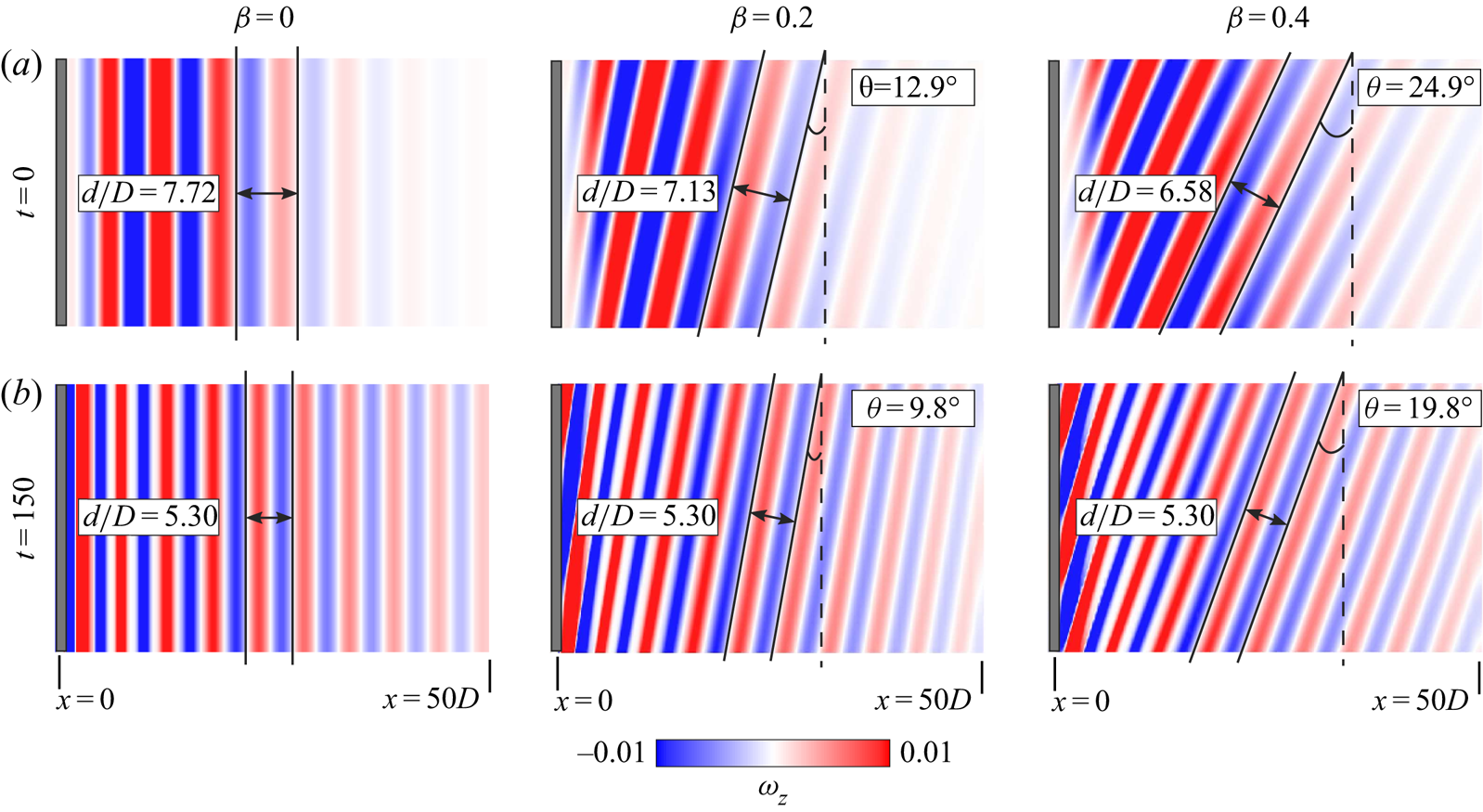
Figure 22. Direct numerical simulation initiated with the eigenmodes corresponding to  $\beta =0.0$, 0.2 and 0.4 superposed on the steady base flow at
  $\textit {Re}=100$: spanwise component of vorticity of the perturbation field at (a)
  $t=0$ and (b)
  $t=150$.
Table 3. Global linear stability analysis of two-dimensional steady flow past a cylinder with three-dimensional spanwise periodic perturbations at  $\textit {Re}=100$: characteristic details of the eigenmodes with largest growth rate for different values of
  $\beta$. Here
  $\lambda _{r}$ and
  $St_{\beta }$ are the growth rate and shedding frequency,
  $\theta _{LSA}$ is the measured angle of inclination of the vortices,
  $\theta _{St}$ is obtained from the cosine rule,
  $\theta _{St} = \cos ^{-1}St_{\beta }/St_{\beta =0}$, and
  $U_{c}$ is the convection speed of vortices that is obtained from the direct numerical simulation, in the linear regime, and initiated with the corresponding eigenmode.
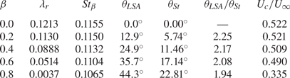
Williamson (Reference Williamson1988) proposed that the frequencies for the parallel and oblique vortex shedding are related via a cosine rule:  $\cos \theta = St_{\theta }/St_{||}$. Here,
  $\theta$ is the angle of the oblique vortices whereas
  $St_{\theta }$ and
  $St_{||}$ are the Strouhal numbers for the oblique and parallel shedding, respectively. Listed in table 3 is the
  $\theta _{St}$ estimated from the
  $St_{\beta }$ obtained from linear stability analysis. The expression used is
  $\theta _{St}=\cos ^{-1} {St_{\beta }/St_{\beta =0}}$. It is noted that the
  $\theta _{St}$ so estimated does not match
  $\theta _{LSA}$, which is the geometric oblique angle of the vortices as shown by the eigenmode (figure 22a). In fact, for low
  $\beta$,
  $\theta _{LSA}$ is more than twice the value of
  $\theta _{St}$. This suggests that the cosine rule, as proposed by Williamson (Reference Williamson1988) from experiments with end control plates, is not valid in the linear regime.
It is also clear from table 3 and figure 22(a) that the linear stability analysis of the two-dimensional flow does not explain the cellular shedding observed in the flow past a cylinder. It appears that the presence of an end wall is vital to the cellular structure. In addition, the analysis shows that the eigenmodes from the linear stability analysis do not respect the cosine rule. It is well known that the nonlinear effects play a major role in the realization of the fully developed unsteady flow. To explore the effect of nonlinearity on the oblique shedding and cellular structures, direct numerical simulation of the flow is carried out wherein the initial condition of the flow is the steady flow superposed with the eigenmode from the linear stability analysis. Periodic flow conditions are applied at the side walls. The span-length of the cylinder is chosen to accommodate an integer number of span-wise wavelengths ( $\lambda _{z}=2 {\rm \pi} /\beta$) of the instability. The direct numerical simulation is expected to yield the time evolution of the disturbance in the form of the most unstable eigenmode for each
  $\beta$. Computations are carried out until the flow achieves a limit cycle. Figure 22(b) shows the instantaneous perturbation field for the fully developed unsteady flow for
  $\beta =0$, 0.2 and 0.4. The vortices for
  $\beta =0$ continue to remain parallel to the axis of the cylinder, whereas the vortices for the other
  $\beta$ remain inclined, albeit at a reduced angle. The angle of the vortices is marked in the figure. The spacing between the vortices also undergoes a reduction, as compared with that in the initial condition. In fact, as hypothesized by Williamson (Reference Williamson1989) and confirmed by his experimental measurements, the spacing between the vortices, for the fully developed unsteady flow, is independent of the oblique angle. This is not the case for the eigenmodes of the linear stability analysis.
Another interesting parameter that is related to the frequency of vortex shedding and the spacing between the vortices is the convection speed of the vortices. Williamson (Reference Williamson1989) found that the vortices convect at about 90 $\%$ the free-stream speed. The streamwise convection speed (
 $U_{c}$) of the vortices is estimated from direct numerical simulation. Table 3 lists the speeds estimated during the initial stages of the direct numerical simulation, initiated from the eigenmodes of linear stability analysis. At this stage, the disturbance is small, compared with the steady flow, and the nonlinear effects are insignificant. This
  $U_{c}$, therefore, is attributed to the convection speed of the vortices of the eigenmodes. Clearly, they vary with
  $\beta$ (and, therefore, with
  $\theta _{LSA}$) and are much lower than the speed reported by Williamson (Reference Williamson1989). Figure 23 shows the time evolution of the convection speed of vortices,
  $St$ and oblique angle of the vortices for the simulations corresponding to
  $\beta =0$, 0.2 and 0.4. The effect of nonlinearity on the flow is very significant. The convection speed of the vortices saturates to 0.88
 $U_{\infty }$, approximately, which is in very good agreement with the experimental observation of Williamson (Reference Williamson1989). In figure 23(b) for
  $\beta =0$, the
  $St$ remains constant for
  $t> 50$ with a value of
  $0.16$ and is in good agreement with the simulation of two-dimensional flow past circular cylinder (Sheard, Thompson & Hourigan Reference Sheard, Thompson and Hourigan2003). Here
  $St$ and
  $\theta$, for the fully developed unsteady flow, are also found to satisfy the cosine rule. This establishes the significance of nonlinear effects in the flow. It is also concluded that a side wall or end plate is necessary for formation of spanwise cells in the wake.

Figure 23. Direct numerical simulations initiated with the eigenmodes corresponding to  $\beta =0.0$, 0.2 and 0.4 superposed on the steady base flow at
  $\textit {Re}=100$: time evolution of (a) the normalized convection speed,
  $U_{c}/U_{\infty }$, (b) normalized shedding frequency,
  $St$, and (c) angle of oblique vortices,
  $\theta$. The
  $(x/D, y/D)$ for the location where
  $U_{c}$,
  $St$ and
  $\theta$ are estimated is
  $(5,1.4)$,
  $(10,1.4)$ and
  $(20,0)$, respectively. The spanwise location for all the estimates is
  $z=L_{z}/2$.
B.2. Triglobal linear stability analysis for finite cylinders with side wall
With reference to figure 3, computations are carried out for the cylinder with a span corresponding to  $AR=60$ for three values of
  $\textit {Re}$: 55, 60 and 70. The unsteady flows for
  $\textit {Re}=55$ and 60 are associated with three cells, whereas two cells are observed for the
  $\textit {Re}=70$ flow (see figure 3). First, for each
  $\textit {Re}$, the steady flow is computed for the problem set-up shown in figure 1, by dropping the unsteady terms from the flow equations. For the disturbance of the type described in (2.7), we track the first few eigenvalues that have the largest real part. They are listed in table 4 for the three
  $\textit {Re}$ considered. For each
  $\textit {Re}$, all the unstable modes as well as one stable mode are listed. All these modes are found to be complex. Therefore, they appear as conjugate pairs. The modes are numbered in the order of decreasing growth rate. Mode 1 is associated with the largest real part and is, therefore, the one with largest growth rate. The spanwise vorticity of the real part of the eigenmodes for the three
  $\textit {Re}$ is shown in figure 24.
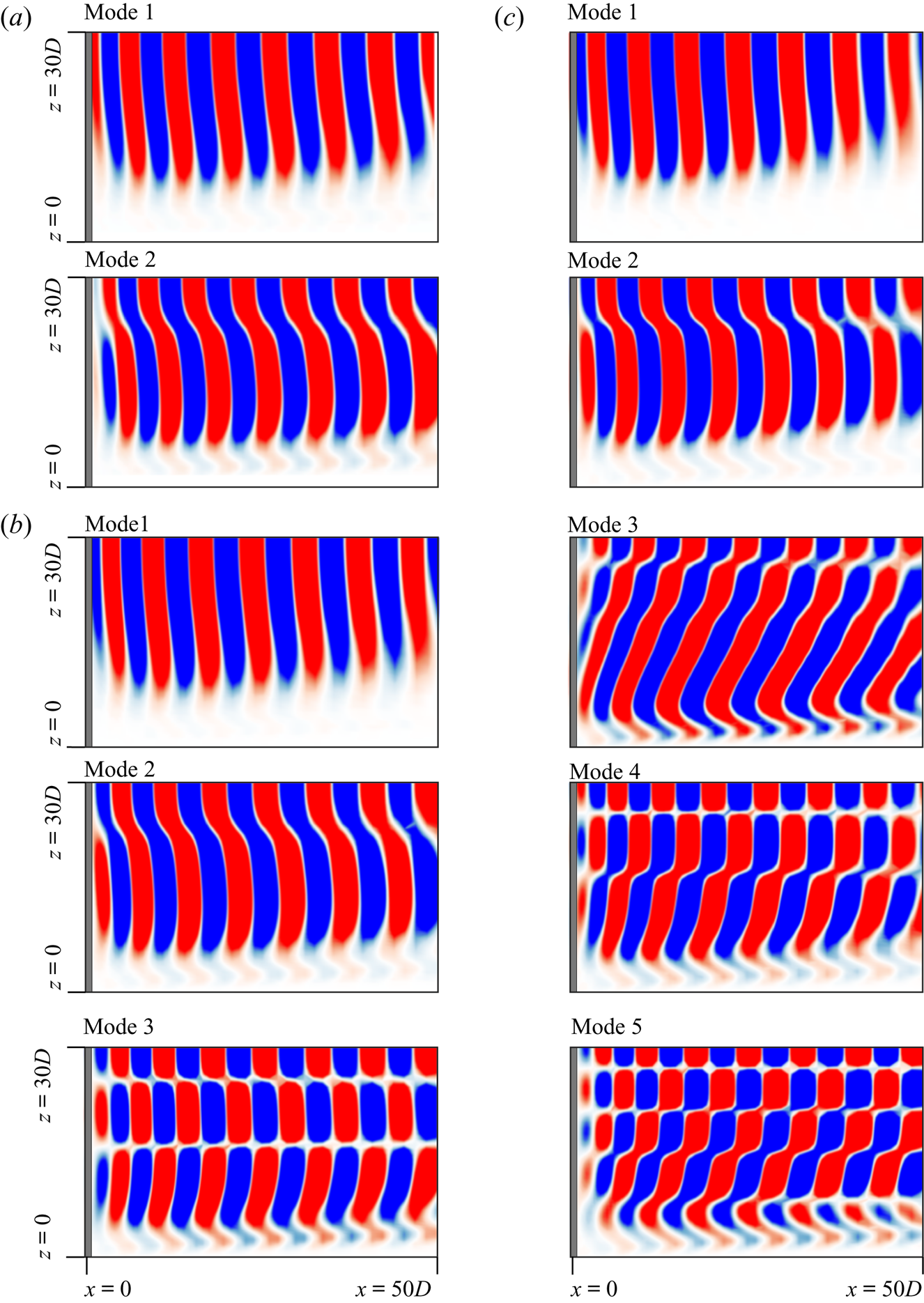
Figure 24. Global linear stability analysis of a finite cylinder with side wall: spanwise component of vorticity of the eigenmodes with largest growth rate and listed in table 4 for (a)  $(AR, \textit {Re})=(60, 55)$, (b)
  $(AR, \textit {Re})=(60, 60)$ and (c)
  $(AR, \textit {Re})=(60, 70)$.
Table 4. Global linear stability analysis of a finite cylinder of  $AR=60$ with side wall: details of the eigenmodes with largest growth rates for different values of
  $\textit {Re}$. Here
  $\lambda _{r}$ and
  $St$ are the growth rate and shedding frequency of the mode, respectively. The residual for each mode is presented in parentheses.
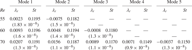
Mode 1, for all  $\textit {Re}$, has a single-cell structure and the vortices are almost parallel to the axis of the cylinder. Mode 2 exhibits a two-cell structure which becomes more apparent with increase in
  $\textit {Re}$. The vortices are still parallel to the axis of the cylinder except at the boundary of the two cells. Mode 3 has been tracked only for
  $\textit {Re}=60$ and 70. It shows a three-cell structure for
  $\textit {Re}=60$ with the vortices aligned parallel to the axis of the cylinder. Interestingly, the cellular structure is not due to the difference in the vortex shedding frequency across the cells, rather it is due to stagger of vortices of different polarity across the span. Mode 3 for the
  $\textit {Re}=70$ flow shows a two cell structure. It is different from the two-cell structure of mode 2 in the sense that vortex cores in cell 1 are oblique in mode 3. Modes 4 and 5 for the
  $\textit {Re}=70$ flow show three and five cells along the span, respectively.
At this point, we make a few observations regarding the global linear stability analysis. In the disturbance field, described by (2.6) and (2.7), the time frequency as well as growth rate are global in nature, that is, they do not vary spatially. In particular, this implies that the ‘vortex shedding’ frequency for the resulting eigenmodes is constant along the span. Cellular shedding, on the other hand, as seen from figure 4, is associated with a change in vortex shedding frequency across the cell boundary. Therefore, eigenmodes from the global linear stability analysis cannot be expected to replicate this behaviour of cellular shedding associated with a ‘nonlinear’ flow.