4.1 Mean velocity profiles

Mean velocity profiles are obtained for each case by averaging the streamwise velocity field in the wall-parallel plane at each wall-normal location. Figure 3 shows the inner-scaled, mean streamwise velocity, $U^{+}$ , for all cases, including that of the smooth-wall DNS at $Re_{\unicode[STIX]{x1D70F}}=400$ . The log law $U^{+}(y^{+})=(1/0.41)~\text{ln}(y^{+})+5.5$ is also included. While viscous stress is the only contributor to the drag in the smooth-wall case, figure 5 highlights the increased drag produced by roughness, including form-drag contributions to the overall wall shear stress. This increased drag modifies the mean velocity profile by an approximately constant downward shift in the log region of the flow, $\unicode[STIX]{x0394}U^{+}$ . This downward shift is observed for all rough-wall cases and can be determined by fitting the rough-wall mean velocity profiles with the log law as

(4.1) $$\begin{eqnarray}U^{+}(y^{+})=\frac{1}{\unicode[STIX]{x1D705}}\ln (y^{+})+5.5-\unicode[STIX]{x0394}U^{+}.\end{eqnarray}$$

The effective wall-normal origin, $d_{0}^{+}$ , is also determined by fitting the slope of the log law assuming $\unicode[STIX]{x1D705}=0.41$ . Table 2 summarizes these roughness-induced parameters for all cases. Finally, the equivalent sand-grain roughness height, $k_{s}^{+}$ , for each case can be determined by matching the $\unicode[STIX]{x0394}U^{+}$ observed to the sand-grain size that yields an equivalent $\unicode[STIX]{x0394}U^{+}$ from the measurements of Nikuradse (Reference Nikuradse1933). The main observation in figure 3 is the clustering of profiles based on the degree of packing of the surface roughness. The closely packed (hemispheres touching) case RH400-20-2 has a mean velocity that is intermediate to the smooth-wall cases and all other rough-wall cases. When the packing density of the roughness elements is high (i.e. low $d$ ), they effectively shelter one another and form narrow recirculation regions that isolate the outer flow from the roughness sublayer (Jiménez Reference Jiménez2004). Thus, the densely packed roughness in the RH400-20-2 cases is classified as the ‘d-type’ roughness whereas the cases RH400-20-3 and RH400-20-4 are commonly referred to as the ‘k-type’ roughness, based on the classification first introduced by Perry et al. (Reference Perry, Schofield and Joubert1969). Moreover, the mean velocity profiles for the rough-wall cases at $Re_{\unicode[STIX]{x1D70F}}=200$ (RH200-10-4) and $600$ (RH600-30-4) collapse very well in the log layer with RH400-20-4. This collapse is consistent with previous studies (Nikuradse Reference Nikuradse1933; Colebrook & White Reference Colebrook and White1937; Perry et al. Reference Perry, Schofield and Joubert1969, among others) wherein for ‘k-type’ roughness, the primary factor in determining $\unicode[STIX]{x0394}U^{+}$ is $k^{+}$ compared to other geometrical parameters. For ‘k-type’ roughness, $\unicode[STIX]{x0394}U^{+}$ can be related to $k_{s}^{+}$ via the study of Nikuradse (Reference Nikuradse1933) through the fully rough asymptote given by

(4.2) $$\begin{eqnarray}\unicode[STIX]{x0394}U^{+}=\frac{1}{\unicode[STIX]{x1D705}}\ln (k_{s}^{+})+A-8.5.\end{eqnarray}$$

Flows are commonly considered as fully rough for $k_{s}^{+}\gtrsim 70$ for which the form drag dominates over viscous contributions. In the present study, the equivalent roughness heights $k_{s}^{+}<70$ , indicating that our rough-wall flows are still in the transitionally rough regime. For ‘d-type’ roughness, however, $k_{s}$ is determined by the half-channel height as $k_{s}\approx 0.02h$ (Jiménez Reference Jiménez2004).

Table 2. Summary of the roughness-induced flow parameters: $d_{0}^{+}$ is the effective wall-normal origin, $\unicode[STIX]{x0394}U^{+}$ is the roughness function, $k_{s}^{+}$ is the inner-scaled equivalent sand-grain roughness height and $C_{f}=2(u_{\unicode[STIX]{x1D70F}}/U_{b})^{2}$ is the skin-friction coefficient.

The drag enhancement by roughness can be quantified by the skin-friction coefficients $C_{f}\equiv 2(u_{\unicode[STIX]{x1D70F}}/U_{b})^{2}$ (see table 2). Compared to the smooth-wall case, the rough-wall skin-friction coefficients are larger for all cases. In addition, as the pitch-to-height ratio of the roughness elements is increased, the skin-friction coefficient increases from $0.0097$ for RH400-20-2 to $0.016$ for RH400-20-4. This observation is expected since increasing the pitch-to-height value promotes momentum transfer within the roughness sublayer and enhances the pressure difference across the roughness elements (Bailon-Cuba, Leonardi & Castillo Reference Bailon-Cuba, Leonardi and Castillo2009). It is also noted that the difference is small between $d/k=3$ and $4$ , as it has been reported that the effect of roughness packing density saturates near $d\approx 3$ – $4k$ (Jiménez Reference Jiménez2004).

Figure 4. Reynolds stress components versus $y^{+}$ for the smooth- and rough-wall cases. The inset of (a) shows $\overline{u^{\prime }u^{\prime }}^{+}$ near the roughness crests ( $y^{+}=20$ ) for all rough-wall cases. Legend as in figure 3.

4.2 Reynolds stresses

Figure 4 presents components of the Reynolds stress tensor in inner units for the smooth- and rough-wall cases. As shown in figure 4(a), the peak streamwise normal stress, $\overline{u^{\prime }u^{\prime }}^{+}$ , is reduced significantly for flows over rough surfaces. A large reduction is observed for RH400-20-4 and similarly for RH400-20-3 owing to the break-up of vortical structures in the streamwise direction. However, the reduction of peak $\overline{u^{\prime }u^{\prime }}^{+}$ is less significant in the case RH400-20-2, likely due to the sheltering effect of closely packed roughness elements, which renders this case more hydrodynamically similar to smooth-wall flow. In addition, the location of peak $\overline{u^{\prime }u^{\prime }}^{+}$ tends to shift farther away from the wall as the roughness elements become more compacted. Moreover, $\overline{u^{\prime }u^{\prime }}^{+}$ exhibits an inner peak below the roughness crest $y^{+}=20$ as shown in the inset of figure 4(a) for the cases RH200-10-4, RH400-20-4 and RH600-30-4 with the same $k^{+}$ and packing density. The formation of this inner peak is likely due to the vortical structures formed in the cavity between roughness elements which promote the streamwise velocity fluctuations below the roughness crest. This effect is weakened in the cases RH400-20-3 and RH400-20-2 with closely spaced roughness since the strength of the vortical structures declines as the roughness elements move closer to each other and the blocking effect of the hexagonal packing pattern becomes relevant for higher packing densities. This trend eventually leads to the destruction of the inner peak in $\overline{u^{\prime }u^{\prime }}^{+}$ . Above the roughness crest, the profiles develop an outer peak near $y^{+}\approx 25$ – $30$ for the rough-wall cases, owing to stronger production of turbulence induced by the wakes of the roughness elements. Figures 4(b), 4(c) and 4(d) show the wall-normal, $\overline{v^{\prime }v^{\prime }}^{+}$ , the spanwise, $\overline{w^{\prime }w^{\prime }}^{+}$ , and the shear stress, $\overline{u^{\prime }v^{\prime }}^{+}$ , respectively. When compared to smooth-wall flow, these turbulent stresses are less sensitive to the roughness. The sheltering effect is still apparent as the profiles tend to shift slightly towards the outer layer with increasing packing density. The shear stress, $\overline{u^{\prime }v^{\prime }}^{+}$ , falls quickly onto a straight line for $y^{+}>80$ , as expected for fully developed turbulent channel flow. For a given roughness height and spacing, increasing $Re$ tends to enhance the intensity of all Reynolds stresses and shift their peaks towards the wall.

6.1 Amplitude modulation of spatial signals

As mentioned previously, experimental measurements in smooth-wall turbulent boundary layers (Marusic et al. Reference Marusic, Mathis and Hutchins2010; Mathis et al. Reference Mathis, Hutchins and Marusic2011) at high $Re$ revealed that the large-scale motions in the outer region amplitude modulate the small-scale motions in the near-wall region, with this modulation increasing in strength with $Re$ . Such effects were initially demonstrated by decoupling temporal signals of the point-wise measured fluctuating streamwise velocity into large- and small-scale components with an appropriate streamwise filter scale (converted to time with Taylor’s hypothesis) that resided between these two scales. By analysing the correlation between the large-scale signal and the filtered envelope of the small-scale signal determined with the Hilbert transform, Mathis et al. (Reference Mathis, Hutchins and Marusic2009a ), Marusic et al. (Reference Marusic, Mathis and Hutchins2010) have shown that the near-wall small-scale turbulence is strongly modulated by the outer-layer large-scale motions.

The scale decomposition procedure for the fluctuating streamwise velocity signal was originally outlined by Mathis et al. (Reference Mathis, Hutchins and Marusic2009a ). Long records of fluctuating streamwise velocity were sampled at a sufficient rate to ensure that the small and large scales of the flow were simultaneously captured. These fluctuating velocity signals were originally time series and reinterpreted as spatial signals using Taylor’s hypothesis (i.e. $\unicode[STIX]{x1D705}_{x}=2\unicode[STIX]{x03C0}f/U$ ). In the current DNS of turbulent channel flow, it is more convenient and less expensive to sample data over the entire spatial domain (i.e. entire wall-parallel planes) at instants in time and average in the spanwise direction to ensure convergence of statistics. Therefore, all velocity signals in the current work were sampled in space rather than time. This sampling was accomplished by interpolating the velocity from the nodal points of the finite elements onto a uniform grid at multiple wall-parallel planes.

Similar to the AM analysis framework reported by Mathis et al. (Reference Mathis, Hutchins and Marusic2009a ), the fluctuating velocity signals $u^{\prime +}(x)$ herein were decomposed spatially in the streamwise direction using a sharp spectral filter as

(6.1) $$\begin{eqnarray}u^{\prime +}(x)=u_{L}^{\prime +}(x)+u_{S}^{\prime +}(x),\end{eqnarray}$$

where the filter operation is applied to obtain the large-scale component

(6.2) $$\begin{eqnarray}u_{L}^{\prime +}(x)=\int _{D}G(r)u^{\prime +}(x-r)\,\text{d}r,\end{eqnarray}$$

with the kernel of the sharp spectral filter given by

(6.3) $$\begin{eqnarray}G(x)=\frac{\sin (2\unicode[STIX]{x03C0}x/h)}{\unicode[STIX]{x03C0}x}.\end{eqnarray}$$

The cutoff wavenumber corresponds to the cutoff wavelength, $\unicode[STIX]{x1D706}_{c}$ , through

(6.4) $$\begin{eqnarray}\unicode[STIX]{x1D705}_{c}=\frac{2\unicode[STIX]{x03C0}}{\unicode[STIX]{x1D706}_{c}}=\frac{2\unicode[STIX]{x03C0}}{h},\end{eqnarray}$$

which is equivalent to the cutoff angular frequency $\unicode[STIX]{x1D714}_{c}$ used to decompose a temporal signal by

(6.5) $$\begin{eqnarray}\unicode[STIX]{x1D705}_{c}=\frac{2\unicode[STIX]{x03C0}}{h}=\frac{2\unicode[STIX]{x03C0}/U(y)}{h/U(y)}=\frac{2\unicode[STIX]{x03C0}/t_{o}}{U(y)}=\frac{\unicode[STIX]{x1D714}_{c}}{U(y)}.\end{eqnarray}$$

Here, $t_{0}=h/U(y)$ is the eddy turnover time at any specific wall-normal location based on the local mean velocity, $U(y)$ . The sharp spectral filter eliminates the Fourier modes of any wavenumber $\left|\unicode[STIX]{x1D705}_{x}\right|$ greater than the cutoff wavenumber $\unicode[STIX]{x1D705}_{c}$ with no effect on the lower modes.

Table 3. Parameters of the sampled planes. $NY$ is the number of planes in the wall-normal direction; $NX$ – $NZ$ are the number of sampling points in each plane in the streamwise and spanwise directions, respectively; $\unicode[STIX]{x1D6FF}x^{+}$ – $\unicode[STIX]{x1D6FF}z^{+}$ are the corresponding uniform sampling spacings; $y_{O}^{+}$ is the outer-layer wall-normal reference location.

The details of the sampled planes for all cases are summarized in table 3. The spacing between sampled points in each plane was constant as indicated by $\unicode[STIX]{x1D6FF}x^{+}$ and $\unicode[STIX]{x1D6FF}z^{+}$ along the streamwise and spanwise directions, respectively. These spacings were chosen to be comparable to the grid spacings to ensure that the small-scale features were captured and the energy in the largest scales was converged with sufficient samples.

At a given wall-normal location, the streamwise velocity signals are decomposed in the $x$ -direction at every $z$ -coordinate. An example of this spatial scale decomposition in the near-wall region for the smooth-wall flow at $Re_{\unicode[STIX]{x1D70F}}=400$ is shown in figure 9. Consistent with the experimental observations (Mathis et al. Reference Mathis, Hutchins and Marusic2009a ), the large-scale signal captures the general trend of the raw fluctuating signal, with the occurrence of the negative large-scale signal tends to amplitude modulate the small-scale signal. This can be seen, for example, in the region of the dashed vertical lines in figure 9(c). In contrast, the small-scale signal embodies more intermittent and intense velocity fluctuations associated with small-scale features of the flow.

Figure 9. Spatial velocity decomposition and comparison with the envelopes at $y^{+}=15.4$ for the smooth-wall case at $Re_{\unicode[STIX]{x1D70F}}=400$ . Vertical lines denote regions of negative excursion of the large-scale signal. (a) Raw streamwise velocity signal. (b) Small-scale signal, envelope and filtered envelope. (c) Large-scale signal and filtered envelope (mean removed).

To quantify the effects of amplitude modulation, the Hilbert transform is employed to extract the envelope of the small-scale signal as

(6.6) $$\begin{eqnarray}E\{u_{S}^{\prime +}\}(x)=\sqrt{{u_{S}^{\prime +}}^{2}(x)+{\mathcal{H}}{\{u_{S}^{\prime +}\}}^{2}(x)},\end{eqnarray}$$

where the Hilbert transform is given by

(6.7) $$\begin{eqnarray}{\mathcal{H}}\{u_{S}^{\prime +}\}(x)=\frac{1}{\unicode[STIX]{x03C0}}P\int _{-\infty }^{\infty }\frac{u_{S}^{\prime +}(r)}{x-r}\,\text{d}r.\end{eqnarray}$$

Here, $P$ is the Cauchy principal value of the integral and $r$ is the spatial shift in the streamwise direction. Owing to the multi-scale nature of turbulence, the envelope returned by the Hilbert transform generally contains not only the large-scale modulation effects but also the small-scale variations carried by the original signal. Therefore, this envelope is filtered at the same cutoff wavenumber as the large-scale signal

(6.8) $$\begin{eqnarray}E_{L}\{u_{S}^{\prime +}\}(x)=\int _{D}G(r)E\{u_{S}^{\prime +}\}(r-x)\,\text{d}r,\end{eqnarray}$$

which thus returns the large-scale envelope of the small-scale signal, $E_{L}\{u_{S}^{\prime +}\}(x)$ . Figure 9(b) illustrates an example of the envelope of the small-scale signal and the resulting filtered envelope for the smooth-wall case at $Re_{\unicode[STIX]{x1D70F}}=400$ . It is readily seen that the filtered envelope closely resembles the large-scale signal as shown in figure 9(c).

Adopting the approach of Mathis et al. (Reference Mathis, Hutchins and Marusic2009a ), the amplitude modulation of a fluctuating velocity signal, $u^{\prime +}$ , is formally defined as the correlation coefficient between the large-scale envelope of the small-scale signal, $E_{L}\{u_{S}^{\prime +}\}$ , and the large-scale signal, $u_{L}^{\prime +}$ , at any two wall-normal positions $y_{1}^{+}$ and $y_{2}^{+}$ as

(6.9) $$\begin{eqnarray}AM\{u^{\prime +}\}=R_{u}(y_{1}^{+};y_{2}^{+})=\frac{\overline{E_{L}\{u_{S}^{\prime +}\}(y_{1}^{+})~u_{L}^{\prime +}(y_{2}^{+})}}{\sqrt{\overline{E_{L}\{u_{S}^{\prime +}\}(y_{1}^{+})^{2}}}\sqrt{\overline{u_{L}^{\prime +}(y_{2}^{+})^{2}}}}.\end{eqnarray}$$

Note that each term of this correlation coefficient is first calculated individually at every $z$ -coordinate and then averaged across the $z$ -direction. While the framework of amplitude modulation has been predominantly applied to just the streamwise velocity component, its use is extended to all three velocity components in the smooth- and rough-wall flows studied herein. Following the definition given in Talluru et al. (Reference Talluru, Baidya, Hutchins and Marusic2014), the AM correlation coefficients for $v^{\prime }$ and $w^{\prime }$ are defined by

(6.10) $$\begin{eqnarray}AM\{v^{\prime +}\}=R_{v}(y_{1}^{+};y_{2}^{+})=\frac{\overline{E_{L}\{v_{S}^{\prime +}\}(y_{1}^{+})~u_{L}^{\prime +}(y_{2}^{+})}}{\sqrt{\overline{E_{L}\{v_{S}^{\prime +}\}(y_{1}^{+})^{2}}}\sqrt{\overline{u_{L}^{\prime +}(y_{2}^{+})^{2}}}},\end{eqnarray}$$

and

(6.11) $$\begin{eqnarray}AM\{w^{\prime +}\}=R_{w}(y_{1}^{+};y_{2}^{+})=\frac{\overline{E_{L}\{w_{S}^{\prime +}\}(y_{1}^{+})~u_{L}^{\prime +}(y_{2}^{+})}}{\sqrt{\overline{E_{L}\{w_{S}^{\prime +}\}(y_{1}^{+})^{2}}}\sqrt{\overline{u_{L}^{\prime +}(y_{2}^{+})^{2}}}}.\end{eqnarray}$$

Figure 10 demonstrates the AM correlation coefficients in the wall-normal direction for all velocity components extracted from the DNS of turbulent channel flows over various rough surfaces (refer to table 1 for case labels). Here, the large-scale signal is taken as that embodied in $u^{\prime }$ regardless of the velocity component considered, consistent with Talluru et al. (Reference Talluru, Baidya, Hutchins and Marusic2014), as $v^{\prime }$ and $w^{\prime }$ primary reflect signatures of smaller and intermediate scales of the flow while $u^{\prime }$ embodies larger-scale ones (Jiménez & Hoyas Reference Jiménez and Hoyas2008).

In the aforementioned experimental studies, AM effects were investigated using single-point measurements, so the AM correlation coefficient was defined by setting $y_{1}^{+}=y_{2}^{+}$ in (6.9). In this regard, the large scales were correlated with the filtered envelope of the small scales at the same wall-normal location. Equivalent single-point AM correlation coefficients were calculated for the DNS cases herein are shown in figure 10(a,c,e) for $u^{\prime }$ , $v^{\prime }$ and $w^{\prime }$ , respectively. For the streamwise velocity component, $R_{u}$ , the correlation coefficient shows a strong AM effect near the wall in the smooth-wall cases (the current $Re_{\unicode[STIX]{x1D70F}}=400$ DNS and the $Re_{\unicode[STIX]{x1D70F}}=2003$ from Hoyas & Jiménez (Reference Hoyas and Jiménez2006)). This is particularly evident for the higher- $Re$ smooth-wall case which is quite consistent with the results reported by Mathis et al. (Reference Mathis, Hutchins and Marusic2009a ) for $Re_{\unicode[STIX]{x1D70F}}=2800$ as reproduced in figure 10(a). However, in contrast to previous boundary-layer observations, the absence of high negative correlation beyond the log region is observed in the smooth-wall channel cases. Mathis et al. (Reference Mathis, Hutchins and Marusic2009a ) attributed this strong negative correlation in turbulent boundary layers to intermittency in the wake region. As the present channel flows are fully developed, no such wake region exists near the centreline and thus this negative correlation region is not noted herein and the correlation instead exhibits a relatively flat shape in the log region. This observation agrees with the results reported by Mathis et al. (Reference Mathis, Monty, Hutchins and Marusic2009b ) wherein they compared AM effects in turbulent boundary-layer, pipe and channel flows and showed that such behaviour in the outer region is dependent on the flow geometry. Similar trends are observed herein for the AM correlation coefficients for the wall-normal, $R_{v}$ , and spanwise, $R_{w}$ , velocity components as shown in figures 10(c) and 10(e), respectively. Thus, the large-scale signature amplitude modulates the small-scale velocity fluctuations across all three velocity components, consistent with experimental results reported by Talluru et al. (Reference Talluru, Baidya, Hutchins and Marusic2014) in a turbulent boundary layer and recent DNS work in a minimal channel reported by Yin, Huang & Xu (Reference Yin, Huang and Xu2018).

Figure 10. Amplitude modulation correlation coefficients for the smooth- and rough-wall cases. (a,c,e) Single-point AM; (b,d,f) two-point AM ( $y_{O}^{+}$ for each case is listed in table 3). The single-point AM in smooth-wall flow at $Re_{\unicode[STIX]{x1D70F}}=2800$ from Mathis et al. (Reference Mathis, Hutchins and Marusic2009a ) is also included for comparison and is labelled as MHM2800. Vertical line denotes the location of the roughness crest $k^{+}=20$ .

The effects of roughness are clear in the single-point AM correlations presented in figure 10(a,c,e). For all velocity components, the presence of roughness enhances the degree of AM in the immediate region above the roughness, but still deep in the roughness sublayer, compared to smooth-wall flow at the same $Re_{\unicode[STIX]{x1D70F}}$ , implying that localized small-scale structures in the near-wall region of rough-wall flow experience enhanced modulation by the large-scale structures. With regard to element spacing, the degree of modulation is approximately the same for most wall-normal positions, except very close to the roughness crest where the greatest enhancement is found in the case with the closest-packed hemispheres. This localized effect diminishes as the element spacing increases. Further, the single-point AM correlations collapse very well in the outer-layer region between the smooth- and rough-wall cases at fixed $Re_{\unicode[STIX]{x1D70F}}=400$ , further evidence of outer-layer similarity for these surface conditions. This outer-layer similarity of AM effects between the smooth and rough cases suggests that roughness alters the flow up to approximately $y^{+}=100$ , or $5k$ from the wall. This latter measure of the roughness-sublayer thickness is in agreement with previous observations for 3-D roughness (Flack, Schultz & Connelly Reference Flack, Schultz and Connelly2007; Wu & Christensen Reference Wu and Christensen2007). Interestingly, for the rough cases, the zero crossings of $R_{u}$ , $R_{v}$ and $R_{w}$ occur below the log region, in contrast to that of the SM2000 high- $Re$ case presented, where the zero crossings for all three correlations occur at approximately the same wall-normal location ( $y^{+}\approx 100$ ) in the log region. This behaviour is expected since the large-scale structures become progressively energetic and have stronger modulation effects as $Re$ increases. Nevertheless, the wall-normal trends of the DNS cases presented herein share very similar overall characteristics to this higher- $Re$ smooth-wall case.

Though these single-point AM correlation coefficients provide a reasonable estimate of the degree of AM of the outer large scales on the small scales (Mathis et al. Reference Mathis, Hutchins and Marusic2009a ), this approach presumes that the large-scale signal at the single-point wall-normal location is fully reflective of the true large-scale signature in the outer region. While studies of smooth-wall flow show this assumption to be valid when comparisons are made between single- and two-point AM correlations, roughness directly perturbs the flow near the wall, which could include perturbation of the large scales as well. Thus, additional insight about the interactions between the inner, small-scale and outer, large-scale turbulence can be gained by computing the synchronized two-point AM correlation coefficients, where the large-scale signal is taken directly from the outer layer. Doing so directly demonstrates how near-wall turbulence is modulated by the larger-scale motions in the outer layer in an nonlinear manner that is free of cross-contamination that may occur in the single-point AM approach. As shown in figure 10(b,d,f), the two-point AM correlation coefficients show consistent $Re$ trends for all velocity components and surface conditions. It is more evident that the AM effect is enhanced by roughness and this measure of AM effects is less sensitive to the element spacing. Furthermore, the presence of AM in the $Re_{\unicode[STIX]{x1D70F}}=400$ smooth-wall case as well as all roughness cases is consistent with the work by Bernardini & Pirozzoli (Reference Bernardini and Pirozzoli2011) who reported the onset of AM effects in a DNS of a compressible turbulent boundary layer at $Re_{\unicode[STIX]{x1D70F}}$ as low as 400.

6.2 Principal component analysis

With the presence of AM effects clearly established via both single- and two-point AM correlation coefficients, this physics is leveraged to achieve a physics-based model of higher-order statistics of all Reynolds stress components in smooth- and rough-wall flow. The anisotropy of wall turbulence results in non-zero correlation between the streamwise and wall-normal velocity components which represents the Reynolds shear stress. While the predictive work of Mathis et al. (Reference Mathis, Hutchins and Marusic2011) and Talluru et al. (Reference Talluru, Baidya, Hutchins and Marusic2014) focused exclusively on the normal components of the Reynolds stress tensor, Agostini & Leschziner (Reference Agostini and Leschziner2016) and Yin et al. (Reference Yin, Huang and Xu2018) have proposed models to predict the joint probability density functions (PDFs) of $(u^{\prime },v^{\prime })$ and $(u^{\prime },w^{\prime })$ . To model these anisotropies in a similar manner, principal component analysis (PCA), a tool often used to study the dynamics of turbulent coherent motions (Sirovich Reference Sirovich1987), is exploited herein to account for such effects to predict off-diagonal terms of the Reynolds stress tensor. The PCA method is commonly used as a tool in studying large and complex sets of data that are generally correlated, to reveal the underlying relations and hence allow interpretations that would not be ordinarily possible. In this regard, PCA is a statistical procedure that transforms the original set of variables into a new set of linearly uncorrelated variables, termed the principal components. Geometrically, this transformation can be understood as rotating the original axes and the velocity fluctuations along a new coordinate system aligned with the principal components. By definition, the principal components are orthogonal to each other and ordered from the largest to the smallest correlation magnitude.

The application of PCA in turbulent channel flow is simplified as only the streamwise and wall-normal velocity fluctuations, $u^{\prime }$ and $v^{\prime }$ , are correlated (the one-point correlations of $w^{\prime }$ with $u^{\prime }$ and $v^{\prime }$ are zero in turbulent channel flow; higher-order moment predictions of $w^{\prime }$ are postponed to the next section). Consider the linear transformation defined by

(6.12) $$\begin{eqnarray}\boldsymbol{y}=\left[\begin{array}{@{}c@{}}\unicode[STIX]{x1D709}\\ \unicode[STIX]{x1D702}\end{array}\right]=\left[\begin{array}{@{}cc@{}}c_{11} & c_{12}\\ c_{21} & c_{22}\end{array}\right]\left[\begin{array}{@{}c@{}}u^{\prime }\\ v^{\prime }\end{array}\right]=\unicode[STIX]{x1D63E}\boldsymbol{x},\end{eqnarray}$$

where $\boldsymbol{y}=[\unicode[STIX]{x1D709},\unicode[STIX]{x1D702}]^{T}$ represents the set of principal components, $\boldsymbol{x}=[u^{\prime },v^{\prime }]^{T}$ is the set of original velocity components, and $\unicode[STIX]{x1D63E}$ is a unitary rotation matrix ( $\boldsymbol{x}$ and $\boldsymbol{y}$ in this section should not be confused with coordinate directions). We assume that $\unicode[STIX]{x1D709}$ and $\unicode[STIX]{x1D702}$ represent the first and second principal components, respectively. If we denote $\unicode[STIX]{x1D72E}_{x}$ and $\unicode[STIX]{x1D72E}_{y}$ as the covariance matrices of $\boldsymbol{x}$ and $\boldsymbol{y}$ , respectively, then they are related by the matrix $\unicode[STIX]{x1D63E}$ as

(6.13) $$\begin{eqnarray}\unicode[STIX]{x1D72E}_{y}=\unicode[STIX]{x1D63E}\unicode[STIX]{x1D72E}_{x}\unicode[STIX]{x1D63E}^{T}.\end{eqnarray}$$

Let $(\unicode[STIX]{x1D706}_{1},\boldsymbol{e}_{1})$ , $(\unicode[STIX]{x1D706}_{2},\boldsymbol{e}_{2})$ be the eigenvalue–eigenvector pairs of the covariance matrix $\unicode[STIX]{x1D72E}_{x}$ , where $\unicode[STIX]{x1D706}_{1}\geqslant \unicode[STIX]{x1D706}_{2}\geqslant 0$ . The first step of PCA (Johnson & Wichern Reference Johnson and Wichern2014) is to diagonalize the covariance matrix of the original velocity components $\unicode[STIX]{x1D72E}_{x}$ as

(6.14) $$\begin{eqnarray}\unicode[STIX]{x1D72E}_{x}=\unicode[STIX]{x1D64C}\unicode[STIX]{x1D726}_{x}\unicode[STIX]{x1D64C}^{T},\end{eqnarray}$$

where $\unicode[STIX]{x1D64C}$ denotes the orthogonal matrix whose columns are the eigenvectors $\boldsymbol{e}_{1}$ and $\boldsymbol{e}_{2}$ , while $\unicode[STIX]{x1D726}_{x}$ is the diagonal matrix with eigenvalues $\unicode[STIX]{x1D706}_{1}$ , $\unicode[STIX]{x1D706}_{2}$ along the main diagonal. It is identified that

(6.15) $$\begin{eqnarray}\unicode[STIX]{x1D63E}=\left[\begin{array}{@{}cc@{}}c_{11} & c_{12}\\ c_{21} & c_{22}\end{array}\right]=\left[\begin{array}{@{}cc@{}}\boldsymbol{e}_{1} & \boldsymbol{e}_{2}\end{array}\right]^{T}=\unicode[STIX]{x1D64C}^{T},\end{eqnarray}$$

and

(6.16) $$\begin{eqnarray}\boldsymbol{y}=\unicode[STIX]{x1D64C}^{T}\boldsymbol{x}.\end{eqnarray}$$

Note that the original velocity components can be recovered by transforming the principal components back according to $\boldsymbol{x}=\unicode[STIX]{x1D64C}\boldsymbol{y}$ .

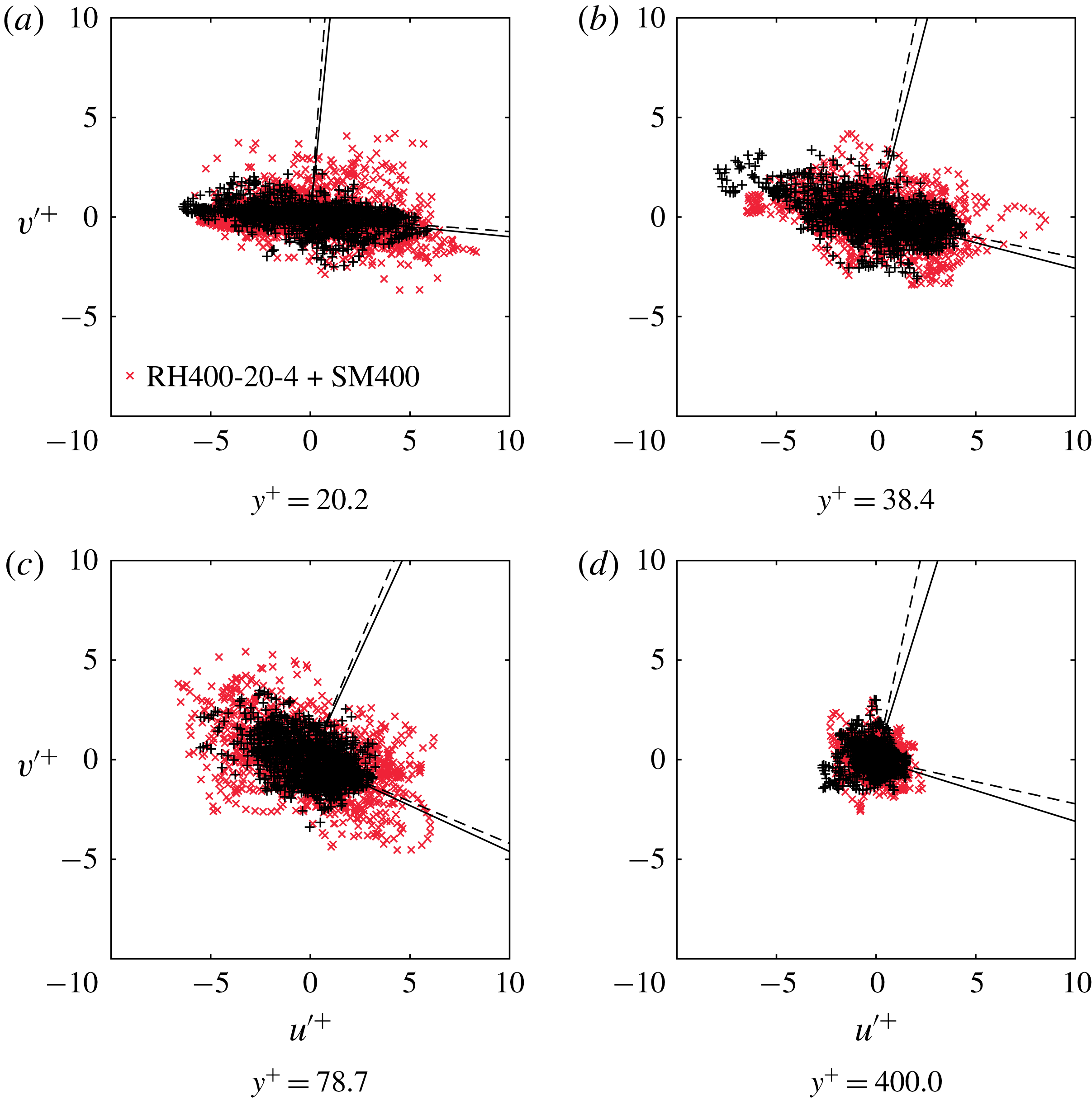
Figure 11. Distribution of $(u^{\prime +},v^{\prime +})$ at four wall-normal positions. Solid lines denote principal axes for SM400; dashed lines denote the principal axes for RH400-20-4.

The distributions of $(u^{\prime +},v^{\prime +})$ for both smooth- and rough-wall flow are illustrated in figure 11 at four wall-normal locations. These scatter plots illustrate differences in the intensity of coupled $u^{\prime }$ and $v^{\prime }$ events between smooth- and rough-wall flow, particularly in the near-wall region where roughness enhances the intensity of these velocity fluctuations and thus their contributions to the Reynolds shear stress. With increasing wall-normal position, these differences between smooth- and rough-wall flow subside. As noted above, the principal components in this plane are obtained by projecting the original velocity components onto the principal axes denoted by solid (smooth) and dashed (rough) lines in the scatter plots. Therefore, it is readily seen that the distribution of the principal components can be obtained by rotating the original distribution to the new coordinate system formed by the principal axes. While the principal components of smooth- and rough-wall flow presented here show slight deviations, the differences for all flow cases can be quantified by calculating the angle between the new coordinate system aligned with the principal components and the original coordinate system, denoted by $\unicode[STIX]{x1D719}$ , measured in the clockwise direction with respect to the streamwise direction. Then (6.15) is simply,

(6.17) $$\begin{eqnarray}\unicode[STIX]{x1D64C}^{T}=\unicode[STIX]{x1D63E}=\left[\begin{array}{@{}cc@{}}\cos \unicode[STIX]{x1D719} & -\text{sin}\unicode[STIX]{x1D719}\\ \sin \unicode[STIX]{x1D719} & \cos \unicode[STIX]{x1D719}\end{array}\right].\end{eqnarray}$$

Figure 12 presents the angle $\unicode[STIX]{x1D719}(\!\,^{\circ })$ as a function of wall-normal position for all flow cases. The angle varies almost linearly with wall-normal distance, reaching approximately $20^{\circ }$ near the centre of the log region. In the rough-wall cases, the angle of rotation for closely packed roughness elements ( $d/k=2$ case) is consistently reduced for all wall-normal positions as reflected in the RH400-20-2 trends. For the cases with larger element spacings ( $d/k=3$ – $4$ ), however, the magnitude is slightly larger than the smooth-wall cases near the roughness crest. Of note, all rough-wall cases approach the present $Re_{\unicode[STIX]{x1D70F}}=400$ smooth-wall trends in the outer layer, indicative of outer-layer similarity outside the roughness sublayer. However, the higher $Re$ smooth-wall flow of Hoyas & Jiménez (Reference Hoyas and Jiménez2006) has a lower value of $\unicode[STIX]{x1D719}$ in the log layer, indicating that this angle has $Re$ dependence. The effect of $Re$ on PCA clearly deserves more scrutiny.

7.1 Predictions of $u^{\prime }$ and $v^{\prime }$

Figure 13. Predictions of the Reynolds stresses for the smooth- and rough-wall cases involving $u^{\prime }$ and $v^{\prime }$ compared with the actual statistics from DNS. (a,c,e) Original model of Mathis et al. (Reference Mathis, Hutchins and Marusic2011) (7.1); (b,d,f) PCA-adapted models using $u_{OL}^{\prime +}$ (unrotated PCA-adapted model; open symbols) and the outer large-scale $\unicode[STIX]{x1D709}_{OL}^{\prime +}/\unicode[STIX]{x1D702}_{OL}^{\prime +}$ (consistent PCA-adapted model; filled symbols). Symbol $\times$ marks the reference location where the large-scale signal is extracted. Vertical lines denote the location of the roughness crest $k^{+}=20$ .

While the original model, i.e. (7.1), proposed by Mathis et al. (Reference Mathis, Hutchins and Marusic2011), focused on predicting the statistics of $u^{\prime }$ , it is possible to extend the model to other velocity components to make predictions of the full Reynolds stress tensor. Figure 13(a,c,e) compares the statistics of the Reynolds stresses calculated from DNS (lines) against those predicted by the original model (open symbols), where the outer large-scale signal $u^{\prime }$ is used for the calibration and prediction of both $u^{\prime }$ and $v^{\prime }$ in the near-wall region. Note that during the calibration for $v^{\prime }$ , the constants are determined using the near-wall large-scale components of $v^{\prime }$ . It is also found that the superposition coefficient for $v^{\prime }$ reaches only approximately 0.6 close to the reference location, as opposed to 1.0 for $u^{\prime }$ . It is not surprising that the predictions of the streamwise Reynolds stress, $\overline{u^{\prime 2}}$ , agree well with that calculated from DNS for both smooth and rough-wall flows. For the wall-normal, $\overline{v^{\prime 2}}$ , and shear, $\overline{u^{\prime }v^{\prime }}$ , stresses, however, the statistics are over-predicted by the original model as the reference plane is approached. Jiménez & Hoyas (Reference Jiménez and Hoyas2008) used spectral analysis to show that the presence of large-scale signatures with substantial energy are present in the premultiplied spectra of $u^{\prime }$ all the way from very near the wall to the top of the flow, a feature that represents the attached eddies whose dimensions scale well with the distance from the wall. Instead, spectra of $v^{\prime }$ and cospectra of $u^{\prime }v^{\prime }$ lack most of the energy carried by the long-wavelength structures residing in the outer layer, and thus embody the effects of detached eddies. The notion of attached and detached eddies, based on Townsend’s attached-eddy hypothesis (Townsend Reference Townsend1976), can be related to the predictive model in the sense that the outer large-scale information used as input in the model correlates better with $u^{\prime }$ rather than $v^{\prime }$ . This is seen in figure 13(c,e) with larger errors as the reference position is approached, since the outer layer is populated with more large-scale structures. Very recently, Yin et al. (Reference Yin, Huang and Xu2018) suggested that, while predicting the statistics of $v^{\prime }$ is accurate via the modulation effect embodied in the outer large-scale $u^{\prime }$ , the superposition constants should be determined by the outer large-scale $v^{\prime }$ . Following this idea, we have proposed an alternative model that calibrates each velocity component using the corresponding outer large-scale signal and compared to the model using only the large-scale $u^{\prime }$ . The predicted statistics are shown in appendix C and it is observed that the statistics of $v^{\prime }$ are improved at higher $Re$ with the alternative model but the correlations between $u^{\prime }$ and $v^{\prime }$ are still poorly reproduced.

Although the performance of the original model is limited by how well the outer large-scale signals are correlated with near-wall velocity signals, incorporating PCA to the model formulation allows one to make more robust predictions of the statistics for the Reynolds stresses associated with $u^{\prime }$ and $v^{\prime }$ ; at least, for the modest $Re$ we can effectively explore with the current DNS. Since the principal components are uncorrelated by construction, the modelling challenge is reduced to applying the analysis of AM to the principal components ( $\unicode[STIX]{x1D709}^{\prime }$ and $\unicode[STIX]{x1D702}^{\prime }$ ) themselves and to independently calibrating the predictive inner–outer model. Doing so yields two sets of calibrated coefficients and universal signals for the two principal components, respectively. Then, the predicted near-wall fluctuating principal components are readily obtained in analogy to (7.1), e.g.

(7.3) $$\begin{eqnarray}\displaystyle & \displaystyle \{\unicode[STIX]{x1D709}^{\prime +}(y^{+})\}_{p}=\unicode[STIX]{x1D709}^{\ast }(y^{+})\{1+\unicode[STIX]{x1D6FD}_{\unicode[STIX]{x1D709}}\unicode[STIX]{x1D709}_{OL}^{\prime +}(y_{O}^{+},\unicode[STIX]{x1D703}_{L\unicode[STIX]{x1D709}})\}+\unicode[STIX]{x1D6FC}_{\unicode[STIX]{x1D709}}\unicode[STIX]{x1D709}_{OL}^{\prime +}(y_{O}^{+},\unicode[STIX]{x1D703}_{L\unicode[STIX]{x1D709}}), & \displaystyle\end{eqnarray}$$

(7.4) $$\begin{eqnarray}\displaystyle & \displaystyle \{\unicode[STIX]{x1D702}^{\prime +}(y^{+})\}_{p}=\unicode[STIX]{x1D702}^{\ast }(y^{+})\{1+\unicode[STIX]{x1D6FD}_{\unicode[STIX]{x1D702}}\unicode[STIX]{x1D702}_{OL}^{\prime +}(y_{O}^{+},\unicode[STIX]{x1D703}_{L\unicode[STIX]{x1D702}})\}+\unicode[STIX]{x1D6FC}_{\unicode[STIX]{x1D702}}\unicode[STIX]{x1D702}_{OL}^{\prime +}(y_{O}^{+},\unicode[STIX]{x1D703}_{L\unicode[STIX]{x1D702}}). & \displaystyle\end{eqnarray}$$

From (6.12), the predicted velocity fluctuations are obtained by (dropping subscript $p$ for simplicity)

(7.5) $$\begin{eqnarray}\displaystyle \left.\begin{array}{@{}c@{}}u^{\prime }(y^{+})=c_{11}(y^{+})\unicode[STIX]{x1D709}^{\prime }(y^{+})+c_{21}(y^{+})\unicode[STIX]{x1D702}^{\prime }(y^{+}),\\ v^{\prime }(y^{+})=c_{12}(y^{+})\unicode[STIX]{x1D709}^{\prime }(y^{+})+c_{22}(y^{+})\unicode[STIX]{x1D702}^{\prime }(y^{+}),\end{array}\right\} & & \displaystyle\end{eqnarray}$$

where the coefficients $c_{ij}$ are obtained by calculating the eigenvectors of the covariance matrix at each wall-parallel plane near the wall, i.e. (6.15), of the velocity signals $u^{\prime }$ and $v^{\prime }$ extracted from the DNS data. Therefore, the Reynolds stresses can now be predicted according to

(7.6) $$\begin{eqnarray}\displaystyle \left.\begin{array}{@{}c@{}}\overline{u^{\prime 2}}=c_{11}^{2}\overline{\unicode[STIX]{x1D709}^{\prime 2}}+c_{21}^{2}\overline{\unicode[STIX]{x1D702}^{\prime 2}},\\ \overline{v^{\prime 2}}=c_{12}^{2}\overline{\unicode[STIX]{x1D709}^{\prime 2}}+c_{22}^{2}\overline{\unicode[STIX]{x1D702}^{\prime 2}},\\ \overline{u^{\prime }v^{\prime }}=c_{11}c_{12}\overline{\unicode[STIX]{x1D709}^{\prime 2}}+c_{21}c_{22}\overline{\unicode[STIX]{x1D702}^{\prime 2}}.\end{array}\right\} & & \displaystyle\end{eqnarray}$$

Note that the $\overline{\unicode[STIX]{x1D709}^{\prime }\unicode[STIX]{x1D702}^{\prime }}$ term does not appear in the expressions above since the principal components are orthogonal to each other by definition and this cross-correlation is thus zero.

The filled symbols in figure 13(b,d,f) represent the Reynolds stresses predicted using the principal components formulation described in (7.3) and (7.4), compared against the statistics calculated from DNS (lines). Overall, the predictions are in excellent agreement with the simulations for both smooth-wall (even in the higher $Re$ simulation of Hoyas & Jiménez (Reference Hoyas and Jiménez2006)) and the present rough-wall cases, including $\overline{v^{\prime }v^{\prime }}$ , and $\overline{u^{\prime }v^{\prime }}$ . Recall that the principal components are obtained by rotating the axes of $u^{\prime }$ and $v^{\prime }$ to the principal axes. Consequently, the large-scale information originally carried by $u_{OL}^{\prime +}$ is effectively transferred to both principal components. Therefore, this PCA-adapted model yields more consistent correlations between inner and outer signals compared to the original model as it embodies anisotropies inherent in the flow, resulting in improved predictions of statistics associated with $v^{\prime }$ .

In the formulation of the PCA-adapted model, the outer large-scale signals can be rotated by an angle that is either consistent with the outer principal components or with the near-wall principal components, e.g. $\unicode[STIX]{x1D719}(y_{O}^{+})$ or $\unicode[STIX]{x1D719}(y^{+})$ , respectively. These two sets of predictions are indistinguishable and are therefore not shown. The solid symbols in figure 13(b,d,f) as discussed above correspond to rotating the near-wall and outer-layer signals according to their local principal components – which can be quite different – so this formulation is termed the ‘consistent’ PCA-adapted model. Alternatively, one could still utilize the PCA-based model but instead leave the outer large-scale signals unrotated. Thus, the outer large-scale component of $u^{\prime }$ would be used to calibrate and predict the near-wall principal components $\unicode[STIX]{x1D709}^{\prime }$ and $\unicode[STIX]{x1D702}^{\prime }$ , respectively, and is termed the ‘unrotated’ PCA model. These results are also included in figure 13(b,d,f) and are represented by the open symbols. Interestingly, this variant of the model accurately predicts $\overline{u^{\prime }u^{\prime }}$ well, but results in considerable differences in other components with $Re$ . These differences are primarily due to poor correlation between the outer large-scale signal, $u^{\prime }$ , and the near-wall second principal component, $\unicode[STIX]{x1D702}^{\prime }$ .

Figure 14. As in figure 13, but for third-order statistical moments.

The efficacy of the PCA-adapted models is further investigated by examining higher-order statistics involving $u^{\prime }$ and $v^{\prime }$ , as shown in figures 14–17. These higher-order predictions are obtained in a similar fashion as the Reynolds stresses. In particular, third- (figures 14 and 16) and fourth-order (figures 15 and 17) moments, including cross-correlation terms, are computed using the original model of Mathis et al. (Reference Mathis, Hutchins and Marusic2011) (panels a and c of each figure) as well as both the consistent and unrotated PCA models (panels b and d of each figure), with the former represented by solid symbols and the latter by open symbols. As one would expect, predictions of $\overline{u^{\prime 3}}^{+}$ and $\overline{u^{\prime 4}}^{+}$ by all three models agree very well with the original statistics for the smooth- and rough-wall cases. However, as with $\overline{v^{\prime }v^{\prime }}^{+}$ , the original model poorly predicts $\overline{v^{\prime 3}}^{+}$ and $\overline{v^{\prime 4}}^{+}$ compared to the PCA-adapted models, although the consistent version provides the most accurate reconstruction of these $v^{\prime }$ statistics. Interestingly, all three models perform equally well in predicting the third-order cross-correlation ones. However, similar to the Reynolds shear stress, the fourth-order cross-terms are severely over-predicted by the original model and notably over-predicted by the unrotated PCA-based model, while the consistent PCA-based model accurately reconstructed these statistics. Finally, since the consistent PCA-adapted model is formulated for the specific purpose of accurately predicting near-wall statistics based on outer-layer information, it is not surprising to note small deviations in some of the higher-order statistics in the outer region for this model. Despite these outer-layer deviations, the consistent PCA-adapted model performs very well in predicting near-wall behaviour based on outer-layer flow information.

Figure 15. As in figure 13, but for fourth-order statistical moments.

Figure 16. As in figure 13, but for the third-order cross-correlated statistical moments.

Figure 17. As in figure 13, but for the fourth-order cross-correlated statistical moments.

7.2 Predictions of $w^{\prime }$

Figure 18. Two-point cross-correlation coefficient, $\unicode[STIX]{x1D70C}_{iO}(\unicode[STIX]{x0394}x^{+},\unicode[STIX]{x0394}z^{+})$ , between $w_{iL}$ and $u_{OL}$ in the $x$ – $z$ plane. Contour lines: case SM400 (dark lines: positive $\unicode[STIX]{x1D70C}_{iO}$ ; light lines: negative $\unicode[STIX]{x1D70C}_{iO}$ ) with increment/decrement of 0.2 times the peak values. Shaded contours: case SM2000 (light shade: positive $\unicode[STIX]{x1D70C}_{iO}$ ; dark shade: negative $\unicode[STIX]{x1D70C}_{iO}$ ). The outer plane is located at $y_{O}^{+}=100$ for SM400 and $y_{O}^{+}=200$ for SM2000. The inner plane is located at $y^{+}=20$ for both cases. Markers: ‘+’ denotes the positive peak and ‘ $\times$ ’ denotes the negative peak. Larger markers refer to the higher- $Re$ case.

The previous section was devoted to the prediction of joint statistics of $u^{\prime }$ and $v^{\prime }$ owing to their interdependence in wall turbulence. As shown in § 6.1 (figure 10), one can observe an important AM correlation between the near-wall $w^{\prime }$ and outer-layer  $u^{\prime }$ . Spectral analysis of $w^{\prime }$ (Jiménez & Hoyas Reference Jiménez and Hoyas2008) has shown that long-wavelength signatures are present over the entire flow thickness, although not as strong as $u^{\prime }$ , implying that $w^{\prime }$ is also an attached variable in the spirit of Townsend’s attached eddy hypothesis (Townsend Reference Townsend1976).

These observations, while important, are not sufficient to formulate a useful predictive model for statistics of $w^{\prime }$ . From the Reynolds stress balance equations, the only mechanism of production of $w^{\prime }$ fluctuations is the pressure strain, where it acts as a sink for $u^{\prime }$ and a source for $v^{\prime }$ and $w^{\prime }$ ; the net pressure strain, or the pressure dilatation, being zero in incompressible flow. This consequence complicates the situation because, for $w^{\prime }$ , the transport field (the source of its energy) is the pressure, which has long-range interactions and is difficult to model. Nevertheless, it is known that $p^{\prime }$ derives its intensity from $u^{\prime }$ , although it is not known which region in space and wavenumber predominantly contribute to it. Since near-wall statistics of $u^{\prime }$ can be inferred from the outer large-scale $u_{OL}^{\prime }$ , a major conclusion of AM, it make sense to directly consider the relationship between the near-wall $w^{\prime }$ and the outer-layer $u^{\prime }$ in more detail. To do so, we consider the two-point correlation between the near-wall $w^{\prime }$ and the outer-layer $u^{\prime }$ in the $x$ – $z$ plane with a two-point separation vector $(\unicode[STIX]{x0394}x^{+},\unicode[STIX]{x0394}z^{+})$ . This $x$ – $z$ correlation between $w^{\prime }$ on a near-wall plane ( $y_{i}^{+}$ ) and $u^{\prime }$ on an outer-layer plane ( $y_{O}^{+}$ ) is given by

(7.7) $$\begin{eqnarray}\unicode[STIX]{x1D70C}_{iO}(\unicode[STIX]{x0394}x^{+},\unicode[STIX]{x0394}z^{+};y_{i}^{+};y_{O}^{+})=\frac{\overline{w_{iL}^{\prime +}(x^{+},z^{+};y_{i}^{+})\quad u_{OL}^{\prime +}(x^{+}+\unicode[STIX]{x0394}x^{+},z^{+}+\unicode[STIX]{x0394}z^{+};y_{O}^{+})}}{\sqrt{\overline{w_{iL}^{\prime +}(x^{+},z^{+};y_{i}^{+})^{2}}}\sqrt{\overline{u_{OL}^{\prime +}(x^{+},z^{+};y_{O}^{+})^{2}}}}.\end{eqnarray}$$

Figure 18 presents iso-contours of this two-dimensional, off-plane, two-point correlation coefficient for the smooth-wall case SM400 in comparison with the higher- $Re$ smooth-wall case, SM2000. The inner plane is located at $y_{i}^{+}=20$ in both cases, while the outer reference location is $y_{O}^{+}=100$ for SM400 and $y_{O}^{+}=200$ for SM2000, respectively. An anti-symmetric correlation between $w_{iL}^{\prime }$ and $u_{OL}^{\prime }$ is noted in the $x$ – $z$ plane. Here the positive/negative peaks are no longer located along the $x$ -axis where $\unicode[STIX]{x0394}z^{+}=0$ , but with an offset in the spanwise direction whose distance increases with $Re$ . This spanwise offset is similar to the experimental results reported by Volino et al. (Reference Volino, Schultz and Flack2007) who also found that $u^{\prime }$ and $w^{\prime }$ in the same wall-parallel planes are correlated on both spanwise sides. The observed spanwise offset implies that, in order to extend the original model, equation (7.1), for $w^{\prime }$ statistics, one must calibrate the velocity component $w^{\prime }$ with both a streamwise and a spanwise shift. Thus, the original model can be modified as

(7.8) $$\begin{eqnarray}\{w^{\prime +}(y^{+})\}_{p}=w^{\ast }(y^{+})\{1+\unicode[STIX]{x1D6FD}_{w}u_{OL}^{\prime +}(y_{O}^{+},\unicode[STIX]{x1D703}_{x},\unicode[STIX]{x1D703}_{z})\}+\unicode[STIX]{x1D6FC}_{w}u_{OL}^{\prime +}(y_{O}^{+},\unicode[STIX]{x1D703}_{x},\unicode[STIX]{x1D703}_{z}),\end{eqnarray}$$

where $\unicode[STIX]{x1D703}_{x}$ and $\unicode[STIX]{x1D703}_{z}$ are the inclination angles in the streamwise and spanwise directions, respectively. For simplicity, $w^{\prime +}$ is calibrated with $u_{OL}^{\prime +}$ and not with $\unicode[STIX]{x1D709}_{OL}^{\prime +}$ or $\unicode[STIX]{x1D702}_{OL}^{\prime +}$ as the rotation angle of PCA is only relevant when considering cross-interactions, like those between $u^{\prime }$ and $v^{\prime }$ . Equivalent results are obtained if $\unicode[STIX]{x1D709}_{OL}^{\prime +}$ is used above instead.

Figure 19. Superposition coefficient $\unicode[STIX]{x1D6FC}_{w}$ (magnitude). Vertical line denotes the location of the roughness crest $k^{+}=20$ .

Although both the positive and negative peaks shown in figure 18 can be used to calibrate the model, for simplicity, only the negative peak is used herein. However, equivalent results can be obtained if the positive peak is used. The magnitude of the superposition coefficient for all flow conditions is shown in figure 19. Unlike the trends generally observed for $u^{\prime }$ , $|\unicode[STIX]{x1D6FC}_{w}|$ reaches a peak value (less than $1$ ) below the reference location and gradually diminishes further away from the wall. It is also seen that the superposition coefficient tends to grow as the $Re$ increases. Overall, consistent trends are observed between the smooth- and rough-wall flows at the same $Re$ , except that the peak values are increased and move closer to the reference location in the presence of roughness. Finally, the coefficient magnitude is reduced near the roughness crest with closely packed hemispheres compared to topographies with larger element spacings. Note that the superposition coefficients can be alternatively calibrated using the outer large-scale $w^{\prime }$ and the results and associated discussion can be found in appendix C.

Figure 20. Inclination angles $\unicode[STIX]{x1D703}_{x}$ and $\unicode[STIX]{x1D703}_{z}$ for $w^{\prime }$ . Vertical line denotes the location of the roughness crest $k^{+}=20$ .

Figure 20 shows the wall-normal evolution of the inclination angles $\unicode[STIX]{x1D703}_{x}$ and $\unicode[STIX]{x1D703}_{z}$ for $w^{\prime }$ in inner units. For the low $Re$ smooth-wall flow (SM400), $w_{iL}^{\prime +}$ appears to lag $u_{OL}^{\prime +}$ in the streamwise direction near the wall. Away from the wall, however, $w_{iL}^{\prime +}$ slowly transitions to lead $u_{OL}^{\prime +}$ in the streamwise direction as it approaches the reference location. In particular, $\unicode[STIX]{x1D703}_{x}$ for the case SM400 increases from an acute angle of approximately $45^{\circ }$ in the near-wall region to an obtuse one above $y^{+}\approx 40$ and eventually reaches $180^{\circ }$ close to the outer reference location. At higher $Re$ (SM2000), $w_{iL}^{\prime +}$ exhibits excellent synchronization with $u_{OL}^{\prime +}$ very close to the wall, but begins to lead $u_{OL}^{\prime +}$ with increasing wall-normal distance. Similar behaviours of $\unicode[STIX]{x1D703}_{x}$ are observed for the rough-wall cases; however, the $Re$ trend shown in the smooth cases is not as clear in the rough cases, at least for the moderate $Re$ studied herein. More interestingly, at the same $Re$ , $\unicode[STIX]{x1D703}_{x}$ near the roughness crest is gradually reduced for narrowly spaced roughness elements, but is indistinguishable between the smooth- and rough-wall cases if the elements are sufficiently far apart. This behaviour can be explained by the lifting effect of fluid away from the wall owing to the presence of roughness elements. The spanwise inclination angle, $\unicode[STIX]{x1D703}_{z}$ , is reported in figure 20(b). Here, $\unicode[STIX]{x1D703}_{z}$ decreases as a function of $y^{+}$ from approximately $50^{\circ }$ for the smooth-wall case SM400 and $40^{\circ }$ for SM2000 close to the wall, to $0^{\circ }$ near the reference plane. Unlike the trends observed in $\unicode[STIX]{x1D703}_{x}$ for the rough-wall cases, a $Re$ trend is more apparent in $\unicode[STIX]{x1D703}_{z}$ while the effect of roughness-element spacing diminishes.

Figure 21. Predictions of (a)  $\overline{w^{\prime 2}}^{+}$ and (b)  $\overline{w^{\prime 4}}^{+}$ for the smooth- and rough-wall cases in comparison with the original DNS statistics. Symbol $\times$ marks the reference location where the large-scale signal is extracted. Vertical line denotes the location of the roughness crest $k^{+}=20$ . Legend as in figure 13.

Figure 21 presents $\overline{w^{\prime 2}}$ and $\overline{w^{\prime 4}}$ using this modified model, equation (7.8), for both smooth- and rough-wall cases (note that $\overline{w^{\prime 3}}$ is zero by symmetry). Both $\overline{w^{\prime 2}}$ and $\overline{w^{\prime 4}}$ predicted by (7.8) are in good agreement with the DNS results for all surfaces. As these results are the initial attempt to model $w^{\prime }$ statistics with streamwise and spanwise offsets, definitive trends with $Re$ cannot be established owing to the relatively moderate $Re$ studied herein. However, the present results are clearly encouraging from a modelling perspective.

7.3 Model coefficients and universal signals in PCA form

Figure 22. Superposition coefficient, $\unicode[STIX]{x1D6FC}$ , inclination angle, $\unicode[STIX]{x1D703}_{L}$ , and modulation coefficient, $\unicode[STIX]{x1D6FD}$ , for the smooth- and rough-wall cases. (a,c,e) First principal component, $\unicode[STIX]{x1D709}^{\prime }$ ; (b,d,f) second principal component, $\unicode[STIX]{x1D702}^{\prime }$ . Vertical line denotes the location of the roughness crest $k^{+}=20$ .

The ‘consistent’ PCA-based model presented herein predicts the behaviour of the principal components, $\unicode[STIX]{x1D709}$ and $\unicode[STIX]{x1D702}$ , rather than the velocities as in the original model of Mathis et al. (Reference Mathis, Hutchins and Marusic2011) as shown in (7.3) and (7.4). Therefore, each principal component will have an associated superposition coefficient, $\unicode[STIX]{x1D6FC}$ , inclination angle, $\unicode[STIX]{x1D703}_{L}$ , and modulation coefficient, $\unicode[STIX]{x1D6FD}$ . These modelling coefficients are shown as a function of $y^{+}$ in figure 22, where the solid vertical line denotes the location of roughness crests ( $k^{+}=20$ ). For the first principal component, the superposition coefficient $\unicode[STIX]{x1D6FC}_{\unicode[STIX]{x1D709}}$ increases in the near-wall region from approximately $0.3$ for SM400 and $0.6$ for SM2000, respectively, to $1$ near the reference position. As $\unicode[STIX]{x1D6FC}_{\unicode[STIX]{x1D709}}$ is a measure of large-scale phenomena, the agreement noted between the smooth- and rough-wall cases implies that it is relatively unaffected by the presence of roughness, with a slight enhancement near the roughness crest as the element spacing increases. However, given the same roughness height and spacing, $\unicode[STIX]{x1D6FC}_{\unicode[STIX]{x1D709}}$ tends to grow with $Re$ . Similar trends are observed for $\unicode[STIX]{x1D6FC}_{\unicode[STIX]{x1D702}}$ , except for the lower magnitudes near the wall.

The inclination angle for the first principal component, $\unicode[STIX]{x1D703}_{L\unicode[STIX]{x1D709}}$ , varies slowly from $10^{\circ }$ to $25^{\circ }$ in the range $10<y^{+}<200$ in the highest $Re$ case, consistent with previous experiments (Mathis et al. Reference Mathis, Hutchins and Marusic2011). For lower $Re$ in both smooth- and rough-wall cases, however, this inclination angle increases with $y^{+}$ , reaching approximately $60^{\circ }$ close to the reference location. In addition, it is notable that roughness has no significant impact on $\unicode[STIX]{x1D703}_{L\unicode[STIX]{x1D709}}$ , except for the case with closely packed hemispheres (RH400-20-2) where $\unicode[STIX]{x1D703}_{L\unicode[STIX]{x1D709}}$ is consistently reduced compared to the smooth-wall case owing to the mutual sheltering of roughness elements. For the second principal component, $\unicode[STIX]{x1D703}_{L\unicode[STIX]{x1D702}}$ grows slower compared to $\unicode[STIX]{x1D703}_{L\unicode[STIX]{x1D709}}$ , reaching approximately $20^{\circ }$ for the highest $Re$ case and $30^{\circ }$ for lower $Re$ cases near the reference position. Roughly speaking, the behaviours of $\unicode[STIX]{x1D703}_{L\unicode[STIX]{x1D709}}$ and $\unicode[STIX]{x1D703}_{L\unicode[STIX]{x1D702}}$ are similar in the rough-wall cases, with the exception of the lowest $Re$ case, where the latter drops rapidly within the roughness sublayer.

A comparison of the modulation coefficients $\unicode[STIX]{x1D6FD}_{\unicode[STIX]{x1D709}}$ and $\unicode[STIX]{x1D6FD}_{\unicode[STIX]{x1D702}}$ is also shown in figure 22. Roughness enhances both $\unicode[STIX]{x1D6FD}_{\unicode[STIX]{x1D709}}$ and $\unicode[STIX]{x1D6FD}_{\unicode[STIX]{x1D702}}$ in the near-wall region compared to the smooth-wall result. At $Re_{\unicode[STIX]{x1D70F}}=400$ , roughness-element spacing appears to have a weak effect at best on $\unicode[STIX]{x1D6FD}_{\unicode[STIX]{x1D709}}$ and $\unicode[STIX]{x1D6FD}_{\unicode[STIX]{x1D702}}$ as the results for $d/k=2$ – $4$ show only small differences. In addition, $\unicode[STIX]{x1D6FD}_{\unicode[STIX]{x1D709}}$ and $\unicode[STIX]{x1D6FD}_{\unicode[STIX]{x1D702}}$ grow with $Re$ , as $\unicode[STIX]{x1D6FD}$ is another measure of the AM effect, which is the weakest in the $Re_{\unicode[STIX]{x1D70F}}=200$ case and strongest in the $Re_{\unicode[STIX]{x1D70F}}=600$ case among the rough-wall simulations. This effect seems to be stronger in $\unicode[STIX]{x1D6FD}_{\unicode[STIX]{x1D702}}$ .

Figure 23. Amplitude of the large-scale signals based on PCA for the smooth- and rough-wall cases. (a) First principal component, $\unicode[STIX]{x1D709}_{L}$ ; (b) second principal component, $\unicode[STIX]{x1D702}_{L}$ . Vertical line denotes the location of the roughness crest $k^{+}=20$ .

Figure 24. Statistical properties of the universal signals based on PCA for the smooth- and rough-wall cases. (a,c,e) First principal component, $\unicode[STIX]{x1D709}^{\ast }$ ; (b,d,f) second principal component, $\unicode[STIX]{x1D702}^{\ast }$ . Vertical line denotes the location of the roughness crest $k^{+}=20$ .

Note that the large-scale signals are the only terms in the predictive model that vary between the calibration and prediction processes. Thus, the correctness of the model depends significantly on the large scales themselves. If the amplitude of the large-scale signals are small compared to that of the universal signals, the agreement of the predictions reported herein might occur regardless of the correctness of the model. Therefore, the amplitude of the large-scale signals based on PCA are reported in figure 23 for the smooth- and rough-wall flows. For both principal components, it is shown that the amplitude of the large-scale signal approaches a constant value beyond $y^{+}\approx 100$ , consistent between the smooth- and rough-wall flows. Moreover, the amplitude of the large-scale signal decreases as the $Re$ increases and is likely to reach an asymptotic limit at sufficiently high $Re$ . This is expected as the separation of scales is difficult to achieve at low $Re$ and hence some proportion of the moderate- to large-scale structures are counted as the large scales while low-pass filtering the velocity signals. In comparison with the amplitude of the universal signals shown in figure 24(a,b), the large scales of both principal components remain non-negligible near the wall above the roughness crest. Therefore, the changes in the large-scale signals from the calibration to the prediction process have an impact on the predicted statistics based on the main model.

The effect of surface conditions on the variance, skewness and kurtosis (subtracted by 3) of the universal signals based on the principal components are shown in figure 24. The variance of the first principal component $\unicode[STIX]{x1D709}^{\ast }$ , normalized by the friction velocity, demonstrates a strong reduction in the peak values near the roughness crest, compared to the smooth-wall cases. This reduction is stronger for ‘k-type’ roughness as reflected in the cases with $d/k=3$ – $4$ compared to ‘d-type’ roughness as in the case with $d/k=2$ (closely packed hemispheres). Moreover, although all statistical properties of the first principal component are still $Re$ dependent among the rough-wall cases, they show perceivable tendency towards the high $Re$ limits in which the variance varies slowly while the skewness and kurtosis remain almost constant for $y^{+}>100$ for the smooth-wall flow at $Re_{\unicode[STIX]{x1D70F}}=2000$ . Even better outer-layer consistency is noted in the statistics of the second principal component, $\unicode[STIX]{x1D702}^{\ast }$ , where a similar tendency toward high $Re$ trends is present for the variance as well as excellent collapse of skewness and kurtosis observed among all cases beyond $y^{+}\approx 80$ . From the perspective of modelling the inner–outer interactions in rough-wall flows, this outer-layer similarity means it is conceivable that the universal signals calibrated at sufficiently high $Re$ , whether the surface is smooth or rough, can be used for reasonable predictions of the near-wall velocity signals outside the roughness sublayer based solely on the outer-layer large-scale information.

Figure 25. Energy spectra of the universal signals based on PCA at (a)  $y^{+}=k^{+}$ , (b)  $y^{+}=1.5k^{+}$ and (c)  $y^{+}=3k^{+}$ for the smooth- and rough-wall cases. All spectra are normalized by the friction velocity, $u_{\unicode[STIX]{x1D70F}}$ , and half-channel height, $h$ .

Energy spectra of the universal signals of the first principal component, $E_{\unicode[STIX]{x1D709}^{\ast }\unicode[STIX]{x1D709}^{\ast }}/hu_{\unicode[STIX]{x1D70F}}^{2}$ , at selected wall-normal positions are shown in figure 25. Very close to the roughness crest, at $y^{+}=20$ , large spikes are noted in the spectra of the rough-wall flows. The location of these energy spikes is closely related to the streamwise wavelength characterizing the geometry of the rough surfaces. For example, the first peak for the case RH400-20-4 corresponds to the wavelength $\unicode[STIX]{x1D706}=0.349$ , which is approximately equal to the separation between roughness elements ( $\sqrt{3}d$ or $4\sqrt{3}k$ ) in the streamwise direction (see the inset of figure 2(b) for a graphical representation of the geometry). Additionally, a higher degree of energy content is found at large wavenumbers in the rough-wall flows coupled with a reduction in energy at low wavenumbers compared to the smooth-wall case. This behaviour is expected since the presence of roughness energizes the near-wall turbulence, likely through the shedding of energetic, small-scale, vortical motions that scale with the roughness height. As one moves away from the wall, the effect of surface roughness is reduced, and, at $y^{+}=3k^{+}$ , all energy spectra at $Re_{\unicode[STIX]{x1D70F}}=400$ collapse onto one another, indicating that the influence of roughness is restricted to the roughness sublayer that resides within a few roughness heights from the wall. This collapse of energy spectra for all surface conditions is useful as a guideline for modelling turbulence over rough surfaces.