


1. Introduction
The last 20 years in cognitive science have been marked by what may be called a “Bayesian turn.” An increasing number of theories and methodological approaches either appeal to, or make use of, Bayesian methods (prominent examples include Clark, Reference Clark2013; Griffiths & Tenenbaum, Reference Griffiths and Tenenbaum2006; Knill & Pouget, Reference Knill and Pouget2004; Körding & Wolpert, Reference Körding and Wolpert2004; Oaksford & Chater, Reference Oaksford and Chater2001; Tenenbaum, Kemp, Griffiths, & Goodman, Reference Tenenbaum, Kemp, Griffiths and Goodman2011). The Bayesian turn pertains to both scientific methods for studying the mind, as well as to hypotheses about the mind's “method” for making sense of the world. In particular, the application of Bayesian formulations to the study of perception and other inference problems has generated a large literature, highlighting a growing interest in Bayesian probability theory for the study of brains and minds.
Probably the most ambitious and all-encompassing version of the “Bayesian turn” in cognitive science is the free energy principle (FEP). The FEP is a mathematical framework, developed by Karl Friston and colleagues (Friston, Reference Friston2010, Reference Friston2019; Friston, Daunizeau, Kilner, & Kiebel, Reference Friston, Daunizeau, Kilner and Kiebel2010; Friston, FitzGerald, Rigoli, Schwartenbeck, & Pezzulo, Reference Friston, FitzGerald, Rigoli, Schwartenbeck and Pezzulo2017a; Friston, Kilner, & Harrison, Reference Friston, Kilner and Harrison2006), which specifies an objective function that any self-organizing system needs to minimize in order to ensure adaptive exchanges with its environment. One major appeal of the FEP is that it aims for (and seems to deliver) an unprecedented integration of the life sciences (including psychology, neuroscience, and theoretical biology). The difference between the FEP and earlier inferential theories (e.g., Gregory, Reference Gregory1980; Grossberg, Reference Grossberg1980; Lee & Mumford, Reference Lee and Mumford2003; Rao & Ballard, Reference Rao and Ballard1999) is that not only perceptual processes, but also other cognitive functions such as learning, attention, and action planning can be subsumed under one single principle: the minimization of free energy through the process of active inference (Friston, Reference Friston2010; Friston et al., Reference Friston, FitzGerald, Rigoli, Schwartenbeck and Pezzulo2017a). Furthermore, it is claimed that this principle applies not only to human and other cognitive agents, but also self-organizing systems more generally, offering a unified approach to the life sciences (Friston, Reference Friston2013; Friston, Levin, Sengupta, & Pezzulo, Reference Friston, Levin, Sengupta and Pezzulo2015a).
Another appealing claim made by proponents of the FEP and active inference is that it can be used to settle fundamental metaphysical questions in a formally motivated and mathematically grounded manner, often using the Markov blanket construct that is the main focus of this paper. Via the use of Markov blankets, the FEP has been used to (supposedly) resolve debates about:
• the boundaries of the mind (Clark, Reference Clark, Metzinger and Wiese2017; Hohwy, Reference Hohwy, Metzinger and Wiese2017; Kirchhoff & Kiverstein, Reference Kirchhoff and Kiverstein2021),
• the boundaries of living systems (Friston, Reference Friston2013; Kirchhoff, Parr, Palacios, Friston, & Kiverstein, Reference Kirchhoff, Parr, Palacios, Friston and Kiverstein2018; van Es & Kirchhoff, Reference van Es and Kirchhoff2021),
• the life–mind continuity thesis (Kirchhoff, Reference Kirchhoff2018; Kirchhoff & van Es, Reference Kirchhoff and van Es2021; Wiese & Friston, Reference Wiese and Friston2021),
• the relationship between mind and matter (Friston, Wiese, & Hobson, Reference Friston, Wiese and Hobson2020; Kiefer, Reference Kiefer2020),
while also offering (apparently) new insights on:
• the (trans)formation and survival of social and societal organizations (Boik, Reference Boik2021; Fox, Reference Fox2021; Khezri, Reference Khezri2021),
• climate systems and planetary-scale self-organization and autopoiesis (Rubin, Parr, Da Costa, & Friston, Reference Rubin, Parr, Da Costa and Friston2020),
• the notions of “self” and “individual,” with studies on the sense of agency and on body ownership (Hafner, Loviken, Villalpando, & Schillaci, Reference Hafner, Loviken, Villalpando and Schillaci2020), (in utero) co-embodiment (Ciaunica, Constant, Preissl, & Fotopoulou, Reference Ciaunica, Constant, Preissl and Fotopoulou2021), pain experience (Kiverstein, Kirchhoff, & Thacker, Reference Kiverstein, Kirchhoff and Thacker2021), and symbiosis (Sims, Reference Sims2020),
• multi-level theories of sex and gender (Fausto-Sterling, Reference Fausto-Sterling2021), and
• ordering principles by which the spatial and temporal scales of mind, life, and society are linked (Hesp et al., Reference Hesp, Ramstead, Constant, Badcock, Kirchhoff and Friston2019; Ramstead, Badcock, & Friston, Reference Ramstead, Badcock and Friston2018; Veissière, Constant, Ramstead, Friston, & Kirmayer, Reference Veissière, Constant, Ramstead, Friston and Kirmayer2020) and possibly evolve (Poirier, Faucher, & Bourdon, Reference Poirier, Faucher and Bourdon2021).
The formalisms deployed by the FEP (as outlined in sect. 3 and 4 of this paper) are sometimes explicitly presented as replacing older (and supposedly outdated) philosophical arguments (Ramstead, Kirchhoff, Constant, & Friston, Reference Ramstead, Kirchhoff, Constant and Friston2019; Ramstead, Friston, & Hipólito, Reference Ramstead, Friston and Hipólito2020a), suggesting that they might be intended to serve as a mathematical alternative to metaphysical principles. A complicating factor here is that the core of the FEP rests upon an intertwined web of mathematical constructs borrowed from physics, computer science, computational neuroscience, and machine learning. This web of formalisms is developing at an impressively fast pace and the theoretical constructs it describes are often assigned a slightly unconventional meaning whose full implications are not always obvious. While this might explain some of its appeal, as it can seem to be steeped in unassailable mathematical justification, it also risks the possibility of “smuggling in” unwarranted metaphysical assumptions. Each new iteration of the theory also introduces novel formal constructs that can make previous criticisms inapplicable, or least require their reformulation (see e.g., the exchange between Seth, Millidge, Buckley, & Tschantz [Reference Seth, Millidge, Buckley and Tschantz2020]; Sun & Firestone [Reference Sun and Firestone2020a]; Van de Cruys, Friston, & Clark [Reference Van de Cruys, Friston and Clark2020]; as well as Sun & Firestone [Reference Sun and Firestone2020b]).
In this paper we want to focus on just one of the more stable formal constructs utilized by the FEP, namely the concept of a Markov blanket. Markov blankets originate in the literature on Bayesian inference and graphical modelling, where they designate a set of random variables that essentially “shield” another random variable (or set of variables) from the rest of the variables in the system (Bishop, Reference Bishop2006; Murphy, Reference Murphy2012; Pearl, Reference Pearl1988). By identifying which variables are (conditionally) independent from each other, they help represent the relationships between variables in graphical models, which serve as useful and compact graphical abstractions for studying complex phenomena. By contrast, in the FEP literature Markov blankets are now frequently assigned an ontological role in which they either represent, or are literally identified with, worldly boundaries. This discrepancy in the use of Markov blankets is indicative of a broader tendency within the FEP literature, in which mathematical abstractions are treated as worldly entities. By focusing here on the case of Markov blankets, we hope to give a specific diagnosis of this problem, and then a suggested solution, but our analysis does also have potentially wider implications for the general use of formal constructs in the FEP literature, which we think are often described in a way that is crucially ambiguous between a literalist, a realist, and an instrumentalist reading (see Andrews [Reference Andrews2020] and van Es [Reference van Es2021] for broader reviews of these kinds of issues in the FEP literature).
In order to give a comprehensive picture of where the field is now, we need to first go back to basics and explain some fundamental concepts. We will therefore start our paper by tracing the development of Markov blankets in section 2, beginning with their standard application in graphical models (focusing on Bayesian networks) and probabilistic reasoning, and including some of the formal machinery required for variational Bayesian inference. In section 3 we present the active inference framework and the different roles played by Markov blankets within this framework, which we suggest has ended up stretching the original concept beyond its initial formal purpose (here we distinguish between the original “Pearl” blankets and the novel “Friston” blankets). In section 4 we focus specifically on the role played by Friston blankets in distinguishing the sensorimotor boundaries of organisms, which we argue stretches the original notion of a Markov blanket in a potentially philosophically unprincipled manner. In section 5 we discuss some conceptual issues to do with Friston blankets, and in section 6 we suggest that it would be both more accurate and theoretically productive to keep Pearl blankets and Friston blankets clearly distinct from one another when discussing active inference and the FEP. This would avoid conceptual confusion and also disambiguate two distinct theoretical projects that might each be valuable in their own right.
2. Probabilistic reasoning and Bayesian networks
The concept of a Markov blanket was first introduced by Pearl (Reference Pearl1988) in the context of his work on probabilistic reasoning and graphical models. In this section we will introduce the formal background that is required in order to understand the role played by Markov blankets in this literature. This will provide the necessary foundation for sections 3 and 4, where we will discuss the ways in which Markov blankets have been used (and potentially misused) within the FEP literature.
2.1 Probabilistic reasoning
Probabilistic reasoning is an approach to formal decision making under uncertain conditions. This approach is typically introduced as a middle ground between heuristics-based systems that are fast but will face many exceptions, and rules-based systems that will be accurate but slow and hard to put into practice. The probabilistic reasoning framework is a way to summarize relevant exceptions, providing a middle ground between speed and accuracy. The first step in this approach is to classify variables in order to distinguish between observables and unobservables. Inference is then the process by which one can estimate an unobservable given some observables. For instance, how is it that we are able to determine if a watermelon is ripe by knocking on it? On the basis of observing the sound (resonant or dull), we are able to infer the unobserved state of the watermelon (ripe or not). When formalizing such kinds of everyday inference problems, we need to answer three interrelated questions:
(1) How do we adequately summarize our previous experience?
(2) How do we use previous experience to infer what is going on in the present?
(3) How do we update the summary in the light of new experience?
In section 2.2 we will address Bayesian networks, a specific way of answering question 1. In section 2.3 we will address variational inference, a specific way of addressing question 2. Question 3 is addressed by appealing to Bayes theorem. Bayes theorem normally takes the following form:

This formula is a recipe for calculating the posterior probability, p(x|y), of an unobserved set of states x ∈ X given observations y ∈ Y. The probability p(x) captures prior knowledge about states x (i.e., a prior probability), while p(y|x) describes the likelihood of observing y for a given x. The remaining term, p(y), represents the probability of observing y independently of the hidden state x and is usually referred to as the marginal likelihood or model evidence, and plays the role of a normalizing factor that ensures that the posterior sums up to 1. In other words, the posterior probability p(x|y) represents the optimal combination of prior information represented by p(x) (e.g., what we know about ripe watermelons, before we get to knock on the one in front of us) and a likelihood model p(y|x) of how observations are generated in the first place (e.g., how watermelons give rise to different sounds at specific maturation stages, including the observed sound y), normalized by the knowledge about the observations integrated over all possible hidden variables, p(y) (e.g., how watermelons may typically sound, regardless of the specific maturation stage).
What holds for everyday reasoning problems holds for cognition and science as well: how can a cognitive system estimate the presence of some object on the basis of the state of its receptors alone? How can a neuroscientist estimate brain activity on the basis of magnetic fields measured in an fMRI scanner? Both of these kinds of questions can be formalized using Bayes' theorem (see e.g., Friston, Harrison, & Penny, Reference Friston, Harrison and Penny2003; Gregory, Reference Gregory1980; Penny, Friston, Ashburner, Kiebel, & Nichols, Reference Penny, Friston, Ashburner, Kiebel and Nichols2011).
Although this scheme offers a powerful tool for probabilistic inference, it is mostly limited to simple, low-dimensional, and often discrete or otherwise analytically tractable problems. For example, computing the exact model evidence is rarely feasible, because the computation is often analytically intractable or computationally too expensive (Beal, Reference Beal2003; Bishop, Reference Bishop2006; MacKay, Reference MacKay2003). To obviate some of the limitations of exact Bayesian inference schemes, different approximations can be deployed, which rely on either stochastic or deterministic methods. In this context, variational methods (Beal, Reference Beal2003; Bishop, Reference Bishop2006; Blei, Kucukelbir, & McAuliffe, Reference Blei, Kucukelbir and McAuliffe2017; Hinton & Zemel, Reference Hinton and Zemel1994; Jordan, Ghahramani, Jaakkola, & Saul, Reference Jordan, Ghahramani, Jaakkola and Saul1999; MacKay, Reference MacKay2003; Zhang, Bütepage, Kjellström, & Mandt, Reference Zhang, Bütepage, Kjellström and Mandt2018) are a popular choice, including for the FEP framework discussed in this paper. We will discuss those in section 2.3, but first we will introduce the Bayesian network approach developed by Pearl.
2.2 Bayesian networks
Pearl (Reference Pearl1988) developed a mathematical language to formulate summaries of previous experience in computer learning systems. That mathematical language constitutes the focus of this paper, due to the ease with which it can be used to demonstrate the use (and misuse) of Markov blankets using probabilistic graphical models. Probabilistic graphical models capture the dependencies between random variables using a visual language that renders the study of certain probabilistic interactions across variables, traditionally defined with analytical methods, more intuitive and easy to track.Footnote 1 Random variables are drawn as nodes in a graph, with shaded nodes usually representing variables that are observed and empty nodes used for variables that are unobserved (latent or hidden variables). The (probabilistic) relationships between such random variables are then expressed using edges (lines) connecting the nodes. For present purposes we will focus on acyclic graphs with directed edges, which provide the basis for graphical models, and play a crucial role in the context of active inference (Friston, Parr, & de Vries, Reference Friston, Parr and de Vries2017b). Relationships between the variables are often described using genealogical terms, with pa(a) being the parents (or “ancestors”) of their children (or “descendants”) node a and copa(a) being the co-parents: nodes with which a has a child in common. In Figure 1 below, m is the target variable, c and b are the parents of m, a is the child of m, and e is m's co-parent since they have a in common as a child. Although the dependencies are formally defined in terms of basic manipulations on probability distributions, graphical models provide some practical advantages in reasoning about these formal properties, presenting a clear and easily interpretable depiction of the relationships between variables.

Figure 1. The “alarm” network with examples of Markov Blankets for two different variables. The target variables are indicated with a dashed pink circle, while the variables that are part of the Markov blanket are indicated with a solid pink circle.
Let us introduce a simple textbook example that will help familiarize us with some of the nuances of Bayesian graphs. The illustration we will consider is a slight modification of a common textbook example, the “alarm” network (Pearl, Reference Pearl1988). Imagine that you have an alarm system (a) in your house and it is sensitive to motion, so that it will go off whenever it detects any movement (m). In some cases the movement can be caused by a burglar (b), but it could also be caused by your neighbour's cat (c). The alarm is also sensitive (for independent reasons) to power surges in the electrical grid, and can sometimes be triggered by changes in the supply of electricity (e). Of course, having an alarm is not much help when you're away, so you asked two of your neighbours – Gloria (g) and John (j) – to call you if they hear the alarm. Unfortunately, John suffers from severe tinnitus (t) and has been known to call you even though the alarm wasn't on. This example can be formalized both algebraically and visually.
Algebraically, this example can be expressed by the following joint probability of all the included variables:

This joint probability is not especially easy to interpret. The graph in Figure 1 models the dependencies among the variables in this scenario in a more easily interpretable manner, where directed edges indicate probabilistic relationships between nodes (variables).
The alarm network allows us to illustrate a number of canonical examples of statistical (in)dependencies between nodes, known also as d-separation (Pearl, Reference Pearl1988):
• e and m are marginally independent but only conditionally dependent if a is observed (i.e., when a becomes a shaded node), a case technically known also as head-to-head relation. This can be made intuitive in the following way: in general, surges in electricity e and other forms of movement m are not related to one another. Once you know that the alarm went off, then knowing that there was no surge implies that some other factor was responsible for the activation (and vice versa).
• c and a are marginally dependent but conditionally independent if m is observed, also known as head-to-tail. Once you know that there was movement, knowing that the cat caused the movement will not make a difference in your estimation for whether the alarm went off.
• g and j are marginally dependent but conditionally independent if a is observed, also known as tail-to-tail. In general, Gloria calling will make it likely that John will call as well. But once you know the alarm went off, Gloria calling will not change the probability of John calling.
Bayesian networks like the one above play an especially prominent role in exemplifying marginal and conditional independence relations. Marginal independence is represented by the lack of a directed path between two nodes. Conditional independence is defined in terms of a node “shielding” one variable (or set of variables) from another node. This notion of “shielding” can be made more explicit by introducing the idea of a Markov blanket, which will be the central focus of this paper.
A Markov blanket designates the minimalFootnote 2 set of nodes with respect to which a particular node (or set of nodes) is conditionally independent of all other nodes in a Bayesian graph,Footnote 3 that is, it shields that node from all other nodes. Formally, a Markov blanket for a set of variables x i is thus equivalent to:

where pa(x i) corresponds to the parents of x i, ch(x i) to the children, and copa(x i) to the co-parents of x i respectively.
To make the notion of a Markov blanket clearer, we have drawn the blankets of different nodes in the alarm network. Figure 1a shows the Markov blanket for node m or mb(m). It is composed of m's parents (c and b), its child (a), and its children's other parents (e). The mb(j) shown in Figure 1b, on the other hand, is composed of just two nodes (a and t), hence:

What this means intuitively is that given the Markov blanket of a node, any other change in the network will not make a direct difference to one's estimation of the random variable. If you could know John's state of tinnitus and the state of the alarm, you can calculate the probability that he will be calling. The rest of the state of the network does not make a difference for this calculation. In other words, a node's Markov blanket captures exactly all nodes that are relevant to infer the state of that node. As we will illustrate in the next section, the conditional independence of any variable from the nodes outside its Markov blanket is one of the key factors that makes probabilistic graphs useful for inference.
2.3 Variational inference
We mentioned before that exact Bayesian inference will in many cases not be feasible. There are a number of techniques available in the literature to perform approximate inference. The version of approximate inference that we will focus on in this paper is called variational inference, and here Markov blankets play an important role in identifying which variables are actually relevant to any given inference problem.
The main idea behind variational inference is that the problem of inferring the posterior probability of some latent or hidden variables from a set of observations can be transformed into an optimization problem. Roughly speaking, the method involves stipulating a family Q of probability densities over the latent variables, such that each q(x) ∈ Q is a possible approximation to the exact posterior. The goal of variational inference is then to find an optimal distribution q*(x) that is closest to the true posterior. The candidate distribution is often called the recognition or variational density, because the methods used employ variational calculus, that is, functions q(x) are varied with respect to some partition of the latent variables in order to achieve the best approximation of p(x|y). This measure of closeness is formalized by the Kullback–Leibler divergence, a common measure of dissimilarity between two probability distributions (here denoted by D KL):

Equation (5) reads: the optimal distribution is the one that minimizes the dissimilarity between the variational density and the exact posterior. This can be shown to be bounded (above) by the minimization of a quantity that is called variational free energy (see Bishop, Reference Bishop2006; Murphy, Reference Murphy2012):

One of the most crucial components of variational inference is the choice of a family Q. If the chosen Q is too complicated, then the inference will remain unfeasible, but if it is too simple then the optimal distribution might be too far removed from the exact posterior. Popular choices for Q include a treatment in terms of conjugate priors (Bishop, Reference Bishop2006), a mean-field approximation (Parisi, Reference Parisi1988), the variational Gaussian approximation (Opper & Archambeau, Reference Opper and Archambeau2009), and the Laplace method (MacKay, Reference MacKay2003).
It is however crucial to highlight that such methods operate only on the family Q of the variational density q(x). This means that they do not necessarily encode dependencies capturing constraints among variables x i ∈ x derived from knowledge of the underlying system to be modelled (e.g., its physics). These further constraints are instead captured in the joint probability p(y, x), used to infer x via the posterior p(x|y), of which q(x) is an approximation (see equation [6]). It is here that the concepts of marginal and conditional independence show up again. Inferential processes can in fact be simplified by orders of magnitude if we consider that each variable will only exert some (direct) influence on a number of (other) variables that is usually quite limited.
In the mean-field approach, for example, mean-field effects (i.e., averages) for a particular partition (i.e., a subset) of variables are constructed only using its Markov blanket (Jordan et al., Reference Jordan, Ghahramani, Jaakkola and Saul1999). This means that such partition need only be optimized with respect to its blanket states, hence the idea of “shielding,” intended to highlight how only a relatively small number of variables need actually be considered in most problems of inference (Bishop, Reference Bishop2006; Murphy, Reference Murphy2012). In more concrete terms, and using our previous example of the alarm network, to infer the most likely cause that set off the alarm one need not consider burglary (b) directly, as the effects of this variable are already captured by motion (m). Likewise, when trying to infer if John (j) will have to call us, we need to only consider if the alarm was actually set off, regardless of whether it was because of some electricity supply problem (e) or some motion detected by the alarm (m), or whether John's tinnitus (t) is the true cause of John's call. Through an iterative procedure in which each (subset of) node(s) is optimized given its Markov blanket, the process will settle on the best estimate of the posterior distribution given the simplifying assumptions that were made for a particular model. As we can see by now, Markov blankets are a relatively technical construct traditionally applied to problems of inference.
2.4 Bayesian model selection
One of Pearl's main innovations when it comes to Bayesian networks was the idea that dependencies between different variables of the original system could be discovered by manipulating (i.e., “intervening on”) a chosen variable and seeing which other variables are affected. This idea has proven to be immensely useful when trying to infer the organization of some system with an unknown structure, that is, for structure learning, or structure discovery. Historically, however, other distinct approaches have also been adopted to tackle this problem. For example, structure learning can be utilized either with or without the causal assumptions advocated by Pearl and others (see Vowels, Camgoz, & Bowden [Reference Vowels, Camgoz and Bowden2021] for a recent review). In this family of methods, the class of score-based approaches (Vowels et al., Reference Vowels, Camgoz and Bowden2021) is of particular interest to this paper given its tight relations to the FEP and the use of Markov blankets. In score-based approaches, to discover the values and relations between variables one simply constructs multiple (classes of) models of the system under investigation and compares them to determine which one of them makes the most accurate predictions about the observable data.
This process of pitting models against each other is often referred to as (possibly Bayesian) model selection (Penny et al., Reference Penny, Friston, Ashburner, Kiebel and Nichols2011; Stephan, Penny, Daunizeau, Moran, & Friston, Reference Stephan, Penny, Daunizeau, Moran and Friston2009). Importantly, while this process optimizes for how well different models fit the data, it also keeps track of the tradeoff between model accuracy and model complexity. For example, it is clear that the alarm network we discussed before could have been more complex: either Gloria's or John's telephone batteries might play a role in whether they phone you or not, perhaps there are other ways in which the alarm might be triggered, and so on. However, the inclusion of such information in the network would have further complicated the graph without necessarily making it more accurate as a modelling tool (at least relative to our purposes).
What then decides the level of complexity that a good Bayesian model should have? Is it one that captures all the possibly relevant facts that might make a difference, or is it the simplest one that still makes a good enough prediction? The dominant assumption in the literature is that there is a tradeoff between making a model fit the data as closely as possible and that model's ability to predict new data points. In other words, the best model is one that accounts for the available data in the most parsimonious way (Friston et al., Reference Friston, Parr and de Vries2017b; Penny et al., Reference Penny, Friston, Ashburner, Kiebel and Nichols2011; Stephan et al., Reference Stephan, Penny, Daunizeau, Moran and Friston2009). This intuition can be formalized via a process of model comparison using different criteria, for example, the Akaike information criterion, the Bayesian information criterion, or variational free energy (via the maximization of model evidence, equivalent to the minimization of surprisal), but there is a general agreement that Bayesian methods offer a quantification of Occam's razor (Jefferys & Berger, Reference Jefferys and Berger1991). In the case of variational free energy, one can then take into account a trade-off between the complexity of a model and the accuracy with which it is able to predict the data (or observations). When minimizing free energy using a range of different models, the one with the lowest free energy is thus taken to be the one that accounts for the data in the most parsimonious way (cf. the Occam factor discussed by Bishop, Reference Bishop2006; Daunizeau, Reference Daunizeau2017; Friston, Reference Friston2010; MacKay, Reference MacKay2003).
It is therefore important to note that the basic epistemic aim (even for the models used in the context of active inference) is not to arrive at a complete model of the system under investigation, but rather to obtain the most parsimonious model that accurately captures the relevant relations (Baltieri & Buckley, Reference Baltieri and Buckley2019; Stephan et al., Reference Stephan, Penny, Moran, den Ouden, Daunizeau and Friston2010). This complexity/accuracy trade-off is important to prevent overfitting the model to the available data.
Of course, which facts are relevant depends on the questions we ask: if we are interested in how an alarm can be sensitive to both motion and changes in electric current, the model drawn in Figure 1 might not be very helpful, but it would do just fine for the purpose of estimating (i.e., inferring) the probability that your house is really being robbed when your tinnitus-struck neighbour calls you to report a ringing noise. There is therefore a sense in which model selection is influenced by pragmatic considerations. By choosing the data worth considering for their analysis, the scientist chooses their level of analysis, and by choosing which dimensions in model space are relevant to answer their question, the scientist chooses what models (or families of models) to consider (Penny et al., Reference Penny, Friston, Ashburner, Kiebel and Nichols2011; Stephan et al., Reference Stephan, Penny, Moran, den Ouden, Daunizeau and Friston2010). The same phenomenon can be analysed using different sources of data. For example, in a study of decision making one can include only behavioural data, or add neural measurements as well. The choice of relevant dimensions in model space is often influenced by previous empirical evidence, meaning that relevant factors and model spaces themselves should be updated as new evidence becomes available. Clearly these considerations are not unique to (Bayesian) model selection. Furthermore, they don't negate any of its merits, but rather simply highlight the requirement for pragmatic constraints in solving difficult problems with infinitely large model spaces, especially in realistic situations and away from hypothetical ideal observer scenarios.
2.5 Taking stock
We have introduced a number of concepts and constructs that jointly form a toolkit for Bayesian inference: Bayesian networks can provide problem-specific summaries of the available data that predict the probability of future observations. Variational inference provides an elegant method to replace an intractable inference problem with a tractable optimization problem. Variational methods of the kind we have described in this section have been employed across the sciences. In this scientific context, Markov blankets are an auxiliary technical concept that demarcate what additional nodes are relevant for estimating the state of a specific target node.
This technical concept of a Markov blanket has undergone a significant transformation in the literature on the FEP. In order to distinguish this original Markov blanket concept from the one that we will draw out of the FEP literature in section 4, we will, with apologies to Judea Pearl, refer to instances of the original concept as “Pearl blankets” throughout the rest of the paper. The novel Markov blanket concept introduced in section 4, on the other hand, we will refer to as a “Friston blanket.”Footnote 4
3. Pearl blankets in the active inference framework
The specific application of the FEP that we will focus on here is the active inference framework. In active inference, the concepts of variational inference are applied to living systems. The thought is that living systems are in the same position as data scientists. They “observe” the activity at their sensory receptors and need to infer the state of the world. However, the framework goes even further and postulates that living systems need to also act on the world so as to stay within viable bounds, as merely inferring the states of the environment cannot guarantee survival (this idea is illustrated in Fig. 2). In this section we will introduce the way that Pearl blankets are used for modelling purposes in the active inference literature and highlight one initial conceptual issue with this use.
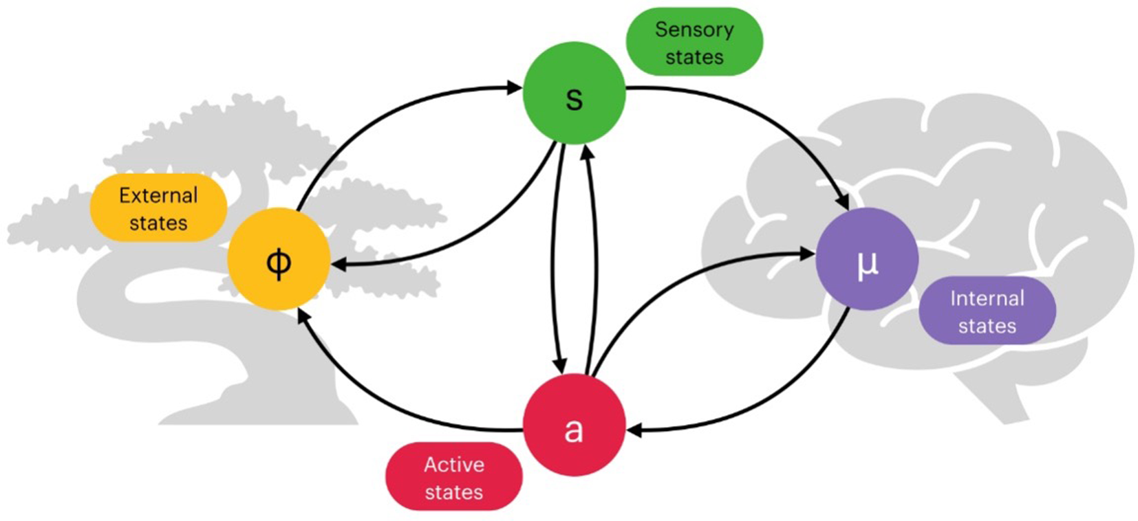
Figure 2. The Markov blanket as a sensorimotor loop (adapted from Friston, Reference Friston2012). A diagram representing possible dependences between different components of interest: sensory states (green), internal states (violet), active states (red), and external states (yellow). Notice that although this figure uses arrows to signify directed influences, the diagram is not a Bayesian network as it depicts different sets of circular dependences (between pairs of components, and an overall loop including all nodes).
3.1 Modelling active inference with Pearl blankets
Active inference is a process theory derived from the application of variational inference to the study of biological and cognitive systems (Friston, Reference Friston2013, Reference Friston2019; Friston et al., Reference Friston, Daunizeau, Kilner and Kiebel2010, Reference Friston, Rigoli, Ognibene, Mathys, Fitzgerald and Pezzulo2015b, Reference Friston, FitzGerald, Rigoli, Schwartenbeck and Pezzulo2017a). The core assumption underlying active inference is that living organisms can be thought of as systems whose fundamental imperative is to minimize free energy (this constitutes the so-called free energy principle). Active inference attempts to explain action, perception, and other aspects of cognition under the umbrella of variational (and expected) free energy minimization (Feldman & Friston, Reference Feldman and Friston2010; Friston et al., Reference Friston, Daunizeau, Kilner and Kiebel2010, Reference Friston, FitzGerald, Rigoli, Schwartenbeck and Pezzulo2017a). From this perspective, perception can be understood as a process of optimizing a variational bound on surprisal, as advocated by standard methods in approximate Bayesian inference applied in the context of perceptual science (see for instance Dayan, Hinton, Neal, and Zemel, Reference Dayan, Hinton, Neal and Zemel1995; Friston, Reference Friston2005; Knill & Richards, Reference Knill and Richards1996; Lee & Mumford, Reference Lee and Mumford2003; Rao & Ballard, Reference Rao and Ballard1999). At the same time, action is conceptualized as a process that allows a system to create its own new observations, while casting motor control as a form of inference (Attias, Reference Attias, Bishop and Frey2003; Kappen, Gómez, & Opper, Reference Kappen, Gómez and Opper2012), with agents changing the world to better meet their expectations.
Active inference integrates a more general framework where minimizing expected free energy accounts for more complex processes of action and policy selection (Friston et al., Reference Friston, Rigoli, Ognibene, Mathys, Fitzgerald and Pezzulo2015b, Reference Friston, FitzGerald, Rigoli, Schwartenbeck and Pezzulo2017a; Tschantz, Seth, & Buckley, Reference Tschantz, Seth and Buckley2020). Expected free energy is the free energy expected in the future for unknown (i.e., yet to be seen) observations, combining a trade-off between (negative) instrumental and (negative) epistemic values. A full treatment of active inference remains beyond the scope of this manuscript (for some technical treatments and reviews, see e.g., Biehl, Guckelsberger, Salge, Smith, & Polani, Reference Biehl, Guckelsberger, Salge, Smith and Polani2018; Bogacz, Reference Bogacz2017; Buckley, Kim, McGregor, & Seth, Reference Buckley, Kim, McGregor and Seth2017; Da Costa et al., Reference Da Costa, Parr, Sajid, Veselic, Neacsu and Friston2020; Friston et al., Reference Friston, Parr and de Vries2017b; Sajid, Ball, Parr, & Friston, Reference Sajid, Ball, Parr and Friston2021), but we wish to highlight the formal connection between this framework and the use of variational Bayes in standard treatments of approximate probabilistic inference (as described in the previous section). Acknowledging this relationship is crucial if we want to understand the role Pearl blankets might play in active inference.
To understand the role played by Pearl blankets in active inference, we first need to identify some of the formal notation used by active inference, which is related to the variational approaches described in the previous section. Here we use the notation previously adopted in equation (6), while also introducing a second, distinct, set of hidden random variables: action policies π ∈ Π, sequences of control states u ∈ U up to a given time horizon τ with 0 ≤ τ ≤ T, that is, $\pi = [ {u_1, \;u_2, \;\;\ldots , \;\;u_\tau } ]$ . This will allow us to formulate perception and action as variational problems in active inference. Perception is the minimization (at each time step t)Footnote 5 of the following equation:

In other words: at each time step t, select the variational density that minimizes free energy. Action is then characterized (at each time step t) in terms of control states u where:

and with the (approximate) prior on a policy π, q(π), defined as

This describes action selection as a minimization of what is called expected free energy, G(π, τ), based on beliefs about future and unseen observations y, up to a time horizon τ ≤ T. In other words, at each time step t, select the policy π that you expect will minimize free energy a number of time steps τ into the future (for a more detailed treatment, see one of the latest formulations found in, e.g., Da Costa et al., Reference Da Costa, Parr, Sajid, Veselic, Neacsu and Friston2020; Sajid et al., Reference Sajid, Ball, Parr and Friston2021).
In doing so, we can notice that equation (7) essentially mirrors the previously defined equation (6), with the important caveat that in active inference sequences of control states (i.e., policies π) are now a part of the free energy F (this is conceptually similar to other formulations of control as inference, such as Attias, Reference Attias, Bishop and Frey2003; Kappen et al., Reference Kappen, Gómez and Opper2012).Footnote 6 In a closed loop of action and perception, policies π can effectively modify the state of the world, generating new observations y, something that classical formulations of variational inference in statistics and machine learning do not consider, instead assuming fixed observations or data (Beal, Reference Beal2003; Bishop, Reference Bishop2006; MacKay, Reference MacKay2003).
Some formulations of active inference, especially the earlier ones (Friston, Reference Friston2008; Friston, Mattout, Trujillo-Barreto, Ashburner, & Penny, Reference Friston, Mattout, Trujillo-Barreto, Ashburner and Penny2007; Friston, Trujillo-Barreto, & Daunizeau, Reference Friston, Trujillo-Barreto and Daunizeau2008), have explicitly relied on a set of assumptions similar to the ones mentioned in the previous section: a mean-field approximation and the use of Pearl blankets to shield nodes. As mentioned in section 2.3 (see also Jordan et al., Reference Jordan, Ghahramani, Jaakkola and Saul1999), Pearl blankets can be used to simplify the minimization of variational free energy by specifying which variables need to be considered for mean-field averages via appropriate constraints of conditional independence. Works such as Friston et al. (Reference Friston, Mattout, Trujillo-Barreto, Ashburner and Penny2007), Friston et al. (Reference Friston, Trujillo-Barreto and Daunizeau2008), and Friston (Reference Friston2008), however, make use of a “structured” mean-field assumption,Footnote 7 where variables are partitioned in three independent sets: hidden states and inputs, parameters, and hyper-parameters. In this case, the use of Pearl blankets is entirely consistent with existing literature and definitions of conditional independence in graphical models, albeit slightly unnecessary given the relatively low number of partitions. Indeed, it is not entirely clear what Pearl blankets actually add to this formulation, since it is often claimed that given a partition of variables (out of three) “the Markov [ = Pearl] blanket contains all [other] subsets, apart from the subset in question” (Friston, Reference Friston2013, Reference Friston2008; Friston et al., Reference Friston, Mattout, Trujillo-Barreto, Ashburner and Penny2007, Reference Friston, Trujillo-Barreto and Daunizeau2008), where “all [other] subsets” corresponds to the remaining two. As we will see shortly, the concept has gained a new life in more recent formulations of active inference, where it is applied in a substantially different way and as more than just a formal tool.
3.2 Models of models
There is an initial conceptual issue that arises from the current discussion. We started our paper with the parallel between perceptual inference and scientific inference. Both use a previously learned model and a set of observations to infer the latent structure of unobserved features of the world. This parallel puts cognitive neuroscience in a rather special place: as making models of how animals model their environment. An important strategy in model-based cognitive neuroscience is to use different sources of data (such as behavioural and neural data) to infer the most likely model that the agent's brain might be implementing. For example, Parr, Mirza, Cagnan, and Friston (Reference Parr, Mirza, Cagnan and Friston2019) investigate the generative models that underlie active vision. They use both MEG and eye-tracking to disambiguate a number of potential generative models for active vision. These putative models correspond in a fairly straightforward way to a neural network and make concrete predictions about both neural dynamics as well as oculomotor behaviour. The most likely model (i.e., the one that best explains the data in the most parsimonious way) is selected by scoring each model based on its accuracy in predicting neural dynamics and oculomotor behaviour and weighing the scores by that model's complexity. We can identify two separate “models” in this scenario: one is a computational Matlab model used by scientists for the purpose of causal dynamical inference, while the other is the target system's own model of its environment. Thus, the scientist uses their Matlab model to infer which particular model the target system might implement.
While not wholly uncontroversial (as we will see in later sections), this kind of doubling up of modelling relations is widespread in neuroscience and remains relatively innocuous, so long as one is conceptually careful. What we mean by this is that one needs to not only distinguish between properties of the environment, properties of the agent's model of the environment, and properties of the scientist's model of the agent modelling its environment, but one should also be transparent about one's commitment to the existence of the features represented on different levels of these modelling relations. Paying closer attention to said modelling relations provides a useful lens for analysing the difference between Pearl and Friston blankets: Pearl blankets can be used to identify probabilistic (in)dependencies between the variables in either the scientist's model of the agent–environment system, or the system's own model of the environment (in both cases these relations can be represented using a Bayesian network), while Friston blankets are posited as demarcating real boundaries in the agent–environment system itself (as we will see in the next section). The use of Pearl blankets in active inference, as described in this section, is rather uncontroversial. It is, however, unlikely to be of much philosophical interest, as Pearl blankets exist inside of models and cannot by themselves settle questions about the boundaries between agents and their environments.
4. Friston blankets as organism–environment boundaries
In a number of recent theoretical and philosophical works based on the FEP, Markov blankets have been assigned a role that they cannot play under the standard definition of Pearl blankets presented in the previous section. In some formulations of active inference, starting with Friston and Ao (Reference Friston and Ao2012), Friston (Reference Friston2013), and Friston, Sengupta, and Auletta (Reference Friston, Sengupta and Auletta2014), Markov blankets are in fact introduced to directly describe a specific form of conditional independence within a dynamical system, serving as a boundary between organism and world. In other words, they are considered to be proper parts of the target system and not merely parts of the scientist's model used to map that system. Just as some parts of a cartographical map are considered to represent features of the real world (such as mountains and rivers) and others are not (such as contour lines), Markov blankets were originally just a statistical tool used to analyse models (akin to contour lines), but in the FEP literature are now often assumed to correspond to some real boundary in the world (akin to mountains and rivers). In order to distinguish this novel use of Markov blankets from the Pearl blankets discussed in the previous section, we will now call Markov blankets, understood in this new Fristonian sense, “Friston blankets.”
4.1 Life as we know it?
Friston's “Life as we know it” (Reference Friston2013), which presents a proof-of-principle simulation for conditions claimed to be relevant for the origins of life, is one of the milestone publications in the FEP literature and has played a central role in the transition between the two uses of Markov blankets. This paper is often used as an example of how to extend the relevance of Markov blankets beyond the realm of probabilistic inference and into cognitive (neuro)science and philosophy of mind (some examples are listed in the introduction). Friston's paper aims to show how Markov blankets spontaneously form in a (simulated) “primordial soup” and how these Markov (or “Friston’) blankets constitute an autopoietic boundary.
In the simulation itself, a number of particles are modelled as moving through a viscous fluid. The interaction between the particles is governed by Newtonian and electrochemical forces, both only working at short-range. By design, one-third of the particles is then prevented from exerting any electrochemical force on the others. The result of running the simulation is something resembling a blob of particles (Fig. 3). We will go through this simulation in some detail, because it is the archetype for the reification of the Markov blanket construct that we find throughout the active inference literature.

Figure 3. The “primordial soup” (adapted from Friston [Reference Friston2013] using the code provided). The larger (grey) dots represent the location of each particle, which are assumed to be observed by the modellers. There are three smaller (blue) dots associated with each particle, representing the electrochemical state of that particle
Using the model adopted in the simulations (for details, please refer to Friston, Reference Friston2013), one can then plot an adjacency matrix A based on the coupling (i.e., dependencies) between different particles at a final (simulation) time T, representing the particles in a “steady-state” (under the strong assumption that the system has evolved towards and achieved its steady-state at time T, when the simulation is stopped – a condition that remains unclear in the original study). The adjacency matrix is itself a representation of the electrochemical interactions between particles, and it is claimed that it can be interpreted as an abstract depiction of a Bayesian network (we would like to note, however, that this claim itself rests on additional assumptions that are not made explicit by Friston). A dark square in the adjacency matrix at element r, s indicates that two particles are electrochemically coupled, and hence we could imagine that there is a directed edge from node r to node s. In this work, the directed edge is drawn if and only if particle r electrochemically affects particle s (Fig. 4). Because of the way the simulation is set up, the network will not be symmetrical (since a third of the randomly selected particles will not electrochemically affect the remaining ones).

Figure 4. The adjacency matrix of the simulated soup at steady-state (from Friston, Reference Friston2013). Element i, j has value 1 (a dark square) if and only if subsystem i electrochemically affects subsystem j. The four grey squares from top left to bottom right represent the hidden states, the sensory states, the active states, and the internal states respectively.
Spectral graph theory is then used to identify the eight most densely coupled nodes, which are stipulated to be the “internal” states.Footnote 8 Given these internal states, the Markov blanket is then found through tracing the parents, children, and co-parents of children in the network (see equation [18] in Friston, Reference Friston2013). States that are not internal states and are not part of the Markov blanket are then called “external states.”
At this point of the analysis of the simulation, Friston introduces another interpretive step, proposing that the variables in this Markov blanket can be further separated into “sensory” and “active” states. The sensory states are those states of the Markov blanket whose parents are external states, while the active states are all other states of the Markov blanket (typically, but not always, active states will have children who are external states).
This procedure thus consists of first identifying the internal states and the states in their Markov blanket, classifying all other states as external, and then determining whether the states of the Markov blanket are sensory or active states (see Fig. 5). This delivers four sets of states:
• μ: internal states: stipulated beforehand (Friston [Reference Friston2013] uses spectral graph theory to choose eight)
• ϕ: external states: all states not part of μ or its Markov blanket
• s: sensory states: states of the Markov blanket of μ whose parents are external states
• a: active states: the remaining states of the Markov blanket of μ
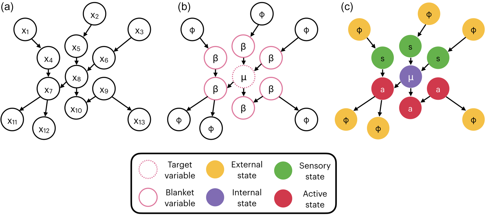
Figure 5. The Friston blanket. The three diagrams representing the stages of identifying a Friston blanket described in section 4.1. A system of interest is represented in the form a directed graph (a). Next the variable of interest is identified and a Markov blanket of shielding variables β is delineated separating the internal variable μ from the external ones denoted by ϕ (b). Finally, the variables within the blanket are identified as sensory s or active a depending on their relations with the external states (c).Footnote 9
Applied to the primordial soup simulation, each particle can be coloured to indicate which of these sets it has been assigned to (see Fig. 6). Given the dominance of short-range interactions and the density of particles, it should not come as a surprise that the particles that are labelled as active and sensory states form a spatial boundary around the states that are labelled as internal states. Given their placement in the simulated state space, one has the impression that the active and sensory states form a structure similar to a cell membrane.

Figure 6. The Markov blanket of the simulated soup at steady-state (adapted from Friston [Reference Friston2013] using the code provided). Similarly to Figure 3, particles are indicated by larger dots. Particles that belong to the set of sensory states are in green, active states are in red. Internal states are violet, while external states are marked in yellow. A “blanket” of active and sensory cells surrounding the internal particles can be seen.
The “Markov blanket formalism” advocated by Friston (Reference Friston2013) and described formally above does most of the work in the active inference literature when it comes to identifying internal, sensory, active, and external states. This formalizing step requires a number of non-trivial assumptions, some of which are now included in Friston et al., (Reference Friston, Da Costa and Parr2021a, Reference Friston, Fagerholm, Zarghami, Parr, Hipólito, Magrou and Razi2021b), but were not present in the original “Life as we know it” paper, and thus have been ignored in much of the subsequent literature. For example, it is unclear why only electrochemical interactions are used to construct the adjacency matrix while other forms of influence included in the simulation (such as Newtonian forces) are ignored. If different thresholds were used to determine whether two nodes are connected, the adjacency matrix would look very different. The demarcations made by analysing the adjacency matrix are then used to label the nodes in the original system (as in Fig. 6 above).
4.2 Friston blankets
The primordial soup simulation is claimed to provide a formal model for the emergence of agent–environment systems. We need to make a distinction between three different constructs: the “real” primordial soup (i.e., the target system), a model of the primordial soup (i.e., an idealized representation of the soup), and the adjacency matrix (i.e., a further abstraction of the idealized model). A Friston blanket, according to the treatment in Friston (Reference Friston2013), can be identified using the adjacency matrix once a set of nodes of interest has been identified.Footnote 10 A first interpretative step is taken when labelling the nodes of the idealized model as internal, external, active, and sensory states (i.e., as part of the Friston blanket). A further, and more problematic step is taken when extending the interpretation to the target system. The idea now is that, using the Markov blanket formalism, it is possible to uncover hidden properties of the target system that, in some sense, “instantiates” (Friston, Reference Friston2013, p. 2) or “possesses” (ibid. p. 1) a Markov blanket. This procedure of attributing a property of the map (the Bayesian network) to the territory (the simulated soup, and by implication, the real primordial soup itself) is problematic because it reifies abstract features of the map (cf. Andrews, Reference Andrews2020). A further implication of this step is that Markov blankets, which were initially introduced by Pearl as a formal property of directed, acyclical graphs, are now seen as real parts of systems explicitly modelled using non-directed connections between variables. This surprising shift has gone mostly unnoticed in the literature, even though no formal justification is provided.
There is ample evidence in the literature of this shift from model to target, which we might call a “reification fallacy.” For instance, Allen and Friston (Reference Allen and Friston2018) begin rather uncontroversially:
The boundary (e.g., between internal and external states of the system) can be described as a Markov blanket. The blanket separates external (hidden) from the internal states of an organism, where the blanket per se can be divided into sensory (caused by external) and active (caused by internal) states. (p. 2474)
It is possible to read this passage in an entirely instrumentalist way. That the boundary “can be described” using a blanket merely suggests that the system can be modelled as having a blanket (see for instance Friston, Reference Friston2013; Palacios, Razi, Parr, Kirchhoff, & Friston, Reference Palacios, Razi, Parr, Kirchhoff and Friston2020). Without considering the further assumptions explained in Biehl, Pollock, and Kanai (Reference Biehl, Pollock and Kanai2021) and Friston et al. (Reference Friston, Da Costa and Parr2021a), this notion of a Markov blanket is in line with the standard use of the notion introduced by Pearl and explained in the first part of this paper. However, Allen and Friston undermine this innocent instrumentalist reading on the very next page:
In short, the very existence of a system depends upon conserving its boundary, known technically as a Markov blanket, so that it remains distinguishable from its environment—into which it would otherwise dissipate. The computational ‘function’ of the organism is here fundamentally and inescapably bound up into the kind of living being the organism is, and the kinds of neighbourhoods it must inhabit. (p. 2475)
In this passage a Markov blanket is taken to be either equivalent to, or identical with, a physical boundary in the world.Footnote 11 Markov blankets here distinguish a system from its environment, much in the way a cell membrane does: the loss of a Markov blanket is equated with the loss of systemic integrity. This function is far removed from the initial auxiliary role played by Markov blankets in variational inference, where notions of temporal dynamics and system integrity do not come up. Instead, Markov blankets serve here as a real boundary between organism and world, that is, what we are calling a “Friston blanket.”
Many proponents of active inference now use the Markov blanket formalism in a much more metaphysically robust sense, one that does not simply follow from the formal details. Whereas the Pearl blankets discussed in the previous section are unambiguously part of the map (e.g., the graphical model), Friston blankets are best understood as parts of the territory (e.g., the system being studied). We will now look in more detail at some of the philosophical claims about agent–environment boundaries that Friston blankets have been taken to support.
4.3 Ambiguous boundaries
Why and how have Markov blankets been reified to act as parts of the target system, for example, by delineating its spatiotemporal boundaries, rather than merely being used as formal tools intended for scientific representation and statistical analysis? When did the map become conflated with the territory? Here we aim to answer this question by presenting a series of different treatments inspired by Friston's use of Markov blankets in “Life as we know it” (Reference Friston2013). In doing so we can see how what was once an abstract mathematical construct defined by conditional independences in graphical models (a Pearl blanket) came to be seen as an entity that somehow causes (or “induces,” or “renders”) conditional independence (a Friston blanket).Footnote 12 This latter interpretation has potentially interesting philosophical implications, but does not follow directly from the former mathematical construct. Perhaps surprisingly, many authors in the field are seemingly not aware of this process of reification, leading to the conflation of several different kinds of boundaries in the literature: Markov blankets are characterized alternatively as statistical boundaries, spatial boundaries, ontological boundaries, or autopoietic boundaries, and each characterization is treated as somehow equivalent to (and interchangeable with) the others.
Some authors are admittedly more careful, for example, Clark (Reference Clark, Metzinger and Wiese2017) makes sure to distinguish between the physical process (the territory) and the Bayesian network (the map):
Notice that the mere fact that some creature (a simple feed-forward robot, for example) is not engaging in active online prediction error minimization in no way renders the appeal to a Markov blanket unexplanatory with respect to that creature. The discovery of a Markov blanket indicates the presence of some kind of boundary responsible for those statistical independencies. The crucial thing to notice, however, is that those boundaries are often both malleable (over time) and multiple (at a given time), as we shall see. (p.4)
Here the discovery of a Markov blanket, perhaps only in our model of the system, serves to indicate the presence of “some kind of boundary” in the system itself. Clark holds that Markov blankets are discovered inside the modelling domain (what we call Pearl blankets), and that this discovery indicates the presence of something important (“some kind of boundary”) in the target domain (perhaps a Friston blanket). While relatively unobjectionable, this move seems to presuppose a tight (and hence non-arbitrary) relation between the model and its target domain of an agent and its environment, with potentially crucial consequences for our understanding of cognitive systems (cf. Clark's previous work on “cognitive extension” in e.g., Clark & Chalmers, Reference Clark and Chalmers1998).
In a similar fashion, other works reinforce the perspective that Markov blankets are a useful indicator to look for when attempting to define the boundaries of a system of interest. For example, Kirchhoff et al. (Reference Kirchhoff, Parr, Palacios, Friston and Kiverstein2018) write that:
A Markov blanket defines the boundaries of a system (e.g., a cell or a multi-cellular organism) in a statistical sense. (p. 1)
They also assume that this statement implies something much stronger, namely that
[A] teleological (Bayesian) interpretation of dynamical behaviour in terms of optimization allows us to think about any system that possesses a Markov blanket as some rudimentary (or possibly sophisticated) ‘agent’ that is optimizing something; namely, the evidence for its own existence. (p. 2)
However, the authors never explicate exactly how to conceive of a “boundary in a statistical sense,” perhaps indirectly relying on the inflated version of a Markov blanket proposed in Friston and Ao (Reference Friston and Ao2012) and Friston (Reference Friston2013).
Hohwy (Reference Hohwy, Metzinger and Wiese2017) also equates the internal states identified by a Markov blanket formalism with the agent:
The free energy agent maps onto the Markov blanket in the following way. The internal, blanketed states constitute the model. The children of the model are the active states that drive action through prediction error minimization in active inference, and the sensory states are the parents of the model, driving inference. If the system minimizes free energy — or the long-term average prediction error — then the hidden causes beyond the blanket are inferred. (pp. 3–4)
Furthermore, Hohwy assumes that the Markov blanket is not just a statistical boundary, but also an epistemic one. Because the external states are conditionally independent from the internal states (given the Markov blanket), the agent needs to infer the value of the external states (the “hidden causes”) based upon the information it is receiving “at” its Markov blanket, that is, the sensory surface. Hohwy even goes as far as to define the philosophical position of epistemic internalism in terms of a Markov blanket:
A better answer is provided by the notion of Markov blankets and self-evidencing through approximation to Bayesian inference. Here there is a principled distinction between the internal, known causes as they are inferred by the model and the external, hidden causes on the other side of the Markov blanket. This seems a clear way to define internalism as a view of the mind according to which perceptual and cognitive processing all happen within the internal model, or, equivalently, within the Markov blanket. This is then what non-internalist views must deny. (p. 7)
In other words, Markov blankets “epistemically seal-off” agents from their environment. In the same paper, Hohwy, like Allen and Friston above, equates an agent's physical boundary with the Markov blanket:
Crucially, self-evidencing means we can understand the formation of a well-evidenced model, in terms of the existence of its Markov blanket: if the Markov blanket breaks down, the model is destroyed (there literally ceases to be evidence for its existence), and the agent disappears. (p.4)
Finally, in a similar vein Ramstead et al. (Reference Ramstead, Badcock and Friston2018) characterize Markov blankets as at once statistical, epistemic, and systemic boundaries:
Markov blankets establish a conditional independence between internal and external states that renders the inside open to the outside, but only in a conditional sense (i.e., the internal states only ‘see’ the external states through the ‘veil’ of the Markov blanket; [32,42]). With these conditional independencies in place, we now have a well-defined (statistical) separation between the internal and external states of any system. A Markov blanket can be thought of as the surface of a cell, the states of our sensory epithelia, or carefully chosen nodes of the World Wide Web surrounding a particular province. (p. 4)
All of the above examples show how Markov blankets have moved from a rather simple statistical tool used for specifying a particular structure of conditional independence within a set of abstract random variables, to a specification of structures in the world that are said to “cause” conditional independence, separate an organism from its environment, or epistemically seal off agents from their environment.Footnote 13 These characterizations would sound bizarre to the average computer scientist and statistician familiar only with the original Pearl blanket formulation (perhaps the only people commonly aware of Markov blankets before 2012 or 2013). In the next section we will consider the novel construct of a Friston blanket in more detail, and highlight a number of additional assumptions that are necessary for Markov blankets to do the kind of philosophical work they have been proposed to do by the authors quoted above.
5. Conceptual issues with Friston blankets
So far, we have provided some initial analysis of both Pearl and Friston blankets, demonstrating that they are used to answer different kinds of scientific and philosophical questions. Since these are different formal constructs with different metaphysical implications, the scientific credibility of Pearl blankets should not automatically be extended to Friston blankets. In this section, we focus on two conceptual issues with Friston blankets. These conceptual issues illustrate the kinds of problems that arise when using conditional independence as a tool to settle the kinds of philosophical questions that we saw Friston blankets being applied to in the previous section.
To bring these conceptual issues into full view, let us introduce a second toy example. Consider how the conditions that lead up to and modulate the patellar reflex (or knee-jerk reaction) could be illustrated using a Bayesian graph. This is a common example of a mono-synaptic reflex arc in which a movement of the leg can be caused by mechanically stretching the quadriceps leg muscle by striking it with a small hammer. The stretch produces a sensory signal sent directly to motor neurons in the spinal cord, which, in turn, produce an efferent signal that triggers a contraction of the quadriceps femoris muscle (or what is observed more familiarly as a jerking leg movement). If we project these conditions onto a simple Bayesian network, we get something like Figure 7.

Figure 7. Conditions leading up to the knee-jerk reflex. On the left, a Bayesian network where i d and i p denote the motor intentions of the doctor and the patient respectively. Node s denotes the spinal neurons that are directly responsible for causing the kicking movement m. Node h indicates a medical intervention with a hammer, while c stands for a motor command sent to s from the central nervous system. Finally, node k stands for a third way of moving the patient's leg, for example, by someone else kicking it to move it mechanically. The middle (b) and the right figures (c) with the coloured-in nodes show two different ways of partitioning the same network using a “naive” Friston blanket with different choices of internal states, c and s respectively.
5.1 Counterintuitive sensorimotor boundaries
This simple network allows us to illustrate some problems with using Friston blankets to demarcate agents and their (sensorimotor) boundaries. The first problem concerns which role to attribute to co-parents in Friston blankets. Take s, that is, the activation of the cortical motor neurons, as the node of interest. As the graph makes clear, the activation of these neurons can be explained away by either a strike of a medical hammer into the tendon (h) or a motor command from the central nervous system (c).Footnote 14 This reflects the fact that the contraction of muscles isolated in the patellar reflex could also be the result of the patient's motor intentions. If we interpret the motor command c as an internal state of the patient, the spinal signal that causes the movement would be an active state. However, this leads to a puzzle about the way in which we should interpret h. Clearly, h is a co-parent of c and hence lies on its Friston blanket. According to the partition system used by Friston (Reference Friston2013, Reference Friston2019) and Friston et al. (Reference Friston, Fagerholm, Zarghami, Parr, Hipólito, Magrou and Razi2021b), h should fall into the Friston blanket of c as a sensory state (see Fig. 7b). But regardless of whether one assigns a sensory or active status to h, its inclusion in the Friston blanket of c is problematic. From a sensorimotor perspectiveFootnote 15 (see Barandiaran, Di Paolo, & Rohde, Reference Barandiaran, Di Paolo and Rohde2009; Tishby & Polani, Reference Tishby and Polani2011), h is an environmental variable external to the organism. As such, the medical hammer h should not be identified as part of an active agent, or even attributed a rather generous role as part of its sensory interface with the world.
One could object that our example delineates internal states in the wrong way, and that s should be considered an internal state, as in Figure 7c, while the bodily movement m and the external kick k should be considered, in the language of Friston blankets, as active states. Notice, however, that this would not help in any way, since what we might think of as an external intervention k that could lead to the same kind of bodily movement, is now part of the active states, while at the same time displaying the same formal properties as any putatively “internal” cause of the movement (as the Bayesian network in Fig. 7 should make clear). This example exposes the problem of differentiating between effects produced by an agent (internal states) and those brought about by nodes not constitutive of an agent (co-parents). The state of a node is not simply the joint product of its co-parents, as completely separate causal chains (the doctor's intention vs. the patient's intention) can produce the same outcome (i.e., spinal neuron activation). Hence the partitioning of the states into internal and external by means of a Markov blanket does not necessarily equate with the boundary between agent and environment found in sensorimotor loops, at least as these are intuitively or typically understood.
In other words, the co-parents of a child s in a Bayesian network include all other factors that could potentially cause, modulate, or influence the occurrence of s. This puts pressure on the analogy between Markov blankets and sensorimotor boundaries on which Friston blankets are based. Including these co-parents in the Friston blanket will include states in the environment (like the doctor's hammer), forcing one to accept counterintuitive conclusions about the boundaries of an agent. Not including the co-parents, on the other hand, gives up on the idea that conditional independence and Markov blankets are the right kind of tools to delineate the boundaries of agents, calling into question the validity of the Friston blanket construct as a formal tool.
5.2 Conditional independence is model-relative
A further, and perhaps even more substantial, problem is that conditional independence is itself model-relative. One possible objection to the patellar reflex network presented above is that the conditions making up the graph are not fine grained enough, that is, that the model is too simple. After all, the hammer does not directly intervene on the neurons in the spinal column, but rather on the tendon that causes the contraction of the muscle, which is responsible for the afferent signal that is the true proximal cause of the activation of the spinal motor neurons. However, just as it is difficult (and potentially ill-defined) to identify the most proximate cause of the knee-jerk, it is difficult to identify the most proximate cause and consequence of any internal state. Since the very distinction between sensory and active states (the sensorimotor boundary) and external states (the rest of the world) hangs upon the distinction between “most proximate cause” and “causes further removed,” the identifiability of such a cause is crucial.Footnote 16 This point is well made by Anderson (Reference Anderson, Wiese and Metzinger2017) who writes on the identifiability of the proximal cause:
An obvious candidate answer would be that I have access only to the last link in the causal chain; the links prior are increasingly distal. But I do not believe that identifying our access with the cause most proximal to the brain can be made to work, here, because I don't see a way to avoid the path that leads to our access being restricted to the chemicals at the nearest synapse, or the ions at the last gate. There is always a cause even “closer” to the brain than the world next to the retina or fingertip. (p. 4)
As has been mentioned in the previous section, Bayesian models are often explicitly said to be instrumental tools that are not designed to develop a final and complete description of a system, but are rather best at capturing the dependencies between the element of a system and/or predicting its behaviour, at a particular level of analysis (and relative to our current knowledge and resource constraints). What the “right” Bayesian network is for the knee-jerk reaction might depend on the observed states that we are given, our background knowledge and assumptions, and more pragmatically, the problem we want to model, as well as the time and computational power that is at our disposal. Which, and how many, Markov blankets can be identified within this model will depend on all of these factors. This suggests that Bayesian networks are not the right kind of tool to delineate real ontological boundaries in a non-arbitrary way. Here we are talking about Bayesian models in general, but an important caveat is that Bayesian networks have been famously used as tools for decomposing physical systems. Importantly, however, such decomposition relies on treating the model as a map of the target system, which is then used to direct interventions that can be modelled using Pearl's “do-calculus” (Pearl, Reference Pearl2009; cf. Woodward, Reference Woodward2003). Such applications of Bayesian modelling rarely make use of the Bayesian Occam's razor (mentioned in section 2.4.), since the goal is not to predict the behaviour of the system, but rather to depict how parts of the system influence each other.
What does this imply for the philosophical prospects of the Friston blanket construct serving as a sensorimotor boundary? Simply put, where Friston blankets are located in a model depends (at least partially) on modelling choices, that is, relevant Friston blankets cannot simply be “detected” in some objective way and then used to determine the boundary of a system.Footnote 17 This can be easily seen by the fact that Markov blankets are defined only in relation to a set of conditional (in)dependencies, or the equivalent graphical models (in either static systems, see Pearl [Reference Pearl1988], or dynamic regimes at steady-state, see Friston et al. [Reference Friston, Da Costa and Parr2021a]). The choice of a particular graphical model is then usually enforced by Bayesian model selection, which is in turn dependent on the data used (e.g., one cannot hope to model the firing activity of neurons, given as data fMRI recordings that already measure only at the grain of voxels). These considerations point, in our opinion, to a strongly instrumentalist understanding of Bayesian networks, and hence of Markov blankets, which would not justify the kinds of strong philosophical conclusions drawn by some from the idea of a Friston blanket (see e.g., cf. Andrews, Reference Andrews2020; Beni, Reference Beni2021; Friston et al., Reference Friston, Wiese and Hobson2020; Hohwy, Reference Hohwy2016; Sánchez-Cañizares, Reference Sánchez-Cañizares2021; Wiese & Friston, Reference Wiese and Friston2021 for some recent critical discussion).
While we do not want to try and solve all of these issues here, it is important to recognize that the notion of a Friston blanket as employed in the active inference literature is intended to carry out a very different role from the standard definition of a Pearl blanket used in the formal modelling literature. The open question here is whether Bayesian networks and Markov blankets are really the right kinds of conceptual tools to delineate the sensorimotor boundaries of agents and living organisms, or whether there are really two different kinds of project going on here, each of which deserves its own set of formal tools and assumptions. We turn to this question in the next section, but it is important to note that even if a legitimate explanatory project can be defined for Friston blankets, the conceptual issues outlined in this section will also still need to be addressed.
6. Two (very) different tools for two (very) different projects
So far, we have presented the conceptual journey on which Markov blankets have been taken. They started out as an auxiliary construct in the probabilistic inference literature (Pearl blankets), and have ended up as a tool for distinguishing agents from their environment (Friston blankets). The analysis above already showed the deep differences between Pearl blankets and Friston blankets, both in terms of their technical assumptions and of the general explanatory aims of these two constructs. However, in the literature on the FEP and active inference, the two have not yet really been distinguished. Even in very recent work there is an obvious conflation of Pearl and Friston blankets, using the former to define, justify, or explain the latter. For example, see the figures presented in Kirchhoff et al. (Reference Kirchhoff, Parr, Palacios, Friston and Kiverstein2018); Ramstead, Friston, and Hipólito (Reference Ramstead, Friston and Hipólito2020a); Sims (Reference Sims2020); and Hipólito et al. (Reference Hipólito, Ramstead, Convertino, Bhat, Friston and Parr2021), where Bayesian networks are used to describe what we would call Friston blankets. However, there are a series of extra assumptions that are necessary to move from Pearl blankets to Friston blankets, and these are rarely (if ever) explicitly stated or argued for. To give an initial example, Kirchhoff and Kiverstein (Reference Kirchhoff and Kiverstein2021) simply assume that the Markov blanket construct can be transposed from the formal to the physical domain, writing:
The notion of a Markov blanket is taken from the literature on causal Bayesian networks. Transposed to the realm of living systems, the Markov blanket allows for a statistical partitioning of internal states (e.g., neuronal states) from external states (e.g., environmental states) via a third set of states: active and sensory states. The Markov blanket formalism can be used to define a boundary for living systems that both segregates internal from external states and couples them through active and sensory states. (p. 2)
Such a transposition is not at all straightforward, and the phrasing “transposed to the realm of living systems” covers up a great explanatory leap from the merely formal Pearl blanket construct to the metaphysically laden Friston blanket, which is supposed to be instantiated by some physical system. The ambition of the philosophical prospects of the Friston blanket construct is again made clear by Kirchhoff and Kiverstein (Reference Kirchhoff and Kiverstein2021):
We employ the Markov blanket formalism to propose precise criteria for demarcating the boundaries of the mind that unlike other rival candidates for “marks of the cognitive” avoids begging the question in the extended mind debate. (p.1)
Based on what we have presented above however, the philosophical validity of using Friston blankets to draw the boundaries of the mind cannot simply be assumed from the formal credibility of the original Pearl blanket construct. We should emphasize at this point that it is not only Kirchhoff and Kiverstein (Reference Kirchhoff and Kiverstein2021) making this assumption, which is prevalent in much of the active inference literature that draws on Friston's (Reference Friston2013) “Life as we know it” paper discussed in section 4.1. In what follows we will consider the differences between the Pearl blanket and Friston blanket constructs in more detail, providing additional examples as we go.
6.1 Inference with a model and inference within a model
We are now in a position to articulate what we perceive to be the central methodological difference between how the two notions of Markov blankets are applied in the literature. As we see it, applications of the two constructs should be understood as representing different research programmes. The first, which we will call “inference with a model,” corresponds roughly to the use of Markov blankets (or Pearl blankets) described in section 3 of this paper. The main thesis that drives this research programme is that organisms perform variational inference to regulate perception and action. In doing so, they rely (implicitly or explicitly) on a model of their environment, which might feature something like Pearl blankets as an auxiliary statistical construct. The second research programme, which we call “inference within a model,” constitutes the position we described in section 4 of this paper, using Markov blankets (or Friston blankets) as a measure of the real ontological boundary between a system and its environment. The main thesis that drives this latter research programmes is that living systems and their environments are dynamically coupled systems that can be represented using network models, and that modelling tools (like Markov blankets) can therefore be legitimately used to distinguish an agent from its environment. These are two very different projects, with different commitments, aims, and tools (although both might fall broadly under the FEP framework). In the rest of this subsection we will briefly characterize both projects.
6.1.1 Inference with a model
As mentioned above, an important motivation for the FEP is the parallel between scientific inference and active inference. Like the scientist, the agent wants to know and control the states of some aspect of the world that remains hidden, while only having access to some limited set of observations. The agent can solve this problem by using a generative model of its environment. The agent uses (or appears to use) variational inference to obtain a recognition density that approximates the posterior density.
In model-based cognitive neuroscience, the two approaches have been stacked together. The explanatory project is to infer the details of the generative model an agent is using to infer the states of its environment. This seems to be one of the strongest potential empirical applications of the FEP and some of its related ideas (Adams, Stephan, Brown, Frith, & Friston, Reference Adams, Stephan, Brown, Frith and Friston2013; Parr et al., Reference Parr, Mirza, Cagnan and Friston2019; Pezzulo, Rigoli, & Friston, Reference Pezzulo, Rigoli and Friston2018), and reflects a more general explanatory strategy in cognitive neuroscience (Lee & Mumford, Reference Lee and Mumford2003; Rao & Ballard, Reference Rao and Ballard1999). Although perhaps not directly empirically refutable (cf. Andrews, Reference Andrews2020), this approach guides an active research programme, whose quality will eventually determine its overall viability.
As we highlighted in section 3.1, Pearl blankets play an auxiliary role in projects of this kind. They describe conditional independence on random variables (represented for instance in Bayesian networks), and are not a literal feature of either the agent or its environment (or indeed, the boundary between the two). There has been some discussion of the status of the theoretical posits of this kind of research. Do agents really possess a model of their environment, or are they merely usefully modelled as such? These questions about realism and instrumentalism of cognitive constructs are interesting and have been extensively discussed in the recent literature on active inference (Colombo & Seriès, Reference Colombo and Seriès2012; Ramstead, Kirchhoff, & Friston, Reference Ramstead, Kirchhoff and Friston2020b; Ramstead et al., Reference Ramstead, Friston and Hipólito2020a; van Es, Reference van Es2021), but these discussions are not our main focus. The framing of the agent as a modeller of its environment has also led to an important but rather long-winded debate about whether, and in what sense, free energy minimizing agents should be seen as utilizing generative models as representations of their environment (Clark, Reference Clark2015a, Reference Clark2015b; Dołęga, Reference Dołęga, T. K. Metzinger and W. Wiese2017; Gładziejewski, Reference Gładziejewski2016; Kiefer & Hohwy, Reference Kiefer and Hohwy2018; Kirchhoff & Robertson, Reference Kirchhoff and Robertson2018; Williams, Reference Williams2018). Here we merely point out that this debate also allows for taking an instrumentalist or realist stance and, more importantly, that it is orthogonal to the distinction between inference with a model and inference within a model.
One complicating factor that is worth mentioning here is a potential disanalogy between scientific inference and active inference. In scientific inference, a scientist literally uses a model to make inferences out of observed data. The model itself is inert when not being used by an intentional agent. The same does not go for active inference. The agent does not have a model of its environment that it uses to perform inference, but rather the agent is a model of its environment (Baltieri & Buckley, Reference Baltieri and Buckley2019; Bruineberg, Kiverstein, & Rietveld, Reference Bruineberg, Kiverstein and Rietveld2018; Friston, Reference Friston2013; Friston, Reference Friston2019). There is no separate entity that uses a generative model to perform inference, instead the agent performs (or appears to perform) inference, and it is at once both scientist and model. Considerations of this kind have led some theorists to turn towards a different (and perhaps more ambitious) explanatory project, where Markov blankets also come to be seen as a literal part of the physical systems being studied.
6.1.2 Inference within a model
The “primordial soup simulation” that we presented in section 4.2 suggests a very different research direction for the active inference framework. This simulation starts out with a soup of coupled particles and aims to show how a distinction between “agent” and “environment” emerges as the dynamics of the system reach equilibrium. Agent and environment are separated by each other through a Friston blanket. The Markov blanket formalism has subsequently been presented as not just being able to identify the boundaries of agents, but also of any supposedly self-organizing system, including species (Ramstead et al., Reference Ramstead, Kirchhoff, Constant and Friston2019) and biospheres (Rubin et al., Reference Rubin, Parr, Da Costa and Friston2020).
One could see the primordial soup simulation as an interesting toy model to investigate the emergence of sensorimotor boundaries in a highly idealized domain. This has long been a successful strategy in complex systems research. For example, Conway's Game of Life (Gardner, Reference Gardner1970) has been used to formalize concepts such as autopoiesis (Beer, Reference Beer2004, Reference Beer2014, Reference Beer2020). Such toy models come with strong explanatory power but also forthright metaphysical modesty: they do not claim to directly model or capture real-world phenomena. They are merely used as demonstrations of how certain concepts or principles could play out in a simplified system. This, however, is very different from how most active inference theorists frame their work, as we will now see.
Perhaps the clearest expression of the metaphysical commitments implied by the use of Friston blankets is provided by Ramstead et al. (Reference Ramstead, Kirchhoff, Constant and Friston2019), who write:
The claims we are making about the boundaries of cognitive systems are ontological. We are using a mathematical formalism to answer questions that are traditionally those of the discipline of ontology, but crucially, we are not deciding any of the ontological questions in an a priori manner. The Markov blankets are a result of the system's dynamics. In a sense, we are letting the biological systems carve out their own boundaries in applying this formalism. Hence, we are endorsing a dynamic and self-organising ontology of systemic boundaries. (p. 3)
The claim seems to be that the answers to these ontological questions can be simply assumed by doing the maths and then checking where the Markov blanket lies. In order for the formalism to do such heavy metaphysical lifting, however, additional premises need to be in place. After all, cognitive systems (or other systems whose boundaries we might be interested in) exist in the physical world, while the original Markov blanket formalism operates on abstract mathematical entities. Hence, the question for proponents of the more ambitious FEP project is: how can the two kinds of entities map onto each other, such that conclusions about the boundaries of cognitive systems can be drawn based on the mathematical framework?
As we have hinted at before, there are three strategies available to the FEP theorist who wants to use Markov blankets in this way: a literalist, realist, and an instrumentalist one. The literalist position is roughly equivalent to the claim that the world just is a network consisting of interacting systems, which are themselves more fine-grained probabilistic networks, and so on, and this is why the Friston blanket formalism works as a way to demarcate real-world boundaries. The realist position is still committed to the claim that Friston blankets do pick out real boundaries in the world, but they are taken to be representations of worldly features, rather than literally being such features themselves. Finally, the instrumentalist position holds that the world can merely be usefully modelled as a Bayesian network, and that this justifies using the Pearl blanket formalism as a guide to worldly boundaries. We think that both the literalist and realist positions have similar problems, while the instrumentalist position is less problematic but also less interesting. We will discuss each position in turn.
The literalist position entails that the mathematical structures posited by the FEP are not merely a map of self-organizing systems, but are themselves the territory (cf. Andrews, Reference Andrews2020). In this case, the FEP framework might constitute something like a “blanket-oriented ontology” (BOO): a view in which reality consists of a number of hierarchically nested Friston blankets. This might be an appealing picture for some, but it is certainly not something that can be simply read off the formalism itself. Rather, it is an additional assumption that must be explicitly stated and argued for. In a recent paper, Menary and Gillett (Reference Menary, Gillett, Mendonca, Curado and Gouveia2020) point out the strong Platonist and Pythagorean attitude that would be necessary in order to motivate this kind of ontology. Such an approach is not without allure and could be made philosophically interesting, but it would certainly not be metaphysically agnostic. The FEP and Friston blankets would serve as a starting assumption of such an ontological project, rather than its end goal. At any rate, the resulting approach would be quite far removed from the empirical and naturalistic research programme that FEP purports to be, and would certainly involve answering “ontological questions in an a priori manner” (Ramstead et al., Reference Ramstead, Kirchhoff, Constant and Friston2019, p. 3).
At first sight, the realist alternative might look less objectionable. Conclusions can be drawn about real-world systems because there is a systematic mapping between reality and our mathematical descriptions of reality in terms of Bayesian networks. After all, it is relatively easy to find some mapping between a given target and the assumed model domain. However, the difficulty lies in finding a non-arbitrary mapping that is privileged for principled reasons. In the literature on Bayesian inference, the gold standard for establishing what the right kind of model is for a given target domain is Bayesian model selection. This requires a set of observations that is then used to select the most parsimonious explanatory model of these observations (see sect. 2.4). In turn, Friston blankets can be understood only relative to such a model (see sect. 5.2). The puzzle then is that if one wants to use the Markov blanket formalism to demarcate the boundaries of, for example, a cognitive agent, one needs to already have a principled justification for why to start from one particular model rather than a different one, at which point it is not clear that the Markov blanket formalism is doing much additional work.
Some authors have followed this path and advocated for the realist position by claiming that it is not the Markov blanket alone, but rather the Markov blanket plus the FEP, that provides the relevant demarcations of agent–environment boundaries. Only those Markov blankets that demarcate free energy minimizing systems (or the systems that minimize the most free energy, see Hohwy, Reference Hohwy2016) can be taken to represent the boundaries of living or cognitive systems. This defense of Friston blankets might look appealing at first, but faces a serious obstacle by assuming that free energy minimizing systems can be identified without the help of the assumptions behind the Friston blanket construct, such as the existence of unambiguously active or passive states. This is a problem because, as it turns out, it is not that difficult to characterize all sorts of systems as free energy minimizing systems. For example, Baltieri, Buckley, and Bruineberg (Reference Baltieri, Buckley and Bruineberg2020) show that even the humble Watt governor can be analysed as a free energy minimizing system. Elsewhere, Rubin et al. (Reference Rubin, Parr, Da Costa and Friston2020) have proposed modelling the Earth's climate system as the planet's own Friston blanket, while Parr (Reference Parr2021) uses Friston blankets to model enzymatic reactions in biochemical networks. What these examples show is that the scope of the free energy formula is so broad that it is inadequate to pick out only living or cognitive systems. One could bite the bullet and claim that planets and Watt governors are cognitive systems, but this would be a surprising result and few would be on board with such radical assumptions. Finally, as we saw in section 2, the FEP already assumes a mathematical structure to be in place (be it a random dynamical system or a Bayesian network). Therefore, in and of itself, the FEP has nothing to say about how these mathematical structures should be mapped onto physical structures.
All of the above suggest that Bayesian networks are not the right kind of tools to delineate real-world boundaries in an objective and non-question-begging way. Perhaps ultimately these problems are resolvable, but as far as we know, nearly no-one in the literature has thus far paid any attention to them (for a refreshing exception see Biehl [Reference Biehl2017], and some of the references therein). These considerations have led some authors behind the more recent active inference literature to embrace instrumentalism about the whole framework, not just the Friston blanket construct. Some have suggested that the active inference framework should subscribe to a fundamentally instrumentalist approach to scientific investigation, such that the use of Markov blankets to demarcate organism–environment boundaries should be understood just as another feature of our (scientific) models, rather than making any ontological claims about the structure of the world (see e.g., Andrews, Reference Andrews2020; Colombo, Elkin, & Hartmann, Reference Colombo, Elkin and Hartmann2018; Ramstead et al., Reference Ramstead, Friston and Hipólito2020a, Reference Ramstead, Kirchhoff and Friston2020b; van Es, Reference van Es2021). This kind of global scientific instrumentalism is fine so far as it goes, and of course has precedents elsewhere in the philosophical debates about scientific realism (see e.g., Chakravartty, Reference Chakravartty and Zalta2017 for a helpful overview), but we do not think that it is reflective of the attitude that most scientists (or even philosophers) take towards the kinds of claims being made about Friston blankets in the active inference literature. Such global instrumentalism definitely does not sit well with the BOO described above, and seems to be incompatible with understanding FEP as providing a “formal ontology” (Ramstead et al., Reference Ramstead, Kirchhoff, Constant and Friston2019). Nonetheless, we are happy to settle for a conditional conclusion here: insofar as one is a scientific realist, and treats the seemingly ontological claims made about Friston blankets in a realist manner, then some further metaphysical assumptions are needed in order to warrant these claims.
7. Conclusion
Despite all of the issues and ambiguities pointed out in our above treatment, the FEP and active inference framework have considerable following in the fields of neuroscience and biology, due in part to ambitious claims regarding their unificatory potential (Friston, Reference Friston2010, Reference Friston2019; Friston et al., Reference Friston, FitzGerald, Rigoli, Schwartenbeck and Pezzulo2017a; Hesp et al., Reference Hesp, Ramstead, Constant, Badcock, Kirchhoff and Friston2019; Kuchling, Friston, Georgiev, & Levin, Reference Kuchling, Friston, Georgiev and Levin2020). Under the umbrella term of predictive processing, they have also gained popularity in philosophy of mind and cognitive science, where they appear to play the role of a new conceptual tool that could settle centuries-long disputes about the relationship between mind and life (Clark, Reference Clark2013, Reference Clark2015a, Reference Clark2020; Friston et al., Reference Friston, Wiese and Hobson2020; Hohwy, Reference Hohwy2013). At the same time, different parts of the framework have raised some important, and in some cases yet-to-be-answered, scientific and philosophical problems. Some of these problems have to do with the capacity of the framework to account for traditional folk psychological distinctions between belief and desire (see e.g., Dewhurst, Reference Dewhurst2017; Klein, Reference Klein2018; Yon, Heyes, & Press, Reference Yon, Heyes and Press2020), although its defenders have argued that it can account for desire in a novel way (Clark, Reference Clark2020; Wilkinson, Deane, Nave, & Clark, Reference Wilkinson, Deane, Nave and Clark2019). Another, very common, kind of critique is that the framework either does not enjoy any empirical support, or that the FEP is empirically inadequate (Colombo & Palacios, Reference Colombo and Palacios2021; Colombo & Wright, Reference Colombo and Wright2021; Williams, Reference Williams2021), and should therefore be considered to offer, at best, a redescription of existing data (see e.g., Cao, Reference Cao2020; Colombo et al., Reference Colombo, Elkin and Hartmann2018; Liwtin & Miłkowski, Reference Litwin and Miłkowski2020). Yet another kind of critique argues that there is no significant connection between the (a priori) FEP formalism on the one hand, and the (empirical) process theories it is intended to support on the other (Colombo & Palacios, Reference Colombo and Palacios2021; Colombo & Wright, Reference Colombo and Wright2021; Williams, Reference Williams2021), or that it presents a false equivocation between probability and adaptive value (Colombo, Reference Colombo2020). Other works, such as Di Paolo, Thompson, and Beer (Reference Di Paolo, Thompson and Beer2021) and Raja, Valluri, Baggs, Chemero, and Anderson (Reference Raja, Valluri, Baggs, Chemero and Anderson2021) have recently disputed claims about the FEP representing a general unifying principle, claiming that it fails to account for different sensorimotor aspects of embodied and (autopoietic) enactive cognition.
More relevant for what we have discussed here, Andrews (Reference Andrews2020) and van Es (Reference van Es2021) have recently argued against a realist interpretation of the mathematical models described by FEP, which are claimed to be better interpreted instrumentally. Along the same lines, Baltieri et al. (Reference Baltieri, Buckley and Bruineberg2020) provided a worked-out example of this instrumentalist view, where an engine coupled to a Watt (centrifugal) governor is shown to perform active inference as an example of “pan-(active-)inferentionalism,” asking what can possibly be gained by thinking of the behaviour of a coupled engine-mechanical governor system in terms of perception-action loops under the banner of free energy minimization. Finally, various technical aspects of the FEP are now under scrutiny in works such as Rosas, Mediano, Biehl, Chandaria, and Polani (Reference Rosas, Mediano, Biehl, Chandaria, Polani, Verbelen, Lanillos, Buckley and De Boom2020); Biehl et al. (Reference Biehl, Pollock and Kanai2021); and Aguilera, Millidge, Tschantz, and Buckley (Reference Aguilera, Millidge, Tschantz and Buckley2021). Rosas et al. (Reference Rosas, Mediano, Biehl, Chandaria, Polani, Verbelen, Lanillos, Buckley and De Boom2020) define a new object, a “causal blanket,” based on ideas from computational mechanics, in an attempt to overcome assumptions about Langevin dynamics in a stationary/steady-state regime. Biehl et al. (Reference Biehl, Pollock and Kanai2021) cast doubts on the inconsistent mathematical treatment of Markov blankets over the years, partially acknowledged by Friston et al. (Reference Friston, Da Costa and Parr2021a) who now address such differences and specifies new and more detailed constraints for a cohesive treatment of Markov blankets in the FEP (see endnote 9). Aguilera et al. (Reference Aguilera, Millidge, Tschantz and Buckley2021), on the other hand, question the relevance of the FEP for sensorimotor accounts of living systems, given some of its assumptions and in particular the description of agents' behaviour in terms of free energy gradients on ensemble averages of trajectories, claiming that (under the mathematical assumptions presented in their paper) these “free energy gradients [are] uninformative about the behaviour of an agent or its specific trajectories” (see also Di Paolo et al. [Reference Di Paolo, Thompson and Beer2021] for a similar conceptual point, and Da Costa, Friston, Heins, & Pavliotis [Reference Da Costa, Friston, Heins and Pavliotis2021] and Parr, Da Costa, Heins, Ramstead, & Friston [Reference Parr, Da Costa, Heins, Ramstead and Friston2021] for possible counterarguments).
These latter works come closest, at least in spirit, to the topics discussed in this paper, which have to do with a disconnect between the formal properties of Markov blankets and the way they are deployed to support metaphysical claims made by the FEP, especially in the context of active agents and living organisms. After having been initially developed in the context of (variational) inference problems, as a tool to simplify the calculations of approximate posteriors by taking advantage of relations of conditional independence (Bishop, Reference Bishop2006; Murphy, Reference Murphy2012), Markov blankets have been claimed by proponents of the FEP to clarify the boundaries of the mind (Clark, Reference Clark, Metzinger and Wiese2017; Hohwy, Reference Hohwy, Metzinger and Wiese2017; Kirchhoff & Kiverstein, Reference Kirchhoff and Kiverstein2021), of living systems (Friston, Reference Friston2013; Kirchhoff, Reference Kirchhoff2018; Kirchhoff et al., Reference Kirchhoff, Parr, Palacios, Friston and Kiverstein2018), and even of social systems (Fox, Reference Fox2021; Ramstead et al., Reference Ramstead, Badcock and Friston2018; Rubin et al., Reference Rubin, Parr, Da Costa and Friston2020; Veissière et al., Reference Veissière, Constant, Ramstead, Friston and Kirmayer2020). Interestingly, in these papers a system gets defined in terms of relations of independence made within a Bayesian network. In other words, the Bayesian network takes precedence over the physical world that it is supposed to model. In some passages it even appears that the world itself is taken to be a Bayesian network, with the Markov blankets defining what it is to be a “thing” within this world (Friston, Reference Friston2013; Friston, Reference Friston2019; Hipólito et al., Reference Hipólito, Ramstead, Convertino, Bhat, Friston and Parr2021; Kirchhoff et al., Reference Kirchhoff, Parr, Palacios, Friston and Kiverstein2018). We then raised some possible issues with this approach, namely the question of whether Bayesian networks are merely an instrumental modelling tool for the FEP framework, or whether the framework presupposes some kind of more fundamental Bayesian graphical ontology.
All of this points towards a fundamental dilemma for anyone interested in using Markov blankets to make substantial philosophical claims about biological and cognitive systems (which is what we take proponents of the FEP to be wanting to do). On the one hand, Markov blankets can be used in their original Pearl blanket guise, as a formal mathematical construct for performing inference on a generative model. This usage is philosophically innocent but cannot, without further assumptions that need to be explicitly stated, justify the kinds of conclusions that it is sometimes used for in the FEP literature (see e.g., Hohwy, Reference Hohwy, Metzinger and Wiese2017; Kirchhoff et al., Reference Kirchhoff, Parr, Palacios, Friston and Kiverstein2018; Kirchhoff & Kiverstein, Reference Kirchhoff and Kiverstein2021). On the other hand, Markov blankets can be used in a more ontologically robust fashion, as what we have called Friston blankets, to demarcate actual worldly boundaries. This is surely a more exciting application of the Markov blanket formalism, but it cannot be simply or innocently read off the mathematics of the more standard usage advocated in statistics and machine learning (Pearl, Reference Pearl1988), and requires some additional technical (Biehl et al., Reference Biehl, Pollock and Kanai2021; Friston, Reference Friston2019; Parr, Da Costa, & Friston, Reference Parr, Da Costa and Friston2020) and philosophical (Friston et al., Reference Friston, Wiese and Hobson2020; Hipólito et al., Reference Hipólito, Ramstead, Convertino, Bhat, Friston and Parr2021; Ramstead et al., Reference Ramstead, Badcock and Friston2018) assumptions that may in the end be doing all of the interesting work themselves.
The difference between inference with and inference within a model, here roughly corresponding to the use of Pearl and Friston blankets, shows why the potential payoff of the latter construct is much larger than the former. In inference with a model, the graphical model is an epistemic tool for a scientist or organism to perform inference. In inference within a model the scientist disappears from the scene, becoming a mere spectator of the inference show unfolding before their eyes. Here the Friston blanket specifies the anatomy of the target system: it is a formalization of the boundary between this system and its environment.
Ultimately, the considerations presented in this paper leaves the FEP theorist with a choice. One can accept a rather technical and innocent conception of Markov blankets as an auxiliary formal concept that define what nodes are relevant for variational inference. This conception is admittedly scientifically useful but has not yet lead to any philosophically interesting conclusions about the nature of life or cognition. Alternatively, one can import a number of stronger metaphysical assumptions about the mathematical structure of reality to support a realist reading, where the blanket becomes a literal boundary between agents and their environment. Such a strong realist reading cannot be justified by just “doing the maths,” but rather needs to be independently argued for, and no such argument has yet been offered.
Acknowledgments
The authors would like to thank Micah Allen, Mel Andrews, Martin Biehl, Daniel Dennett, Kevin Flowers, Hajo Greif, Julian Kiverstein, Richard Menary, Thomas Parr, Nina Poth, Maxwell Ramstead, Fernando Rosas, Matthew Sims, Filippo Torresan, Wanja Wiese, Tobias Schlicht and members of his research group, Marcin Miłkowski and members of his research group, and the Active Inference Lab for insightful and critical discussions and timely feedback on previous versions of the manuscript. The authors also thank the editor and eight reviewers for their time and effort. The manuscript has benefited enormously from their critical reports.
Financial Support
JB is funded by a Macquarie Research Fellowship. KD's work is funded by the Volkswagen Stiftung grant no. 87 105. MB is a JSPS International Research Fellow supported by a KAKENHI Grant-in-Aid for Scientific Research (No. JP19F19809).
Conflict of Interest
None.


Target article
The Emperor's New Markov Blankets
Related commentaries (35)
A continuity of Markov blanket interpretations under the free-energy principle
Against free energy, for direct perception
Bayesian realism and structural representation
Blankets, heat, and why free energy has not illuminated the workings of the brain
Boundaries and borders gone! But life goes on
Causal surgery under a Markov blanket
Does the metaphysical dog wag its formal tail? The free-energy principle and philosophical debates about life, mind, and matter
Embracing sensorimotor history: Time-synchronous and time-unrolled Markov blankets in the free-energy principle
Enough blanket metaphysics, time for data-driven heuristics
Free-energy pragmatics: Markov blankets don't prescribe objective ontology, and that's okay
Good theoretical debate, but insufficient proof of concept
Life, mind, agency: Why Markov blankets fail the test of evolution
Making life and mind as clear as possible, but not clearer
Making reification concrete: A response to Bruineberg et al.
Maps and territories, smoke, and mirrors
Markov blankets and Bayesian territories
Markov blankets and the preformationist assumption
Markov blankets as boundary conditions: Sweeping dirt under the rug still cleans the house
Markov blankets do not demarcate the boundaries of the mind
Markov blankets: Realism and our ontological commitments
Nothing but a useful tool? (F)utility and the free-energy principle
Practical implications from distinguishing between Pearl blankets and Friston blankets
Recurrent, nonequilibrium systems and the Markov blanket assumption
Redressing the emperor in causal clothing
Return of the math: Markov blankets, dynamical systems theory, and the bounds of mind
Scientific realism about Friston blankets without literalism
Spatiotemporal constraints of causality: Blanket closure emerges from localized interactions between temporally separable subsystems
The emperor has no blanket!
The empire strikes back: Some responses to Bruineberg and colleagues
The map, the territory, and the cartographer: Linking the “pure” formal models to the “murky” material world
The seductive allure of cargo cult computationalism
There is no “inference within a model”
What realism about agents requires
What's special about space?
Who tailors the blanket?
Author response
The Emperor Is Naked: Replies to commentaries on the target article