


1 Introduction
A long-standing problem in vortex dynamics is the construction of equilibrium vortex shapes. Given the complexity of the problem, the two-dimensional case has been the subject of particular attention, given its relevance to situations with weak variations in one direction, for example because of stratification. The two-dimensional flow due to a point vortex in an otherwise irrotational flow is described by the complex potential
 $$\begin{eqnarray}w=\unicode[STIX]{x1D719}+\text{i}\unicode[STIX]{x1D713}=\frac{\unicode[STIX]{x1D6E4}}{2\unicode[STIX]{x03C0}\text{i}}\ln z,\end{eqnarray}$$
where
 $\unicode[STIX]{x1D6E4}$
is the circulation of the vortex and
$\unicode[STIX]{x1D6E4}$
is the circulation of the vortex and
 $z=x+\text{i}y$
. While the point vortex is a useful model for the behaviour of the fluid outside the vortex (where the distance from the vortex is much larger than the core size), it is less useful for modelling the behaviour and dynamics of the vortex core and the motion of the fluid close to the vortex. This has motivated research into desingularizations of the point vortex, in particular using vortex sheets and vortex patches.
$z=x+\text{i}y$
. While the point vortex is a useful model for the behaviour of the fluid outside the vortex (where the distance from the vortex is much larger than the core size), it is less useful for modelling the behaviour and dynamics of the vortex core and the motion of the fluid close to the vortex. This has motivated research into desingularizations of the point vortex, in particular using vortex sheets and vortex patches.
A vortex sheet is a discontinuity in the velocity of the fluid, and the strength of the sheet is related to the jump in velocity tangential to the sheet as one crosses from one side to the other. This configuration is a delta function of vorticity in the direction normal to the sheet. A closed vortex sheet is one possible desingularization of a point vortex. It can also be viewed as a bubble with circulation. Far from the vortex sheet, the flow resembles that due to a point vortex as in (1.1).
Previous work on equilibrium vortex sheets has focused on hollow vortices, for which the density vanishes inside the vortex. Studies of hollow vortices examined equilibrium solutions such as pairs (Pocklington Reference Pocklington1895; Moore & Pullin Reference Moore and Pullin1987; Leppington Reference Leppington2006) or rows (Baker, Saffman & Sheffield Reference Baker, Saffman and Sheffield1976; Ardalan, Meiron & Pullin Reference Ardalan, Meiron and Pullin1995). More recently, Llewellyn Smith & Crowdy (Reference Llewellyn Smith and Crowdy2012) investigated both the shape and stability of a single steady hollow vortex in a straining field, and gave a description of its stability. Other work has looked at the von Kármán street of hollow vortices (Crowdy & Green Reference Crowdy and Green2011) and at hollow vortices in a channel (Green Reference Green2015).
A vortex patch is an area of fluid containing non-zero vorticity. As with the vortex sheet, far from the patch, the flow looks like the flow due to a point vortex with the same circulation. Here, we focus only on patches of uniform vorticity. In this case, the problem can be reduced from the underlying partial differential equations to contour dynamics (Zabusky, Hughes & Roberts Reference Zabusky, Hughes and Roberts1979), which requires only knowledge of the boundary of the vortex patches. This method was also used to calculate new vortex patch configurations termed V-states. Deem & Zabusky (Reference Deem and Zabusky1978) used this method to find new rotating and translating states of vortex patches, besides the known Kirchhoff vortices (Lamb Reference Lamb1932). It was used for both individual vortex patches and to look at the interactions between multiple vortex patches.
Moore & Saffman (Reference Moore, Saffman, Olsen, Goldburg and Rogers1971) calculated steady elliptical states of a vortex patch in a straining field. This work also included a stability analysis that found those ellipses that were neutrally stable and could be the starting states for bifurcated solutions of different shapes. Kamm (Reference Kamm1987) used Schwarz functions to investigate non-elliptical vortex patches in strain. The bifurcation points of the family of elliptical solutions matched those predicted by Moore & Saffman (Reference Moore, Saffman, Olsen, Goldburg and Rogers1971), and all the non-elliptical vortices in strain were found to be unstable. The three-dimensional stability was investigated in Robinson & Saffman (Reference Robinson and Saffman1984) and Miyazaki, Imai & Fukumoto (Reference Miyazaki, Imai and Fukumoto1995). Kida (Reference Kida1981) obtained solutions for vortex patches in uniform shear.
The Sadovskii vortex is a combination of the previously discussed vortex desingularizations: it is a vortex patch surrounded by a vortex sheet. (Such flows have been called ‘Batchelor flows’ in the literature, but we avoid the expression ‘Batchelor vortex’ to minimize confusion with the Batchelor vortex, which refers to a three-dimensional vortex with axial flow.) This type of flow was previously investigated in works on bluff-body wakes, including in Chernyshenko (Reference Chernyshenko1998). The Prandtl–Batchelor theorem shows that the vorticity inside a closed streamline tends to a constant value in the high-Reynolds-number limit (Batchelor Reference Batchelor1956a ). Batchelor (Reference Batchelor1956b ) argued that, in bluff-body wakes, the region of constant vorticity is bounded by a jump in tangential velocity (a vortex sheet), motivating further work, including that of Sadovskii (Reference Sadovskii1971), who investigated a flow in which there is a jump in the Bernoulli constant on the boundary of the vortex and the vorticity is organized into two patches of equal and opposite vorticity. Outside this region, the flow is incompressible and irrotational.
Other related works are Saffman & Tanveer (Reference Saffman and Tanveer1984) and Moore, Saffman & Tanveer (Reference Moore, Saffman and Tanveer1988). The latter obtained the Prandtl–Batchelor flow past a body with a forward-facing flap. This leads to an area of constant vorticity inside this angled section, and irrotational flow outside a streamline going from one edge of the plate to the other, which is a vortex sheet, as manifested by a jump in the Bernoulli constant. This problem was solved using conformal mappings for the inside and outside of the vortex, and then finding the correspondence between the boundary points in each mapping. Bunyakin, Chernyshenko & Stepanov (Reference Bunyakin, Chernyshenko and Stepanov1996, Reference Bunyakin, Chernyshenko and Stepanov1998) and Chernyshenko et al. (Reference Chernyshenko, Galletti, Iollo and Zannetti2003) investigated flows with vortex patches trapped in airfoil cavities.
Our goal here is to generalize the hollow vortex in strain of Llewellyn Smith & Crowdy (Reference Llewellyn Smith and Crowdy2012) and the elliptical vortex patches in strain of Moore & Saffman (Reference Moore, Saffman, Olsen, Goldburg and Rogers1971) by computing the Sadovskii vortex in strain. There will now be two governing non-dimensional parameters and the solutions will form a manifold in this parameter space. The relation between the known solutions is particularly interesting, because the Moore–Saffman vortices have a known bifurcation structure, while no such structure exists for the hollow vortex in strain. The case of a vortex in strain is a canonical one, since locally any flow looks like a strain, so this flow gives the local response of a vortex in a large-scale and more general complicated flow.
This paper is structured as follows. Section 2 describes the problem and boundary conditions. Sections 3 and 4 use numerical continuation to recalculate solutions to the patch and sheet cases, including families of bifurcating solutions. Section 5 presents solutions to the Sadovskii vortex in strain, and discusses the changes in the bifurcation diagram and vortex shapes as the contributions from interior and boundary circulation change. Section 6 presents conclusions. A discussion of the numerical method is given in the Appendix.
2 Formulation
The Sadovskii vortex is a patch of fluid with uniform vorticity surrounded by a vortex sheet. Inside the vortex, we require constant vorticity
 $\unicode[STIX]{x1D714}$
, so we solve Poisson’s equation
$\unicode[STIX]{x1D714}$
, so we solve Poisson’s equation
 $$\begin{eqnarray}\unicode[STIX]{x1D6FB}^{2}\unicode[STIX]{x1D713}=-\unicode[STIX]{x1D714},\end{eqnarray}$$
where
 $\unicode[STIX]{x1D713}$
is the streamfunction with
$\unicode[STIX]{x1D713}$
is the streamfunction with
 $$\begin{eqnarray}u=\frac{\unicode[STIX]{x2202}\unicode[STIX]{x1D713}}{\unicode[STIX]{x2202}y},\quad v=-\frac{\unicode[STIX]{x2202}\unicode[STIX]{x1D713}}{\unicode[STIX]{x2202}x}.\end{eqnarray}$$
Outside the vortex, the flow is irrotational, so we solve Laplace’s equation
 $$\begin{eqnarray}\unicode[STIX]{x1D6FB}^{2}\unicode[STIX]{x1D713}=0.\end{eqnarray}$$
We require that, far from the vortex, the streamfunction corresponds to a straining field along with circulation, so that
 $$\begin{eqnarray}\unicode[STIX]{x1D713}\sim \unicode[STIX]{x1D6FE}(x^{2}-y^{2})-\frac{\unicode[STIX]{x1D6E4}}{2\unicode[STIX]{x03C0}}\ln |z|\quad \text{as }|z|\rightarrow \infty ,\end{eqnarray}$$
where
 $\unicode[STIX]{x1D6FE}$
gives the strength of the strain.
$\unicode[STIX]{x1D6FE}$
gives the strength of the strain.
We require the boundary of the vortex to be a streamline, which means that
 $$\begin{eqnarray}\unicode[STIX]{x1D713}=\text{const.}\end{eqnarray}$$
on the boundary of the vortex. Since we can define the streamfunction
 $\unicode[STIX]{x1D713}$
up to a constant, without loss of generality we set
$\unicode[STIX]{x1D713}$
up to a constant, without loss of generality we set
 $\unicode[STIX]{x1D713}=0$
on the boundary. This condition can also be written in terms of the velocity as
$\unicode[STIX]{x1D713}=0$
on the boundary. This condition can also be written in terms of the velocity as
 $$\begin{eqnarray}\boldsymbol{u}\boldsymbol{\cdot }\hat{\boldsymbol{n}}=0,\end{eqnarray}$$
where
 $\boldsymbol{u}=(u,v)$
is the velocity and
$\boldsymbol{u}=(u,v)$
is the velocity and
 $\hat{\boldsymbol{n}}$
is the normal vector to the vortex boundary.
$\hat{\boldsymbol{n}}$
is the normal vector to the vortex boundary.
The second condition is the dynamic condition, which we also call the pressure condition or Bernoulli condition. As in Saffman (Reference Saffman1992), the Bernoulli condition for steady inviscid incompressible flows in regions with constant vorticity and no body forces is
 $$\begin{eqnarray}\frac{\unicode[STIX]{x1D70C}}{2}|\boldsymbol{u}|^{2}-\unicode[STIX]{x1D70C}\unicode[STIX]{x1D714}\unicode[STIX]{x1D713}+p=\text{const.}\end{eqnarray}$$
In irrotational regions (in this paper, everywhere outside the vortex),
 $\unicode[STIX]{x1D714}=0$
, and this condition is the usual
$\unicode[STIX]{x1D714}=0$
, and this condition is the usual
 $$\begin{eqnarray}\frac{\unicode[STIX]{x1D70C}}{2}|\boldsymbol{u}|^{2}+p=\text{const.}\end{eqnarray}$$
The pressure must be continuous across the boundary of the vortex since we are neglecting surface tension. We have taken
 $\unicode[STIX]{x1D713}=0$
on the boundary of the vortex, so
$\unicode[STIX]{x1D713}=0$
on the boundary of the vortex, so
 $$\begin{eqnarray}\frac{\unicode[STIX]{x1D70C}_{out}}{2}|\boldsymbol{u}_{out}|^{2}-\frac{\unicode[STIX]{x1D70C}_{in}}{2}|\boldsymbol{u}_{in}|^{2}=Q,\end{eqnarray}$$
where
 $\unicode[STIX]{x1D70C}_{in}$
is the density inside the vortex core,
$\unicode[STIX]{x1D70C}_{in}$
is the density inside the vortex core,
 $\unicode[STIX]{x1D70C}_{out}$
is the density outside the vortex and
$\unicode[STIX]{x1D70C}_{out}$
is the density outside the vortex and
 $Q$
is the difference in Bernoulli constant between the inside and outside of the vortex. In cases with
$Q$
is the difference in Bernoulli constant between the inside and outside of the vortex. In cases with
 $\unicode[STIX]{x1D70C}_{in}=\unicode[STIX]{x1D70C}_{out}$
, if
$\unicode[STIX]{x1D70C}_{in}=\unicode[STIX]{x1D70C}_{out}$
, if
 $Q=0$
the velocity is continuous at the vortex boundary and there is no vortex sheet: this is the vortex patch. If
$Q=0$
the velocity is continuous at the vortex boundary and there is no vortex sheet: this is the vortex patch. If
 $Q\neq 0$
, there is a jump in the Bernoulli constant and velocity at the boundary, which is a vortex sheet. When
$Q\neq 0$
, there is a jump in the Bernoulli constant and velocity at the boundary, which is a vortex sheet. When
 $\unicode[STIX]{x1D70C}_{in}\neq \unicode[STIX]{x1D70C}_{out}$
, it is possible to have
$\unicode[STIX]{x1D70C}_{in}\neq \unicode[STIX]{x1D70C}_{out}$
, it is possible to have
 $Q=0$
and a vortex sheet, since a vortex sheet exists wherever
$Q=0$
and a vortex sheet, since a vortex sheet exists wherever
 $|\boldsymbol{u}_{out}|\neq |\boldsymbol{u}_{in}|$
. The case in which the vorticity is zero,
$|\boldsymbol{u}_{out}|\neq |\boldsymbol{u}_{in}|$
. The case in which the vorticity is zero,
 $\unicode[STIX]{x1D714}=0$
, is the vortex sheet. We consider only the case when the densities are equal or when the second term in (2.9) vanishes, which occurs when there is no vortex patch (including the special case of the hollow vortex with
$\unicode[STIX]{x1D714}=0$
, is the vortex sheet. We consider only the case when the densities are equal or when the second term in (2.9) vanishes, which occurs when there is no vortex patch (including the special case of the hollow vortex with
 $\unicode[STIX]{x1D70C}_{in}=0$
). Our method can still be used in the case with different densities, but this introduces a new parameter without much new insight.
$\unicode[STIX]{x1D70C}_{in}=0$
). Our method can still be used in the case with different densities, but this introduces a new parameter without much new insight.
3 Vortex patch
3.1 Elliptical solutions
The velocity field due to a vortex patch is continuous at the vortex boundary, so for equal densities we have
 $\unicode[STIX]{x1D70C}_{in}=\unicode[STIX]{x1D70C}_{out}$
and
$\unicode[STIX]{x1D70C}_{in}=\unicode[STIX]{x1D70C}_{out}$
and
 $Q=0$
in (2.9). Moore & Saffman (Reference Moore, Saffman, Olsen, Goldburg and Rogers1971) showed that elliptical vortex patches are steady solutions in a straining field. Solutions exist when
$Q=0$
in (2.9). Moore & Saffman (Reference Moore, Saffman, Olsen, Goldburg and Rogers1971) showed that elliptical vortex patches are steady solutions in a straining field. Solutions exist when
 $$\begin{eqnarray}\frac{e}{\unicode[STIX]{x1D714}}=\frac{\unicode[STIX]{x1D703}(\unicode[STIX]{x1D703}-1)}{(\unicode[STIX]{x1D703}^{2}+1)(\unicode[STIX]{x1D703}+1)},\end{eqnarray}$$
where
 $e=2\unicode[STIX]{x1D6FE}$
is twice the value of the strain rate and
$e=2\unicode[STIX]{x1D6FE}$
is twice the value of the strain rate and
 $\unicode[STIX]{x1D703}=a/b>1$
is the ratio of the ellipse’s semi-major to semi-minor axes. The relation (3.1) links the shape of the ellipse to the non-dimensional ratio of strain to vorticity. In what follows we will use a different quantity that characterizes the shape of the ellipse, namely the ratio of the square root of area to perimeter, since it exists for arbitrary shapes. This is not a unique way of describing the shape (except for ellipses), but measures how far from circular the shape is.
$\unicode[STIX]{x1D703}=a/b>1$
is the ratio of the ellipse’s semi-major to semi-minor axes. The relation (3.1) links the shape of the ellipse to the non-dimensional ratio of strain to vorticity. In what follows we will use a different quantity that characterizes the shape of the ellipse, namely the ratio of the square root of area to perimeter, since it exists for arbitrary shapes. This is not a unique way of describing the shape (except for ellipses), but measures how far from circular the shape is.
Along with computing this family of elliptical vortices in other flow fields such as shear, Moore & Saffman (Reference Moore, Saffman, Olsen, Goldburg and Rogers1971) also carried out a stability analysis and found that the growth rate of the azimuthal mode
 $m$
is
$m$
is
 $$\begin{eqnarray}\unicode[STIX]{x1D70E}^{2}=-\frac{\unicode[STIX]{x1D714}^{2}}{4}\left(\frac{2m\unicode[STIX]{x1D703}}{\unicode[STIX]{x1D703}^{2}+1}-1\right)^{2}-\frac{1}{4}\left(\frac{\unicode[STIX]{x1D703}-1}{\unicode[STIX]{x1D703}+1}\right)^{2m}.\end{eqnarray}$$
The points where
 $\unicode[STIX]{x1D70E}=0$
gives the locations of bifurcations from the elliptical family. Kamm (Reference Kamm1987) used a continuation method to search for bifurcations at these points. The point for
$\unicode[STIX]{x1D70E}=0$
gives the locations of bifurcations from the elliptical family. Kamm (Reference Kamm1987) used a continuation method to search for bifurcations at these points. The point for
 $m=2$
is the fold point in the family, at which the stability of the ellipse changes from stable to unstable and the ellipses become more eccentric for the same value of
$m=2$
is the fold point in the family, at which the stability of the ellipse changes from stable to unstable and the ellipses become more eccentric for the same value of
 $e/\unicode[STIX]{x1D714}$
. Kamm (Reference Kamm1987) found the initial shapes of the next three bifurcating families, but was unable to compute them completely because of limitations of his continuation method. Families that bifurcate at even values of
$e/\unicode[STIX]{x1D714}$
. Kamm (Reference Kamm1987) found the initial shapes of the next three bifurcating families, but was unable to compute them completely because of limitations of his continuation method. Families that bifurcate at even values of
 $m$
are symmetric about both the
$m$
are symmetric about both the
 $x$
- and
$x$
- and
 $y$
-axes, while those that bifurcate at odd values of
$y$
-axes, while those that bifurcate at odd values of
 $m$
were found to be symmetric only about the
$m$
were found to be symmetric only about the
 $x$
-axis.
$x$
-axis.
3.2 Procedure
We follow the approach given in the Appendix. The complex velocity due to the vortex patch can be calculated as a boundary integral, as shown in Luzzatto-Fegiz & Williamson (Reference Luzzatto-Fegiz and Williamson2011):
 $$\begin{eqnarray}\boldsymbol{u}_{patch}(\boldsymbol{x})=\frac{\unicode[STIX]{x1D714}}{2\unicode[STIX]{x03C0}}\oint \frac{\boldsymbol{x}-\boldsymbol{X}}{|\boldsymbol{x}-\boldsymbol{X}|^{2}}(\boldsymbol{x}-\boldsymbol{X})\boldsymbol{\cdot }\frac{\text{d}\boldsymbol{X}}{\text{d}\tilde{s}}\,\text{d}\tilde{s},\end{eqnarray}$$
where
 $\tilde{s}$
is a parametrization of the boundary (not necessarily arclength),
$\tilde{s}$
is a parametrization of the boundary (not necessarily arclength),
 $\boldsymbol{u}_{patch}$
is the velocity due to the patch, and the total velocity is
$\boldsymbol{u}_{patch}$
is the velocity due to the patch, and the total velocity is
 $$\begin{eqnarray}\boldsymbol{u}(\boldsymbol{x})=\boldsymbol{u}_{patch}(\boldsymbol{x})+\boldsymbol{u}_{strain},\end{eqnarray}$$
with the velocity due to the strain field being
 $\boldsymbol{u}_{strain}=(-2\unicode[STIX]{x1D707}y,-2\unicode[STIX]{x1D707}x)$
, where
$\boldsymbol{u}_{strain}=(-2\unicode[STIX]{x1D707}y,-2\unicode[STIX]{x1D707}x)$
, where
 $\unicode[STIX]{x1D707}=\unicode[STIX]{x1D6FE}/\unicode[STIX]{x1D714}$
is a non-dimensional measure of the straining field.
$\unicode[STIX]{x1D707}=\unicode[STIX]{x1D6FE}/\unicode[STIX]{x1D714}$
is a non-dimensional measure of the straining field.
The straining field is symmetric and remains unchanged by rotations of
 $\unicode[STIX]{x03C0}$
and reflection across
$\unicode[STIX]{x03C0}$
and reflection across
 $y=x$
. If a vortex solution for
$y=x$
. If a vortex solution for
 $\unicode[STIX]{x1D707}>0$
is reflected across the line
$\unicode[STIX]{x1D707}>0$
is reflected across the line
 $y=x$
, the straining field remains the same but the vortex now has the opposite sign of vorticity (
$y=x$
, the straining field remains the same but the vortex now has the opposite sign of vorticity (
 $\unicode[STIX]{x1D707}<0$
). These solutions can also be found using our continuation method by decreasing
$\unicode[STIX]{x1D707}<0$
). These solutions can also be found using our continuation method by decreasing
 $\unicode[STIX]{x1D707}$
through
$\unicode[STIX]{x1D707}$
through
 $0$
to negative values. This leads to solutions with the semi-major axis aligned with the
$0$
to negative values. This leads to solutions with the semi-major axis aligned with the
 $y$
-axis. As a result, we consider only
$y$
-axis. As a result, we consider only
 $\unicode[STIX]{x1D707}\geqslant 0$
.
$\unicode[STIX]{x1D707}\geqslant 0$
.
3.3 Results
We performed numerical continuation on the vortex patch with both 128 and 512 points. Using 128 points has the advantage of increased speed, but leads to difficulties converging to solutions with sharp features. Increasing the number of points slows down computation time, but leads to better convergence and solutions further along solution branches. We begin with an overview of the elliptical solutions, then use a perturbation method to switch branches and plot the overall families of solutions for the patch vortex. We then discuss in more detail the first four bifurcating families.
The calculated Moore–Saffman elliptical patch vortex solutions match the analytically known solutions, as shown in figure 1. We start with a nearly circular ellipse at the top of the plot, and then use pseudo-arclength continuation to follow the family as the vortices become more elongated. This confirms the expected locations of the bifurcation and fold points. To switch branches onto the bifurcating families, we use the perturbation method discussed in the Appendix. These perturbed solutions are then used as the starting solutions for continuation along the bifurcating families. The bifurcation and fold points predicted by (3.2) are indicated by stars in figure 1. We calculated at least part of the bifurcated families at the first 11 different bifurcation points. As the bifurcations occur on more elongated ellipses, we need more points and modes to calculate the bifurcated shapes. It also becomes more difficult to perturb the solutions, because the more elongated shapes of both the elliptical family and the bifurcating branches are very similar. Figure 1 shows the solutions obtained with 512 points and 128 modes (see the Appendix). Solution families end when convergence failed, or solutions were non-physical (when the vortex boundary crossed itself or when high-frequency oscillations at the Nyquist mode became apparent). The conditions under which a branch of solutions of vortex patches for a similar problem may be continued with respect to a parameter were addressed with mathematical rigour in Gallizio et al. (Reference Gallizio, Iollo, Protas and Zannetti2010).

Figure 1. Vortex patches in strain, characterized by the relation between
 $\unicode[STIX]{x1D707}$
and the non-dimensional shape parameter. The curve spanning the whole range of the latter corresponds to the Moore–Saffman ellipses, the stars show the theoretical bifurcations and fold points, and other curves show families of bifurcated solutions.
$\unicode[STIX]{x1D707}$
and the non-dimensional shape parameter. The curve spanning the whole range of the latter corresponds to the Moore–Saffman ellipses, the stars show the theoretical bifurcations and fold points, and other curves show families of bifurcated solutions.
3.3.1 Bifurcation for
 $m=3$
$m=3$

The first bifurcation point occurs for
 $m=3$
in (3.2). As found by Kamm (Reference Kamm1987), this family is not symmetric about the
$m=3$
in (3.2). As found by Kamm (Reference Kamm1987), this family is not symmetric about the
 $y$
-axis, and has a teardrop shape. Figure 2 shows an overview of this family, including an intermediate shape and the limiting shape. Since the code uses splines to rediscretize the points in inverse velocity (see the Appendix), there is always a slightly rounded cusp on small enough scales. It is clear, however, that a limiting cusp shape exists. Cusps on vortex patches were studied previously by Saffman & Tanveer (Reference Saffman and Tanveer1982) and Overman (Reference Overman1986).
$y$
-axis, and has a teardrop shape. Figure 2 shows an overview of this family, including an intermediate shape and the limiting shape. Since the code uses splines to rediscretize the points in inverse velocity (see the Appendix), there is always a slightly rounded cusp on small enough scales. It is clear, however, that a limiting cusp shape exists. Cusps on vortex patches were studied previously by Saffman & Tanveer (Reference Saffman and Tanveer1982) and Overman (Reference Overman1986).

Figure 2. Detail of the
 $m=3$
bifurcation. The lighter curve shows the elliptical solutions, while the black line and dots show solutions on the bifurcating branch. The stars indicate the shapes plotted in (a)
$m=3$
bifurcation. The lighter curve shows the elliptical solutions, while the black line and dots show solutions on the bifurcating branch. The stars indicate the shapes plotted in (a)
 $\unicode[STIX]{x1D707}=0.06747$
and (b)
$\unicode[STIX]{x1D707}=0.06747$
and (b)
 $\unicode[STIX]{x1D707}=0.06832$
. This family occurs only on the side of the elliptical solutions on which
$\unicode[STIX]{x1D707}=0.06832$
. This family occurs only on the side of the elliptical solutions on which
 $\unicode[STIX]{x1D707}$
is larger.
$\unicode[STIX]{x1D707}$
is larger.
The asymmetry in this shape necessitates some discussion of the symmetries of the background straining field. In figure 2, we show shapes that have the cusp on the left and the rounded side on the right. The numerical continuation also calculated shapes that had the cusp on the right and the rounded side on the left, and these shapes are in fact identical up to reflection. Given the symmetry of the strain, there is no preferred direction for these shapes, and one can obtain vortices with cusps to either the left or right.
3.3.2 Bifurcation for
$m=4$

The next bifurcation point occurs for
 $m=4$
in (3.2). This family has two different branches, depending on whether
$m=4$
in (3.2). This family has two different branches, depending on whether
 $\unicode[STIX]{x1D707}$
is increasing or decreasing. When
$\unicode[STIX]{x1D707}$
is increasing or decreasing. When
 $\unicode[STIX]{x1D707}$
increases (which can be thought of as a decrease in the strength of the vortex patch or as an increase in the strength of the straining field), the shapes change from an ellipse to a doubly symmetric rugby ball (American football) shape, with two cusps (figure 3
b,d). When
$\unicode[STIX]{x1D707}$
increases (which can be thought of as a decrease in the strength of the vortex patch or as an increase in the strength of the straining field), the shapes change from an ellipse to a doubly symmetric rugby ball (American football) shape, with two cusps (figure 3
b,d). When
 $\unicode[STIX]{x1D707}$
decreases, the shapes start to pinch off at the centre while remaining doubly symmetric (figure 3
a,c). Kamm (Reference Kamm1987) was able to calculate the cusped shape for larger values of
$\unicode[STIX]{x1D707}$
decreases, the shapes start to pinch off at the centre while remaining doubly symmetric (figure 3
a,c). Kamm (Reference Kamm1987) was able to calculate the cusped shape for larger values of
 $\unicode[STIX]{x1D707}$
, but was unable to calculate the vortex shapes with the pinch-off.
$\unicode[STIX]{x1D707}$
, but was unable to calculate the vortex shapes with the pinch-off.

Figure 3. Detail of the
 $m=4$
bifurcation. The lighter curve shows the elliptical solutions, while the black line and dots show solutions on the bifurcating branch. The stars show the limiting solutions, which are plotted in (a)
$m=4$
bifurcation. The lighter curve shows the elliptical solutions, while the black line and dots show solutions on the bifurcating branch. The stars show the limiting solutions, which are plotted in (a)
 $\unicode[STIX]{x1D707}=0.04875$
, (b)
$\unicode[STIX]{x1D707}=0.04875$
, (b)
 $\unicode[STIX]{x1D707}=0.05893$
, (c)
$\unicode[STIX]{x1D707}=0.05893$
, (c)
 $\unicode[STIX]{x1D707}=0.04446$
and (d)
$\unicode[STIX]{x1D707}=0.04446$
and (d)
 $\unicode[STIX]{x1D707}=0.06072$
.
$\unicode[STIX]{x1D707}=0.06072$
.
3.3.3 Bifurcation for
$m=5$

Continuing along the elliptical branch, the next bifurcation occurs at
 $m=5$
. As with the previous odd
$m=5$
. As with the previous odd
 $m$
value, this branch only occurs on the side of the elliptical family with larger values of
$m$
value, this branch only occurs on the side of the elliptical family with larger values of
 $\unicode[STIX]{x1D707}$
, and again has symmetry about the
$\unicode[STIX]{x1D707}$
, and again has symmetry about the
 $x$
-axis but not the
$x$
-axis but not the
 $y$
-axis. As before, one side of the vortex is rounded, and the other side becomes cusped. However, as this shape is more elongated, the maximum width occurs closer to the cusp than the rounded side. This branch, shown in figure 4, was the last calculated by Kamm (Reference Kamm1987).
$y$
-axis. As before, one side of the vortex is rounded, and the other side becomes cusped. However, as this shape is more elongated, the maximum width occurs closer to the cusp than the rounded side. This branch, shown in figure 4, was the last calculated by Kamm (Reference Kamm1987).

Figure 4. Detail of the
 $m=5$
bifurcation. The lighter curve shows the elliptical solutions black line and dots show solutions on the bifurcating branch. The stars show the solutions plotted in (a)
$m=5$
bifurcation. The lighter curve shows the elliptical solutions black line and dots show solutions on the bifurcating branch. The stars show the solutions plotted in (a)
 $\unicode[STIX]{x1D707}=0.04912$
and (b)
$\unicode[STIX]{x1D707}=0.04912$
and (b)
 $\unicode[STIX]{x1D707}=0.04980$
.
$\unicode[STIX]{x1D707}=0.04980$
.
3.3.4 Bifurcation for
$m=6$

The next even bifurcation occurs for
 $m=6$
, and it begins to show the pattern for the even bifurcating families. Again, the family with smaller
$m=6$
, and it begins to show the pattern for the even bifurcating families. Again, the family with smaller
 $\unicode[STIX]{x1D707}$
has pinch-offs, but this time there are two, whereas for
$\unicode[STIX]{x1D707}$
has pinch-offs, but this time there are two, whereas for
 $m=4$
there was only one. For larger
$m=4$
there was only one. For larger
 $\unicode[STIX]{x1D707}$
, the family again has two cusps, but is more elongated in the middle. These shapes and the family are shown in figure 5.
$\unicode[STIX]{x1D707}$
, the family again has two cusps, but is more elongated in the middle. These shapes and the family are shown in figure 5.

Figure 5. Detail of the
 $m=6$
bifurcation. The lighter curve shows the elliptical solutions, while the black line and dots show solutions on the bifurcating branch. The stars show the solutions, which are plotted in (a)
$m=6$
bifurcation. The lighter curve shows the elliptical solutions, while the black line and dots show solutions on the bifurcating branch. The stars show the solutions, which are plotted in (a)
 $\unicode[STIX]{x1D707}=0.03615$
, (b)
$\unicode[STIX]{x1D707}=0.03615$
, (b)
 $\unicode[STIX]{x1D707}=0.04271$
, (c)
$\unicode[STIX]{x1D707}=0.04271$
, (c)
 $\unicode[STIX]{x1D707}=0.03358$
and (d)
$\unicode[STIX]{x1D707}=0.03358$
and (d)
 $\unicode[STIX]{x1D707}=0.04492$
.
$\unicode[STIX]{x1D707}=0.04492$
.
3.3.5 Later bifurcating families
The pattern of an increase in the number of pinch-offs and elongation of the cusped shapes continues as
 $m$
increases. For example, figure 6 shows the last shape for the branch with seven pinch-offs, which occurs for
$m$
increases. For example, figure 6 shows the last shape for the branch with seven pinch-offs, which occurs for
 $m=16$
. For even values of
$m=16$
. For even values of
 $m$
, the bifurcating family with smaller
$m$
, the bifurcating family with smaller
 $\unicode[STIX]{x1D707}$
will have
$\unicode[STIX]{x1D707}$
will have
 $m/2-1$
pinch-offs.
$m/2-1$
pinch-offs.

Figure 6. Vortex shape for the bifurcating family with smaller
 $\unicode[STIX]{x1D707}$
at
$\unicode[STIX]{x1D707}$
at
 $m=16$
, showing seven developing pinch-offs.
$m=16$
, showing seven developing pinch-offs.
4 Vortex sheet
4.1 Problem description
Vortex sheets are curves or surfaces of discontinuity in flow velocity. While a vortex patch has no singularities in the vorticity, a vortex sheet corresponds to a delta function with argument normal to the contour. According to Saffman (Reference Saffman1992), a vortex sheet induces the following velocity for points not on the vortex sheet:
 $$\begin{eqnarray}u-\text{i}v=\frac{1}{2\unicode[STIX]{x03C0}\text{i}}\int \frac{\unicode[STIX]{x1D705}(s,t)\,\text{d}s}{z-Z(s,t)},\end{eqnarray}$$
where
 $(u(x,y),v(x,y))$
is the induced velocity,
$(u(x,y),v(x,y))$
is the induced velocity,
 $z=x+\text{i}y$
is the point of interest,
$z=x+\text{i}y$
is the point of interest,
 $Z$
is position along the sheet, and
$Z$
is position along the sheet, and
 $\unicode[STIX]{x1D705}$
and
$\unicode[STIX]{x1D705}$
and
 $Z$
are parametrized by arclength and time. The quantity
$Z$
are parametrized by arclength and time. The quantity
 $\unicode[STIX]{x1D705}$
is the difference in speed across the vortex sheet. This integral is the same as the flow field due to a set of point vortices along the contour with appropriate circulation. For points on the vortex sheet, that integral becomes a principal value integral, and the induced velocity gives the velocity of the vortex sheet. To obtain the limiting velocity when approaching the sheet from the right or left, half the velocity jump is added to or subtracted from the principal value:
$\unicode[STIX]{x1D705}$
is the difference in speed across the vortex sheet. This integral is the same as the flow field due to a set of point vortices along the contour with appropriate circulation. For points on the vortex sheet, that integral becomes a principal value integral, and the induced velocity gives the velocity of the vortex sheet. To obtain the limiting velocity when approaching the sheet from the right or left, half the velocity jump is added to or subtracted from the principal value:
 $$\begin{eqnarray}u-\text{i}v=\frac{1}{2\unicode[STIX]{x03C0}\text{i}}\unicode[STIX]{x2A0D}\frac{\unicode[STIX]{x1D705}(s,t)\,\text{d}s}{z-Z(s,t)}\pm \frac{\unicode[STIX]{x1D705}}{2}(x^{\prime }-\text{i}y^{\prime }),\end{eqnarray}$$
where
 $x^{\prime }$
and
$x^{\prime }$
and
 $y^{\prime }$
are the components of the unit tangent vector of the boundary, and
$y^{\prime }$
are the components of the unit tangent vector of the boundary, and
 $s$
is arclength. The
$s$
is arclength. The
 $\pm$
signs refer to the right and left sides of the curve as it is traversed in the positive sense.
$\pm$
signs refer to the right and left sides of the curve as it is traversed in the positive sense.

Figure 7. Hollow vortex shapes: the shape parameter is plotted against
 $\unicode[STIX]{x1D706}_{s}$
, a non-dimensional parameter relating the straining field strength to the vortex sheet strength. The solid line shows the results obtained from Llewellyn Smith & Crowdy (Reference Llewellyn Smith and Crowdy2012), while the dotted line shows the numerical solution. The inset shows calculated vortex shapes plotted at the points indicated by stars. The circle indicates the limiting analytical vortex shape, plotted in the inset in grey.
$\unicode[STIX]{x1D706}_{s}$
, a non-dimensional parameter relating the straining field strength to the vortex sheet strength. The solid line shows the results obtained from Llewellyn Smith & Crowdy (Reference Llewellyn Smith and Crowdy2012), while the dotted line shows the numerical solution. The inset shows calculated vortex shapes plotted at the points indicated by stars. The circle indicates the limiting analytical vortex shape, plotted in the inset in grey.
Previous research has focused on the hollow vortex, which is a vortex sheet surrounding a constant pressure region. This corresponds to no flow inside the vortex (as can be seen by the maximum principle), and is equivalent to setting
 $\unicode[STIX]{x1D70C}_{in}=0$
inside the vortex in (2.9). The hollow vortex in a straining field was obtained by Llewellyn Smith & Crowdy (Reference Llewellyn Smith and Crowdy2012) using a conformal mapping from the unit disc to the fluid outside the vortex. The closed form of the conformal map from the physical
$\unicode[STIX]{x1D70C}_{in}=0$
inside the vortex in (2.9). The hollow vortex in a straining field was obtained by Llewellyn Smith & Crowdy (Reference Llewellyn Smith and Crowdy2012) using a conformal mapping from the unit disc to the fluid outside the vortex. The closed form of the conformal map from the physical
 $z$
-plane to the mapping
$z$
-plane to the mapping
 $\unicode[STIX]{x1D701}$
-plane that gives the shape of the vortex is
$\unicode[STIX]{x1D701}$
-plane that gives the shape of the vortex is
 $$\begin{eqnarray}z(\unicode[STIX]{x1D701})=a\left[\frac{1}{\unicode[STIX]{x1D701}}-2\text{i}\unicode[STIX]{x1D6FD}\unicode[STIX]{x1D701}+\frac{\unicode[STIX]{x1D6FD}^{2}}{3}\unicode[STIX]{x1D701}^{3}\right],\end{eqnarray}$$
where
 $a$
is a length scale. The boundary of the vortex is at
$a$
is a length scale. The boundary of the vortex is at
 $|\unicode[STIX]{x1D701}|=1$
, and
$|\unicode[STIX]{x1D701}|=1$
, and
 $$\begin{eqnarray}\unicode[STIX]{x1D6FD}=-\frac{\unicode[STIX]{x1D707}_{h}}{1+\sqrt{1-\unicode[STIX]{x1D707}_{h}^{2}}},\quad \unicode[STIX]{x1D707}_{h}=\frac{8\unicode[STIX]{x03C0}\unicode[STIX]{x1D6FE}a^{2}}{\unicode[STIX]{x1D6E4}},\end{eqnarray}$$
where
 $\unicode[STIX]{x1D6FE}$
is the strength of the straining field and
$\unicode[STIX]{x1D6FE}$
is the strength of the straining field and
 $\unicode[STIX]{x1D6E4}$
is the circulation of the vortex sheet. From the conformal mapping, it is clear that, as we go around the unit circle in an anticlockwise direction, we traverse the vortex boundary in a clockwise direction. Note that this formulation corresponds to a straining field with principal axes oriented along
$\unicode[STIX]{x1D6E4}$
is the circulation of the vortex sheet. From the conformal mapping, it is clear that, as we go around the unit circle in an anticlockwise direction, we traverse the vortex boundary in a clockwise direction. Note that this formulation corresponds to a straining field with principal axes oriented along
 $y=\pm x$
. We will use the Moore–Saffman choice of principal axes along the coordinate axes in what follows.
$y=\pm x$
. We will use the Moore–Saffman choice of principal axes along the coordinate axes in what follows.
4.2 Results
Figure 7 shows the agreement between the calculation and the analytical solutions from Llewellyn Smith & Crowdy (Reference Llewellyn Smith and Crowdy2012). The inset shows the calculated vortex shapes with 256 points at
 $\unicode[STIX]{x1D706}_{s}=0.01706$
, 0.08923, 0.12431 and 0.09136 and the analytical limiting shape at pinch-off. The parameter
$\unicode[STIX]{x1D706}_{s}=0.01706$
, 0.08923, 0.12431 and 0.09136 and the analytical limiting shape at pinch-off. The parameter
 $\unicode[STIX]{x1D706}_{s}=\unicode[STIX]{x1D6FE}L/q$
is a non-dimensional measure of the straining field
$\unicode[STIX]{x1D706}_{s}=\unicode[STIX]{x1D6FE}L/q$
is a non-dimensional measure of the straining field
 $\unicode[STIX]{x1D6FE}$
compared to the velocity on the boundary
$\unicode[STIX]{x1D6FE}$
compared to the velocity on the boundary
 $q$
, with
$q$
, with
 $L$
a reference length. It is related to
$L$
a reference length. It is related to
 $\unicode[STIX]{x1D707}_{h}$
in (4.4). The analytical shapes have been rotated to align with the straining field, and plotted along with the calculated shapes; and the two are indistinguishable. Convergence becomes difficult as the distance between points becomes similar to the width of the shape, so the method was not able to converge at the pinch-off shape.
$\unicode[STIX]{x1D707}_{h}$
in (4.4). The analytical shapes have been rotated to align with the straining field, and plotted along with the calculated shapes; and the two are indistinguishable. Convergence becomes difficult as the distance between points becomes similar to the width of the shape, so the method was not able to converge at the pinch-off shape.
5 Sadovskii vortex
5.1 Governing parameters
Our solution method takes the velocity field of the steady solution to be the superposition of the velocity due to the vortex patch, vortex sheet and the straining field. To compare sheet and patch solutions, as well as all Sadovskii solutions in between, requires two non-dimensional parameters. To calculate the circulation outside the vortex, we use the definition
 $$\begin{eqnarray}\unicode[STIX]{x1D6E4}_{out}=\oint _{\unicode[STIX]{x2202}S}\boldsymbol{u}_{out}\boldsymbol{\cdot }\,\text{d}\boldsymbol{s},\end{eqnarray}$$
where
 $\boldsymbol{u}_{out}$
is the total velocity just outside the vortex boundary and
$\boldsymbol{u}_{out}$
is the total velocity just outside the vortex boundary and
 $\unicode[STIX]{x2202}S$
is the boundary of the vortex. Since the flow is irrotational outside the vortex, any contour that encloses the vortex will give the same value for
$\unicode[STIX]{x2202}S$
is the boundary of the vortex. Since the flow is irrotational outside the vortex, any contour that encloses the vortex will give the same value for
 $\unicode[STIX]{x1D6E4}_{out}$
. To calculate
$\unicode[STIX]{x1D6E4}_{out}$
. To calculate
 $\unicode[STIX]{x1D6E4}_{in}$
, we again use the definition of circulation, but evaluate the contour just inside the vortex sheet on the boundary:
$\unicode[STIX]{x1D6E4}_{in}$
, we again use the definition of circulation, but evaluate the contour just inside the vortex sheet on the boundary:
 $$\begin{eqnarray}\unicode[STIX]{x1D6E4}_{in}=\oint _{\unicode[STIX]{x2202}S}\boldsymbol{u}_{in}\boldsymbol{\cdot }\,\text{d}\boldsymbol{s}.\end{eqnarray}$$
An equivalent way to write these circulations to show the effect of the different parts of the vortex is
 $$\begin{eqnarray}\unicode[STIX]{x1D6E4}_{in}=\unicode[STIX]{x1D714}A,\quad \unicode[STIX]{x1D6E4}_{out}=\unicode[STIX]{x1D6E4}_{in}+\oint _{\unicode[STIX]{x2202}S}\unicode[STIX]{x1D705}\,\text{d}s,\end{eqnarray}$$
where
 $A$
is the area of the vortex patch and
$A$
is the area of the vortex patch and
 $\unicode[STIX]{x1D705}$
is the vortex sheet strength.
$\unicode[STIX]{x1D705}$
is the vortex sheet strength.
For the parameter relating the vortex patch strength to the vortex sheet strength, we use the parameter
 $$\begin{eqnarray}\unicode[STIX]{x1D6EC}=\frac{\unicode[STIX]{x1D6E4}_{in}}{\unicode[STIX]{x1D6E4}_{out}}.\end{eqnarray}$$
The vortex patch has
 $\unicode[STIX]{x1D6EC}=1$
, the vortex sheet has
$\unicode[STIX]{x1D6EC}=1$
, the vortex sheet has
 $\unicode[STIX]{x1D6EC}=0$
, and Sadovskii vortices lie in the range
$\unicode[STIX]{x1D6EC}=0$
, and Sadovskii vortices lie in the range
 $0<\unicode[STIX]{x1D6EC}<1$
. For the parameter relating the straining field strength to the vortex strength, we use
$0<\unicode[STIX]{x1D6EC}<1$
. For the parameter relating the straining field strength to the vortex strength, we use
 $$\begin{eqnarray}S_{r}=\frac{\unicode[STIX]{x1D6FE}L^{2}}{\unicode[STIX]{x1D6E4}_{out}}.\end{eqnarray}$$
This parameter goes to
 $0$
for solutions that are circular, where the vortex is much stronger than the straining field, and it has an upper bound for all patch, sheet and Sadovskii solutions. This parameter is similar to the parameter
$0$
for solutions that are circular, where the vortex is much stronger than the straining field, and it has an upper bound for all patch, sheet and Sadovskii solutions. This parameter is similar to the parameter
 $\unicode[STIX]{x1D707}_{h}$
used in Llewellyn Smith & Crowdy (Reference Llewellyn Smith and Crowdy2012); see (4.4). These two parameters,
$\unicode[STIX]{x1D707}_{h}$
used in Llewellyn Smith & Crowdy (Reference Llewellyn Smith and Crowdy2012); see (4.4). These two parameters,
 $\unicode[STIX]{x1D6EC}$
and
$\unicode[STIX]{x1D6EC}$
and
 $S_{r}$
, allow us to plot all Sadovskii solutions in a finite area in the parameter space.
$S_{r}$
, allow us to plot all Sadovskii solutions in a finite area in the parameter space.
5.2 Results
Figure 8 shows the manifold of Sadovskii vortices. While the manifold is a three-dimensional surface, the figure shows only points corresponding to specific solutions that we calculated. Each point shown on the manifold corresponds to a vortex shape. At
 $\unicode[STIX]{x1D6EC}=1$
, it includes the vortex patch data; and at
$\unicode[STIX]{x1D6EC}=1$
, it includes the vortex patch data; and at
 $\unicode[STIX]{x1D6EC}=0$
, it includes the vortex sheet data. The crosses mark calculated bifurcation points, while the stars are the expected bifurcation points of the patch family from Moore & Saffman (Reference Moore, Saffman, Olsen, Goldburg and Rogers1971). It is hard to absorb all the details of the Sadovskii solutions from figure 8, so the rest of this section discusses the interesting parts of the solution manifold.
$\unicode[STIX]{x1D6EC}=0$
, it includes the vortex sheet data. The crosses mark calculated bifurcation points, while the stars are the expected bifurcation points of the patch family from Moore & Saffman (Reference Moore, Saffman, Olsen, Goldburg and Rogers1971). It is hard to absorb all the details of the Sadovskii solutions from figure 8, so the rest of this section discusses the interesting parts of the solution manifold.

Figure 8. Overview of the Sadovskii solution manifold. Each panel shows a different view. Different shades of grey are associated with different families of solutions; these families connect to each other for
 $\unicode[STIX]{x1D6EC}=1$
, but are separate for
$\unicode[STIX]{x1D6EC}=1$
, but are separate for
 $\unicode[STIX]{x1D6EC}<1$
. Solutions near
$\unicode[STIX]{x1D6EC}<1$
. Solutions near
 $\unicode[STIX]{x1D6EC}=1$
were calculated using the patch non-dimensionalization, while solutions near
$\unicode[STIX]{x1D6EC}=1$
were calculated using the patch non-dimensionalization, while solutions near
 $\unicode[STIX]{x1D6EC}=0$
were calculated using the sheet non-dimensionalization (see the Appendix).
$\unicode[STIX]{x1D6EC}=0$
were calculated using the sheet non-dimensionalization (see the Appendix).
The bifurcation point for the patch case for
 $m=4$
was seen to lead to a split in the solution families of the Sadovskii vortex. While the variables
$m=4$
was seen to lead to a split in the solution families of the Sadovskii vortex. While the variables
 $\unicode[STIX]{x1D6EC}$
and
$\unicode[STIX]{x1D6EC}$
and
 $S_{r}$
are convenient for showing the entire manifold, the details of the behaviour as one moves away from the vortex patch solutions are more easily discussed in terms of
$S_{r}$
are convenient for showing the entire manifold, the details of the behaviour as one moves away from the vortex patch solutions are more easily discussed in terms of
 $\unicode[STIX]{x1D706}=q/\unicode[STIX]{x1D714}L$
and
$\unicode[STIX]{x1D706}=q/\unicode[STIX]{x1D714}L$
and
 $\unicode[STIX]{x1D707}=\unicode[STIX]{x1D6FE}/\unicode[STIX]{x1D714}$
. As soon as
$\unicode[STIX]{x1D707}=\unicode[STIX]{x1D6FE}/\unicode[STIX]{x1D714}$
. As soon as
 $\unicode[STIX]{x1D706}>0$
(i.e.
$\unicode[STIX]{x1D706}>0$
(i.e.
 $\unicode[STIX]{x1D6EC}<1$
), the solution curves are no longer all connected. Instead, as shown in figure 8 for the
$\unicode[STIX]{x1D6EC}<1$
), the solution curves are no longer all connected. Instead, as shown in figure 8 for the
 $m=4$
bifurcation, the elliptical solutions with larger shape parameter remain joined to the bifurcated solutions with smaller
$m=4$
bifurcation, the elliptical solutions with larger shape parameter remain joined to the bifurcated solutions with smaller
 $\unicode[STIX]{x1D707}$
, which are the pinch-off solutions, while the elliptical solutions with smaller shape parameter remain joined to the solutions with larger
$\unicode[STIX]{x1D707}$
, which are the pinch-off solutions, while the elliptical solutions with smaller shape parameter remain joined to the solutions with larger
 $\unicode[STIX]{x1D707}$
. The latter tend to cusped rugby ball (American football) solutions in the patch case, but as will be shown later, for
$\unicode[STIX]{x1D707}$
. The latter tend to cusped rugby ball (American football) solutions in the patch case, but as will be shown later, for
 $\unicode[STIX]{x1D706}>0$
, while the solutions have the same overall shape, they do not develop cusps. The pinch-off solutions connect to the vortex sheet solutions when
$\unicode[STIX]{x1D706}>0$
, while the solutions have the same overall shape, they do not develop cusps. The pinch-off solutions connect to the vortex sheet solutions when
 $\unicode[STIX]{x1D6EC}=0$
, while the rugby ball solutions cannot, since it is the pinch-off solutions that become the vortex sheet solutions found by Llewellyn Smith & Crowdy (Reference Llewellyn Smith and Crowdy2012). The rugby ball solutions presumably cease to exist at a finite positive value of
$\unicode[STIX]{x1D6EC}=0$
, while the rugby ball solutions cannot, since it is the pinch-off solutions that become the vortex sheet solutions found by Llewellyn Smith & Crowdy (Reference Llewellyn Smith and Crowdy2012). The rugby ball solutions presumably cease to exist at a finite positive value of
 $\unicode[STIX]{x1D6EC}$
, but we did not attempt to find the final solutions.
$\unicode[STIX]{x1D6EC}$
, but we did not attempt to find the final solutions.

Figure 9. Split in Sadovskii vortex families near the
 $m=4$
bifurcation point. (a) Patch solutions with
$m=4$
bifurcation point. (a) Patch solutions with
 $\unicode[STIX]{x1D706}=0$
. (b–d) Sadovskii solutions at constant values of
$\unicode[STIX]{x1D706}=0$
. (b–d) Sadovskii solutions at constant values of
 $\unicode[STIX]{x1D706}$
. The upper family is shown by the solid line and the more elongated family is shown by the dashed line. As
$\unicode[STIX]{x1D706}$
. The upper family is shown by the solid line and the more elongated family is shown by the dashed line. As
 $\unicode[STIX]{x1D706}$
increases, these families get further from each other.
$\unicode[STIX]{x1D706}$
increases, these families get further from each other.
Figure 9 shows the split between the families occurring. As
 $\unicode[STIX]{x1D706}$
increases, the families get farther apart: in figure 9(a), the vortex patch case, the families are still connected; in figure 9(b), with
$\unicode[STIX]{x1D706}$
increases, the families get farther apart: in figure 9(a), the vortex patch case, the families are still connected; in figure 9(b), with
 $\unicode[STIX]{x1D706}=0.05059$
, the dashed line shows the more elongated family; figure 9(c) and (d) correspond to
$\unicode[STIX]{x1D706}=0.05059$
, the dashed line shows the more elongated family; figure 9(c) and (d) correspond to
 $\unicode[STIX]{x1D706}=0.07190$
and
$\unicode[STIX]{x1D706}=0.07190$
and
 $\unicode[STIX]{x1D706}=0.08880$
, respectively.
$\unicode[STIX]{x1D706}=0.08880$
, respectively.
This split in the solution families at even
 $m$
bifurcation points is important. It explains the difference between the vortex patch and vortex sheet bifurcation diagrams. In the case of the vortex patch, there exist bifurcation points with even
$m$
bifurcation points is important. It explains the difference between the vortex patch and vortex sheet bifurcation diagrams. In the case of the vortex patch, there exist bifurcation points with even
 $m$
values, and at these points the elliptical solution family is crossed by two branches; one of these has a pinch-off point and the other has cusps at both ends. The addition of any amount of vortex sheet (
$m$
values, and at these points the elliptical solution family is crossed by two branches; one of these has a pinch-off point and the other has cusps at both ends. The addition of any amount of vortex sheet (
 $\unicode[STIX]{x1D6EC}<1$
) removes the cusps, and in doing so also separates these families. What had previously been a single elliptical family is split into two, with the more circular shapes staying connected to the shapes that include a pinch-off. The more elongated elliptical shapes stay connected to the family with cusps at both ends. This pattern continues at each even value of
$\unicode[STIX]{x1D6EC}<1$
) removes the cusps, and in doing so also separates these families. What had previously been a single elliptical family is split into two, with the more circular shapes staying connected to the shapes that include a pinch-off. The more elongated elliptical shapes stay connected to the family with cusps at both ends. This pattern continues at each even value of
 $m$
on the patch family. It seems that the only solutions that exist for
$m$
on the patch family. It seems that the only solutions that exist for
 $\unicode[STIX]{x1D6EC}=0$
are the upper branch, which connects the circular solutions to the solutions with a single pinch-off.
$\unicode[STIX]{x1D6EC}=0$
are the upper branch, which connects the circular solutions to the solutions with a single pinch-off.
5.3 Connecting branch
The connecting branch is shown in figure 10. This is the portion of the Sadovskii solution manifold that connects the vortex patch solutions with the vortex sheet solutions. As figure 10 shows, this includes only the solutions that were circular or had a single pinch-off, but does not include those that had cusps at both ends, were more elongated or had more than one pinch-off.

Figure 10. The connection between the connecting portion of the patch vortex solutions and the entire vortex sheet solution family. The connecting branch is plotted in the darker colour, while the rest of the Sadovskii solutions are plotted in light grey.
Generally, it seems the vortex sheet leads to more rounded shapes, as the vortex sheet cannot exist at cusps (S. Tanveer, private communication; see also Saffman & Tanveer Reference Saffman and Tanveer1982). As
 $\unicode[STIX]{x1D6EC}$
is decreased from 1, the sharp features that exist on the limiting patch vortex shapes become smooth. In the case of the circular vortices, which have a large shape parameter but small
$\unicode[STIX]{x1D6EC}$
is decreased from 1, the sharp features that exist on the limiting patch vortex shapes become smooth. In the case of the circular vortices, which have a large shape parameter but small
 $S_{r}$
, the shapes do not change. This is because they have circular vortices for the limiting cases of the patch and sheet vortices, and all Sadovskii vortices in between. This the expected result, since a circular shape is a known solution for a vortex with no other flow field.
$S_{r}$
, the shapes do not change. This is because they have circular vortices for the limiting cases of the patch and sheet vortices, and all Sadovskii vortices in between. This the expected result, since a circular shape is a known solution for a vortex with no other flow field.
The effect of the combination of the two sources of circulation is evident in the limiting shapes of vortices with a single pinch-off. This type of vortex exists for both the patch and sheet cases, although with different shapes. In figure 11, the last converged shapes are shown for various values of
 $\unicode[STIX]{x1D6EC}$
. In the patch case, the limiting shape had sharp cusps at the pinch-off points, shown in figure 11(a). In the vortex sheet case, there is a much smoother transition from the ends to the pinch-off in the centre, shown in figure 11(d). Beginning at the vortex patch, as the vortex sheet strength is increased, the shape of the vortex in the area of the pinch-off smooths out and begins to look more like the vortex sheet shape, as shown in figure 11(b,c). The Sadovskii shapes did not converge all the way to the pinch-off point. The code had difficulty converging when the distance between the boundary points became similar to the minimum width of the shape.
$\unicode[STIX]{x1D6EC}$
. In the patch case, the limiting shape had sharp cusps at the pinch-off points, shown in figure 11(a). In the vortex sheet case, there is a much smoother transition from the ends to the pinch-off in the centre, shown in figure 11(d). Beginning at the vortex patch, as the vortex sheet strength is increased, the shape of the vortex in the area of the pinch-off smooths out and begins to look more like the vortex sheet shape, as shown in figure 11(b,c). The Sadovskii shapes did not converge all the way to the pinch-off point. The code had difficulty converging when the distance between the boundary points became similar to the minimum width of the shape.
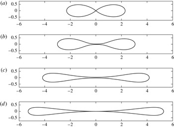
Figure 11. A plot of the closest shapes to pinch-off for various sheet and vorticity strengths. (a) The vortex patch shape, with
 $\unicode[STIX]{x1D6EC}=1$
, using 512 points (see figure 3
c). (b) The last converged Sadovskii shape with
$\unicode[STIX]{x1D6EC}=1$
, using 512 points (see figure 3
c). (b) The last converged Sadovskii shape with
 $\unicode[STIX]{x1D6EC}=0.62533$
, using 128 points. (c) The last converged Sadovskii shape with
$\unicode[STIX]{x1D6EC}=0.62533$
, using 128 points. (c) The last converged Sadovskii shape with
 $\unicode[STIX]{x1D6EC}=0.29238$
, using 256 points. (d) The theoretical limit for the vortex sheet, from Llewellyn Smith & Crowdy (Reference Llewellyn Smith and Crowdy2012) (see figure 7).
$\unicode[STIX]{x1D6EC}=0.29238$
, using 256 points. (d) The theoretical limit for the vortex sheet, from Llewellyn Smith & Crowdy (Reference Llewellyn Smith and Crowdy2012) (see figure 7).

Figure 12. The shapes of Sadovskii vortices at the
 $m=3$
bifurcation point at three different locations on the solution manifold. (a) The vortex at the bifurcation point for
$m=3$
bifurcation point at three different locations on the solution manifold. (a) The vortex at the bifurcation point for
 $\unicode[STIX]{x1D6EC}=0.98807$
and
$\unicode[STIX]{x1D6EC}=0.98807$
and
 $S_{r}=0.02110$
. (b) The vortex at
$S_{r}=0.02110$
. (b) The vortex at
 $\unicode[STIX]{x1D6EC}=0.74368$
and
$\unicode[STIX]{x1D6EC}=0.74368$
and
 $S_{r}=0.01555$
. (c) The vortex at
$S_{r}=0.01555$
. (c) The vortex at
 $\unicode[STIX]{x1D6EC}=0.53038$
and
$\unicode[STIX]{x1D6EC}=0.53038$
and
 $S_{r}=0.01192$
.
$S_{r}=0.01192$
.
5.3.1 Bifurcation for
$m=3$

While the bifurcation point for
 $m=4$
caused a split in the solution families for
$m=4$
caused a split in the solution families for
 $\unicode[STIX]{x1D6EC}<1$
, the asymmetric bifurcating family for
$\unicode[STIX]{x1D6EC}<1$
, the asymmetric bifurcating family for
 $m=3$
remained attached to the connecting family. This pattern of splitting of families at even-numbered values of
$m=3$
remained attached to the connecting family. This pattern of splitting of families at even-numbered values of
 $m$
, while the bifurcating families at odd values of
$m$
, while the bifurcating families at odd values of
 $m$
remain attached to the family, seems to continue for higher values of
$m$
remain attached to the family, seems to continue for higher values of
 $m$
on other branches.
$m$
on other branches.
Figure 12 shows the vortex shapes at the
 $m=3$
bifurcation point for three different points on the solution manifold. As the bifurcation points move to smaller values of the shape parameter and strain ratio, they take on more of the characteristics of the shapes that were originally on the bifurcating branch for
$m=3$
bifurcation point for three different points on the solution manifold. As the bifurcation points move to smaller values of the shape parameter and strain ratio, they take on more of the characteristics of the shapes that were originally on the bifurcating branch for
 $m=4$
(see figure 3
a), showing the flattening out and then beginnings of the pinch-off in the centre.
$m=4$
(see figure 3
a), showing the flattening out and then beginnings of the pinch-off in the centre.
To calculate the shapes of the asymmetric vortices on the bifurcating families for
 $m=3$
, we calculated a perturbed solution near the bifurcation point, then used this perturbed solution as a starting point for continuation in
$m=3$
, we calculated a perturbed solution near the bifurcation point, then used this perturbed solution as a starting point for continuation in
 $\unicode[STIX]{x1D707}$
. Using increased weights on the centroid and area constraints (
$\unicode[STIX]{x1D707}$
. Using increased weights on the centroid and area constraints (
 $a=b=c=10^{5}$
instead of 100) gave better convergence to solutions.
$a=b=c=10^{5}$
instead of 100) gave better convergence to solutions.
In the vortex patch case, the limiting shape for this solution branch had a cusp, shown in figure 13(a). As the vortex sheet strength increases, the vortex can no longer support a cusp. Instead, the effect of the sheet is to round the cusp out, and it begins to extend in a thin finger. As the straining field and vortex sheet become stronger (but remain in the large
 $\unicode[STIX]{x1D6EC}$
regime), this thin finger also begins to curve. This shape is shown in figure 13(b).
$\unicode[STIX]{x1D6EC}$
regime), this thin finger also begins to curve. This shape is shown in figure 13(b).

Figure 13. Comparison of patch and Sadovskii asymmetric shapes. (a) The limiting shape for the patch vortex (
 $\unicode[STIX]{x1D6EC}=1$
) showing the cusp. This comes from the bifurcating family for
$\unicode[STIX]{x1D6EC}=1$
) showing the cusp. This comes from the bifurcating family for
 $m=3$
. (b) The last converging shape for the related bifurcating family at (
$m=3$
. (b) The last converging shape for the related bifurcating family at (
 $\unicode[STIX]{x1D6EC}=0.93196$
,
$\unicode[STIX]{x1D6EC}=0.93196$
,
 $S_{r}=0.02051$
). The vortex sheet forces a round shape, and in this case begins to extend the side where the cusp was. There is also a slight curve to the narrow finger that occurs where the cusp was. This curve becomes more pronounced with increasing
$S_{r}=0.02051$
). The vortex sheet forces a round shape, and in this case begins to extend the side where the cusp was. There is also a slight curve to the narrow finger that occurs where the cusp was. This curve becomes more pronounced with increasing
 $S_{r}$
.
$S_{r}$
.
As
 $\unicode[STIX]{x1D6EC}$
decreases (and the sheet strength increases), the vortex shape becomes more rounded, with a wider minimum width. Figure 14(a) shows the symmetric solution at the bifurcation point when nearly half the circulation is due to the vortex sheet. Figure 14(b) shows the last converged asymmetric solution on the bifurcating branch, showing the wider radius of curvature where the cusp or finger existed in vortices with weaker vortex sheets (figure 13). We calculated the asymmetric solutions for many solution families that had the bifurcation point, but did not attempt to discover where these asymmetric families ceased to exist as
$\unicode[STIX]{x1D6EC}$
decreases (and the sheet strength increases), the vortex shape becomes more rounded, with a wider minimum width. Figure 14(a) shows the symmetric solution at the bifurcation point when nearly half the circulation is due to the vortex sheet. Figure 14(b) shows the last converged asymmetric solution on the bifurcating branch, showing the wider radius of curvature where the cusp or finger existed in vortices with weaker vortex sheets (figure 13). We calculated the asymmetric solutions for many solution families that had the bifurcation point, but did not attempt to discover where these asymmetric families ceased to exist as
 $\unicode[STIX]{x1D6EC}$
tends to zero.
$\unicode[STIX]{x1D6EC}$
tends to zero.

Figure 14. Asymmetric branch for a Sadovskii vortex. (a) The symmetric shape at the bifurcation point (
 $\unicode[STIX]{x1D6EC}=0.53038$
,
$\unicode[STIX]{x1D6EC}=0.53038$
,
 $S_{R}=0.01192$
). (b) The last converged shape for the Sadovskii vortex (
$S_{R}=0.01192$
). (b) The last converged shape for the Sadovskii vortex (
 $\unicode[STIX]{x1D6EC}=0.52351$
,
$\unicode[STIX]{x1D6EC}=0.52351$
,
 $S_{r}=0.01191$
) showing the asymmetry. This comes from the bifurcating family for
$S_{r}=0.01191$
) showing the asymmetry. This comes from the bifurcating family for
 $m=3$
.
$m=3$
.
5.4 Branches for
$m=4$
and
$m=6$


The natures of the
 $m=4$
and
$m=4$
and
 $m=6$
bifurcation points are the same: the top family of more circular vortices remains attached to the family with pinch-offs, while the family of patch vortices with sharp cusps becomes attached to the lower family of more elongated shapes. Now the lower family (dashed line) in figure 9 is attached to the family with two pinch-off points (see figure 15). However, neither of these families exists all the way to
$m=6$
bifurcation points are the same: the top family of more circular vortices remains attached to the family with pinch-offs, while the family of patch vortices with sharp cusps becomes attached to the lower family of more elongated shapes. Now the lower family (dashed line) in figure 9 is attached to the family with two pinch-off points (see figure 15). However, neither of these families exists all the way to
 $\unicode[STIX]{x1D6EC}=0$
. The separation is shown in figure 15, while the family between
$\unicode[STIX]{x1D6EC}=0$
. The separation is shown in figure 15, while the family between
 $m=4$
and
$m=4$
and
 $m=6$
are shown in figure 16.
$m=6$
are shown in figure 16.

Figure 15. Split in Sadovskii vortex families near the
 $m=6$
bifurcation point. (a) Patch solutions with
$m=6$
bifurcation point. (a) Patch solutions with
 $\unicode[STIX]{x1D706}=0$
. (b–d) Sadovskii solutions at constant values of
$\unicode[STIX]{x1D706}=0$
. (b–d) Sadovskii solutions at constant values of
 $\unicode[STIX]{x1D706}=0.05051$
, 0.07191 and 0.08880, respectively. The family between
$\unicode[STIX]{x1D706}=0.05051$
, 0.07191 and 0.08880, respectively. The family between
 $m=4$
and
$m=4$
and
 $m=6$
is shown by the solid line and the more elongated family is shown by the dashed line. As
$m=6$
is shown by the solid line and the more elongated family is shown by the dashed line. As
 $\unicode[STIX]{x1D706}$
increases, these families get farther from each other.
$\unicode[STIX]{x1D706}$
increases, these families get farther from each other.

Figure 16. The family of Sadovskii solutions connecting the doubly cusped solutions at the
 $m=4$
patch bifurcation with the solutions with two pinch-off points at the
$m=4$
patch bifurcation with the solutions with two pinch-off points at the
 $m=6$
patch bifurcation is shown in the darker color. All other Sadovskii solutions are shown in lighter grey.
$m=6$
patch bifurcation is shown in the darker color. All other Sadovskii solutions are shown in lighter grey.
The behaviour of the cusps is similar to the single cusp in the
 $m=3$
branch. In this case, it occurs on both sides, and it does not appear to exhibit the slight curve shown in figure 13(b). As the sheet strength is increased, thin fingers again extend outwards from where the cusps were. As the sheet continues to increase in strength, these fingers get wider at the edges, and the shape appears closely related to one with two pinch-off points (see figure 18). As the sheet strength increases, there is less variance in vortex shape between the edges of the family. In figure 17, we show the cusped patch shape and compare it to a Sadovskii shape showing the bulging fingers on both ends.
$m=3$
branch. In this case, it occurs on both sides, and it does not appear to exhibit the slight curve shown in figure 13(b). As the sheet strength is increased, thin fingers again extend outwards from where the cusps were. As the sheet continues to increase in strength, these fingers get wider at the edges, and the shape appears closely related to one with two pinch-off points (see figure 18). As the sheet strength increases, there is less variance in vortex shape between the edges of the family. In figure 17, we show the cusped patch shape and compare it to a Sadovskii shape showing the bulging fingers on both ends.

Figure 17. Comparison of patch and Sadovskii shapes for
 $m=4$
branch. (a) The limiting shape for the patch vortex (
$m=4$
branch. (a) The limiting shape for the patch vortex (
 $\unicode[STIX]{x1D6EC}=1$
,
$\unicode[STIX]{x1D6EC}=1$
,
 $\unicode[STIX]{x1D707}=0.06072$
) showing the cusps (see figure 3
d). (b) The last converging shape for the related bifurcating family at (
$\unicode[STIX]{x1D707}=0.06072$
) showing the cusps (see figure 3
d). (b) The last converging shape for the related bifurcating family at (
 $\unicode[STIX]{x1D6EC}=0.75920$
,
$\unicode[STIX]{x1D6EC}=0.75920$
,
 $S_{r}=0.01326$
). The vortex sheet forces a round shape, which leads to the skinny fingers on each side where the cusps had been. This shape is the end of the family of solutions represented by the dashed lines in figure 9.
$S_{r}=0.01326$
). The vortex sheet forces a round shape, which leads to the skinny fingers on each side where the cusps had been. This shape is the end of the family of solutions represented by the dashed lines in figure 9.
As figure 18 shows, as the vortex sheet strength increases, the pinch-off points on the
 $m=6$
branch are smoothed out much as occurs in the hollow case. No solutions for
$m=6$
branch are smoothed out much as occurs in the hollow case. No solutions for
 $\unicode[STIX]{x1D6EC}<0.6$
converged for this family between
$\unicode[STIX]{x1D6EC}<0.6$
converged for this family between
 $m=4$
and
$m=4$
and
 $m=6$
. It is likely that this family ends at a point where the only solution is at the
$m=6$
. It is likely that this family ends at a point where the only solution is at the
 $m=5$
bifurcation point.
$m=5$
bifurcation point.

Figure 18. Comparison of patch and Sadovskii shapes for
 $m=6$
branch. (a) The limiting shape for the patch vortex (
$m=6$
branch. (a) The limiting shape for the patch vortex (
 $\unicode[STIX]{x1D6EC}=1$
,
$\unicode[STIX]{x1D6EC}=1$
,
 $\unicode[STIX]{x1D707}=0.03358$
) showing the sharp pinch points (see figure 5
c). (b) The last converging shape for the related bifurcating family at (
$\unicode[STIX]{x1D707}=0.03358$
) showing the sharp pinch points (see figure 5
c). (b) The last converging shape for the related bifurcating family at (
 $\unicode[STIX]{x1D6EC}=0.71162$
,
$\unicode[STIX]{x1D6EC}=0.71162$
,
 $S_{r}=0.00775$
). The vortex sheet leads to pinch-off points that are closer to those of the hollow vortex, or the vortex sheet alone.
$S_{r}=0.00775$
). The vortex sheet leads to pinch-off points that are closer to those of the hollow vortex, or the vortex sheet alone.
As
 $\unicode[STIX]{x1D6EC}$
is decreased, the shape of the vortices at the bifurcation point begins to show the signature of two pinch-off locations, as shown in figure 19. The two shapes, one with the two sharp ends, and one with the two pinch-off points, become more similar as the vortex sheet becomes stronger, as can be seen from the shape of figure 19(b).
$\unicode[STIX]{x1D6EC}$
is decreased, the shape of the vortices at the bifurcation point begins to show the signature of two pinch-off locations, as shown in figure 19. The two shapes, one with the two sharp ends, and one with the two pinch-off points, become more similar as the vortex sheet becomes stronger, as can be seen from the shape of figure 19(b).

Figure 19. Sadovskii vortex shapes for
 $m=5$
bifurcation points. (a) The shape at
$m=5$
bifurcation points. (a) The shape at
 $\unicode[STIX]{x1D6EC}=0.98070$
and
$\unicode[STIX]{x1D6EC}=0.98070$
and
 $S_{r}=0.015224$
. (b) The shape at
$S_{r}=0.015224$
. (b) The shape at
 $\unicode[STIX]{x1D6EC}=0.76783$
and
$\unicode[STIX]{x1D6EC}=0.76783$
and
 $S_{r}=0.01134$
.
$S_{r}=0.01134$
.
Figure 20 shows the asymmetric shape of a vortex on the bifurcating family, at
 $\unicode[STIX]{x1D6EC}=0.76452$
,
$\unicode[STIX]{x1D6EC}=0.76452$
,
 $S_{r}=0.01190$
. One side looks like the symmetric shape in figure 19(b), while the other side looks more like the shape in figure 17(b).
$S_{r}=0.01190$
. One side looks like the symmetric shape in figure 19(b), while the other side looks more like the shape in figure 17(b).

Figure 20. Sadovskii vortex asymmetric shape at the
 $m=5$
bifurcation point, with
$m=5$
bifurcation point, with
 $\unicode[STIX]{x1D6EC}=0.76452$
and
$\unicode[STIX]{x1D6EC}=0.76452$
and
 $S_{r}=0.01190$
. One side of this asymmetric vortex looks like the shape on the symmetric family, while the other side is narrower. Compare this to the patch shape in figure 4(b).
$S_{r}=0.01190$
. One side of this asymmetric vortex looks like the shape on the symmetric family, while the other side is narrower. Compare this to the patch shape in figure 4(b).
6 Conclusions
We have obtained the shapes of steady Sadovskii vortices in strain. Using numerical continuation, we were able to trace out the solution manifold described by two parameters, taken here to be
 $\unicode[STIX]{x1D6EC}=\unicode[STIX]{x1D6E4}_{in}/\unicode[STIX]{x1D6E4}_{out}$
and
$\unicode[STIX]{x1D6EC}=\unicode[STIX]{x1D6E4}_{in}/\unicode[STIX]{x1D6E4}_{out}$
and
 $S_{r}=\unicode[STIX]{x1D6FE}L^{2}/\unicode[STIX]{x1D6E4}_{out}$
. The limiting cases of the vortex patch and vortex sheet are recovered and match previously obtained solutions.
$S_{r}=\unicode[STIX]{x1D6FE}L^{2}/\unicode[STIX]{x1D6E4}_{out}$
. The limiting cases of the vortex patch and vortex sheet are recovered and match previously obtained solutions.
For vortex patches, we obtained families that bifurcate from the elliptical solutions, as in Kamm (Reference Kamm1987). We took the calculations further than before, and found that families at higher values of
 $m$
had more pinch-offs. Even bifurcation points led to asymmetric vortex shapes that extended only into larger values of
$m$
had more pinch-offs. Even bifurcation points led to asymmetric vortex shapes that extended only into larger values of
 $S_{r}$
. Odd bifurcation points lead to families that extend in both directions along
$S_{r}$
. Odd bifurcation points lead to families that extend in both directions along
 $S_{r}$
, with either a pinch-off point or a sharp cusp at either end.
$S_{r}$
, with either a pinch-off point or a sharp cusp at either end.
For Sadovskii vortices, we calculated points on the solution manifold in the parameter space. The addition of the vortex sheet to the vortex patch solutions immediately leads to a split in the solution manifold at bifurcation points for even values of
 $m$
. It is this splitting of the families that leads to the much simpler solution branch for the vortex sheet. The more circular vortex patch solutions remain connected to the family with a single pinch-off at
$m$
. It is this splitting of the families that leads to the much simpler solution branch for the vortex sheet. The more circular vortex patch solutions remain connected to the family with a single pinch-off at
 $m=4$
, while becoming disconnected from the more elongated elliptical solutions and the family with cusps at both ends.
$m=4$
, while becoming disconnected from the more elongated elliptical solutions and the family with cusps at both ends.
The addition of the vortex sheet to the vortex patch smooths out sharp features. As the vortex sheet strength is increased, the radius of curvature also increases, so features such as fingers become wider and less pronounced. This leads to a shrinking of the solution manifold, as the more deformed shapes do not seem to exist for strong enough vortex sheet strengths and the existing shapes become more similar. It also appears that the more elongated families that exist below the
 $m=4$
family only exist for small values of the vortex sheet strength, which explains why they do not appear as vortex sheet solutions.
$m=4$
family only exist for small values of the vortex sheet strength, which explains why they do not appear as vortex sheet solutions.
We have shown that our approach successfully calculates the known vortex patch and sheet shapes and used it to find new shapes. It can also be applied to cases with rotational background flows by decomposing the flow appropriately. For example, it can be used to obtain the hollow vortex in shear solutions of Zannetti, Ferlauto & Llewellyn Smith (Reference Zannetti, Ferlauto and Llewellyn Smith2016). Other possible situations include multiple vortex equilibria to desingularize the classical rotating same-sign point vortices.
Future work may investigate the stability of the steady solutions we have calculated. This will be particularly interesting in the presence of surface tension, which may serve to mitigate the possibility of Kelvin–Helmholtz instability in the stagnant case when the inner fluid has non-zero density.
Acknowledgements
This work was partially supported by NSF award CMMI-0970113. A UCSD Collaboratory award also provided support. Helpful discussions with D. Crowdy, S. Tanveer and P. Luzzatto-Fegiz are acknowledged.
Appendix A. Numerical method
Numerical continuation is performed using a predictor–corrector scheme for pseudo-arclength continuation. For details on such schemes, see Govaerts (Reference Govaerts2000). Since we use an inverse velocity formulation, points are clustered in areas where the speed on the vortex sheet is lower. The inverse velocity discretization (see Luzzatto-Fegiz & Williamson Reference Luzzatto-Fegiz and Williamson2011) is
 $$\begin{eqnarray}\tilde{s}(s)=A\int _{0}^{s}\frac{\text{d}s^{\prime }}{|\boldsymbol{u}(s^{\prime })|},\end{eqnarray}$$
where
 $A$
is chosen so
$A$
is chosen so
 $0\leqslant \tilde{s}\leqslant 2\unicode[STIX]{x03C0}$
,
$0\leqslant \tilde{s}\leqslant 2\unicode[STIX]{x03C0}$
,
 $s$
is the arclength and
$s$
is the arclength and
 $\boldsymbol{u}$
is the velocity in the reference frame of interest. This method assumes that the solution is a superposition of three velocity fields: the background straining flow, the vortex patch and the vortex sheet. Given a vortex solution, the basic method for the continuation is:
$\boldsymbol{u}$
is the velocity in the reference frame of interest. This method assumes that the solution is a superposition of three velocity fields: the background straining flow, the vortex patch and the vortex sheet. Given a vortex solution, the basic method for the continuation is:
-
(i) rediscretize points by inverse velocity using cubic splines;
-
(ii) predict new vortex solution using the null space of Jacobian;
-
(iii) correct the guess using the Gauss–Newton solver to converge to the actual solution;
-
(iv) repeat until convergence is achieved.
To reduce the number of variables in the problem, the boundary points of the vortex are only allowed to move along the normal vectors. We are calculating the scalar functions
 $\unicode[STIX]{x1D6FC}$
and
$\unicode[STIX]{x1D6FC}$
and
 $\unicode[STIX]{x1D6FC}_{k}$
, where
$\unicode[STIX]{x1D6FC}_{k}$
, where
 $$\begin{eqnarray}\displaystyle x_{i}^{n} & = & \displaystyle x_{i}+\unicode[STIX]{x1D6FC}(\tilde{s}_{i})n_{x},\end{eqnarray}$$
 $$\begin{eqnarray}\displaystyle y_{i}^{n} & = & \displaystyle y_{i}+\unicode[STIX]{x1D6FC}(\tilde{s}_{i})n_{y},\end{eqnarray}$$
 $$\begin{eqnarray}\displaystyle \unicode[STIX]{x1D705}_{i}^{n} & = & \displaystyle \unicode[STIX]{x1D705}_{i}+\unicode[STIX]{x1D6FC}_{\unicode[STIX]{x1D705}}(\tilde{s}_{i}).\end{eqnarray}$$
The
 $(x_{i},y_{i})$
are the boundary points and
$(x_{i},y_{i})$
are the boundary points and
 $\unicode[STIX]{x1D705}_{i}$
represent the vortex sheet strengths at the point. The functions
$\unicode[STIX]{x1D705}_{i}$
represent the vortex sheet strengths at the point. The functions
 $\unicode[STIX]{x1D6FC}$
and
$\unicode[STIX]{x1D6FC}$
and
 $\unicode[STIX]{x1D6FC}_{\unicode[STIX]{x1D705}}$
are calculated based on their Fourier coefficients, where
$\unicode[STIX]{x1D6FC}_{\unicode[STIX]{x1D705}}$
are calculated based on their Fourier coefficients, where
 $$\begin{eqnarray}\unicode[STIX]{x1D6FC}(\tilde{s}_{i})=\frac{1}{N}\mathop{\sum }_{j=-N/2}^{N/2-1}\hat{\unicode[STIX]{x1D6FC}}_{j}\text{e}^{2\unicode[STIX]{x03C0}\tilde{s}_{i}j\text{i}/N},\end{eqnarray}$$
with
 $\hat{\unicode[STIX]{x1D6FC}}_{j}$
the complex Fourier coefficients. While we define the shapes using
$\hat{\unicode[STIX]{x1D6FC}}_{j}$
the complex Fourier coefficients. While we define the shapes using
 $N$
points, we only allow
$N$
points, we only allow
 $M$
modes in the adjustment functions
$M$
modes in the adjustment functions
 $\unicode[STIX]{x1D6FC}$
and
$\unicode[STIX]{x1D6FC}$
and
 $\unicode[STIX]{x1D6FC}_{\unicode[STIX]{x1D705}}$
, where
$\unicode[STIX]{x1D6FC}_{\unicode[STIX]{x1D705}}$
, where
 $M\leqslant N$
, so we require that
$M\leqslant N$
, so we require that
 $\hat{\unicode[STIX]{x1D6FC}}_{j}=0$
for
$\hat{\unicode[STIX]{x1D6FC}}_{j}=0$
for
 $|\,j|>M$
. We are using
$|\,j|>M$
. We are using
 $M$
as a way to set the maximum wavenumber we keep when we apply an ideal low-pass filter to the adjustment of the shape. A similar approach is used for
$M$
as a way to set the maximum wavenumber we keep when we apply an ideal low-pass filter to the adjustment of the shape. A similar approach is used for
 $\unicode[STIX]{x1D6FC}_{\unicode[STIX]{x1D705}}$
. The unknowns that are actually found by the predictor–corrector method are the Fourier coefficients
$\unicode[STIX]{x1D6FC}_{\unicode[STIX]{x1D705}}$
. The unknowns that are actually found by the predictor–corrector method are the Fourier coefficients
 $\hat{\unicode[STIX]{x1D6FC}}$
and
$\hat{\unicode[STIX]{x1D6FC}}$
and
 $\hat{\unicode[STIX]{x1D6FC}}_{\unicode[STIX]{x1D705}}$
.
$\hat{\unicode[STIX]{x1D6FC}}_{\unicode[STIX]{x1D705}}$
.
The two boundary conditions used to calculate these Fourier coefficients are the Fourier transforms of the kinematic condition (2.6) and the dynamic (Bernoulli) condition (2.9). The total velocity is
 $\boldsymbol{u}=\boldsymbol{u}_{patch}+\boldsymbol{u}_{sheet}+\boldsymbol{u}_{strain}$
, where
$\boldsymbol{u}=\boldsymbol{u}_{patch}+\boldsymbol{u}_{sheet}+\boldsymbol{u}_{strain}$
, where
 $\boldsymbol{u}_{patch}$
is calculated from (3.3) and
$\boldsymbol{u}_{patch}$
is calculated from (3.3) and
 $\boldsymbol{u}_{sheet}$
is calculated from (4.2). The integrals in these calculations are calculated using the trapezoidal rule, applied at the midpoints to avoid poles at the points of interest. The values at midpoints are calculated using Fourier transforms, as in Baker & Nachbin (Reference Baker and Nachbin1998). Just as the average velocity on the vortex boundary is used for the discretization of the points, the same average velocity, which is the principal value integral in (4.2), is used in the kinematic condition. This works because the additional term that comes from the vortex sheet cannot affect the normal velocity.
$\boldsymbol{u}_{sheet}$
is calculated from (4.2). The integrals in these calculations are calculated using the trapezoidal rule, applied at the midpoints to avoid poles at the points of interest. The values at midpoints are calculated using Fourier transforms, as in Baker & Nachbin (Reference Baker and Nachbin1998). Just as the average velocity on the vortex boundary is used for the discretization of the points, the same average velocity, which is the principal value integral in (4.2), is used in the kinematic condition. This works because the additional term that comes from the vortex sheet cannot affect the normal velocity.
Depending on the solution regime, different non-dimensionalizations of these boundary conditions were used. For solutions near the vortex patch, the equations were non-dimensionalized using
 $$\begin{eqnarray}x=Lx^{\ast },\quad u=L\unicode[STIX]{x1D714}u^{\ast },\quad \unicode[STIX]{x1D707}=\frac{\unicode[STIX]{x1D6FE}}{\unicode[STIX]{x1D714}},\quad \unicode[STIX]{x1D706}=\frac{q}{\unicode[STIX]{x1D714}L},\quad \unicode[STIX]{x1D70C}=\frac{\unicode[STIX]{x1D70C}_{i}}{\unicode[STIX]{x1D70C}_{o}},\end{eqnarray}$$
while solutions near the vortex sheet were non-dimensionalized using
 $$\begin{eqnarray}x=Lx^{\ast },\quad u=L\unicode[STIX]{x1D6FE}u^{\ast },\quad \unicode[STIX]{x1D707}_{s}=\frac{\unicode[STIX]{x1D714}}{\unicode[STIX]{x1D6FE}},\quad \unicode[STIX]{x1D706}_{s}=\frac{\unicode[STIX]{x1D6FE}L}{q},\quad \unicode[STIX]{x1D70C}=\frac{\unicode[STIX]{x1D70C}_{i}}{\unicode[STIX]{x1D70C}_{o}}.\end{eqnarray}$$
These non-dimensionalizations are used for numerical purposes and are not needed in the discussion of § 5.
We actually solve a constrained problem, in which each of the boundary conditions has added terms to ensure the vortex is centred at the origin and has a fixed area. The area and centroids are calculated using the trapezoidal rule from
 $$\begin{eqnarray}A=\oint x\,\frac{\text{d}y}{\text{d}\tilde{s}}\,\text{d}\tilde{s},\quad x_{C}=-\frac{1}{2A}\oint x^{2}\,\frac{\text{d}y}{\text{d}\tilde{s}}\,\text{d}\tilde{s},\quad y_{C}=\frac{1}{2A}\oint y^{2}\,\frac{\text{d}x}{\text{d}\tilde{s}}\,\text{d}\tilde{s}.\end{eqnarray}$$
The constraints added to (2.6) and (2.9) are
 $$\begin{eqnarray}ax_{c}t_{1}(s_{r})+by_{c}t_{2}(s_{r})+c(A-\unicode[STIX]{x03C0})t_{3}(s_{r})=0,\end{eqnarray}$$
where
 $a,~b$
and
$a,~b$
and
 $c$
are weights and
$c$
are weights and
 $t_{1}$
,
$t_{1}$
,
 $t_{2}$
and
$t_{2}$
and
 $t_{3}$
are the first three Legendre polynomials evaluated at
$t_{3}$
are the first three Legendre polynomials evaluated at
 $s_{r}=(\tilde{s}/\unicode[STIX]{x03C0})-1$
. We used weights of
$s_{r}=(\tilde{s}/\unicode[STIX]{x03C0})-1$
. We used weights of
 $a=b=c=100$
, unless otherwise noted, to ensure that the area and centroid conditions were satisfied. These constraints are added before the Fourier transform is taken.
$a=b=c=100$
, unless otherwise noted, to ensure that the area and centroid conditions were satisfied. These constraints are added before the Fourier transform is taken.
Results were checked to make sure the area and centroid constraints were satisfied. After reviewing the results, we found that high-frequency Nyquist mode oscillations or non-physical (self-intersecting) shapes occurred when
 $|x_{c}|>5\times 10^{-7}$
,
$|x_{c}|>5\times 10^{-7}$
,
 $|y_{c}|>5\times 10^{-7}$
or
$|y_{c}|>5\times 10^{-7}$
or
 $|A-\unicode[STIX]{x03C0}|>5\times 10^{-6}$
. Only solutions with centroid and area errors smaller than these values were retained.
$|A-\unicode[STIX]{x03C0}|>5\times 10^{-6}$
. Only solutions with centroid and area errors smaller than these values were retained.
Branch switching was performed by solving a perturbed problem, where a constant term was added to the boundary conditions. This perturbation causes a splitting of the families at the bifurcation point, allowing continuation to go smoothly from one branch to the other. Once on the other branch, the perturbation was removed and the actual problem was solved, using as a starting guess the perturbed solution on the new branch.


