


1. Introduction
Figure 1 depicts an annular heater travelling at speed  $\mathcal {V}$ along a long annular silica-glass capillary with initial external radius
  $\mathcal {R}_{{I}}$, and aspect ratio
  $\phi _I$ defined as the ratio of the internal and external radii such that the internal radius is
  $\phi _I\mathcal {R}_{{I}}$. The initial cross-sectional area of the capillary is
  $\mathcal {S}_{{I}}={\rm \pi} \mathcal {R}_{{I}}^{2}(1-\phi _I^{2})$. At any time
  $t$, a length
  $\mathcal {L}$ of the capillary (commensurate with but not necessarily equal to the physical heater length) is heated and softened such that the glass is a viscous liquid and surface tension acts to collapse the capillary. After the heater has passed and the capillary has cooled to a solid it has final external radius
  $\mathcal {R}_{{F}}<\mathcal {R}_{{I}}$ and aspect ratio
  $\phi _F<\phi _I$. The extent of collapse of the capillary is used, with a suitable mathematical model, to determine the (possibly temperature-dependent) surface tension or viscosity of silica glasses (Kirchhof Reference Kirchhof1985a,Reference Kirchhofb; Kirchhof & Unger Reference Kirchhof and Unger2017; Klupsch & Pan Reference Klupsch and Pan2017).

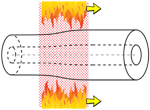
Figure 1. Schematic diagram of the collapse of a capillary (a) in the laboratory reference frame where a heater travels to the right at speed  $\mathcal {V}$ along the capillary resulting in a moving heated region of length
  $\mathcal {L}$, and (b) in the reference frame moving with the heater in which the capillary moves to the left at speed
  $\mathcal {V}$ through the stationary heated region of length
  $\mathcal {L}$. A cross-section of the capillary enters the heated region with initial external radius
  $\mathcal {R}_{{I}}$ and aspect ratio
  $\phi _I$, and exits the heated region with external radius
  $\mathcal {R}_{{F}}$ and aspect ratio
  $\phi _F$. Beyond the heated region the capillary is solid. In the moving reference frame the
  $x$-axis is directed along the axis of the capillary in the direction of increasing collapse with the centre of the heated region at
  $x=0$.
Capillary collapse is also used in the manufacture of optical fibre preforms by modified chemical vapour deposition; following the deposition of glassy films from a flow of gaseous reactants through the capillary while heating using a travelling heater, the capillary is then further heated so that it collapses to a solid multi-material rod which may be drawn to a fibre (Lewis Reference Lewis1977; Kirchhof Reference Kirchhof1980; Geyling, Walker & Csencsits Reference Geyling, Walker and Csencsits1983; Kirchhof Reference Kirchhof1985a; Das & Gandhi Reference Das and Gandhi1986; Kirchhof & Unger Reference Kirchhof and Unger2017). Since capillary collapse during the vapour deposition phase affects the gas flow and chemical kinetics, a mathematical model is important for understanding of this phase, as well as to predict the heating needed to achieve a solid rod in the second phase.
The deformation over time under surface tension of an annular cross-section of a capillary, ignoring any flow in the axial direction (normal to the cross-section), is the simplest, most common and oldest model used for capillary collapse as described above (Lewis Reference Lewis1977; Kirchhof Reference Kirchhof1985a,Reference Kirchhofb; Klupsch & Pan Reference Klupsch and Pan2017; Kirchhof & Unger Reference Kirchhof and Unger2017). Axisymmetry of the capillary means that the model may be written in terms of one spatial variable, the radius  $r$, so that it is called ‘the one-dimensional (1-D) model’. The cross-sectional area remains constant, the surface tension
  $\gamma$, which is only weakly temperature-dependent, is assumed to be constant and the fluid viscosity
  $\mu$, which is strongly dependent on temperature, is assumed to be spatially uniform and to depend only on time
  $t$. This problem has an analytic solution. Note that this 1-D model has also been used for capillary collapse due to a stationary heater (
 $\mathcal {V}=0$) (Makovetskii, Zamyatin & Ivanov Reference Makovetskii, Zamyatin and Ivanov2013). A radially dependent viscosity was considered by Geyling et al. (Reference Geyling, Walker and Csencsits1983) who also relaxed the assumption of radial symmetry and, hence, used a two-dimensional (2-D) model of the annular cross-section in polar coordinates
  $(r,\theta )$.
The first 2-D axisymmetric model developed explicitly for capillary collapse, accounting for motion in both radial and axial directions, seems to be that of Klupsch & Pan (Reference Klupsch and Pan2017). For a capillary held fixed at both ends, and assuming that the length scale in the radial direction is small relative to the length scale in the axial direction, they performed an ‘asymptotic multiscale analysis’ to obtain a 2-D description of capillary collapse. Comparison of this with the 1-D model and finite element simulations found that the difference between the 1-D and 2-D models was ‘marginal’.
However, in the reference frame moving with the heater a capillary held fixed at both ends travels through the now stationary heater (see figure 1). This problem is essentially identical to the Vello process for manufacturing capillary tubing modelled by Griffiths & Howell (Reference Griffiths and Howell2008), and differs from the drawing of tubular fibres only because the capillary enters and exits the heated region at the same speed  $\mathcal {V}$, i.e. it is fibre drawing with unit draw ratio. Extensive attention has been given over three decades to mathematical modelling of the drawing of slender microstructured optical fibres, incorporating both axial and cross-sectional flow (Yarin et al. Reference Yarin, Rusinov, Gospodinov and Radev1989; Yarin, Gospodinov & Rusinov Reference Yarin, Gospodinov and Rusinov1994; Fitt et al. Reference Fitt, Furusawa, Monro, Please and Richardson2002; Griffiths & Howell Reference Griffiths and Howell2008; Stokes et al. Reference Stokes, Buchak, Crowdy and Ebendorff-Heidepriem2014; Chen et al. Reference Chen, Stokes, Buchak, Crowdy and Ebendorff-Heidepriem2015; Xue et al. Reference Xue, Tanner, Barton, Lwin, Large and Poladian2015a,Reference Xue, Tanner, Barton, Lwin, Large and Poladianb; Chen et al. Reference Chen, Stokes, Buchak, Crowdy and Ebendorff-Heidepriem2016b; Stokes, Wylie & Chen Reference Stokes, Wylie and Chen2019), and the drawing of slender axisymmetric tubes is a particular case. Thus, 2-D models exist which are applicable to capillary collapse and which predate that of Klupsch & Pan (Reference Klupsch and Pan2017). For a radial length scale that is much smaller than the axial length scale, as assumed by Klupsch & Pan, the asymptotic fibre-drawing model of Stokes et al. (Reference Stokes, Buchak, Crowdy and Ebendorff-Heidepriem2014, Reference Stokes, Wylie and Chen2019) may be used for capillary collapse and yields analytic formulae relating the extent of collapse to the harmonic mean of the viscosity and the surface tension of the glass. The accuracy of this model is excellent for drawing of fibre from very slender preforms (Chen et al. Reference Chen, Stokes, Buchak, Crowdy and Ebendorff-Heidepriem2016b) and is expected to be excellent for capillary collapse which does not see the high draw ratios and sharp tapers seen in fibre drawing and which are known to cause discrepancies between models and experiments, especially when the radius of the preform is not sufficiently small relative to the neck-down length (Chen et al. Reference Chen, Stokes, Buchak, Crowdy, Foo, Dowler and Ebendorff-Heidepriem2016a).
This 2-D asymptotic fibre-drawing model with unit draw ratio is here examined for capillary collapse. Although Klupsch and Pan's work, in showing only marginal difference between 1-D and 2-D models, suggests there is no practical value in a 2-D model, an important feature of the fibre-drawing model is that it involves a pulling-tension parameter that enables both viscosity and surface tension to be determined simultaneously from a single experiment, which is not possible using the 1-D model. Moreover, the formulae yielded by the 2-D model are not significantly more complex than those of the 1-D model and are readily used. Hence, with the 2-D model, capillary collapse may be a useful and simpler alternative to the technique proposed by Boyd et al. (Reference Boyd, Ebendorff-Heidepriem, Monro and Munch2012) for determination of both surface tension and viscosity, namely using a  $\textrm {CO}_2$ laser to heat small segments of a vertically suspended glass fibre. By this means the bottom of the fibre is heated so that a glass ball forms and detaches from the fibre, the mass of which is used to compute the surface tension, while viscosity is determined from the reduction in the fibre length when heated a suitable distance above the bottom of the fibre. Thus, although the same experimental set-up might be used, different procedures are needed for each fluid property while, as we will see, both fluid properties may be determined from a single capillary-collapse experimental procedure.
We note that the way in which the ends of the capillary are supported or held does not feature in 1-D modelling of capillary collapse, so that this is not always mentioned. In the experimental set-ups of Kirchhof (Reference Kirchhof1980, Reference Kirchhof1985a), where heating is by a moving oxy-hydrogen torch and the capillary is rotated in a glass working lathe to achieve uniform heating around the perimeter of a cross-section, it is clear that the ends of the capillary are held fixed. Klupsch & Pan (Reference Klupsch and Pan2017) assume that the cold ends of the capillary are fixed in the laboratory reference frame. However, it is possible that, with use of a travelling axisymmetric heater around the tube, rotation would not be necessary and the capillary ends could be supported but allowed to slip axially. We take the opportunity in this paper, using a modification of the 2-D fibre-drawing model, to show that such a change to the way in which the capillary is held has a significant effect on capillary collapse such that the 1-D model is significantly less accurate than for the capillary with fixed ends.
The 1-D model is a component of our 2-D model and, for this reason, although derived and solved elsewhere (Stokes et al. Reference Stokes, Buchak, Crowdy and Ebendorff-Heidepriem2014; Klupsch & Pan Reference Klupsch and Pan2017; Stokes et al. Reference Stokes, Wylie and Chen2019), we start in § 2 with a brief look at the 1-D model using notation needed for our 2-D model which is then described in § 3. In § 4 we compare 1-D and 2-D models and in § 5 we show how the surface tension and viscosity of the material from which the capillary is made may be determined. We also discuss determination of the heater speed required to achieve a desired amount of collapse of the capillary. Concluding remarks are given in § 6.
2. The 1-D model
As earlier stated, the 1-D model is for the collapse under surface tension of a 2-D liquid annulus of area  $\mathcal {S}_{{I}}$, which at time
  $t=0$ has external radius
  $\mathcal {R}_{{I}}$, and aspect ratio
  $\phi _I>0$. Let
  $r$ and
  $\theta$ be the radial and azimuthal spatial coordinates and let
  $t$ denote time. The symmetry of the problem means that all quantities are independent of
  $\theta$ and there is flow in the radial direction only, with velocity denoted by
  $v(r,t)$. Let
  $p(r,t)$ be the pressure, and
  $R(t)$ and
  $\phi (t)R(t)$ be the external and internal radii of the annulus. We assume that the liquid has spatially uniform viscosity. However, the viscosity of silica glasses depends strongly on temperature, so that we have a viscosity
  $\mu (t)$ that changes with time. On the other hand the surface tension
  $\gamma$ of silica glasses is only weakly temperature dependent so that we assume this to be constant. Table 1 gives typical values of the physical parameters for capillary collapse. We denote the external and internal free-surface boundaries of the annulus by
 \begin{gather} G_e(r,t)=r-R(t)=0, \end{gather}
 \begin{gather}G_i(r,t)=\phi(t)R(t)-r=0, \end{gather}
respectively; for convenience, the total boundary is denoted  $G=G_e+G_i=0$. The curvatures
  $\kappa$ of the external and internal boundaries are
 \begin{equation} \kappa=\left\{\begin{array}{@{}ll} 1/R & \text{on}\ G_e(r,t)=0,\\ -1/(\phi R) & \text{on}\ G_i(r,t)=0. \end{array}\right. \end{equation}
Table 1. Typical physical parameter values (Das & Gandhi Reference Das and Gandhi1986; Boyd et al. Reference Boyd, Ebendorff-Heidepriem, Monro and Munch2012; Klupsch & Pan Reference Klupsch and Pan2017).

Let  $\mathcal {U}$ be the velocity scale, to be defined later,
  $\sqrt {\mathcal {S}_{{I}}}$ be the length scale, and
  $\bar {\mu }$ be a typical value of the viscosity. Assuming a slow flow with Reynolds number
 \begin{equation} {Re}=\rho\, \mathcal{U}\sqrt{\mathcal{S}_{{I}}}/\bar{\mu}\ll 1, \end{equation}
the flow is described by a classical moving-boundary Stokes-flow problem. Defining the scaled variables, denoted by primes, by
 \begin{align}
r&=\sqrt{\mathcal{S}_{{I}}}r', \quad
t=\frac{\sqrt{\mathcal{S}_{{I}}}}{\mathcal{U}}t',\quad
R=\sqrt{\mathcal{S}_{{I}}}R',\quad
\kappa=\frac{\kappa'}{\sqrt{\mathcal{S}_{{I}}}}, \quad
v=\mathcal{U}v',\notag\\
p&=\frac{\bar{\mu}\mathcal{U}}{\sqrt{\mathcal{S}_{{I}}}}p',\quad
\mu=\bar{\mu}\mu',
\end{align}
\begin{align}
r&=\sqrt{\mathcal{S}_{{I}}}r', \quad
t=\frac{\sqrt{\mathcal{S}_{{I}}}}{\mathcal{U}}t',\quad
R=\sqrt{\mathcal{S}_{{I}}}R',\quad
\kappa=\frac{\kappa'}{\sqrt{\mathcal{S}_{{I}}}}, \quad
v=\mathcal{U}v',\notag\\
p&=\frac{\bar{\mu}\mathcal{U}}{\sqrt{\mathcal{S}_{{I}}}}p',\quad
\mu=\bar{\mu}\mu',
\end{align}the dimensionless Stokes-flow model is, on dropping primes,
 \begin{gather} \frac{1}{r}\frac{\partial}{\partial r}(rv)=0, \end{gather}
 \begin{gather}-\frac{\partial p}{\partial r}+\mu\left\{\frac{1}{r}\frac{\partial}{\partial r}\left(r\frac{\partial v}{\partial r}\right)-\frac{v}{r^{2}}\right\}=0, \end{gather}
 \begin{gather}-p+2\mu\frac{\partial v}{\partial r}=-\frac{\kappa}{{Ca}}\quad \mbox{on}\ G=0, \end{gather}
 \begin{gather}\frac{\partial G}{\partial t}+v\frac{\partial G}{\partial r}=0\quad \mbox{on}\ G=0, \end{gather}
where
 \begin{equation} {Ca}={\bar{\mu}\, \mathcal{U}}/{\gamma}\end{equation}
is the capillary number. We set  $\mathcal {U}=\gamma /\bar {\mu }$ so that
  ${Ca}=1$, which is appropriate for a flow driven by surface tension. The flow domain has unit dimensionless area for all time.
This model is readily solved to give
 \begin{equation} v=-\frac{\phi R}{2\mu(1-\phi)r},\quad p=\frac{1}{R(1-\phi)}, \end{equation}
where
 \begin{equation} {\rm \pi}R^{2}(1-\phi^{2})=1\ \Rightarrow\ R=\frac{1}{\sqrt{{\rm \pi}(1-\phi^{2})}}. \end{equation}
On  $G_e=0$ and
  $G_i=0$ the kinematic condition (2.9) gives
 \begin{equation} \frac{\textrm{d}R}{\textrm{d}t}=-\frac{\phi}{2\mu(1-\phi)}, \quad \frac{\textrm{d}}{\textrm{d}t}(\phi R)=-\frac{1}{2\mu(1-\phi)}, \end{equation}
respectively, so that
 \begin{equation} \frac{\textrm{d}}{\textrm{d}t}\left\{R(1-\phi)\right\}=\frac{1}{2\mu}.\end{equation}
For convenience, we define  $\omega (t)=R(t)(1-\phi (t))$ as the wall thickness of the annulus at time
  $t$ and, on substituting for
  $R$ (2.12), obtain
 \begin{equation} \omega=\sqrt{\frac{1-\phi}{{\rm \pi}(1+\phi)}},\quad \omega_I=\omega(0)=\sqrt{\frac{1-\phi_I}{{\rm \pi}(1+\phi_I)}}.\end{equation}
Then, upon integration of (2.14), we obtain
 \begin{equation} \omega(t)=\omega_I+\frac{1}{2}\int_0^{t}\frac{1}{\mu(\xi)}\,\textrm{d}\xi. \end{equation}
 For application of this 1-D model to capillary collapse, we now move to the reference frame of the moving heater with  $x=0$ at the centre of the heater and the
  $x$-axis directed along the axis of the capillary in the direction of capillary collapse as in figure 1. In this reference frame every cross-section travels at speed
  $\mathcal {V}$ through the heated region. We scale the dimensional axial coordinate
  $x$ with the length
  $\mathcal {L}$ of the heated region,
 \begin{equation} x=\mathcal{L} x', \end{equation}
so that, on dropping the prime, capillary collapse occurs over the dimensionless domain  $-1/2 \leqslant x \leqslant 1/2$. Outside of this region, the capillary is solid. Every cross-section undergoes the same deformation as it traverses from
  $x=-1/2$ to
  $x=1/2$ so that, without loss of generality, we consider the cross-section that has position
  $x=-1/2$ at time
  $t=0$. For this cross-section
 \begin{equation} x(t)=-\frac{1}{2}+\frac{\mathcal{V}\sqrt{\mathcal{S}_{{I}}}\bar{\mu}}{\gamma\mathcal{L}}t, \end{equation}
and we define the dimensionless speed at which a cross-section traverses the heated region, equivalent to the dimensionless heater speed, by
 \begin{equation} V=\frac{\mathcal{V}\sqrt{\mathcal{S}_{{I}}}\bar{\mu}}{\gamma\mathcal{L}},\end{equation}
which is also the capillary number.
On transforming from  $t$ to
  $x$, (2.16) becomes
 \begin{equation} \omega(x)=\omega_I+\frac{1}{2V}\int_{-1/2}^{x}\frac{1}{\mu(\xi)}\,\textrm{d}\xi.\end{equation}
For known  $\mu (x)$ we may calculate
  $\omega (x)$ from (2.20), from which the aspect ratio, external radius and internal radius may also be computed. Note that
  $\omega =1/\sqrt {{\rm \pi} }$ when
  $\phi =0$, while
  $\omega =0$ when
  $\phi =1$. Thus,
  $0<\omega \leqslant 1/\sqrt {{\rm \pi} }$ and once
  $\omega =1/\sqrt {{\rm \pi} }$ flow ceases.
At  $x=1/2$ we have
  $\omega (1/2)=\omega _F$, which is given by
 \begin{equation} {2V\omega_I}\left(\frac{\omega_F}{\omega_I}-1\right)=\int_{-1/2}^{1/2}\frac{1}{\mu(\xi)}\,\textrm{d}\xi=\frac{1}{M}, \end{equation}
where  $M$ is the harmonic mean of the viscosity over the heated region
  $-1/2 \leqslant x \leqslant 1/2$. We now define our viscosity scale
  $\bar {\mu }$ as the dimensional harmonic mean of the viscosity over the heated region, in which case
  $M=1$. Then, rearranging (2.21) gives
 \begin{equation} \omega_F=\omega_I\left(1+\frac{1}{2\omega_IV}\right).\end{equation}
We note that  $\mu$ is sufficiently large for
  $|x| \geqslant 1/2$ that the capillary is solid, so that the harmonic mean of the viscosity would barely change if we evaluated the integral over
  $-\infty < x<\infty$.
3. Two-dimensional asymptotic fibre-drawing model
We now come to the 2-D asymptotic fibre-drawing model for capillary collapse, which is given in the reference frame of the moving heater. In this reference frame we may consider the problem to be steady. The model derivation is described in detail by Stokes et al. (Reference Stokes, Buchak, Crowdy and Ebendorff-Heidepriem2014, Reference Stokes, Wylie and Chen2019) for a capillary of arbitrary geometry in the context of fibre drawing, and specifically applied to an axisymmetric tube.
The slenderness of the capillary is characterised by
 \begin{equation} \epsilon=\sqrt{\mathcal{S}_{{I}}}/\mathcal{L}, \end{equation}
where, again,  $\mathcal {S}_{{I}}$ is the cross-sectional area of the original capillary and
  $\mathcal {L}$ is the length of the heated region, and we assume that
  $\epsilon \ll 1$. We use cylindrical polar coordinates
  $(x,r,\theta )$ where the
  $x$-axis is directed along the axis of the capillary in the direction of increasing capillary collapse and
  $r$ and
  $\theta$ are the radial and azimuthal coordinates, respectively. Again, the heated region extends from
  $x=-\mathcal {L}/2$ to
  $x=\mathcal {L}/2$ with
  $x=0$ at the centre of the heater; beyond the heated region the viscosity is sufficiently large that the capillary is solid. The axisymmetry of the problem means that all parameters and variables are independent of
  $\theta$. We denote the cross-sectional area and external radius of the capillary at position
  $x$ by
  $S(x)$ and
  $R(x)$, respectively, while the fluid velocity components in the axial and radial directions are
  $u(x,r)$ and
  $v(x,r)$, respectively, and
  $p(x,r)$ is the pressure. Then
  $S(-\mathcal {L}/2)=\mathcal {S}_{{I}}$,
  $R(-\mathcal {L}/2)=\mathcal {R}_{{I}}$, and
  $S(\mathcal {L}/2)=\mathcal {S}_F$,
  $R(\mathcal {L}/2)=\mathcal {R}_F$. As for the 1-D model, the surface tension
  $\gamma$ of the glass is assumed to be constant. As shown in Stokes et al. (Reference Stokes, Wylie and Chen2019), using coupled energy and flow models, the viscosity
  $\mu$ is, to leading order, uniform in any cross-section and, so, depends on
  $x$ only.
At this point we allow that the ends of the capillary may not be fixed so that, in the moving reference frame, the capillary may enter the heated region at a speed  $\hat {\mathcal {V}}=a\mathcal {V}$, close to, but not necessarily equal to, the speed of the heater in the laboratory reference frame (i.e.
  $a\approx 1$). The scalings for the problem are, using asterisks to denote dimensionless variables,
 \begin{gather} (x,r) =\mathcal{L}(x^{*},\epsilon r^{*}),\quad t=\frac{\mathcal{L}}{\hat{\mathcal{V}}}t^{*},\quad (u,v) =\hat{\mathcal{V}}(u^{*},\epsilon v^{*}), \end{gather}
 \begin{gather}p=\frac{\bar{\mu} \hat{\mathcal{V}}}{\mathcal{L}}p^{*},\quad \mu=\bar{\mu}\mu^{*},\quad S=\mathcal{S}_{{I}}S^{*},\quad R=\sqrt{\mathcal{S}_{{I}}}R^{*}. \end{gather}
As for the 1-D model,  $\bar {\mu }$ is the harmonic mean of the viscosity in the heated region
  $-\mathcal {L}/2 \leqslant x \leqslant \mathcal {L}/2$. The capillary and Reynolds numbers are defined as
 \begin{equation} \hat{V} =\frac{\bar{\mu}\sqrt{\mathcal{S}_{{I}}}\hat{\mathcal{V}}}{\gamma\mathcal{L}}\equiv aV,\quad {Re}=\frac{\rho\hat{\mathcal{V}} \mathcal{L}}{\bar{\mu}},\end{equation}
respectively, where  $\rho$ is the (constant) fluid density, and for parameter values typical for capillary collapse (see table 1)
  ${Re}\ll 1$, so that inertia may be neglected. The capillary number has been here denoted
  $\hat {V}$ because of its relation to
  $V$ defined in (2.19); it is the ratio of the radial velocity scale
  $\epsilon \hat {\mathcal {V}}$ to the velocity scale
  $\mathcal {U}$ of the 1-D model and, hence, is expected to be
  $O(1)$. From here on we use dimensionless variables and drop the asterisks.
It is convenient to write the problem in terms of a new dependent variable  $\chi =\sqrt {S}$ and a new independent variable
  $\tau$ related to
  $x$ by (Stokes et al. Reference Stokes, Buchak, Crowdy and Ebendorff-Heidepriem2014)
 \begin{equation} \frac{\textrm{d} x}{\textrm{d}\tau}=\frac{\hat{V}\mu}{\chi},\quad x(0)=-\dfrac{1}{2}. \end{equation}
The cross-sectional area and axial velocity are given by
 \begin{gather} \frac{\partial\chi}{\partial\tau}-\frac{\tilde\varGamma}{12}\chi=-T\hat{V},\quad \chi(0)=1, \end{gather}
 \begin{gather} u(\tau)=\frac{1}{\chi^{2}(\tau)},\end{gather}
respectively, where
 \begin{equation} T=\frac{\sigma \mathcal{L}}{6\bar{\mu}\mathcal{S}_{{I}}\hat{\mathcal{V}}}, \end{equation}
is the dimensionless pulling tension and  $\sigma$ is the dimensional pulling tension. Then
 \begin{equation} T\hat{V}= \frac{\sigma}{6\gamma\sqrt{\mathcal{S}_{{I}}}}.\end{equation}
In (3.6a,b),  $\chi (\tau )\tilde \varGamma (\tau )$ is the total boundary length of the cross-section at
  $x(\tau )$, i.e. the sum of the external perimeter and the perimeter of the internal hole. Then
  $\tilde \varGamma (\tau )$ is the total boundary length after scaling of the cross-section such that it has unit area.
With this scaling, the aspect ratio  $\phi (\tau )$ and the boundary length
  $\tilde \varGamma (\tau )$ are given by the 1-D model of § 2, however, the variable
  $\tau$ replaces the time variable and the viscosity
  $\mu =1$. Making these substitutions in (2.16), we obtain the equation for the evolution of the cross-sectional geometry as
 \begin{equation} \omega(\tau)=\omega_I+\frac{\tau}{2},\end{equation}
while  $\phi$ may be computed using (2.15a,b) and the total boundary length is
  $\tilde \varGamma =2/\omega$. Substituting for
  $\tilde \varGamma$ in (3.6a,b) and integrating gives the exact solution
 \begin{equation} \chi(\tau)=\left(\frac{\omega}{\omega_I}\right)^{1/3}\left\{1-3\omega_I T\hat{V}\left[\left(\frac{\omega}{\omega_I}\right)^{2/3}-1\right]\right\},\end{equation}
and, from (3.5a,b),
 \begin{equation} \int_{-1/2}^{x}\frac{1}{\mu(\xi)}\,\textrm{d}\xi =- \frac{1}{T}\log\left\{1-3\omega_I T\hat{V}\left[\left(\frac{\omega}{\omega_I}\right)^{2/3}-1\right]\right\}.\end{equation}
Finally, setting  $\omega =\omega _F$ at
  $x=1/2$ we obtain from (3.12), noting that the left-hand side becomes unity because of our choice of the viscosity scale,
 \begin{equation} T=-\log\left\{1-3\omega_IT\hat{V}\left[\left(\frac{\omega_F}{\omega_I}\right)^{2/3}-1\right]\right\}.\end{equation}
The wall thickness of the tube is  $W=\chi \omega$ and again we note that
  ${\rm max}(\omega )=1/\sqrt {\rm \pi}$ so that (3.10) is valid only to
  $\tau = 2(1/\sqrt {\rm \pi}-\omega _I)$ after which
  $\omega =1/\sqrt {\rm \pi}$.
Clearly, in addition to the speed  $\hat {V}$, the extent of capillary collapse depends on the pulling tension
  $T$ in the capillary. This suggests that the method of fixing the ends of the capillary is important.
3.1. Case 1: non-zero pulling tension,  $T\ne 0$

Here we assume no pre-tensioning of the capillary before heating and that any tension in the capillary while heating is due to both ends of the capillary being held fixed in the laboratory reference frame so they cannot move. In this case  $\hat {V}=V$, and in the reference frame moving with the heated region, our problem is exactly that of fibre drawing with unit draw ratio, i.e.
  $u_F=u_I=1$. We readily obtain, from (3.11) and (3.13),
 \begin{gather} \chi_F=\left(\frac{\omega_F}{\omega_I}\right)^{1/3}\exp(-T), \end{gather}
 \begin{gather}\omega_F=\omega_I\left\{\frac{1}{3\omega_ITV}[1-\exp(-T)]+1\right\}^{3/2}, \end{gather}
where, by the mass conservation equation (3.7),  $\chi _F=1$. Thus, for given
  $\omega _I$ and
  $\hat {V}=V$, we have, after some manipulation,
 \begin{equation} \frac{\omega_F}{\omega_I}=\textrm{e}^{3T},\quad 3\omega_IV=\frac{1}{T{\textrm{e}}^{T}\left(\textrm{e}^{T}+1\right)}. \end{equation}
We use a root finding procedure to determine  $T$ for given
  $\omega _I$ and
  $V$, after which the corresponding
  $\omega _F$ is computed. Noting that
  $\omega _F>\omega _I$ (hence
  $\phi _F<\phi _I$), then
  $T>0$. Thus, if the ends of the capillary are held fixed as assumed, there is, necessarily, a (small) positive tension
  $T$. We refer to this case as the ‘
 $2\textrm {DT}+$ model’.
3.2. Case 2: zero pulling tension, $T=0$

Suppose now that one or both of the ends of the capillary are not fixed but are free to slip such that the capillary sustains no pulling tension  $T$. Since a positive tension is needed when the two ends of the capillary are held fixed, we expect in the case of zero tension for the capillary to leave the heated region at a slower speed than it enters (
 $u_F<1$), in which case this is a fibre-drawing problem with draw ratio less than unity.
On taking the limit as  $T\rightarrow 0$, (3.11) and (3.12) become
 \begin{gather} \chi(\tau)=\left(\frac{\omega}{\omega_I}\right)^{1/3}, \end{gather}
 \begin{gather}\int_{-1/2}^{x}\frac{1}{\mu(\xi)}\,\textrm{d}\xi=3\omega_I \hat{V}\left[\left(\frac{\omega}{\omega_I}\right)^{2/3}-1\right], \end{gather}
so that
 \begin{gather} \chi_F=\left(\frac{\omega_F}{\omega_I}\right)^{1/3}, \end{gather}
 \begin{gather}\omega_F=\omega_I\left(1+\frac{1}{3\omega_I\hat{V}}\right)^{3/2}. \end{gather}
Now, for given  $\omega _I$,
  $\hat {V}$ determines
  $\omega _F$. Since
  $\omega _F>\omega _I$, then
  $\chi _F>1$ and
  $u_F=1/\chi _F^{2}<1$, so that the capillary exits the heated region at a smaller velocity than it enters as expected.
The fixing of the ends of the capillary determines the relation between  $\hat {V}$ and
  $V$. For ease of comparison of all models at the same heater speed
  $V$, we now assume fixing of the end of the capillary at
  $x\rightarrow -\infty$ with the end
  $x\rightarrow \infty$ free to slip, in which case
  $\hat {V}=V$. We refer to this case as the ‘2DT0 model’. Other possibilities are briefly discussed in appendix A.
4. Model comparison
In this section we compare the 1-D,  $2\textrm {DT}{+}$ and 2DT0 models which give the change in geometry due to capillary collapse in terms of the initial geometry and the scaled heater speed
  $V$. First, however, we compare the asymptotic multiscale model of Klupsch & Pan (Reference Klupsch and Pan2017), developed for a capillary held fixed at both ends and which we shall call the ‘AM model’, with our
  $2\textrm {DT}{+}$ model for this same case.
Capillary collapse may be measured by such things as the change in wall thickness, aspect ratio and external radius, but not by the change in cross-sectional area since the initial and final cross-sectional area are equal for the 1-D and  $2\textrm {DT}{+}$ models. From the perspective of practical measurement, the change in external radius
  $R$ is a good choice and Klupsch & Pan (Reference Klupsch and Pan2017) measure capillary collapse by the ratio
  $R_F/R_I$. For the 1-D and 2-D models of §§ 2 and 3, the (scaled) external radius is given by
 \begin{equation} R=\frac{\chi(1+{\rm \pi}\omega^{2})}{2{\rm \pi}\omega}, \end{equation}
so that
 \begin{equation} \frac{R_F}{R_I}=\chi_F\frac{\omega_I(1+{\rm \pi}\omega^{2}_F)}{\omega_F(1+{\rm \pi}\omega^{2}_I)}. \end{equation}
4.1. Comparison of the fibre-drawing and asymptotic multiscale models
Klupsch & Pan (Reference Klupsch and Pan2017) tabulate values of  $1-R_F/R_I$ for both 1-D and AM models for capillaries with initial aspect ratios
  $\phi _I=0.7$ and
  $0.9$. For each
  $\phi _I$, they use different choices of parameters
  $u$ and
  $\alpha$, where
  $u$ is their dimensionless heater speed and
  $\alpha$ and is a parameter in their dimensionless viscosity profile
  $\eta (Z)$ defined as
 \begin{equation} \eta(Z)=\exp(-\alpha^{2}Z^{2}), \end{equation}
 $Z$ being their scaled axial coordinate. In order to compare the
  $2\textrm {DT}{+}$ model with these values we need to relate the parameters
  $u$ and
  $\alpha$ to our parameter
  $\hat {V}=V$. (Note any scaling difference for the external radius does not affect the ratio
  $R_F/R_I$.) This is most easily done using the 1-D model because the model given in § 2 above (taken from Stokes et al. Reference Stokes, Buchak, Crowdy and Ebendorff-Heidepriem2014) differs only in scaling from that given by Klupsch & Pan (Reference Klupsch and Pan2017).
In this paper  $\sqrt {\mathcal {S}_{{I}}}$ is used to scale radial lengths and
  $\omega _F-\omega _I$ is the scaled change in wall thickness due to collapse, while Klupsch & Pan use
  $R_{0\,max}\equiv \mathcal {R}_{{I}}$ as their radial length scale and denote the scaled change in wall thickness by
  ${\rm \Delta} W_0^{{(tot)}}$. Then, from (2.22) above and (3.39) and (3.46) of Klupsch & Pan (Reference Klupsch and Pan2017) we have
 \begin{equation} \sqrt{\mathcal{S}_{{I}}}(\omega_F-\omega_I) = \mathcal{R}_{{I}}{\rm \Delta} W_0^{{(tot)}} \ \Rightarrow\ \frac{\sqrt{\mathcal{S}_{{I}}}}{2V} = \frac{\mathcal{R}_{{I}}}{2u}\frac{\sqrt{\rm \pi}}{\alpha} \end{equation}
and, on substituting  $\mathcal {S}_{{I}}={\rm \pi} \mathcal {R}_{{I}}^{2}(1-\phi _I^{2})$, we find
 \begin{equation} V = u \alpha\sqrt{1-\phi_F^{2}}. \end{equation}
 Table 2 compares the collapse as given by the AM,  $2\textrm {DT}{+}$ and 1-D models, for
  $\phi _I=0.7$ and
  $0.9$ and the given parameters
  $u$,
$u$,  $\alpha$ for the AM model and the equivalent parameter
  $V$ for the
  $2\textrm {DT}{+}$ model. Results for the AM model have been simply copied from Klupsch & Pan (Reference Klupsch and Pan2017) while the results for the 1-D model were computed using (2.22) and agree with those shown by Klupsch & Pan to at least four, and usually all five, decimal places. Note that a smaller value of
  $1-R_F/R_I$ indicates less collapse. There is excellent agreement between the three models. The AM model predicts slightly less collapse than the 1-D model which predicts slightly less collapse than the
  $2\textrm {DT}{+}$ model.
Table 2. Collapse ( $1-R_F/R_I$) for the
  $2\textrm {DT}{+}$ model (parameter
  $V$), the AM model (parameters
  $u$,
$u$,  $\alpha$) of Klupsch & Pan (Reference Klupsch and Pan2017), and the 1-D model, for
  $\phi _I=0.7$,
  $0.9$.

We note that large  $V=\mathcal {V}\sqrt {\mathcal {S}_{{I}}}\bar {u}/(\gamma \mathcal {L})$ implies
  $\epsilon \mathcal {V}\gg \mathcal {U}$, where
  $\epsilon =\sqrt {\mathcal {S}_{{I}}}/\mathcal {L}$ and
  $\mathcal {U}=\gamma /\bar {\mu }$ is the velocity scale of the 1-D model. Thus, for significant capillary collapse, i.e.
  $R_F/R_I$ significantly less than one, we expect
  $\epsilon \mathcal {V}\sim \mathcal {U}$ or
  $V=O(1)$ and it is to be expected that
  $1-R_F/R_I\rightarrow 0$ as
  $V$ becomes large, as seen in table 2.
4.2. Comparison of 1-D and 2-D fibre-drawing models
To determine and compare the change in the capillary shape over  $-1/2 \leqslant x \leqslant 1/2$ for the models of §§ 2 and 3, we need to specify a viscosity profile and, following Klupsch & Pan (Reference Klupsch and Pan2017), we assume the scaled viscosity profile to be Gaussian, given by
 \begin{equation} \mu(x)=\frac{\sqrt{\rm \pi}\,\text{erf}(\beta/2)}{\beta}\exp(\beta^{2}x^{2}),\end{equation}
where  $\text {erf}(.)$ denotes the error function, the profile is symmetrical about
  $x=0$ and the prefactor to the exponential has been chosen to give unit harmonic mean over
  $-1/2 \leqslant x \leqslant 1/2$ as required by our choice of the viscosity scale. The parameter
  $\beta$ must be large such that
  $\mu$ becomes sufficiently large at
  $|x|=1/2$ that the viscosity is, practically speaking, infinite and deformation ceases, i.e. all collapse occurs in the region
  $|x| \leqslant 1/2$. Then,
 \begin{equation} \int_{-1/2}^{x}\frac{1}{\mu(\xi)}\,\textrm{d}\xi = \frac{1}{\sqrt{\rm \pi}\,\text{erf}(\beta/2)}\int_{-\beta/2}^{\beta x}\,\textrm{e}^{-\xi^{2}}\,\textrm{d}\xi =\frac{1}{2}\left\{1+\frac{\mbox{erf}(\beta x)}{\mbox{erf}\left(\beta/2\right)}\right\}. \end{equation}
We shall consider  $4 \leqslant \beta \leqslant 10$ in which range
  $\text {erf}(\beta /2)>0.995\approx \text {erf}(\infty )= 1$, so that
 \begin{equation} 1=\int_{-1/2}^{1/2}\frac{1}{\mu(x)}\,{\textrm{d} x} \approx \int_{-\infty}^{\infty}\frac{1}{\mu(x)}\,{\textrm{d} x}, \end{equation}
and essentially all collapse of the tube occurs within the heated region as required. Note the values of  $\beta$ are larger than the equivalent
  $\alpha$ values used by Klupsch & Pan, whose scaling of the axial coordinate with the initial external radius
  $\mathcal {R}_{{I}}$ (rather than the heated length
  $\mathcal {L}\gg \mathcal {R}_{{I}}$ as in this paper) implies a slower change in viscosity with axial coordinate and, therefore, collapse over a long axial length.
For our model comparison we select a capillary with initial aspect ratio  $\phi _I=0.9$; recall that the initial (scaled) cross-sectional area
  $S_I=1$. We note that our models are valid only while
  $0<\phi <1$, and hence
  $0<\omega <1/\sqrt {{\rm \pi} }$, throughout
  $-1/2 \leqslant x \leqslant 1/2$ and we will consider only parameter values
  $V$ that satisfy this criterion for all three models. To determine a suitable range for
  $V$, we consider the largest value of
  $\omega$, namely
  $\omega _F$, and in figure 2 plot
  $\omega _F$ against
  $V$. This shows that there is a lower bound on
  $V$ given by the 2DT0 model when
  $\omega _F=1/\sqrt {{\rm \pi} }$. From (3.20) we obtain
 \begin{equation} V>\frac{1}{3\omega_I}\left\{\left(\frac{1}{\omega_I\sqrt{\rm \pi}}\right)^{2/3}-1\right\}^{-1}, \end{equation}
which, for  $\phi _I=0.9$ (
 $\omega _I=0.1294$) yields
  $V>1.5436$.

Figure 2. Value of  $\omega _F$ versus
  $V$ for the 1-D (black dash-dot),
  $2\textrm {DT}{+}$ (red solid) and 2DT0 (blue dashed) models, where
  $\phi _I=0.9$ (
 $\omega _I=0.1294$). Validity of all models requires
  $\omega _I<\omega _F<1/\sqrt {\rm \pi}$ (black dotted), hence
  $V> 1.5436$.
Figure 3 shows the change in the geometry with  $x$ as given by the three models. Panels (a,b) are for the viscosity profile given by (4.6) with
  $\beta =4$ and the velocities
  $V=2$,
  $5$, while panels (c,d) are similar but for
  $\beta =9$. The larger value of
  $\beta$ corresponds to a viscosity that is smaller at the centre of the heater (
 $x=0$) and increases more quickly with distance from the centre, so that, for all three models, the profile changes more locally around
  $x=0$. Larger velocity
  $V$ means less heating and less collapse of the capillary. Note that for any of the 1-D,
  $2\textrm {DT}{+}$ or 2DT0 models, the cross-sectional geometry at
  $x=1/2$, i.e. the total collapse of the capillary, depends on
  $V$ but is independent of
  $\beta$ which governs only the portion of the heated region in which the collapse takes place. Thus, the total collapse is determined by the harmonic mean of the viscosity, but not otherwise by the viscosity profile. For given
  $\beta$ and
  $V$, the geometry for the
  $2\textrm {DT}{+}$ model differs only little from that for the 1-D model with this agreement improving with increasing
  $\beta$ and increasing
  $V$. However, the geometry for the 2DT0 model is significantly different, showing the importance of pulling tension
  $T$ in the capillary. Although not obvious, for the 2DT0 model at the lower velocity
  $V=2$, the external radius decreases over a little more than half of the domain and then increases with
  $x$, while the internal radius decreases monotonically with
  $x$. This behaviour is more readily seen at values
  $V$ closer to the lower bound, as seen in figure 4(a) for
  $V=1.6$,
  $\beta =9$. For all choices of the parameters
  $\beta$,
  $V$, the cross-sectional area
  $S(x)$ increases then decreases back to unity for the
  $2\textrm {DT}{+}$ model while, for the 2DT0 model, the cross-sectional area increases monotonically with
  $x$ as also shown for
  $V=1.6$,
  $\beta =9$ in figure 4(b); for the 1-D model
  $S(x)=1$ for all
  $x$.
$x$.

Figure 3. Geometry  $R$ and
  $\phi R$ over the heated region
  $-1/2 \leqslant x \leqslant 1/2$ of a capillary with initial area
  $S_I=1$ and aspect ratio
  $\phi _I=0.9$ for each of the 1-D (black dash-dot),
  $2\textrm {DT}{+}$ (red solid) and 2DT0 (blue dashed) models and with the values of
  $\beta$ and
  $V$ shown:
  $(a)\, \beta = 4, V = 2; (b)\, \beta = 4, V = 5; (c)\, \beta = 9, V = 2; (d)\, \beta = 9, V = 5.$

Figure 4. Geometry (a) R and  $\phi R$ and (b) cross-sectional area S versus axial position
  $x$ for the 1-D (black dash-dot),
  $2\textrm {DT}{+}$ (red solid) and 2DT0 (blue dashed) models with
  $\beta =9$ and
  $V=1.6$. For the 1-D model
  $S(x)=1$.
Figure 5 shows, for each of the three models, the effect of  $V$ on the final cross-sectional area
  $S_F=\chi _F^{2}$ and aspect ratio
  $\phi _F$ of the capillary and the collapse as measured by the change in the external radius
  $1-R_F/R_I$. Also shown is the pulling tension
  $T$ versus
  $V$ for the
  $2\textrm {DT}{+}$ model. The final and initial cross-sectional areas are equal (
 $S_F=S_I=1$) for the 1-D and
  $2\textrm {DT}{+}$ models, while for the 2DT0 model we have
  $S_F>S_I$ with
  $S_F$ increasing as
  $V$ decreases. We see excellent agreement between the 1-D and
  $2\textrm {DT}{+}$ models. Figure 6 shows the difference in collapse between these two models,
  ${\rm \Delta} R_F/R_I$ where
  ${\rm \Delta} R_F$ is the difference in
  $R_F$ between the 1-D model and the
  $2\textrm {DT}{+}$ model; over most of the range of
  $V$ the difference reduces with increasing
  $V$ but for
  $1.6 \leqslant V\lesssim 2$ the difference increases with
  $V$. In contrast to this agreement between the 1-D and
  $2\textrm {DT}{+}$ models, the 2DT0 model is significantly different. The increase in cross-sectional area which occurs when both ends of the capillary are not fixed has a significant effect on the change in external radius, i.e. the collapse, in particular. This is generally true for zero pulling tension as shown in appendix A where results are given for other choices of fixing of the capillary ends. As is to be expected, capillary collapse is greater at smaller heater speed
  $V$ for all models.

Figure 5. Collapse of a capillary with initial area  $S_I=1$ and aspect ratio
  $\phi _I=0.9$ for each of the 1-D (black dash-dot),
  $2\textrm {DT}{+}$ (red solid) and 2DT0 (blue dashed) models. Plotted against the heater speed
  $1.6 \leqslant V \leqslant 10$ are the final (a) cross-sectional area
  $S_F$, (b) aspect ratio
  $\phi _F$, (c) change in external radius
  $1-R_F/R_I$ and (d) tension
  $T$ relevant to the
  $2\textrm {DT}{+}$ model.

Figure 6. The difference  ${\rm \Delta} R_F/R_I$ in collapse between the
  $2\textrm {DT}{+}$ model and the 1-D model versus heater speed
  $V$, for
  $\phi _I=0.9$. Here
  ${\rm \Delta} R_F$ is the value
  $R_F$ for the 1-D model minus the value for the
  $2\textrm {DT}{+}$ model.
5. Fluid properties and other information
In this section we consider the determination of viscosity and surface tension using physical measurements of a capillary before and after collapse. Following this we briefly look at application of the models to modified chemical vapour deposition.
For computation of viscosity and surface tension we focus on the 1-D and  $2\textrm {DT}{+}$ models applicable for a capillary with fixed ends in the laboratory reference frame. Of particular interest is the
  $2\textrm {DT}{+}$ model which, unlike the 1-D model, offers the benefit of giving both surface tension and viscosity simultaneously from a single experiment. In contrast, the 1-D model will give a very similar estimation of either the viscosity or the surface tension from a single experiment, but not both.
Now, suppose that we know the initial external radius and aspect ratio,  $\mathcal {R}_{{I}}$,
  $\phi _I$, of the capillary and the external radius
  $\mathcal {R}_{F}$ after collapse. Given this information we may readily calculate the initial cross-sectional area
  $\mathcal {S}_{{I}}={\rm \pi} \mathcal {R}_{{I}}^{2}(1-\phi _I^{2})$. For a capillary with both ends fixed, we might assume (perhaps check) that the cross-sectional area after collapse is unchanged from the initial value, i.e.
  $\mathcal {S}_F=\mathcal {S}_{{I}}$, from which we may compute
 \begin{equation} \phi_F=\sqrt{1-\frac{\mathcal{S}_F}{{\rm \pi}\mathcal{R}_F^{2}}}. \end{equation}
With  $\phi _F$ determined, we use (2.15a,b) to compute
 \begin{equation} \omega_I=\sqrt{\frac{1-\phi_I}{{\rm \pi}(1+\phi_I)}},\quad \varPhi=\frac{\omega_F}{\omega_I}=\sqrt{\frac{(1-\phi_F)(1+\phi_I)}{(1+\phi_F)(1-\phi_I)}}. \end{equation}
Note that  $1 \leqslant \varPhi <\sqrt {(1+\phi _I)/(1-\phi _I)}$ and
  $\varPhi \rightarrow 1$ as
  $\phi _F\rightarrow \phi _I$, while as the channel closes and
  $\phi _F\rightarrow 0$ we have
  $\varPhi \rightarrow \sqrt {(1+\phi _I)/(1-\phi _I)}$. Recall that
  $W=\chi \omega$ is the dimensionless wall thickness so that
  $\mathcal {W}=\sqrt {\mathcal {S}_{{I}}}\,W$ is the dimensional wall thickness and
  $\varPhi$ is the ratio of the wall thicknesses after and before collapse.
Next, for each model of interest, the equation relating  $\omega _F$ to
  $\omega _I$ and
  $V$ is readily rearranged to yield an equation giving
  $V$ for values
  $\omega _I$ and
  $\varPhi$, after which the definition
  $V=\bar {\mu }\sqrt {\mathcal {S}_{{I}}}\mathcal {V}/(\gamma \mathcal {L})$ is used to obtain an expression for one of
  $\bar {\mu }$ and
  $\gamma$. By way of example we consider the
  $2\textrm {DT}{+}$ model as the most complex case. From (3.16a,b) we have
 \begin{equation} T=\frac{1}{3}\log\varPhi,\quad TV=\frac{1}{3\omega_I\varPhi^{1/3}(\varPhi^{1/3}+1)}\end{equation}
and, noting that  $\sqrt {\mathcal {S}_{{I}}}\omega _I=\mathcal {R}_{{I}}(1-\phi _I)=\mathcal {W}_I$ is the initial wall thickness,
 \begin{equation} \bar{\mu}_{2{DT}{+}}=\frac{\gamma\mathcal{L}}{\mathcal{V}\mathcal{W}_I\log\varPhi\, \varPhi^{1/3}(\varPhi^{1/3}+1)}. \end{equation}
Thus, we may determine the harmonic mean of the viscosity (the subscript indicates the model used) using known surface tension  $\gamma$, heater speed
  $\mathcal {V}$, and with
  $\mathcal {L}$ estimated from the length of the heater or found by measuring the length over which the radius of the capillary changes from its initial to final value. Alternatively we may compute
  $\gamma$ using known
  $\bar {\mu }$.
In place of (5.4), the 1-D model (2.22) yields the simpler expression
 \begin{equation} \bar{\mu}_{1D}=\frac{\gamma\mathcal{L}}{2\mathcal{V}\mathcal{W}_I(\varPhi-1)} \end{equation}
(again the subscript indicates the model used) and, from (5.4) and (5.5) we find
 \begin{equation} \frac{\bar{\mu}_{2{DT}{+}}}{\bar{\mu}_{1D}}=\frac{2(\varPhi-1)}{\log\varPhi\, \varPhi^{1/3}(\varPhi^{1/3}+1)}, \end{equation}
where  $1 \leqslant \varPhi <\sqrt {(1+\phi _I)/(1-\phi _I)}$. Figure 7 shows this ratio plotted against
  $\varPhi \geqslant 1$. For
  $\phi _I=0.9$ (
 $\varPhi <4.359$) we find
  $\bar {\mu }_{2{DT}{+}}/\bar {\mu }_{1D}< 1.061$. Thus the
  $2\textrm {DT}{+}$ model increases the viscosity prediction of the 1-D model by no more than 6 %.

Figure 7. The ratio  $\bar {\mu }_{2{DT}{+}}/\bar {\mu }_{1D}$ versus
  $\varPhi$ (solid) as given by (5.6), where
  $1<\varPhi \leqslant \sqrt {(1+\phi _I)/(1-\phi _I)}$ is the ratio of the wall thickness after and before collapse. The dotted line shows
  $\varPhi$ corresponding to
  $\phi _F=0$ when
  $\phi _I=0.9$.
Given the agreement between the 1-D and  $2\textrm {DT}{+}$ models, it is reasonable to use the simpler 1-D model where the ends of the capillary are fixed. However, the slightly more complex
  $2\textrm {DT}{+}$ model brings a benefit that is not immediately apparent. Using (3.9) we may compute the physical tension
  $\sigma$ in the capillary during the collapse given know surface tension
  $\gamma$. More importantly, if the physical tension
  $\sigma$ is measured during capillary collapse, this may be used to compute the surface tension as
 \begin{equation} \gamma= \frac{\sigma\varPhi^{1/3}(\varPhi^{1/3}+1)}{2{\rm \pi}\mathcal{R}_{{I}}(1+\phi_I)}, \end{equation}
and, substituting for  $\gamma$ in (5.4), also compute the harmonic mean of the viscosity as
 \begin{equation} \bar{\mu}=\frac{\sigma \mathcal{L}}{2\mathcal{S}_{{I}}\mathcal{V}\log\varPhi}. \end{equation}
Thus, provided the tension  $\sigma$ is measured, the
  $2\textrm {DT}{+}$ model enables determination of both the viscosity
  $\bar {\mu }$ and the surface tension
  $\gamma$ from a single experiment while the 1-D model requires that one of these parameters be known in order to determine the other. This means that capillary collapse is an alternative experiment to that proposed by Boyd et al. (Reference Boyd, Ebendorff-Heidepriem, Monro and Munch2012) for determining both surface tension and viscosity.
Now it may be shown that
 \begin{equation} f(\varPhi)=\frac{1}{\varPhi^{1/3}(\varPhi^{1/3}+1)}<\frac{1}{2}\quad \text{for}\ \varPhi>1,\quad \lim_{\varPhi\rightarrow 1}f(\varPhi)=\frac{1}{2}, \end{equation}
so that, from (5.7), we have
 \begin{equation} 0<\sigma \leqslant {\rm \pi}\mathcal{R}_{{I}}(1+\phi_I)\gamma< 2{\rm \pi}\mathcal{R}_{{I}}\gamma, \end{equation}
since  $\phi _I<1$. Then, using the physical parameter values for
  $\mathcal {R}_{{I}}$ and
  $\gamma$ given in table 1 we find that
  $0<\sigma <5\times 10^{-3}$ N, with
  $\sigma$ larger for a capillary with larger initial radius
  $\mathcal {R}_{{I}}$. Although small, this tension force makes a significant difference to the collapse of the capillary compared with zero pulling tension.
The 2DT0 model might also be used to predict fluid properties from measurements of capillary collapse with the end  $x\rightarrow -\infty$ fixed in the laboratory reference frame and the other end free to slip. However, this is not done here for two reasons. First, like the 1-D model it can only give one of surface tension or viscosity from a single experiment and so is no more useful that the 1-D model. Second, switching the fixed end changes the extent of collapse for given
  $V$ and, indeed, if slip is permitted at both ends the collapse will depend on the amount of slip at each end (see appendix A). However, it is worth noting that our comparison of the 1-D and 2DT0 models in the previous section, and the results given in appendix A, indicate that the 1-D model should not be used if there is any (possibility of) slippage at either or both ends of the capillary.
We note that, aside from geometrical information, our models involve the three physical parameters  $\bar {\mu }$,
  $\gamma$ and
  $\mathcal {V}$ and, in the case of the
  $2\textrm {DT}{+}$ model,
  $\sigma$ is a fourth. Of this set of four parameters, if two of the set
  $\{\bar {\mu }, \gamma , \mathcal {V}\}$ are known, the other one or two parameters may be determined from the initial geometry and
  $\varPhi$ measured from an appropriate experiment. For the
  $2\textrm {DT}{+}$ model,
  $\sigma$ might be substituted for
  $\gamma$ and any two of the set
  $\{\bar {\mu }, \sigma , \mathcal {V}\}$ used to determine
  $\gamma$ and the remaining parameter. It is not possible, however, to use
  $\sigma$ and
  $\gamma$ to determine both
  $\bar {\mu }$ and
  $\mathcal {V}$.
Now, with reference to the modified chemical vapour deposition process, by setting
 \begin{equation} \phi_F=0\ \Rightarrow\ \omega_F=1/\sqrt{\rm \pi}\ \Rightarrow\ \varPhi=1/(\sqrt{\rm \pi}\omega_I), \end{equation}
it is straightforward to use an appropriate model to determine the maximum speed  $V$ to completely close the inner channel of a capillary with initial wall thickness
  $\omega _I\in (0,1/\sqrt {\rm \pi})$ and to then use known
  $\bar {\mu }$ and
  $\gamma$ to determine the corresponding maximum physical heater speed
  $\mathcal {V}$. Figure 8 shows
  $V$ versus
  $\omega _I$ for each of the 1-D,
  $2\textrm {DT}{+}$ and 2DT0 models. One may also determine
  $V$ for any desired
  $\phi _F\in (0,\phi _I)$. For capillaries fixed at both ends the 1-D model gives an excellent indication of
  $V$ for capillaries of practical wall thickness. If the capillary is not fixed at both ends then the appropriate 2-D asymptotic model should be used. To determine the change in capillary geometry during collapse, as needed for computing fluxes during the chemical vapour deposition phase, the full physical viscosity (temperature) profile must be known, along with
  $\gamma$ or
  $\sigma$ and the initial capillary geometry.

Figure 8. The maximum speed  $V$ versus initial wall thickness
  $\omega _I$ for complete closure of the capillary as given by the 1-D (black dash-dot),
  $2\textrm {DT}{+}$ (red solid) and 2DT0 (blue dashed) models. The dotted vertical line marks
  $\omega _I=1/\sqrt {\rm \pi}$ or
  $\phi _I=0$ and
  $\omega _I\rightarrow 0$ as
  $\phi _I\rightarrow 1$.
6. Conclusions
The 2-D asymptotic fibre-drawing model of Stokes et al. (Reference Stokes, Buchak, Crowdy and Ebendorff-Heidepriem2014, Reference Stokes, Wylie and Chen2019) has been used to model the collapse of an axisymmetric capillary due to a travelling annular heater where the ends are fixed in the laboratory reference frame, so that the capillary sustains a pulling tension, and where one or both ends are free to move such that there is no pulling tension. In the reference frame of the travelling heater, this model yields analytic formulae for the change in geometry with axial position for a specified viscosity profile. It also yields analytic formulae for the total collapse with just a single dimensionless parameter, the scaled heater speed  $V={\mathcal {V}\sqrt {\mathcal {S}_{{I}}}\bar {\mu }}/{(\gamma \mathcal {L})}$ involving the physical heater speed
  $\mathcal {V}$, the harmonic mean of the viscosity
  $\bar {\mu }$ and the surface tension
  $\gamma$, along with the initial cross-sectional area of the capillary
  $\mathcal {S}_{{I}}$ and the collapse distance
  $\mathcal {L}$.
For the case with both ends of the capillary fixed, the problem is equivalent to fibre drawing with unit draw ratio. The 2-D fibre-drawing model agrees well with the 1-D model and with the 2-D asymptotic multiscale model of Klupsch & Pan (Reference Klupsch and Pan2017); it is also considerably more straightforward than that of Klupsch & Pan. Its power, however, lies in the fact that it yields information not available from either the 1-D or Klupsch & Pan 2-D models, namely the pulling tension in the capillary. With measurement of both the total collapse of the capillary and the pulling tension during capillary collapse, both the surface tension and (the harmonic mean of) the viscosity might be determined using the 2-D fibre-drawing model. This contrasts with the 1-D and 2-D asymptotic multiscale models which can yield only one of these fluid properties, and with the technique proposed by Boyd et al. (Reference Boyd, Ebendorff-Heidepriem, Monro and Munch2012) which requires different experimental procedures for determination of surface tension and viscosity.
We have also shown that if either or both ends of the capillary are free to move the collapse of the capillary differs significantly from that predicted by the 1-D model. Thus, the 1-D model is suitable for capillary collapse applications only when both ends are fixed; otherwise the appropriate 2-D model should be used.
It is significant that the extent of capillary collapse depends on the harmonic mean of the viscosity over the collapse length but not on the viscosity profile through this region. Consequently, with 1-D or 2-D models, the harmonic mean of the viscosity may be determined without any knowledge of the viscosity (or temperature) profile.
Finally it is noted that the fibre-drawing model with active channel pressurisation of Chen et al. (Reference Chen, Stokes, Buchak, Crowdy and Ebendorff-Heidepriem2015) provides a 2-D model for capillary collapse when the pressure inside the capillary is larger or smaller than the external pressure.
Acknowledgements
This work was supported by the Australian Research Council grant FT160100108. An anonymous referee pointed out a simplification used in (3.16a,b) and subsequent related expressions.
Declaration of interests
The author reports no conflict of interest.
Appendix A. Other solutions for $T=0$

The 2DT0 model which assumed fixing of the capillary end  $x\rightarrow -\infty$ with the end
  $x\rightarrow \infty$ free to slip, so that
  $\hat {V}=V$, is just one of the options for the 2-D model with zero pulling tension. Here we briefly consider fixing of the end
  $x\rightarrow \infty$ with the end
  $x\rightarrow -\infty$ able to slip and fixing of neither end so that both may slip. For the first of these alternatives, which we call the ‘2DT0b model’ we have
 \begin{equation} u_F=\frac{1}{\chi_F^{2}}=\frac{V}{\hat{V}}\ \Rightarrow\ \hat{V}=\chi_F^{2} V. \end{equation}
If both ends of the capillary have freedom to slip then  $V<\hat {V}<\chi _F^{2}V$. Assuming that the average of the speeds of the two ends is equal to the heater speed, which we call the ‘2DT0n model’, gives
 \begin{equation} \frac{1}{2}\left(1+\frac{1}{\chi_F^{2}}\right)=\frac{V}{\hat{V}}\ \Rightarrow\ \hat{V}=\frac{2\chi_F^{2}}{\chi_F^{2}+1} V. \end{equation}
The effect of the change in  $a=\hat {V}/V$ is to slide the curves of
  $S_F$,
  $\phi _F$ and
  $1-R_F/R_I$ against
  $V$ for the 2DT0 model shown in figure 5 to the left so that the curve for the 2DT0b model is to the left of that for the 2DT0n model which is left of that for the 2DT0 model. This is shown for the collapse
  $1-R_F/R_I$ in figure 9. Clearly the 1-D model is not suitable for describing capillary collapse when there is no pulling tension in the capillary.

Figure 9. Capillary collapse for the 2DT0, 2DT0b and 2DT0n models (blue dashed right, left and centre, respectively), where  $S_I=1$,
  $\phi _I=0.9$. Also shown are the 1-D (black dash-dot) and
  $2\textrm {DT}{+}$ (red solid) models.


