


1. Introduction
The triggering of waves at the interfaces between fluids of different densities by vertical vibrations is a well known phenomenon first observed by Faraday (Reference Faraday1831) and extensively reviewed in Miles & Henderson (Reference Miles and Henderson1990). It constitutes a classical example of parametric instability in fluids, and it has greatly helped the understanding of pattern formation in nonlinear systems (Edwards & Fauve Reference Edwards and Fauve1994; Kudrolli & Gollub Reference Kudrolli and Gollub1996; Godrèche & Manneville Reference Godrèche and Manneville2005; Kahouadji et al. Reference Kahouadji, Périnet, Tuckerman, Shin, Chergui and Juric2015). In this context, a considerable number of studies successfully characterized the instability onset using linear Floquet theory. We mention here only the major contributions of Benjamin & Ursell (Reference Benjamin and Ursell1954) and Kumar & Tuckerman (Reference Kumar and Tuckerman1994). In addition, the development of new weakly nonlinear approaches was of paramount importance to predict the saturation amplitudes of the Faraday waves (Douady Reference Douady1990; Zhang & Viñals Reference Zhang and Viñals1997; Chen & Viñals Reference Chen and Viñals1999; Skeldon & Rucklidge Reference Skeldon and Rucklidge2015), to disentangle the multimodal interactions leading to spatiotemporal chaos (Ciliberto & Gollub Reference Ciliberto and Gollub1985; Meron & Procaccia Reference Meron and Procaccia1986; Gollub & Ramshankar Reference Gollub and Ramshankar1991) or to evidence the bifurcations and hysteresis phenomena (Rajchenbach & Clamond Reference Rajchenbach and Clamond2015; Périnet et al. Reference Périnet, Falcón, Chergui, Juric and Shin2016).
By contrast, the Faraday instability in the turbulent regime has been less studied. On the one hand, this is possibly due to a lack of theoretical tools as strong nonlinearities still lie ‘almost entirely outside the realm of available analytical techniques’, as commented by Miles & Henderson (Reference Miles and Henderson1990). On the other hand, there are few Faraday experiments dedicated to the subject as most of them are conducted in small apparatus with high viscosity fluids to better control the dissipation process (Bechhoefer et al. Reference Bechhoefer, Ego, Manneville and Johnson1995). In any case, the turbulent regime has been investigated, in particular for miscible fluids with small density contrast (see Zoueshtiagh, Amiroudine & Narayanan Reference Zoueshtiagh, Amiroudine and Narayanan2009; Amiroudine, Zoueshtiagh & Narayanan Reference Amiroudine, Zoueshtiagh and Narayanan2012) where it is observed that the turbulent mixing layer driven by vertical vibrations grows and eventually saturates. This indeed occurs as the natural frequencies of the system decrease with the enlargement of the layer and are no longer parametrically excited by the periodic forcing. By retaining only the nonlinear interactions of turbulence with the mean flow (Gréa Reference Gréa2013), the final size of the turbulent mixing layers can be predicted analytically (Gréa & Ebo Adou Reference Gréa and Ebo Adou2018). Recently, this prediction has been confirmed experimentally in Briard, Gostiaux & Gréa (Reference Briard, Gostiaux and Gréa2020).
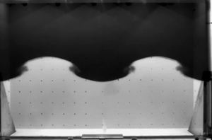
Concerning more specifically the transition to turbulence in the Faraday problem, it is known since Ciliberto & Gollub (Reference Ciliberto and Gollub1985) and Meron (Reference Meron1987) that chaotic behaviours often appear for parameters in the vicinity of the neutral branch intersections of the stability diagram. The experiments presented in Briard et al. (Reference Briard, Gostiaux and Gréa2020) postulate several scenarios of transition to turbulence. For instance, due to the large dimensions of the tank allowing viscous effects to be negligible, harmonic and subharmonic modes can interact to generate mixing at small scales as also reported in numerical simulations (Briard, Gréa & Gostiaux Reference Briard, Gréa and Gostiaux2019). However, this experimental campaign also evidences that turbulence can result from the breaking process of a single Faraday mode. This phenomenon is illustrated in figure 1 (see also supplementary movies available at https://doi.org/10.1017/jfm.2021.1124), showing a growing subharmonic primary Faraday wave subjected to a destabilization process occurring at the nodes and rapidly producing turbulent mixing. The objective of this work is to investigate and explain this mechanism.

Figure 1. The breaking of a Faraday wave in the FARAMIX experiment. (a) Visualization showing the tank geometry and the configuration (also presented in Briard et al. Reference Briard, Gostiaux and Gréa2020). (b) Time series images from the camera zooming on one wavelength and presenting two oscillation periods of the primary wave. This illustrates the different stages of the wavebreaking, with first a ‘blurring’ of the interface at the node followed by a ‘roll-up’. This case corresponds to the b5 experiment whose parameters are detailed in table 1. (c) Visualization of the interface at wavebreaking in the direct numerical simulation DNSd3 (the parameters are given in table 2). The reference frame as well as the acceleration direction are also indicated.
The breaking of Faraday waves at free surfaces is known to appear at the wave crest and leads to the formation of jets (as shown by Jiang, Perlin & Schultz Reference Jiang, Perlin and Schultz1998; Wright, Yon & Pozrikidis Reference Wright, Yon and Pozrikidis2000; Longuet-Higgins Reference Longuet-Higgins2001; Kalinichenko Reference Kalinichenko2009). This comes from the modulation of the primary wave interacting with its first temporal harmonics. More generally, the crests of the waves in the ocean are also subject to destabilization. Due to its importance, this topic is well documented, shedding light on the many instability mechanisms that can develop (Banner & Peregrine Reference Banner and Peregrine1993; Kiger & Duncan Reference Kiger and Duncan2012). Yet the breaking process of free surface waves differs sensitively from the observations reported in figure 1. By contrast, our problem presents very close similarities with the destabilization of standing waves described by Thorpe (Reference Thorpe1968), also in the context of miscible fluids with small density variations. While the primary wave in Thorpe's experiment is generated not by vertical vibrations but by lateral plungers, a vortex is still produced at the wave node as in figure 1. More precisely, several phases can be identified for the instability with a ‘blurring’ of the interface preceding its ‘roll-up’. Kalinichenko (Reference Kalinichenko2005) has also observed and investigated experimentally the breaking process of a Faraday wave between miscible or immiscible fluids. In particular, he reported that the secondary instability starts for wave steepness  $k a \sim 0.4$, with
  $k$ the wavenumber and
  $a$ the amplitude of the Faraday wave. The Rayleigh–Taylor type instability does not seem to play a role in the process as the acceleration induced by the primary wave displacement is not sufficient to invert the gravity. Thorpe (Reference Thorpe1968) and Kalinichenko (Reference Kalinichenko2005) suggest instead that a sort of Kelvin–Helmholtz instability, ‘although not in a simple form’, is at work. Due to the strong time dependence of this configuration, evaluating locally the Richardson number at the node cannot be sufficient to assess the importance of the shear instability. Additionally, in the context of internal gravity waves, the role of subharmonic secondary parametric instabilities in the breaking process has been explored (McEwan & Robinson Reference McEwan and Robinson1975; Bouruet-Aubertot, Sommeria & Staquet Reference Bouruet-Aubertot, Sommeria and Staquet1995; Benielli & Sommeria Reference Benielli and Sommeria1998; Staquet & Sommeria Reference Staquet and Sommeria2002; Sutherland Reference Sutherland2010; Yalim, Lopez & Welfert Reference Yalim, Lopez and Welfert2020). Can this mechanism also apply to Faraday waves?
This paper is organized as follows. We give in § 2 a brief description of the experiments and numerical simulations used for this study. In § 3, we analyse the characteristics of the primary Faraday wave, emphasizing in particular the mode selection mechanism. Section 4 is dedicated to the wavebreaking process, with two theoretical approaches proposed and shedding light on the importance of a subharmonic secondary instability. We then detail our methodology in order to measure the wavebreaking amplitudes in § 5. Finally, the analysis and discussion of the results in view of the theoretical predictions are provided in § 5.3.
2. Generalities
This work, dedicated to the wavebreaking of Faraday waves, relies on several experiments already presented in Briard et al. (Reference Briard, Gostiaux and Gréa2020) and initially designed to study the turbulent mixing driven by vertical vibrations. First, we detail the configuration used and the parameters considered. Next, we present the direct numerical simulations that allow us to explore an even broader range of parameters and to identify how the transition to turbulence takes place.
2.1. Experimental set-up and parameters
The experimental set-up is now introduced briefly since the details can be found in Briard et al. (Reference Briard, Gostiaux and Gréa2020). We fill a cuboidal tank of inner length  $W=94.6 \ \text {cm}$, width
  $D=11 \ \text {cm}$, and height
  $H=67 \ \text {cm}$, with salt and fresh water (see figure 1). The salt water density takes the values
  $\rho _1=1030$,
  $1060$ or
  $1090 \ \text {kg} \ \text {m}^{-3}$, while for the fresh water we get
  $\rho _2=998 \ \text {kg} \ \text {m}^{-3}$. This corresponds to various Atwood numbers expressing the density contrast:
  $\mathcal {A}=(\rho _1-\rho _2)/(\rho _1+\rho _2) \in \{0.015, 0.03, 0.045 \}$. The heavier salt water layer is initially placed at the bottom. It is separated from the lighter fresh water by a thin diffuse interface of thickness
  $\delta =0.5 - 1.5 \ \text {cm}$ located at half the height of the tank. This thickness may vary due to the filling procedure of the tank. The values of
  $\delta$ can be measured either by the initial image from the camera or by the vertical density profiles obtained from a probe before the experiment starts.
A hexapod oscillates the tank along the  $z$ (vertical) direction (for the horizontal directions,
  $x$ corresponds to the length
  $W$, and
  $y$ is along the width
  $D$ of the tank). This generates a well-controlled time-dependent vertical acceleration of intensity
  $G(t)= G_0 (1+ F \cos \omega t)$. Here
  $G_0=9.81\ \text {m}\ \text {s}^{-2}$ is the usual gravitational acceleration,
  $\omega$ is the frequency, and
  $F$ is the forcing parameter. This forcing parameter is related to the vertical displacement amplitude of the hexapod,
  $a_h$, as
  $F= a_h \omega ^{2} /G_0$. In the experiments, the acceleration does not change sign since
  $F <1$, although the displacement amplitude of the vessel can be as large as
  $a_h=45$ cm.
We select in Briard et al. (Reference Briard, Gostiaux and Gréa2020) the experiments with sharp initial interfaces and developing a single Faraday wave. The cases exhibiting different modes appearing simultaneously are not considered. Therefore our study is based on  $18$ experiments shown in table 1, and grouped by values of
  $\mathcal {A}$.
Table 1. Label (series and number), Atwood number, forcing parameter and frequency considered for the experiments in this work. The wavenumbers and mode types corresponding to the primary Faraday wave are also indicated. The initial interface thickness  $\delta$ is measured either by a probe when available or directly from the camera (labelled with
  $*$).
$*$).

The primary standing Faraday waves observed in these experiments are characterized by a horizontal wavenumber,  $k_{m,n}=\sqrt {k_x^{2}+k_y^{2}}$, associated with the mode index in the
  $x$ and
  $y$ directions, respectively,
  $m=k_x W /{\rm \pi}$ and
  $n=k_y D /{\rm \pi}$. So, for instance,
  $m=2$ corresponds to a wavelength equalling the width
  $W$ of the tank. As the primary wave is ‘two-dimensional’, this implies a zero mode index
  $n=0$. It can be seen in table 1 that configurations with odd and even modes have been investigated.
2.2. Direct numerical simulations
In this work, we also provide direct numerical simulations (DNS) in order to explore a broader panel of parameters and to investigate the inner mechanisms of wavebreaking.
These simulations solve numerically the Navier–Stokes equations under the Boussinesq approximation. They express the dynamics of the incompressible fluid velocity  ${{\boldsymbol {U}}} ({{\boldsymbol {x}}},t)$ and the concentration of heavy fluid
  $C({{\boldsymbol {x}}},t)$. Here for miscible fluids with small Atwood number, the dimensionless concentration
  $C({{\boldsymbol {x}}},t) \in [0 \ 1]$ is related to the density as
  $\rho ({{\boldsymbol {x}}},t)= \rho _2+(\rho _1-\rho _2)\,C({{\boldsymbol {x}}},t)$. In the reference frame attached to the container, this leads to the classical system of equations
 $$\begin{gather} \partial _t {{\boldsymbol{U}}}+{{\boldsymbol{U}}} \boldsymbol{\cdot} \boldsymbol{\nabla} {{\boldsymbol{U}}}={-}\boldsymbol{\nabla} \varPi -2 \mathcal{A}\,G (t)\,C {\boldsymbol{e}}_z + \nu\,\nabla ^{2} {{\boldsymbol{U}}}, \end{gather}$$
 $$\begin{gather}\partial _t C +{{\boldsymbol{U}}} \boldsymbol{\cdot} \boldsymbol{\nabla} C=\mathcal{D}\,\nabla ^{2} C, \end{gather}$$
 $$\begin{gather}\boldsymbol{\nabla} \boldsymbol{\cdot} {{\boldsymbol{U}}}=0. \end{gather}$$
 In (2.1a)–(2.1c),  $\varPi$ refers to a reduced pressure, and
  $\nu, \mathcal {D}$ are the kinematic viscosity and molecular diffusion coefficients, respectively. This set of equations constitutes our theoretical framework in order to predict the wavebreaking. It also describes reasonably well the flow dynamics at large scale in the experiments, despite the variations of the viscosity and diffusion coefficients,
  ${<} 20\,\%$, between fresh and salt water.
The simulations are performed in a triply periodic cubic box of size  $W$ (or
  $2 W$) using the code already described in Briard et al. (Reference Briard, Gréa and Gostiaux2019, Reference Briard, Gostiaux and Gréa2020). Therefore we do not seek to reproduce the tank's walls, which do not play a direct role in the wavebreaking phenomenology (although the walls can play a decisive role in the final transition to turbulence). The code is based on a pseudo-spectral collocation method with two-thirds rule dealiasing. The time advancement is realized through a third-order low-storage strong-stability-preserving Runge–Kutta scheme, with implicit viscous terms. All the simulations use a
  $1024^{3}$ grid box with a pencil decomposition on either 1024 or 2048 cores. Due to the vertical periodicity, a thin penalization layer is applied to freeze the velocity and concentration fields at the top and bottom of the computational domain. This method is described extensively in appendix B of Briard et al. (Reference Briard, Gostiaux and Gréa2020). Several tests varying the width of the penalization band have been conducted in order to ensure that this vertical treatment has no impact on the dynamics of the interface. In all the simulations presented, the amplitude of the Faraday wave is less than half of the vertical height of the non-penalized domain.
The simulations parameters are presented in table 2. In order to have a well-resolved flow field, the viscosity and diffusion are fixed at  $\nu =\mathcal {D}=2.26 \times 10^{-6}\ \text {m}^{2}\ \text {s}^{-1}$. This corresponds to roughly twice the real viscosity of water but largely overestimates the molecular diffusion (the Schmidt number is
  $1$ instead of
  $700$ for salt water). Due to the dimensions of the tank, this limitation does not prevent us from properly capturing at least the first stages of secondary instabilities developing on the Faraday wave.
Table 2. Label (series and number) and parameters in physical units (Atwood number, forcing parameter and frequency) taken for the direct numerical simulations presented in this work. The cases DNSa, DNSd and DNSe correspond to the wavebreaking detection. The series DNSb and DNSc are dedicated to the competition between modes  $(2,0)$ and
  $(3,0)$, where the selected mode appears underlined. The parameter
  $r$ expresses the initial amplitude ratio (
 $r=0$ corresponding to a pure
  $(2,0)$ mode). The initial amplitude
  $\epsilon$ of the interface perturbation and the
  $y$-spanwise perturbation amplitude
  $\epsilon _1$ for DNSf, together with the interface thicknesses
  $\delta$, are also detailed. The computation domain is of cubic size with length
  $W=94.6$ cm or
  $2W$ for the series labelled with
  $^{*}$. All the DNS have a
  $1024^{3}$ grid resolution.

We now detail the initial conditions taken in the simulations. While the initial velocity is  ${{\boldsymbol {U}}}=0$ in the simulations, the initial concentration profile is taken as two-dimensional (2-D) of the form (for the DNSa, DNSd and DNSe series and outside the penalization band)
 \begin{equation} C(x,z)=\frac{1}{2} \left ( 1+\text{tanh} \left[ \frac{z-\xi(x)}{\sigma}\right]\right), \quad \text{with} \ \xi(x)=\epsilon \sin (k_{m,0} x). \end{equation}
The parameter  $\sigma$ in (2.2) sets the initial width
  $\delta$ of the interface (
 $\delta \approx 3 \sigma$). The function
  $\xi (x)$ indicates the initial perturbed interface position of sinusoidal shape, with wavelength
  $k$ and of small amplitude
  $\epsilon =1.5$ cm. Therefore the initial interface is slightly more diffused and has a larger amplitude in the simulations compared to the experiments. This is to have at least
  $20$ grid points across the interface layer and to ensure grid convergence of the simulations.
Without ambiguity, the initial wavenumber  $k_{m,0}$ for DNSa, DNSd and DNSe also corresponds to the observed wavenumber at later times indicated in table 2 and characterizing the subharmonic Faraday wave. This is due to our choice for the forcing frequency taken as nearly twice the value of the dispersion relationship of an inviscid interface
  $\omega =2 \sqrt {\mathcal {A} G_0 k_{m,0}}$.
In order to explore more broadly the effect of mode selection, we also propose simulations DNSb and DNSc with an initial interface position defined as
 \begin{equation} \xi(x) = \epsilon [r \cos(k_{3,0} x) + (1-r) \cos(k_{2,0} x)]. \end{equation}
Here, the parameter  $r$ thus expresses the initial ratio amplitude between the modes
  $(3,0)$ and
  $(2,0)$. These simulations are conducted in a computational domain twice the size of the tank,
  $2W$, in order to allow the development of odd modes otherwise forbidden due to the periodic boundary conditions. Also, the interface thicknesses
  $\delta$ are doubled to keep at least 10 grid points across the interface, while the viscosity and diffusion coefficients are still multiplied by
  $4$ to ensure grid convergence of these simulations.
In the simulation series DNSa–DNSe, the flow remains two-dimensional even after the secondary instability starts. In order to study the full transition to turbulence, we consider simulations DNSf where the interface position is slightly perturbed in the spanwise direction  $y$. Introducing the normalized white noise function
  $f$, the interface position is given by
 \begin{equation} \xi(x,y)=\epsilon \sin (k_{m,0} x)+\epsilon_1\,f (y). \end{equation}
In practice, the  $y$ disturbance amplitude is set such that
  $\epsilon _1=10^{-2} \epsilon$. However, we have also tested various simulations varying the
  $\epsilon _1$ parameter, not presented as exhibiting the same phenomenology as DNSf. The breaking of the spanwise symmetry invariance in DNSf can also be produced by the lateral boundary layers in the experiments. Therefore various simulations mimicking the lateral boundary layers were also conducted using the penalization method introduced in Briard et al. (Reference Briard, Gostiaux and Gréa2020). These simulations (not presented) give results similar to those for DNSf, which will be discussed in § 5.3.3.
3. Mode selection mechanism of the Faraday wave
In this section, we discuss the primary wave characteristics and figure out which – linear or nonlinear – mechanism eventually selects the dominant wavelength of the instability in the experiments.
3.1. Linear theory
It is well-known since Benjamin & Ursell (Reference Benjamin and Ursell1954) that when modelling the Faraday instability, the amplitudes,  $\eta _k$, for the interface modes of wavenumber
  $k$ are ruled by a Mathieu equation
 \begin{equation} \ddot{\eta}_k +2\,\gamma(k)\,\dot{\eta}_k +\varOmega ^{2}(k)\,(1+ F \cos \omega t) \eta_k=0. \end{equation}
 In (3.1), we define the inviscid frequency of the diffuse interface  $\varOmega$ and the viscous damping term
  $\gamma$, both of which depend on the horizontal wavenumber
  $k$. Note that the decoupling of each inviscid mode is true only in the limit of small damping. However, the full analysis of this problem can be performed using the method proposed by Kumar & Tuckerman (Reference Kumar and Tuckerman1994).
The inviscid frequency  $\varOmega (k)$ within the deep-water approximation is thus a growing function of
  $k$ and can be evaluated for a given vertical density profile; see, for instance, Briard et al. (Reference Briard, Gostiaux and Gréa2020) for a piecewise linear profile
 \begin{equation} \varOmega (k)=\left( \frac{\mathcal{A} G_0 k}{1+ k \delta/2}\right)^{1/2}. \end{equation}
For small wavenumbers, i.e.  $k \delta \ll 1$ with
  $\delta$ the thickness of the interface, the classical dispersion relationship for an interface within the deep-water approximation
  $\varOmega =\sqrt {\mathcal {A} G_0 k}$ is recovered. In the large wavenumber limit,
  $k \delta \gg 1$, the interface mode reduces to
  $\varOmega (k)=\sqrt {2 \mathcal {A} G_0 /\delta }$, corresponding to the local buoyancy or Brunt–Väisälä frequency at the interface.
The viscous dissipation term,  $\gamma (k)$, expressing the small interfacial mode damping, can have different origins. The damping coming from the bulk flow for a sharp interface takes the form
  $\gamma _b(k)=2 \nu k^{2}$ (Lamb Reference Lamb1945; Landau & Lifshitz Reference Landau and Lifshitz2013). However, due to the velocity gradients, significant damping can also occur within the thin layer separating the two fluids. Assuming a piecewise linear vertical density profile, Briard et al. (Reference Briard, Gostiaux and Gréa2020) obtained the expression
  $\gamma _\delta (k)=\mathcal {A} G_0 \nu k^{2}/ \varOmega ^{2} \delta \approx \nu k/\delta$ for
  $k \delta \ll 1$. In this linear theory, we wish also to account for the damping generated by the boundary layers at the various walls (top, bottom and laterals) existing in the experiments. The boundary layer widths in the experiment can be evaluated using
  $\delta _w=(2 \nu / \varOmega )^{1/2}$. This gives values
  $\delta _w \sim 1 - 2 \ \text {mm}$ using the parameters of the experiments, showing that the boundary layer widths are much smaller than the characteristics wavelengths of the instability and the size of the tank. In this condition, Keulegan (Reference Keulegan1959) and Miles & Benjamin (Reference Miles and Benjamin1967) have derived an expression for the damping of free surface waves in a rectangular basin due to the laminar boundary layers. This result has also been generalized to our problem by Thorpe (Reference Thorpe1968) as detailed in Appendix B, and leads to the following expression for the damping coefficient:
 \begin{equation} \gamma _{w}\approx \frac{\nu}{D \delta_w}= \frac{\sqrt{\nu \varOmega}}{\sqrt{2}D}.\end{equation}
Here, (3.3) thus expresses the dominant contribution of the lateral walls (in the  $z$–
$z$– $x$ plane) to the damping.
We gather in table 3 the numerical values of the damping coefficients originating from the bulk, the interfacial layer separating the fluids, and the boundary layers at the walls. It can be shown that these values do not vary by more than several per cent if we account for the viscosity contrast between fresh and salt water. Therefore it clearly indicates that the dissipation occurs essentially in the viscous layers at the walls, as  $\gamma _w$ is larger than the other contributions. The damping
  $\gamma _{w}$ indeed scales like
  $\nu ^{1/2}$ in (3.3), while it is linear in
  $\nu$ for the dissipation
  $\gamma _b$ or from the interfacial layer
  $\gamma _\delta$. Bechhoefer et al. (Reference Bechhoefer, Ego, Manneville and Johnson1995) have extensively discussed this aspect and they suggest using fluids with high viscosity in order to better control the dissipation in experiments dedicated to the study of the instability threshold. By contrast, our study is focused on the wavebreaking mechanism, explaining why we favour the use of low-viscosity fluids. Note that for larger wavenumber
  $k$, the contributions from the interface layer regain importance and cannot be neglected.
Table 3. Values for the damping coefficients,  $\gamma _w, \gamma _b, \gamma _\delta$, in
  $\text {s}^{-1}$ and evaluated for the largest wavelengths developing in the experiment. We assume here that the Atwood number is
  $\mathcal {A} =0.03$ and the thickness of the interfacial layer is
  $\delta =0.5 \ \text {cm}$. Here, the top boundary is taken as a wall to evaluate
  $\gamma_w$ (the values would be nearly the same for a free surface).

The stability diagram corresponding to the first subharmonic tongue is represented in figure 2. It is plotted for the different large-scale modes of the tank and derived using the damping  $\gamma _w$ from (3.3) and
  $\gamma _\delta$ (the latter contribution being smaller). The neutral curves of (3.1) are computed using the method proposed by Kumar & Tuckerman (Reference Kumar and Tuckerman1994) and also used in Briard et al. (Reference Briard, Gostiaux and Gréa2020) assuming different Atwood number values
  $\mathcal {A}$ and an initial interface thickness
  $\delta =1$ cm. For a given mode
  $k$, the minimum forcing
  $F_{th}$ able to destabilize the interface occurs at the frequency corresponding to the first subharmonic resonance,
  $\varOmega (k) =\omega /2$. The classical asymptotic theory of the Mathieu equation, in the limit of small damping, allows the derivation of the threshold as
  $F_{th}=8 \gamma /\omega$ (see Rajchenbach & Clamond (Reference Rajchenbach and Clamond2015), for instance). The threshold
  $F_{th}$ varies very weakly for the different modes presented in figure 2. Indeed, the contribution due to the damping from the viscous layer at the walls scales like
  $\gamma _w \sim \omega ^{1/2}$, leading to a decrease of
  $F_{th}$ at larger
  $\omega$. However, this effect is compensated at larger
  $k$ by the contribution from the damping at the interface scaling like
  $\gamma _\delta \sim \omega ^{2}$.

Figure 2. Stability diagram for (3.1) in a non-dimensional frequency  $\omega /\sqrt {\mathcal {A} G_0 k_{2,0}}$ and forcing
  $F$ plane. The coloured regions correspond to the first subharmonic instability band associated with the different modes of the tank (the mode number is indicated in the figure). The diagram is obtained using the damping coefficient
  $\gamma =\gamma _\delta +\gamma _w$ at three different Atwood numbers
  $\mathcal {A}$, and considering an interface thickness
  $\delta =1 \ \text {cm}$. The neutral curves (thick plain lines) have a slight dependence on the Atwood number, explaining why they are not completely superimposed. The symbols correspond to the parameters taken in the experiment in table 1. The shapes indicate the Atwood number, and the colours reveal which mode is eventually selected.
The parameters taken in the experiments with  $F\geqslant 0.3$, also indicated in figure 2, are situated in unstable regions well above the viscous thresholds determined by the linear Floquet theory. As a consequence, at least two or more modes can be simultaneously subharmonically unstable in these experiments.
3.2. Linear or nonlinear mode selection?
In this subsection, we investigate the mechanisms leading to the mode selection of the primary wave. As shown in figure 2 and due to the large acceleration forcing  $F$, several modes can be linearly unstable and play a role in the interface dynamics. Surprisingly, a single mode, corresponding nearly always to the smallest unstable wavelength, emerges from this process; there is a clear tendency to favour the modes pertaining to the right unstable tongues in figure 2 (the mode reported in table 1 is also indicated by the colour of the symbol in figure 2). In addition, the selection mechanism does not apparently discriminate between the even and odd modes of the tank as both can be observed in the experiments.
One would expect the modes with the largest linear growth rates to be selected first; this is why only the modes in the first subharmonic band are considered here, as the higher resonance regions exhibit much smaller amplification rates. For a given mode, the Floquet theory shows that the maximum amplification occurs for parameters close to the subharmonic resonance frequency located at the centre of the instability tongue. However, the results in figure 2 reveal that in many cases, the selected mode does not have the largest linear growth rate. Moreover, some of the observed modes are hardly unstable and should have very small growth rate from linear theory (such as EXPa1, for instance). This statement stands even if we account for some experimental uncertainties in term of Atwood number ( ${\pm }0.001$) or initial interface width (
 ${\pm }0.5$ cm). It can be shown that these effects only slightly modify the instability tongues of figure 2. In particular, a larger interface thickness would slightly left-shift the instability tongues of figure 2 as the natural frequencies
  $\varOmega$ are decreased (the damping dominated by the viscous layer at the wall remains unchanged). In any case, we have checked that the hexapod movement is well controlled and remains sinusoidal. Therefore it is unlikely to have spurious forcing frequencies in the system that may change the linear stability of the problem.
The initial perturbation of the interface may also play a role in the mode selection mechanism. A large initial amplitude on a given mode can explain why it appears even if it does not have the largest growth rate during the linear phase. This would suggest that an initial condition at small scales is at work in the experiments, although we have not observed such a disturbance and could not identify a source able to generate it. In any case, this cannot shed light on the appearance of linearly stable modes.
By contrast, Faraday experiments with immiscible fluids have revealed the ability of nonlinearities to select modes and generate transient chaotic regimes (see, for instance, Ciliberto & Gollub Reference Ciliberto and Gollub1984, Reference Ciliberto and Gollub1985). Using weakly nonlinear approaches, Meron & Procaccia (Reference Meron and Procaccia1986) and Meron (Reference Meron1987) have already detailed how the mode suppression phenomenon can occur. Considering two modes close to the first subharmonic resonance, the nonlinear cubic coupling terms in each amplitude equation have a sign determined by the detuning parameter  $\varDelta ={\varOmega ^{2}}/{\omega ^{2}}-{1}/{4}$. Here, the detuning parameter for a given mode expresses the departure of the forcing frequency from the first subharmonic resonance. Therefore, when two modes are in competition, their respective detuning parameters
  $\varDelta$ generally have opposite signs because the forcing frequency
  $\omega$ lies between the two subharmonic resonance frequencies (see figure 2). This explains the mode suppression since one mode can develop, even being linearly stable, by pumping energy from the other one. The theory indeed shows that the vanishing mode,
  $\varDelta < 0$, is supercritical as the nonlinear coupling damps the instability while the dominant one,
  $\varDelta \geqslant 0$, is subcritical as it is being reinforced by the nonlinearities. As the wave amplitude grows, the frequency of the wave tends to diminish (Thorpe Reference Thorpe1968) as well as the detuning parameter of each mode (Godrèche & Manneville Reference Godrèche and Manneville2005). Hence this left-shifts the instability bands of figure 2 and favours the subcritical modes at smaller wavelength.
3.3. Numerical analysis of the mode competition
At this stage, the mode suppression due to a nonlinear coupling between competing modes can explain the mode selection evidenced in figure 2. In any case, the mode amplitude is no longer negligible compared to its wavelength when the selection process is at work, suggesting that the nonlinear effects are an important ingredient to account for. We wish to assess further this hypothesis by the mean of direct numerical simulations (DNS) with well-characterized initial conditions. Two series of DNS have been performed using  $1024^{3}$ grid points (series DNSb and DNSc in table 2), with
  $\mathcal {A} =0.03$. The frequency
  $\omega$ and the forcing
  $F$ taken in the simulations are also represented in the phase diagram of figure 3. It is important to stress here that the phase diagram does not account for the wall damping as simulations are performed in a triply periodic box. The two series of DNS start from the same location in the phase diagram (point
  $A$) with
  $F=0.8$ and
  $\omega =3.07$ (or equivalently
  $\omega / \sqrt { \mathcal {A} G_0 k_{2,0}}=2.2$). This corresponds to parameters with the two unstable modes having nearly the same exponential growth rate as
  $\sim {\rm e}^{\lambda \omega t}$. Indeed, the Floquet exponent
  $\lambda$ takes the value
  $0.09$ for mode
  $(3,0)$, and
  $0.07$ for mode
  $(2,0)$. We fix the forcing parameters in one series and vary the amplitude ratio
  $r$. In the other series, the relative amplitude is set at
  $r=0.5$ and we decrease the forcing frequency
  $\omega$ in order to explore more deeply the
  $(2,0)$ subharmonic instability tongue. The simulations are stopped when the wavebreaking occurs and we report which of the
  $(2,0)$ and
  $(3,0)$ modes prevails at this moment in figure 3. This procedure is performed both visually and by computing the Fourier modes of the interface.

Figure 3. Parameters of the DNS (symbols) in the stability diagram  $\omega$–
 $F$. The coloured areas correspond to the subharmonic instability tongues for the modes
  $(2,0)$ and
  $(3,0)$ accounting for viscosity and diffused interface
  $\delta =1.8 \ \text {cm}$ (as no walls are present in the DNS, the damping coefficient
  $\gamma \approx \gamma _\delta$ and critical thresholds
  $F_{th}$ are very small). The symbols’ colours indicate which mode emerges from the simulation; mixed colours express that both modes can be observed. Two series of DNSb, DNSc (see table 2) are presented here, starting from point
  $A$. In the DNSb group, the initial amplitude ratio
  $r$ between modes
  $(3,0)$ and
  $(2,0)$ is set at
  $r=0.5$ and we decrease the forcing frequency
  $\omega$. In the DNSc group, the frequency and forcing are fixed and we vary
  $r$. The point corresponding to DNSe is also placed.
The simulations clearly evidence the mode suppression phenomenon to the benefit of the modes with the smallest wavelength. The results reported in figure 3 show the dominance of mode  $(3,0)$ even starting from a small initial amplitude (transition occurs at
  $r=0.1$) or developing in a region where it is linearly stable (for small
  $\omega$). The phenomenon can be scrutinized in more detail in the snapshots extracted from the two series in figure 4, where the mode
  $(3,0)$ emerges from cases with initial
  $r=0.25, \ 0.5$ or with the frequencies
  $\omega =2.6, \ 2.8$. Indeed, in the last row of figure 4, one can observe that mode
  $(2,0)$ prevails only for
  $\omega =2.4$ (
 $\omega /\sqrt {\mathcal {A} G_0 k_{2,0}}=1.72$), and for larger
  $\omega$, say
  $\omega =2.6$ (or
  $\omega /\sqrt {\mathcal {A} G_0 k_{2,0}}=1.86$), mode
  $(3,0)$ is visible despite being linearly stable. As a consequence, the mode competition greatly enhances the sensitivity to initial conditions in the experiment. As importantly, this process breaks the symmetry of the primary wave, as can be seen in both the experiments (figure 1) and the simulations (figure 4).

Figure 4. Mode selection in six DNS of figure 3. (a) Cases corresponding to DNSc (see table 2) with  $r$ varying and
  $\mathcal {A}=0.030$,
  $\omega =3.07$,
  $F=0.8$. The amplitude of the interface deformation is
  $\epsilon =3 \ \text {cm}$. (b) Cases corresponding to DNSb (see table 2) with
  $\omega$ varying and
  $\mathcal {A}=0.030$,
  $F=0.8$,
  $r=0.5$,
  $\epsilon =1.5 \ \text {cm}$. We put the slices of width
  $W$ of the concentration field at four instants starting from the initial interface at
  $t=0$ and ending when the wavebreaking occurs; pure fluids remain in white, while mixed fluid with
  $C = 0.5 \pm 0.15$ is in black.
Some specificities of the mode suppression in our Faraday experiment with miscible fluids are now addressed. We have not observed oscillations between two specific modes as in Ciliberto & Gollub (Reference Ciliberto and Gollub1984, Reference Ciliberto and Gollub1985) or similarly Yalim, Welfert & Lopez (Reference Yalim, Welfert and Lopez2019) in the context of a stable stratification. This is notably because, at large forcing parameter, the interface grows irreversibly, allowing continuously new modes to be destabilized. The modes can change in our experiment, as already reported in Briard et al. (Reference Briard, Gostiaux and Gréa2020). But there is always a correspondence to a one-way transition from large to small wavelength for interface modes. The more complex transitions evidenced in figure 14 of Briard et al. (Reference Briard, Gostiaux and Gréa2020), for instance, refer to modes not pertaining to the same instability band or being of different natures. The irreversible mixing produced by the rapid breaking of the primary waves also explains this aspect.
Another difference with past Faraday immiscible experiments conducted in a shallow basin is that in our case the dominant waves correspond to those with the smallest wavelength, as already discussed. Noticeably, this point clearly agrees with the nonlinear theory of mode suppression. It can be shown that within the deep-water approximation, the subcritical modes are indeed those with small wavelength; see Rajchenbach & Clamond (Reference Rajchenbach and Clamond2015) for details.
In this section, it has been evidenced that the mode selection of the primary wave may result from a complex nonlinear mode competition process. When this is the case, the subcritical mode is eventually selected. In the following, we try to explain the breakdown of the Faraday waves.
4. Modelling the breakdown of Faraday waves
We now present two heuristic models dedicated to the breakdown of Faraday waves initiating the transition to turbulent mixing. The objective is to evaluate the critical wave steepness at which the breakdown may occur. By emphasizing two simple approaches, we aim to explore various frameworks for the breakdown and to disentangle the inner mechanisms responsible for the instability.
Both models, although relying on different assumptions, suggest that the breakdown results from a subharmonic secondary instability at small scales. Therefore one key ingredient in these approaches is to account for the unsteadiness of the primary wave. This aspect differs from secondary instability analysis relying on a frozen base flow used, for instance, in the context of Kelvin–Helmholtz instability (Salehipour, Peltier & Mashayek Reference Salehipour, Peltier and Mashayek2015).
The first approach, hereafter referred as global, is based on the fact that the breakdown of the Faraday waves changes the monotony of horizontally averaged density profiles (this point is more specifically detailed later, in § 5.2). We therefore seek to identify the conditions for a small disturbance to develop around the mean profile characterizing a Faraday wave of given amplitude (see figure 5). By contrast, the second model proposed relies on the local analysis of small perturbations at the interface node of the primary wave (see also figure 5).

Figure 5. Frameworks applied to model the wavebreaking of the primary wave (a) and detailed in § 4. For the global approach (b), we consider the stability of the horizontally averaged concentration profiles. For the local approach (c), we study the development of small perturbations of wavenumber  $k_{wb}$ at the node of the primary wave.
4.1. The global approach
4.1.1. A simple model equation
In order to derive a simple model for the breakdown of Faraday waves, the concentration and velocity fields are decomposed into a mean and a fluctuating part as  $C=\bar {C} +c$ and
  ${\boldsymbol {U}}=\bar {{\boldsymbol {U}}} +{\boldsymbol {u}}$. A mean quantity
  $\bar {*}$ is obtained by averaging along the horizontal
  $x$ and
  $y$ directions. The system (2.1) is classically averaged also in order to find the equations for the mean flow and its fluctuations. It can be shown directly that the mean velocity is zero,
  $\bar {\boldsymbol {U}}=0$, due to the symmetries and the incompressibility condition. The mean vertical concentration profile
  $\bar {C} (z,t)$ evolves principally due to the vertical buoyancy flux
  $\overline {w c}$ as
 \begin{equation} \partial_t \bar{C}+ \partial_z \overline{w c}=\mathcal{D} \partial^{2} _{zz} \bar{C}.\end{equation}
In this global approach, the primary Faraday wave is thus embedded in the mean vertical concentration profile  $\bar {C} (z,t)$ but also has fluctuation components satisfying (4.1).
Further simplifications are now made in order to obtain a more tractable model. We seek a ‘rapid’ secondary instability occurring at small scales and located at  $z=0$. In this context, the rapid acceleration theory initially developed by Hunt & Carruthers (Reference Hunt and Carruthers1990) and applied to turbulent mixing layers in Gréa (Reference Gréa2013) provides a convenient framework for expressing the dynamics of small-scale disturbances. We thus discard all the dissipative and nonlinear terms, except for the coupling between the fluctuations and the mean concentration field. In addition, the small-scale disturbance sees only a uniform mean concentration gradient at
  $z=0$ determined by the length
  $L=-1/\partial _z \bar {C}(0,t)$. Within this quasi-homogeneous approximation, the small-scale fluctuating quantities and pressure
  $p$ are determined by
 $$\begin{gather} \partial _t {\boldsymbol{u}} ={-}\boldsymbol{\nabla} p -2 \mathcal{A}\,G(t)\,c {\boldsymbol{e}}_z, \end{gather}$$
 $$\begin{gather}\partial _t c =\frac{w}{L(t)}, \end{gather}$$
 $$\begin{gather}\boldsymbol{\nabla} \boldsymbol{\cdot} {\boldsymbol{u}}=0. \end{gather}$$
 One recognizes in (4.2) the classical equations for an internal gravity wave, except that it is driven by a time-varying acceleration and mean density gradient. When it is uniform across the layer, this mean gradient can be evaluated from the mixing layer length  $L_{int}= 6 \int _{-\infty } ^{+\infty } \bar {C} (1-\bar {C})\,{\rm d}z$ introduced by Andrews & Spalding (Reference Andrews and Spalding1990) and previously used in Briard et al. (Reference Briard, Gostiaux and Gréa2020) for the fully turbulent regime. However, this property is lost when the flow takes the form of a single laminar wave. In this case, the inverse concentration gradient is maximum at
  $z=0$, and we will discuss in a later section different ways to evaluate it.
These waves depend on their orientations, but for this heuristic model we focus only on waves with a wavevector in the horizontal plane. Differently oriented modes are thought to be less relevant in the secondary instability partly because they are less likely to modify the mean concentration profile; the feedback of the fluctuations to the mean concentration profile is indeed controlled by the vertical buoyancy flux term  $\overline {w c}$, which is weaker for vertically oriented modes. Eliminating
  $w$ in (4.2), we obtain the following Mathieu-like equation (see a more detailed derivation in Gréa & Ebo Adou Reference Gréa and Ebo Adou2018):
 \begin{equation} \ddot{c} + \frac{\dot{L}}{L}\,\dot{c} +\frac{2 \mathcal{A}\,G(t)}{L}\,c=0. \end{equation}
 The concentration fluctuations  $c$ are therefore fully determined by
  $L$, expressing the amplitude of the primary Faraday wave. We need to determine the condition on
  $L$ for which the perturbations may develop. Indeed, the rise of the perturbation foreshadows the breaking process of the primary wave and the onset of turbulence. More precisely, (4.3) exhibits the buoyancy frequency defined as
  $\varOmega _B=(2 \mathcal {A} G_0/L)^{1/2}$ and a damping term
  $\dot {L}/L$ expressing the variations of
  $\varOmega _B$ as the mixing zone width
  $L$ evolves. As will be seen in § 4.2, the
  $\varOmega _B$ frequency is relevant for the secondary instability because the shear at the nodes of the primary wave is driven directly by the wave amplitude.
We now detail the implications of this model equation regarding the wavebreaking phenomenology as observed in figure 1.
4.1.2. The subcritical nature and the criterion for the wavebreaking
The stability of the model equation (4.3) has been extensively discussed in Gréa & Ebo Adou (Reference Gréa and Ebo Adou2018) and Briard et al. (Reference Briard, Gostiaux and Gréa2020), allowing the prediction of the final widths of the turbulent mixing zones. This saturation criterion evaluates when the subharmonic instability stops, or equivalently when the inner frequencies of the layer are no longer in resonance with the forcing. Thus it did not seek to account for the unsteadiness of  $L$. Conversely, we wish to interpret the wavebreaking as the development of a secondary subharmonic instability at small scales. For a small disturbance characterized by the buoyancy frequency
  $\varOmega _B$, we thus aim to find when it becomes parametrically unstable as the result of both the forcing and the primary wave oscillations. The enlargement of the primary wave amplitude determines not only the instability threshold, but also the later amplification of the secondary instability growth rate. This explains why the secondary instability develops rapidly at the interface, and sheds light on the subcritical nature of this secondary instability. This peculiarity is indeed well-known for nonlinear Mathieu systems such as (4.3) as detailed in Soliman & Thompson (Reference Soliman and Thompson1992) or Godrèche & Manneville (Reference Godrèche and Manneville2005).
In order to derive an analytic criterion for the wavebreaking, we consider the inverse mean concentration gradient  $L$ having the simple form
  $L(t)=L_0 (1+\beta \cos (\omega t))$. The length
  $L$ is thus expected to be proportional to the amplitude
  $\eta _p$ of the primary Faraday wave,
  $L(t) \sim |\eta _p |$ in the laminar phase. Here, the proportionality coefficient depends on the shape of the nonlinear primary wave. Also, the parameter
  $\beta$ expresses the relative amplitude of the Faraday wave oscillations while
  $L_0$ is the mean over one oscillation period. This expression does not account for the primary mode growth, which is assumed small over an oscillation period. It also expresses that for a subharmonic instability,
  $L$ oscillates at frequency
  $\omega$ while
  $\eta _p$ oscillates at frequency
  $\omega /2$. However, the higher temporal harmonics of
  $L(t)$ or
  $\eta _p$ for the primary wave are discarded. In addition, it is important to note that the primary Faraday mode amplitude is in phase with the acceleration
  $G(t)$.
In this context, we use the Floquet analysis detailed in Appendix B to find the secondary subharmonic instability onset. The results are represented in the stability diagram of figure 6, exhibiting the instability tongues for  $\beta =0$ and
  $\beta =0.7$. Note that the case
  $\beta =0$ indeed corresponds to the classical stability diagram of a Mathieu equation. In this representation, the right-hand sides of the neutral branches (solid black lines of figure 6) determine the critical amplitude of the primary wave and the beginning of the secondary instability as
  $L_0$ grows. This gives a critical threshold
  $L_{crit}$ that should be close to the one characterizing the wavebreaking
  $L_{wb}$ if the instability develops quickly (we still have
  $L_{crit}\leqslant L_{wb}$).

Figure 6. Stability analysis of (4.3) with  $L(t)=L_0 (1+\beta \cos (\omega t))$ and represented in the
  $\varOmega _{0B}^{2}/\omega ^{2}$–
 $F$ plane (with
  $\varOmega _{0B}=(2 \mathcal {A} G_0/L_0)^{1/2}$). The two coloured areas indicate the first subharmonic tongues with
  $\beta =0$ and
  $\beta =0.7$, respectively. The dashed blue lines correspond to the approximation (4.4), while the red dashed dotted lines correspond to (B9).
An analytical approximation for the critical threshold  $L_{crit}$ is also derived in Appendix B, leading to
 \begin{equation} L_{crit}\approx\frac{(4-2 F)}{1 +\beta/2}\,\frac{2 \mathcal{A} G_0 }{\omega ^{2}}, \quad \text{for} \ F \ll 1 \ \text{and} \ \beta \ll 1. \end{equation}
As shown in figure 6 (blue dashed lines), the criterion (4.4) slightly underestimates  $L_\text {crit}$ at small
  $F$ and large
  $\beta$ while being reasonably correct for the parameters taken in the experiment. However, it becomes very bad at large
  $F$, even leading to negative values for
  $F \geqslant 2$. Despite being more complicated, a better approximation can be derived corresponding to (B9) and shown by the red dashed dotted lines of figure 6.
In (4.4), we see that the forcing  $F$ together with the movement of the primary wave characterized by
  $\beta$ contribute to the destabilization of the primary wave. In particular, even without acceleration forcing (
 $F=0$), the secondary instability can be triggered by the primary wave oscillations. This also leads to striking differences in terms of growth rates. For instance, for the subharmonic resonance at
  $F=0.7$ we find a Floquet exponent
  $\lambda =0.09$ for
  $\beta =0$ (also corresponding to the growth of the primary wave), while
  $\lambda =0.2$ for the case with
  $\beta =0.7$. Therefore the acceleration induced by the primary wave increases sensibly (but not drastically) the growth rate of the secondary modes. This effect explains why the breakdown occurs in a time scale much shorter than the growth of the primary wave.
4.2. The local approach
The previous global approach has the main advantage of being relatively simple through relying on the horizontal averaging process. The drawback, however, is losing track of the physical mechanism responsible for the secondary instability. Also, it assumes that the secondary instability mode results only from the interaction with the mean component of the primary wave. This assumption may appear excessive, and it motivates us to propose a complementary method. We therefore perform a stability analysis of the flow generated at the node of the primary wave.
The equations driving the evolution of an interfacial perturbation amplitude,  $\eta$, at the node of the primary wave, are given in the inviscid limit (see the derivation in Appendix C) by
 \begin{equation} \ddot{\eta} -2 {\rm i} \mathcal{A} {k_{wb}}U \dot{\eta}+( \mathcal{A}\,G (t)\,{k_{wb}} - {k_{wb}} ^{2} U^{2}-{\rm i} \mathcal{A} {k_{wb}} \dot{U} ) \eta=0. \end{equation}
In (4.5),  ${k_{wb}}$ represents the wavevector modulus of the perturbation, and
  $U$ is the oscillating tangential velocity induced by the primary wave at the node. Not surprisingly, we recover the equation in the Boussinesq limit first derived by Kelly (Reference Kelly1965), expressing the dynamics of an oscillating sheared interface. In fact, supposing the instability amplitude and wavelength are small, respectively
  $k \eta \ll 1$ and
  $\kappa ={k_{wb}}/k \gg 1$, this allows us to neglect the interface tilting at the node and to assume the quasi-homogeneity of the perturbation. Note that often at least two vortices may appear in the experiments at the node of the primary wave during the breaking process, suggesting the validity of the homogeneity assumption.
Many works have been dedicated to the stability analysis of (4.5) in the case of  $G$ constant and
  $U$ oscillating at a single frequency
  $\omega$. In addition to the parametric resonance modes that Kelly (Reference Kelly1965) identified, Lyubimov & Cherepanov (Reference Lyubimov and Cherepanov1987) and Khenner et al. (Reference Khenner, Lyubimov, Belozerova and Roux1999) have shown and derived a criterion for the existence of Kelvin–Helmholtz type modes at the interface. These latter modes generate a longwave instability observed in most experiments, which may exhibit frozen wave patterns at high forcing frequency (Wolf Reference Wolf1970; Wunenburger et al. Reference Wunenburger, Evesque, Chabot, Garrabos, Fauve and Beysens1999; Yoshikawa & Wesfreid Reference Yoshikawa and Wesfreid2011; Gaponenko et al. Reference Gaponenko, Torregrosa, Yasnou, Mialdun and Shevtsova2015; Lyubimov et al. Reference Lyubimov, Khilko, Ivantsov and Lyubimova2017; Gréa & Briard Reference Gréa and Briard2019). Noticeably, frozen waves are completely steady structures analogous to the inclined equilibrium positions of a strongly and horizontally oscillated pendulum.
The local analysis emphasizes the importance of the shear in the breakdown process of the primary wave. Although the works of Thorpe (Reference Thorpe1968) and Kalinichenko (Reference Kalinichenko2005) have early recognized this aspect, the nature of the instability – either Kelvin–Helmholtz (KH) or parametric resonance (PR) type – has not been fully identified in this Faraday wave context. The results of Kelly (Reference Kelly1965) and Khenner et al. (Reference Khenner, Lyubimov, Belozerova and Roux1999) do not apply to our specific configuration where the acceleration oscillates at frequency  $\omega$ while the shear velocity is subharmonic with frequency
  $\omega /2$. We thus reconsider the problem of (4.5) by taking a primary wave of the form
  $\eta _p(t)=a \cos (\omega t/2)$ leading to
 \begin{align} U(t)={-} \frac{\omega a}{2} \sin (\omega t /2)\quad\text{and} \quad U^{2}=\frac{\omega^{2} a^{2}}{8}\,(1-\cos \omega t)= \frac{1}{2}\,\frac{\mathcal{A} G_0 k}{1+ 4 \varDelta}\,a^{2}(1-\cos \omega t), \end{align}
where in the last expression, the subharmonic resonance condition  $\omega ^{2}=4 \mathcal {A} G_0 k/ (1+4 \varDelta )$ for an inviscid interface is used. In order to study the stability of (4.5), it is further convenient to introduce the new variable
  $Y$ defined as
  $\eta = Y \exp ({\int _0^{t} {\rm i} \mathcal {A}{k_{wb}}\,U(t') \,{\rm d} t'})$ giving (at leading order in
  $\mathcal {A}$)
 \begin{equation} \ddot{Y}+( \mathcal{A}\,G(t)\,{k_{wb}} - {k_{wb}} ^{2} U^{2} )Y=0. \end{equation}
Due to the change of variable expression and the fact that  $U$ oscillates at
  $\omega /2$, the response in
  $\eta$ will be also subharmonic. However, for small Atwood number,
  $\eta \approx Y$ and the response can be also nearly synchronous. Indeed, by substituting the expression for
  $U(t)$ into (4.7), we obtain a simple Mathieu equation of the form
 \begin{gather}
\left.\begin{gathered} \ddot{Y}+\left( P +Q \cos (\omega t)
\right) Y =0, \\ \text{with} \ P=\mathcal{A} G_0 k \left(
\kappa -\frac{1}{2(1+ 4 \varDelta)}\,\kappa^{2} (k a)^{2}
\right) \ \text{and} \\
Q=\mathcal{A} G_0 k \left( \kappa F+
\frac{1}{2 (1+ 4 \varDelta)}\,\kappa^{2} (k a)^{2} \right).
\end{gathered}\right\}
\end{gather}
\begin{gather}
\left.\begin{gathered} \ddot{Y}+\left( P +Q \cos (\omega t)
\right) Y =0, \\ \text{with} \ P=\mathcal{A} G_0 k \left(
\kappa -\frac{1}{2(1+ 4 \varDelta)}\,\kappa^{2} (k a)^{2}
\right) \ \text{and} \\
Q=\mathcal{A} G_0 k \left( \kappa F+
\frac{1}{2 (1+ 4 \varDelta)}\,\kappa^{2} (k a)^{2} \right).
\end{gathered}\right\}
\end{gather} In figure 7, we show the stability diagram of (4.8) in a  $\kappa$–
 $k a$ plane (the subharmonic resonance condition for the primary wave is used again). The instability tongue corresponding to the KH type modes appears for
  $P \leqslant 0$, which stands as the classical criterion for the inviscid KH instability,
  ${k_{wb}} \overline { U^{2}} \geqslant \mathcal {A} G_0$ (Chandrasekhar Reference Chandrasekhar1961). The parametric resonance zones start for
  $P \geqslant 0$ but also have a continuation in the opposite half-plane. Remarkably, the instability zones exhibit a very weak dependence on
  $\kappa$ for
  $\kappa \gg 1$. Therefore, at given
  $\kappa$ and as the primary wave amplitude grows, the perturbation passes through the successive instability zones, first the PR types then later the KH one. The growth rates can be computed with the Floquet exponent and show a maximum approximately in the middle of each zone. The KH and PR1 growth rates are larger compared to the other instability zones. Therefore the breakdown of the Faraday wave is expected to occur when the wave steepness,
  $k a$, lies in the instability KH or PR1 zones. This local theory is inviscid, which explains why the growth rates are higher at large
  $\kappa$. Of course, the viscosity and the thickness
  $\delta$ of the interface should play a role and moderate this aspect.

Figure 7. Stability curve of (4.8) for  $F=0.7$ and
  $\varDelta =0$ in the
  $\kappa$–
 $k a$ plane or the
  $P$–
$P$– $Q$ plane (insert) corresponding to the classical representation of the Mathieu equation. The blue coloured areas show the Kelvin–Helmholtz (KH) and parametric resonance (PR) instability regions. The dashed curve corresponds to
  $P=0$. The area corresponding to
  $P<0$ is located above the dashed curve in the
  $\kappa$–
 $k a$ representation. The critical wave steepness value indicated by the black dotted curve corresponds to criterion (4.9).
Similarly to the global approach, we can propose an approximation for the critical wave steepness corresponding to the onset of the PR1 instability. Using the asymptotic expression for the neutral curves of the Mathieu equation in the limit  $P \rightarrow -\infty$,
  $Q \rightarrow +\infty$ detailed in Abramowitz & Stegun (Reference Abramowitz and Stegun1965), we obtain
 \begin{equation} k a _{crit}\approx \tfrac{1}{3} (1+4 \varDelta) (1+F). \end{equation}
This simple expression (4.9) corresponds indeed to the plateau (it does not depend on  $\kappa$) separating the PR1 and PR2 bands in the small perturbation wavelength limit
  $\kappa \gg 1$ as shown in figure 7 (black dotted line).
At this stage, two theoretical approaches have been proposed to study the breaking process of Faraday waves. Before assessing the validity of these approaches, it is first necessary to detail how we detect the wavebreaking in both the experiments and the simulations.
5. Data analysis of the experiments and simulations
In this section, we detail the methodology used in order to measure the primary wave amplitudes and the inverse mean density gradients. We then investigate various strategies to detect the instants at which the wavebreaking occurs. In the last subsection we discuss the validity of the global and local wavebreaking theories against the data from the experiments and DNS.
5.1. Primary wave amplitude and inverse mean density gradient
The global and local approaches detailed in § 4 rely on different scales characterizing the primary wave. These correspond respectively to the inverse mean concentration gradient  $L(t)$ at the rest interface position
  $z=0$ and the wave amplitude
  $\eta _p(t)$ (see also figure 5). It is therefore important to link these two quantities in order to compare the global and local theories in the experiments. As already remarked, we can expect the proportionality between the inverse mean gradient and the wave amplitude,
  $L(t) = \kappa_L |\eta _p (t)|$. This assumes that the shape of the primary wave is frozen, which also determines the coefficient
  $\kappa$. By considering the position
  $\xi _p(x,t)=\eta _p (t) \sin k x$ of a sharp sinusoidal interface, as for the standing wave in Appendix C, we can easily show that
  $\kappa_L = {\rm \pi}$ (the wave amplitude is supposed larger than the interface thickness
  $\delta$). This choice is also motivated by the expression for the finite amplitude standing wave profile given by Thorpe (Reference Thorpe1968) in deep-water approximation, showing that the higher-order corrections are negligible even at moderate wave steepness.
The global theory assumes an inverse density gradient oscillating as  $L(t)=L_0 (1+ \beta \cos \omega t)$, while in the local theory the primary wave amplitude evolves as
  $\eta _p= a \cos \omega t /2$. By expanding
  $|\eta _p (t)|$ in Fourier series and truncating at leading order, we simply get
  $L_0=2 \kappa_L a/{\rm \pi}$ and
  $\beta =2/3$. This allows us to express the results from the global theory in terms of critical steepness, as for the local theory. In particular, the critical wave steepness for the global theory expressed by (4.4) in the limit of small
  $F$, using the resonance condition and taking
  $\kappa_L ={\rm \pi}$ (sinusoidal interface), gives
 \begin{equation} k a_{crit}=\tfrac{3}{8} (2-F)(1+4 \varDelta). \end{equation}
 We now detail how to measure the inverse local gradient  $L$ and the wave amplitude
  $\eta _p$ in practice in the experiments. The inverse local gradient is a difficult quantity to obtain directly from the mean concentration profile. The latter, resulting from the post-processing of the images of the camera as detailed in Briard et al. (Reference Briard, Gostiaux and Gréa2020), can be a bit noisy, particularly when the secondary instabilities start at the node. The quantity
  $|\eta _p|$ can be obtained either from the crest-to-crest amplitude of the wave on the raw camera images, or from an arbitrary threshold on the mean concentration (here taking the height where
  $0.1 \leqslant \bar {C} \leqslant 0.9$). Again this method suffers from being sensitive to small variations in the mean concentration profile. Therefore we find it more convenient to measure these quantities indirectly using the integral length
  $L_{int}$ previously introduced in § 4.1.1. By assuming that the shape of the concentration profiles is frozen, we can deduce all the characteristic lengths from
  $L_{int}$, which for a sinusoidal interface gives
  $L_{int} = 2.4|\eta _p|=0.76 L$.
To ensure that these relations apply in our problem, we have measured the amplitude  $|\eta _p|$ at a local maximum just before the wavebreaking using the threshold method on
  $\bar {C}$, the inverse mean concentration gradient
  $L$, and the integral length
  $L_{int}$. In figures 8(a) and 8(b), we see that the sinusoidal profile is a good fit for the interface position and provides a good evaluation of the mean concentration profile. If the amplitude is too small, however, the fit is less satisfactory, probably because the interface thickness should be accounted for in the evaluation of the mean concentration profile. The method shows that the inverse mean concentration gradient is maximum at the centre of the layer
  $z=0$, in accordance with the fact that the wavebreaking starts at the nodes of the primary wave. In any case, we recover the expected relation between
  $L$ and the wave amplitude
  $|\eta _p|$. Therefore the different lengths
  $L$ and
  $|\eta _p|$ can be evaluated correctly from
  $L_{int}$. In figure 8(c), we further check that the relation between
  $L_{int}$ and
  $|\eta _p|$ holds on multiple experimental data before but close to the wavebreaking. The correlation is thus satisfactory and gives us confidence in our method to extract the amplitudes and the inverse concentration gradients necessary to explore the wavebreaking phenomenon.

Figure 8. (a) Visualization of the interface in experiment EXPa7 (see table 1) at the amplitude maximum just before the wavebreaking and compared to a sinusoidal profile (red line). (b) Mean concentration profile from experiment and sinusoidal interface. (c)  $L_{int}$ plots as a function of
  $|\eta _p|$ at a maximum amplitude just before the wavebreaking for all the experiments of table 1. The values for
  $|\eta _p|$ are evaluated from the crest-to-crest distance of the wave measured directly on the images or using the mean concentration profiles. The two arrows correspond to the EXPa7 case shown in (a,b).
5.2. Wavebreaking detection
In this subsection, we detail the strategy in order to identify the instants corresponding to the wavebreaking in the experiments and the simulations.
The wavebreaking phenomenon can be defined as a local overturning of the interface at the node. This can be observed directly in the images from the camera by noticing the appearance of vortices giving birth to a mushroom-like structure (see figure 9). Since this visual criterion is somewhat subjective, we also propose an automated detection procedure using a simple algorithm based on the Thorpe displacement (introduced by Thorpe Reference Thorpe1977). Indeed, this displacement characterizes the distance that a parcel of fluid has to move vertically in order to be in stable equilibrium with the surrounding water. Hence a completely stable profile would have zero displacements, whereas the existence of some local overturns generates non-zero Thorpe displacements. Accordingly, we compute for each one-dimensional vertical transect the displacements  $\delta _{T} = z^{*}-z$, where
  $z$ is the position of a fluid parcel on the instantaneous concentration field, and
  $z^{*}$ is the position of the same parcel on the vertically sorted concentration field (see figure 9). We detect when this displacement
  $|\delta _{T}|$ exceeds a certain threshold (here
  $|\delta _{T}| > 5 - 12 \textrm {px} = 5.5 - 13.2$ mm) chosen a bit smaller than the initial interface widths. For a given experiment, this algorithm provides almost the same image (and thus same time and value for
  $L$) as the one chosen by eye only (see figure 9). However, it is not possible to detect from this method the beginning of the ‘blurred’ region as defined in Thorpe (Reference Thorpe1968), indicating the secondary instability onset leading to the wavebreaking at the nodes.

Figure 9. Procedure for the wavebreaking detection. (a) Visual criterion from the calibrated camera image. (b) The Thorpe displacements  $\delta _T$ evaluated by sorting the concentration field in each vertical transect of the calibrated image. The colourbar indicates the displacement in mm.
The Thorpe displacement can also be used to measure the vortex size at wavebreaking and thus gives the ratio  $\kappa = {k_{wb}}/ k$ necessary for the local theory. To determine
  ${k_{wb}}$, we take the maximum displacement
  $\delta _{T}$ evaluated at the image given by the Thorpe displacement method. By construction, this measurement cannot be smaller than the arbitrary threshold chosen for the wavebreaking detection. In practice,
  $\delta _{T}$ exceeds this value by more than three times. As a summary, we illustrate in figure 10 the whole procedure allowing for the wavebreaking detection and the measurements of the wave amplitudes and inverse concentration gradients.

Figure 10. Time evolution of the mixing zone width and the mean concentration profiles at different instants extracted from DNSd2 (see parameters in table 2). (a) Evolution of the integral lengths  $L_{int}$ and
  $L_{int,s}$ computed from the mean and sorted concentration profiles, respectively, as a function of
  $\omega t$. The green dotted line corresponds to the integral scale
  $L_{int,d}$ expressing the thickening of the interface by diffusion only. The star symbol at
  $\omega t=17.75$ indicates the wavebreaking detected by the Thorpe displacement. The horizontal lines correspond to the theoretical wavebreaking predictions, here converted in terms of integral length. (b) Mean concentration profiles at different times corresponding to the local maxima of
  $L_{int}$ in (a) and renormalized by the integral mixing zone width
  $L_{int}$. The inserted images illustrate the state of the interface at the same instants.
The time evolution of the integral length  $L_{int}$ in a simulation revealing the subharmonic oscillations (thus
  $L_{int}$ oscillates at frequency
  $\omega$) and the growth of the primary wave are presented in figure 10(a). The instant corresponding to wavebreaking is determined by evaluating the Thorpe displacement. This corresponds to the apparition of the vortices at the nodes. In addition, we show the evolution of the integral length
  $L_{int,s}$ computed from the sorted concentration profiles as in Briard et al. (Reference Briard, Gréa and Gostiaux2019). This quantity expresses the evolution of irreversible mixing by distinguishing the available and background potential energies (see also, for instance, Winters et al. Reference Winters, Lombard, Riley and D'Asaro1995; Peltier & Caulfield Reference Peltier and Caulfield2003; Davies Wykes & Dalziel Reference Davies Wykes and Dalziel2014). Noticeably, we observe that the growth of the irreversible mixing starts just after the wavebreaking time. In figure 10(a), we verify further that this process is due to wavebreaking as the curve of
  $L_{int,s}$ gets detached from the interface width
  $L_{int,d}$, expressing the thickening of the interface by pure diffusion. However, the slow evolution of
  $L_{int,s}$ would make it difficult to build a wavebreaking detection criterion from it. In figure 10(b), we also present the different mean concentration profiles before and after the wavebreaking time and renormalized by
  $L_{int}$. This confirms that the mean concentration profiles can be considered as frozen and well represented by a sinusoidal interface before the wavebreaking. This aspect is important in order to link the inverse concentration gradient to the wave amplitude and to compare the global and local approaches. At and after the wavebreaking, the mean concentration profiles are drastically distorted, and exhibit inversions of the stratification due to the roll-up of the interface. The predictions from the local and global theories are also plotted in figure 10(a), showing a good agreement with the measured amplitude at the wavebreaking. Again this is expected to have
  $L_{wb} > L_{crit}$ for both theories. We discuss this point more thoroughly in the next subsection.
5.3. Results and discussion
5.3.1. Critical steepness values
We now analyse the experimental and numerical measurements of wavebreaking in order to assess the global and local theories presented in § 4. The instants corresponding to the wavebreaking are detected using the procedure detailed in § 5.2. They are usually close but not necessarily exactly located at a maximum of the primary wave. Therefore we perform a linear interpolation between two successive maxima in order to evaluate the amplitude  $a$ at the wavebreaking (thus deduced from the integral scale
  $L_{int}$ as explained in § 5.1). In figures 11 and 12, the wavenumber ratio
  $\kappa$ and the wave steepness
  $k a$ corresponding to the wavebreaking are reported and superimposed onto the stability curves obtained from the local and global approaches.

Figure 11. Parametric instability bands (coloured regions) and experimental data (symbols) corresponding to the wavebreaking in a  $\kappa$–
 $k a$ representation. The parameters for the experiments are detailed in table 1. Panels (a) and (c) correspond to the local theory (PR1 instability band). Panels (b) and (d) are associated with the global theory. We place the theoretical instability zones with
  $\varDelta =0$ in the (a,b) panels, and
  $\varDelta =0.04$ for the (c,d) panels, both with
  $F =0.3$ and
  $F=0.7$. The symbol colours successively indicate (a) the forcing parameter
  $F$, (b) the Atwood number
  $\mathcal {A}$, (c) the detuning
  $\varDelta$ and (d) the primary wave mode in the experiments.

The wave steepness measured at the wavebreaking detection is roughly  $k a \sim 0.75$ from the experiments and the DNS. These values are thus located inside the parametric resonance instability band PR1 above the thresholds provided by the local and global approaches. Some points are slightly below the critical steepness provided by the global theory at
  $\varDelta =0.04$ in figures 11(d) and 12(d), but it corresponds to negative detuning cases that have a lower critical steepness value. For the moderate
  $F$ parameters investigated in this work, both theories predict roughly the same critical steepness value,
  $k a _{crit} \sim 0.5$. This result clearly gives strong credit to a wavebreaking process due to a secondary subharmonic instability appearing when the primary wave reaches a critical amplitude; it is therefore subcritical. Conversely, we have conducted a simulation (DNSe case, see table 2 and figure 3) with parameters close to the neutral curve and where the primary wave reaches a saturation amplitude below the critical steepness value. This kind of wave does not experience wavebreaking as expected from the theory.
A tendency emerges from figure 11, that the critical wave steepness slightly decreases at large wavenumber ratio  $\kappa$. This observation stands despite the difficulty of evaluating
  $\kappa$ in the experiments, but is less obvious in the DNS results of figure 12. Although the neutral curves depend very weakly on
  $\kappa$ (they do not depend on it with the global theory), the instability growth rates evaluated from Floquet theory increase when the small perturbation wavelength
  $\kappa$ becomes large in the local theory. This result is characteristic of classical inviscid theories such as for the KH instability. It is therefore not surprising to see that the wavebreaking occurs earlier, i.e. at smaller
  $k a$, when the secondary instability is initiated at smaller wavelengths. Also, one cannot exclude the possibility that the unstable modes from the higher parametric bands (PR2, for instance) play a role in the destabilization process of the primary wave. More precisely it may explain the blurring of the interface already observed by Kalinichenko (Reference Kalinichenko2005) well before the wavebreaking at
  $ka \sim 0.4$. These PR bands are, however, expected to be seriously damped by the viscosity in addition to having a lower growth rate. Conversely, the growth rates of the PR1 modes as computed in the local theory are very large compared to the primary Faraday wave growth rates. Indeed, we find Floquet exponents
  $\lambda$ varying between
  $2$ and
  $8$, corresponding to an amplification
  ${\geqslant }500$ over one oscillation period (by contrast the primary wave has Floquet exponents around
  $0.08$). This is due to the additional forcing generated by the primary wave and explains why the breaking process develops over one or two oscillation periods. It also seems justified to neglect in the theory the growth of the primary wave amplitude for these parameters. By contrast, the growth rates evaluated by the global approach are much more modest (
 ${\sim }0.2$). This point is probably due to the assumption linking the local mean concentration gradient to the amplitude of the primary wave detailed in § 5.1. Indeed, as soon as the secondary instability develops, the shape of the mean concentration profile is distorted due to the perturbation feedback. This aspect is well demonstrated in the simulation result of figure 10. It eventually leads to a local change of sign in the stratification, which would in return considerably increase the instability growth rate. However, this effect is not accounted for in the present global approach, which remains effective at predicting the secondary instability onset.
A large range of  $\kappa$ values has been found in the experiments and simulations, which comes equally from the primary and secondary wavelength measurements. Noticeably, the simulations provide larger
  $\kappa$ (up to
  $110$ in figure 12) partly because the primary wavelength is large. Therefore an important question raised is how the wavenumber
  ${k_{wb}}$ is selected. Neither the global theory (which does not depend on
  ${k_{wb}}$) nor the local theory (which relies on the analysis of an infinitely thin interface) can explain this aspect. When the interface thickness reaches comparable size with the secondary instability wavelength, the natural frequency becomes bounded and the instability growth rate is expected to be limited. By analogy, the pure KH instability (represented by the Taylor–Goldstein equation) has a maximum growth rate
  ${k_{wb}} \delta \sim 1$ at low Richardson number. This also depends on the shear and density profiles considered for the analysis (see, for instance, Taylor Reference Taylor1931; Hazel Reference Hazel1972; Caulfield Reference Caulfield1994). The same process for the PR mode seems at work in our experiments as suggested by the measurements of
  ${k_{wb}}$. This has also been evidenced theoretically by Poulin, Flierl & Pedlosky (Reference Poulin, Flierl and Pedlosky2003) on oscillatory uniform shear layer configurations. However, the local analysis accounting for the interface thickness is rendered complex by the coupling between the internal layer modes induced by the time-varying shear and acceleration.
5.3.2. Exploring further the forcing parameter effect
Despite performing well for the parameters corresponding to the experiments, the local and global approaches differ sensitively in their dependence on the forcing parameter. While the critical wave steepness grows linearly in  $F$ in the local theory as shown by (4.9), the
  $F$ dependence in the global criterion is more complex, even exhibiting a diminution of the wave steepness at small
  $F$ as stated by (5.1). In order to investigate this dependence, we show in figure 13 the results from the simulations corresponding to the DNSd cases (see table 2). These simulations are conducted using the same initial conditions and frequency
  $\omega$, varying only the forcing parameter
  $F$. The results show a critical wave steepness globally evolving linearly with
  $F$. This trend seems reasonably well predicted by the local approach although underestimating the wavebreaking at large
  $F$. By contrast, the global approach clearly underestimates the critical wave steepness. As an explanation, it should be stated that both the global and local approaches become limited when
  $F$ is large because the growth of the primary wave amplitude
  $a$ cannot be neglected over one oscillation period. In the DNSd cases of figure 13, the wavebreaking occurs during the first oscillation for
  $F \geqslant 3$, when the sign of gravity is inverted. Therefore at large
  $F$ the secondary instability is expected to change nature as becoming triggered more by the growth of the primary wave than its oscillations. In that respect, the wavebreaking process is no longer parametric but becomes of KH type similar to that appearing in Rayleigh–Taylor instability (Birkhoff Reference Birkhoff1962; Daly Reference Daly1967; Baker, Caflisch & Siegel Reference Baker, Caflisch and Siegel1993).

Figure 13. Wave steepness at wavebreaking as a function of the forcing parameter  $F$ for the DNSd cases (symbols) with
  $\omega =4.29 \ \textrm {rad}\ \textrm {s}^{-1}$ and
  $\mathcal {A}=0.045$ (see table 2). The dashed and dotted curves correspond respectively to the local and global criteria. Inserts: visualizations of the concentration fields in DNSd3 and DNSd11 just after the wavebreaking.
5.3.3. The final transition to turbulence
So far, we have not demonstrated that the secondary instability developing at the node of the primary wave triggers the full transition to a turbulent regime. Indeed, the simulations with a 2-D interface initialization are unable to develop the cascading process leading to turbulence. We thus provide as an example the simulation DNSf where the 2-D initialization is perturbed by a small random white noise in the spanwise  $y$ direction.
In figure 14, we compare, at different times, the simulations DSNf and DNSd3 using the same parameters (see table 2) but having a simple 2-D initial condition.

Figure 14. Visualization of the interface at different times of DNSd3 (a) and DNSf (b) corresponding to the parameters in table 2. The wavebreaking is detected at  $\omega t=14.5$ for both simulations.
Both simulations evolve similarly until wavebreaking (here at  $\omega t=14.5$). This means also that the critical amplitude is not modified by the small spanwise
  $y$ perturbation, hardly visible since its amplitude is two orders of magnitude smaller than that of the
  $x$ 2-D perturbation. This feature has been reproduced on other simulations at different
  $\epsilon _1$ parameters or in simulations where the spanwise invariance is broken by the presence of lateral walls (not presented for the sake of conciseness). After wavebreaking, the simulations differ sensitively as DNSf (or simulations with the spanwise invariance broken) exhibits a rapid transition to turbulent mixing. The process is so violent that turbulence does not stay bounded to the node of the Faraday wave and spreads around the whole layer. The images of figure 14 at
  $\omega t=25.7$ (see also supplementary movie of DNSf) reveal that the final mechanism leading to turbulent mixing is related to the merging and stretching of the secondary vortices at the node forced by the oscillations of the Faraday wave.
In order to identify the specificity of this transition, we evaluate the Reynolds and bulk Richardson numbers as classically introduced for the Kelvin–Helmholtz instability (Caulfield Reference Caulfield2021). Taking  $\sigma$ for the interface half-width and
  $U=a \omega /2$ for the half-shear-velocity, we find
  $Re=U \sigma /\nu =313$ at the wavebreaking
  $\omega t=14.5$. For the bulk Richardson number we obtain
  $Ri=\mathcal {A} G_0 \sigma /U^{2}=0.023$. While the low value of the Richardson number is consistent with the existence of a strong shear instability, the Reynolds number is unexpectedly small for a mixing transition. This is probably being underestimated due to the blurring of the interface before the wavebreaking. Perhaps the fact that the transition does not result from a convective secondary instability inside the vortices, as often observed for the Kelvin–Helmholtz instability (Salehipour et al. Reference Salehipour, Peltier and Mashayek2015), may explain this aspect. By contrast, we can consider a global Reynolds number based on the width and velocity of the layer. This gives
  $Re=a^{2} \omega / \nu \sim 10^{4}$ and agrees with a mixing transition criteria of
  $Re>10^{4}$ proposed by Dimotakis (Reference Dimotakis2005).
6. Conclusion
In this work, we have studied experimentally, numerically and theoretically the wavebreaking mechanism leading to turbulence of growing Faraday waves at the interface between miscible fluids of small density contrast. The Floquet linear theory reveals that several subharmonic modes can be unstable simultaneously due to the quantification induced by the tank geometry and the large forcing accelerations considered. It is shown that by accounting for the viscous damping at the walls and from the bulk flow, the parameters in our experiments are located well above the instability threshold, suggesting that the inviscid theory provides a good first approximation for this problem. We have evidenced that the mode selection of the Faraday wave results not only from a linear process but also from a nonlinear competition favouring the modes with smaller wavelength. More precisely, the natural frequencies of the system decrease as the mode amplitude grows. Therefore the subcritical modes are those with positive detuning, which are favoured when the primary wave amplitude has reached a critical value. By contrast, those with negative detuning are supercritical and become damped as being less in parametric resonance with the forcing frequency. This mode competition phenomenology also explains the sensitivity to initial conditions and the symmetry breaking of the dominant mode that has been observed in our experiments.
The idea of considering the nonlinear mode interaction as a linear process but with a time-evolving reference state was first introduced successfully to describe the saturation of turbulent Faraday waves. In addition to using it for describing the mode competition phenomena, we also employ this approach to explain the breakdown of the primary wave as the appearance of a secondary subharmonic instability at small wavelengths. This theory, referred to here as ‘global’ as resulting from a horizontal averaging process, reveals that the secondary instability is principally due to the oscillations of the primary wave, thus explaining why it develops very rapidly compared to the growth rate of the primary Faraday wave. We then also propose a criterion giving the critical steepness of the primary wave at which the wavebreaking is expected to appear. Due to its simplicity, this theory cannot explain why the secondary instability occurs at the node of the primary wave, nor how it depends on its wavelength. This is why we study the flow in a local frame attached to the node of the primary wave leading to a local approach. This reveals the importance of the shear in the development of the secondary instability leading to the wavebreaking. It is shown from a stability analysis that the unstable modes can be of either Kelvin–Helmholtz or parametric resonance type, the latter occurring earlier during the growth of the primary wave.
In order to assess the global and local theories, we evaluate the primary wave amplitudes in the experiments and in the numerical simulations, together with the wavenumbers associated with the wavebreaking phenomenon. This is done using the Thorpe displacement indicating a local overturning of the interface, as well as extracting the background density profiles evolving due to an irreversible mixing. The results reveal the subcritical nature of the wavebreaking detected roughly for wave steepnesses  $k a \sim 0.75$. These values are consistently larger than
  $k a \sim 0.4$ reported by Kalinichenko (Reference Kalinichenko2005) but associated with the earlier ‘blurring’ stage of the instability. Remarkably, both theories indicate that this should correspond to a parametric resonance subharmonic instability developing when the primary wave amplitude reaches a critical value. Therefore the present mechanism for Faraday waves presents similarities with the breaking process of internal gravity waves. However, when the forcing parameter is increased, our approaches come to a limitation as the wavebreaking process changes in nature, resulting more from the amplitude growth of the primary wave than its oscillations. In this case, the phenomenon becomes similar to the secondary vortices appearing in the classical Rayleigh–Taylor instability.
Simulations with 2-D initial conditions perturbed along the spanwise direction evidence that the final transition to turbulence originates from the secondary instability at the node of the Faraday wave. The stretching and merging of the secondary vortices driven by the oscillations of the primary wave is an efficient mechanism to produce mixing, differing sensitively with the transition scenarios observed in the context of the Kelvin–Helmholtz instability.
Supplementary movies
Supplementary movies are available at https://doi.org/10.1017/jfm.2021.1124.
Acknowledgements
The authors wish to acknowledge Y. Atik and L. Brosset from the Gaztransport Technigaz (GTT) Motion Analysis and Testing Laboratory for accessing the facility and technical support during the experiments in the context of the FARAMIX project.
Declaration of interests
The authors report no conflict of interest.
Appendix A. The damping of a gravity wave in a rectangular tank
In this appendix, we evaluate the contributions from the walls to the damping of an interfacial wave in a rectangular tank. The geometry corresponds to the experiment detailed in § 2.2. We consider a wave with horizontal wavenumber  $k$ and a small amplitude
  $a$, oscillating at the frequency
  $\varOmega$ (the damping is thus supposed to be very small). The rest interface position is located in the middle of tank, and we study the two cases depending on whether the top boundary is a wall or a free surface. This result has already been established by Keulegan (Reference Keulegan1959) in the context of a free surface wave, and generalized by Thorpe (Reference Thorpe1968) for two fluids configurations. The objective here is to disentangle the various contributions from the walls, in particular to show that the damping comes principally from the lateral boundaries in our experiment.
We assume potential flow away from the walls. If the viscous boundary is very thin, then the potential  $\phi$ for the wave can be expressed by
 \begin{align} \phi &={-}\frac{a G_0}{\varOmega \cosh{kH/2}} \cosh{k(z+H/2)}\cos{kx} \cos{\varOmega t}, \quad \text{for} \ z < 0,\nonumber\\ &={-}\frac{a G_0}{\varOmega \cosh{kH/2}} \cosh{k(z-H/2)}\cos{kx} \cos{\varOmega t}, \quad \text{for} \ z > 0. \end{align}
Hence the 2-D velocity field (for  $z<0$) is given by
  $\boldsymbol {u}_{\boldsymbol {0}} =\boldsymbol {\nabla } \phi$:
 \begin{align}
\left.\begin{aligned} & u_0 ={-}\dfrac{ak G_0 }{\varOmega}\,\dfrac{\cosh{k(z+H/2)}}{\cosh{kH/2}} \sin{kx}
\cos{\varOmega t}, \\ & w_0 = \dfrac{ak
G_0 }{\varOmega}\,\dfrac{\sinh{k(z+H/2)}}{\cosh{kH/2}}
\cos{kx} \cos{\varOmega t}.\end{aligned}\right\}
\end{align}
\begin{align}
\left.\begin{aligned} & u_0 ={-}\dfrac{ak G_0 }{\varOmega}\,\dfrac{\cosh{k(z+H/2)}}{\cosh{kH/2}} \sin{kx}
\cos{\varOmega t}, \\ & w_0 = \dfrac{ak
G_0 }{\varOmega}\,\dfrac{\sinh{k(z+H/2)}}{\cosh{kH/2}}
\cos{kx} \cos{\varOmega t}.\end{aligned}\right\}
\end{align}
For  $z>0$ one obtains the same expression but using
  $z -H/2$ in the
  $\cosh$ and
  $\sinh$ for
  $u_0$ and
  $w_0$ respectively.
Classically (Landau & Lifshitz Reference Landau and Lifshitz2013), the damping coefficient can be evaluated from the total mechanical energy of the system as
 \begin{equation} \gamma = \frac{\langle\dot{E}_{mech}\rangle}{2\langle E_{mech} \rangle}, \end{equation}
where  $E_{mech}$ is the sum of kinetic and potential energies, and the symbol
  $\langle \cdot \rangle$ corresponds to the mean over one oscillation period of the wave.
In an oscillating system, the mean mechanical energy is provided by twice the mean kinetic energy. Therefore, using that kinetic energy comes principally from the potential flow, we have
 \begin{equation} \left\langle {E_{mech}} \right\rangle = \int_V \rho \left( \left\langle {u_0^{2}} \right\rangle+\left\langle {w_0^{2}} \right\rangle \right) {\rm d}V. \end{equation}
In the limit of small Atwood number, the mechanical energies in the upper and lower parts of the tank are the same so we can restrict the integration over the lower part of the tank. Also, taking the mean over a period of time of  $\cos ^{2}(\varOmega t)$ brings a factor one-half, and we get
 \begin{equation} \left\langle {E_{mech}} \right\rangle = \rho W D\left(\frac{ak G_0}{\varOmega \cosh{kH/2}}\right)^{2} \frac{\sinh k H}{4k}. \end{equation}
In order to compute the damping coefficient, we determine the mean value of the energy dissipation due to the walls. To this aim, it is necessary to evaluate the velocity field in the Stokes layers, which should match the potential solution  $u_0,w_0$ oscillating at frequency
  $\varOmega$ away from the walls. Following Landau & Lifshitz (Reference Landau and Lifshitz2013), we use the fact that the oscillations of a viscous liquid around a solid body are equivalent to the oscillations of a solid body immersed in a viscous liquid. Hence each wall can be assimilated to a plate oscillating in its own plane.
The mean mechanical energy dissipated in the layers adjacent to the wall is equal to the mean kinetic energy dissipated in those layers. For this, we use that the wavelength and dimensions of the tank are large compared to the Stokes layer thickness  $\delta _w=\sqrt {2\nu /\varOmega }$.
A.1. Contribution from the vertical walls at  $y = 0$ and $y=D$


First, we consider the vertical wall at  $y=0$ with
  $z \leqslant 0$. The fluid velocities in the viscous layer are given by
 \begin{align} \left.\begin{aligned} & u =
\dfrac{akG_0}{\varOmega}\,\dfrac{\cosh{k(z+H/2)}}{\cosh{kH/2}}
\sin{kx} \left[{\rm e}^{{-}y/\delta_w} \cos(\varOmega t -
y/\delta_w) - \cos{\varOmega t} \right], \\ & w
={-}\dfrac{akG_0}{\varOmega}\,\dfrac{\sinh{k(z+H/2)}}{\cosh{kH/2}}
\cos{kx} \left[{\rm e}^{{-}y/\delta_w} \cos(\varOmega t -
y/\delta_w) - \cos{\varOmega t} \right]. \end{aligned}\right\} \end{align}
\begin{align} \left.\begin{aligned} & u =
\dfrac{akG_0}{\varOmega}\,\dfrac{\cosh{k(z+H/2)}}{\cosh{kH/2}}
\sin{kx} \left[{\rm e}^{{-}y/\delta_w} \cos(\varOmega t -
y/\delta_w) - \cos{\varOmega t} \right], \\ & w
={-}\dfrac{akG_0}{\varOmega}\,\dfrac{\sinh{k(z+H/2)}}{\cosh{kH/2}}
\cos{kx} \left[{\rm e}^{{-}y/\delta_w} \cos(\varOmega t -
y/\delta_w) - \cos{\varOmega t} \right]. \end{aligned}\right\} \end{align}
So the velocity is zero at the wall and we recover the potential solution  $\boldsymbol {u}_{\boldsymbol {0}}$ away from it.
The wall contribution to the mean dissipation of mechanical energy can be expressed as
 \begin{equation} \left\langle { \dot{E}_1} \right\rangle = \rho \nu\,\frac{\varOmega}{2{\rm \pi}} \int_{{-}H/2}^{0} \int_0^{W} \int_0^{\infty} \int_0^{2{\rm \pi}/\varOmega} [(\partial_y u)^{2} + (\partial_y w)^{2} ] {\rm d}t \,{{\rm d} y} \,{{\rm d}\kern0.7pt x} \,{\rm d}z. \end{equation}
Taking the square of the  $y$-derivative, we get at leading order in
  $1/\delta _w$,
 \begin{equation} \left\langle { \dot{E}_1} \right\rangle = \rho\,\frac{\nu}{2\delta_w}\,W \left(\frac{ak G_0}{\varOmega \cosh{kH/2}}\right)^{2} \frac{\sinh k H}{4k}. \end{equation}
 Therefore the full contribution to the mean mechanical energy dissipation of the two vertical walls along  $x$, summing the bottom and upper parts, leads to
  $\left \langle {\dot {E}_{mech}} \right \rangle =4 \left \langle { \dot {E}_1} \right \rangle$. So the damping coefficient
  $\gamma _{w1}$ corresponding to the two lateral walls at
  $y=0$ and
  $y=D$ is simply given by
 \begin{equation} \gamma_{w1}=\frac{\nu}{ \delta_w D}. \end{equation}
A.2. Vertical walls $x = 0$ and $x=W$


Similarly, near the vertical wall at  $x=0$ and
  $z\leqslant 0$, the velocity in the viscous layer is given by
 \begin{align}
\left.\begin{aligned} & u = 0, \\
& w ={-}\dfrac{ak
G_0}{\varOmega}\,\dfrac{\sinh{k(z+H/2)}}{\cosh{kH/2}}
\left[{\rm e}^{- x/\delta_w} \cos(\varOmega t - x/\delta_w)
- \cos{\varOmega t} \right].\end{aligned} \right\}\end{align}
\begin{align}
\left.\begin{aligned} & u = 0, \\
& w ={-}\dfrac{ak
G_0}{\varOmega}\,\dfrac{\sinh{k(z+H/2)}}{\cosh{kH/2}}
\left[{\rm e}^{- x/\delta_w} \cos(\varOmega t - x/\delta_w)
- \cos{\varOmega t} \right].\end{aligned} \right\}\end{align}
The amount of energy dissipated on this wall is
 \begin{align} \left\langle { \dot{E}_2} \right\rangle & = \frac{\rho \nu}{\delta_w^{2}}\left(\frac{ak G_0}{\varOmega \cosh{kH/2}}\right)^{2} \int_0^{\infty} {\rm e}^{{-}2 x/ \delta_w } \,{{\rm d}\kern0.7pt x} \int_0^{D} {{\rm d} y} \int_{{-}H/2}^{0} \sinh^{2}{k(z+H/2)} \,{\rm d}z\nonumber\\ & = \frac{\rho \nu D}{2\delta_w}\left(\frac{ak G_0}{\varOmega \cosh{kH/2}}\right)^{2} \left(\frac{\sinh k H}{4k} -\frac{H}{4}\right). \end{align}
 Again considering the upper part of the tank and the opposite wall at  $x=W$, we obtain a dissipation of
  $4 \left \langle { \dot {E}_2} \right \rangle$. This gives the damping coefficient
 \begin{equation} \gamma_{w2}=\frac{\nu}{\delta_w W}\left( 1- \frac{k H}{\sinh k H}\right). \end{equation}
A.3. Bottom and upper walls at $z = -H/2$, $H/2$


Considering the bottom wall at  $z=-H/2$, the fluid velocities in the viscous layer are
 \begin{align} \left.\begin{aligned} & u =
\dfrac{akG_0}{\varOmega \cosh{kH/2}} \sin{kx}
\left[\exp({-(z+H/2)/\delta_w}) \cos(\varOmega t -
(z+H/2)/\delta_w) - \cos{\varOmega t} \right] ,\\ & w = 0.\end{aligned}\right\} \end{align}
\begin{align} \left.\begin{aligned} & u =
\dfrac{akG_0}{\varOmega \cosh{kH/2}} \sin{kx}
\left[\exp({-(z+H/2)/\delta_w}) \cos(\varOmega t -
(z+H/2)/\delta_w) - \cos{\varOmega t} \right] ,\\ & w = 0.\end{aligned}\right\} \end{align}
At leading order in  $1/\delta _w$ we obtain the energy loss as
 \begin{align} \left\langle {\dot{E}_3} \right\rangle & = \frac{\rho \nu}{\delta_w^{2}} \left( \frac{akG_0}{\varOmega \cosh{kH/2}} \right)^{2} \int_{{-}H/2}^{\infty} \exp({-2 (z+H/2)/\delta_w})\,{\rm d}z \int_0^{D} {{\rm d} y} \int_0^{W} \sin^{2}{kx}\, {{\rm d}\kern0.7pt x} \nonumber\\ & = \frac{\rho \nu}{4 \delta_w}\,W D \left( \frac{akG_0}{\varOmega \cosh{kH/2}} \right)^{2}. \end{align}
 The same amount of energy is dissipated on the upper walls  $z=H/2$. So the damping coefficient accounting for the bottom and the upper wall is
 \begin{align} \gamma_{w3}&= \frac{\nu}{\delta_w} \frac{k}{\sinh k H} \ \text{or}, \end{align}
 \begin{align} & = \frac{\nu}{2 \delta_w} \frac{k}{\sinh k H} \ \text{for a free surface}. \end{align}
Summing all the contributions from the wall, we finally obtain the damping coefficient  $\gamma _w=\gamma _{w1}+\gamma _{w2}+\gamma _{w3}$.
Appendix B. Stability analysis of the global approach equation
In this part, we detail the Floquet analysis of (4.3). After choosing  $L(t)=L_0(1+\beta \cos \omega t)$, one gets
 \begin{equation} (1+\beta \cos(\tau))\,\ddot{c} - \beta \sin(\tau)\,\dot{c} + \frac{ \varOmega _{0B}^{2}}{\omega^{2}}\,(1+F\cos(\tau))\,c = 0, \end{equation}
with  $\tau = \omega t$ and
  $\varOmega _{0B}^{2}=2 \mathcal {A} G_0/L_0$.
The Floquet theorem states that the solution of (B1) is of the form
 \begin{equation} c = \sum_{n={-}\infty} ^{+\infty} Y_n \exp({(\lambda +{\rm i}(n+\alpha))\tau}), \end{equation}
with  $\lambda$ the real Floquet exponent characterizing the growth rate of the instability, and
  $\alpha =0$ or
  $1/2$ depending on whether the instability is harmonic or subharmonic. By setting
  $\lambda = 0$, we can determine the neutral branches of the instability. Inserting the solution in (B1), we get
 \begin{align} & \sum_{n={-}\infty} ^{+\infty} \left[-(n+\alpha)^{2} \left( 1+\frac{\beta}{2} ({\rm e}^{{\rm i}\tau}+{\rm e}^{-{\rm i}\tau}) \right) Y_n {\rm e}^{{\rm i}(n+\alpha)\tau} -\frac{\beta}{2} ({\rm e}^{{\rm i}\tau}-{\rm e}^{-{\rm i}\tau})(n+\alpha) Y_n {\rm e}^{{\rm i}(n+\alpha)\tau} \right]\nonumber\\ &\quad + \sum_{n={-}\infty} ^{+\infty} s \left(1 + \frac{F}{2} ({\rm e}^{{\rm i}\tau}+{\rm e}^{-{\rm i}\tau})\right) Y_n {\rm e}^{{\rm i}(n+\alpha)\tau} = 0, \end{align}
introducing  $s = \varOmega ^{2}_{0B}/ \omega ^{2}$. Reorganizing the sums, we obtain for each
  $n$:
$n$:
 \begin{align} & Y_n (n+\alpha)^{2} + \frac{\beta}{2}\left[Y_{n-1} (n-1+\alpha)(n+\alpha) + Y_{n+1} (n+1+\alpha) (n+\alpha) \right] \nonumber\\ &\quad = s \left[Y_n + \frac{F}{2} (Y_{n-1} + Y_{n+1})\right]. \end{align}
 This constitutes a generalized eigenvalues problem of the form  $AX = sBX$, where
  $X$ is constructed from the real and imaginary parts of the vector
  $Y$. Following Kumar & Tuckerman (Reference Kumar and Tuckerman1994), to express the condition for
  $c$ being real and truncating the solution, we restrict the problem to
  $0 \leqslant n \leqslant N$ leading to
  $(2N+2) \times (2N+2)$ matrix sizes for
  $A$ and
  $B$. Furthermore, we focus on the subharmonic instability corresponding to
  $\alpha =1/2$. In this case, the pentadiagonal matrices
  $A$ and
  $B$ are written as
 \begin{equation} { \begin{array}{c@{\hspace{-5pt}}l} A = \left[ \begin{array}{ccccccccccc} d_0^{+} & 0 & \dfrac{\beta}{2}b_0 & 0 & & & & & \\ 0 & d_0^{-} & 0 & \dfrac{\beta}{2}b_0 & \ddots & & & & \\ \dfrac{\beta}{2}a_1 & 0 & d_1 & 0 & \ddots & \ddots & & {\Huge 0} & \\ 0 & \dfrac{\beta}{2}a_1 & 0 & d_1 & \ddots & \ddots & \ddots & & \\ & \ddots & \ddots & \ddots & \ddots & \ddots & \ddots & \ddots & \\ & & \ddots & \ddots & \ddots & d_{N-1} & 0 & \dfrac{\beta}{2}b_{N-1} & 0 \\ & & & \ddots & \ddots & 0 & d_{N-1} & 0 & \dfrac{\beta}{2}b_{N-1} \\ & {\Huge 0} & & & \ddots & \dfrac{\beta}{2}a_N & 0 & d_N & 0 \\ & & & & & 0 & \dfrac{\beta}{2}a_N & 0 & d_N \\ \end{array} \right] \end{array}} \end{equation}
and
 \begin{equation} \begin{array}{c@{\hspace{-5pt}}l} B = \left[ \begin{array}{ccccccccccc} 1+\dfrac{F}{2} & 0 & \dfrac{F}{2} & 0 & & & & & \\ 0 & 1-\dfrac{F}{2} & 0 & \dfrac{F}{2} & \ddots & & & & \\ \dfrac{F}{2} & 0 & 1 & 0 & \ddots & \ddots & & {\Huge 0} & \\ 0 & \dfrac{F}{2} & 0 & 1 & \ddots & \ddots & \ddots & & \\ & \ddots & \ddots & \ddots & \ddots & \ddots & \ddots & \ddots & \\ & & \ddots & \ddots & \ddots & 1 & 0 & \dfrac{F}{2} & 0 \\ & & & \ddots & \ddots & 0 & 1 & 0 & \dfrac{F}{2} \\ & {\Huge 0} & & & \ddots & \dfrac{F}{2} & 0 & 1 & 0 \\ & & & & & 0 & \dfrac{F}{2} & 0 & 1 \\ \end{array} \right], \end{array} \end{equation}
with  $a_n = (n-1+\alpha )(n+\alpha )$,
  $b_n = (n+1+\alpha )(n+\alpha )$. For the diagonal terms in matrix
  $A$, we have
  $d_n = (n+\alpha )^{2}$ for all
  $n > 0$, and for
  $n = 0$ we have
  $d_0^{\pm } = \alpha ^{2} \pm ({\beta }/{2})a_0$.
In order to get a simple analytic approximation for the neutral branch for  $F$ and
  $\beta \ll 1$ in figure 6, we take
  $N=0$ and solve
 \begin{equation} \begin{bmatrix} 1/4 - \beta/8 -s (1 +F/2) & 0 \\ 0 & 1/4 + \beta/8 -s (1 - F/2) \end{bmatrix} \begin{bmatrix} Y_0^{r} \\ Y_0^{i} \end{bmatrix} = 0, \end{equation}
with one of the desired solutions given by
 \begin{equation} L_{crit} = \frac{2\mathcal{A}g}{\omega^{2}}\,\frac{(4-2F)}{1+\beta/2}. \end{equation}
 However, this expression is not completely satisfactory to approximate the neutral branch corresponding to the onset of the subharmonic instability for larger  $\beta$ and
  $F$ as shown in figure 6. A better expression can be found with
  $N=1$, which leads to
 \begin{equation} \left.\begin{gathered} L_{crit} = \frac{2\mathcal{A}g}{\omega^{2}}\,\frac{4 F^{2}+8F - 16 }{F(9+3 \beta)-(\beta+20)+M},\\ \text{with} \ M=\sqrt{9(13+8\beta) F^{2}-6(48+\beta(17+4\beta))F+256}. \end{gathered}\right\} \end{equation}
Appendix C. Derivation of the local approach equations
In this part, we detail the derivation of (4.5), recalling first the flow field generated by the primary wave and then the equations for a perturbation at the node.
C.1. The flow induced by the primary wave at the node
The equations describing the field generated by an inviscid interfacial wave of small amplitude can be found in many classical textbooks (see, for instance, Sutherland Reference Sutherland2010). We recall briefly the procedure, expressing a 2D incompressible velocity disturbance by its stream function as  $(u_p, w_p)=(-\partial _z \psi _p, \partial _x \psi _p)$. Seeking modal solutions on the form
  $\psi _p(x,z,t)=A_p(t)\, \hat \psi _p (z)\,\textrm {e} ^{\textrm {i} k x}$, and for the interface deformation
  $\xi _p (x,t)= \eta _p(t)\,\textrm {e} ^{\textrm {i} k x}$, we thus obtain the degenerate Rayleigh equation
 \begin{equation} \partial ^{2} _{zz} \hat{\psi}_p -k^{2} \hat{\psi}_p=0, \end{equation}
leading to  $\hat {\psi }_p = \textrm {e}^{ \pm k z}$ on each side of the interface.
Discarding the second-order terms, the condition expressing the interface dynamics is
 \begin{equation} w_p={\rm i} k \psi_p =\frac{{D} \xi_p}{ {D} t}=\dot{\xi}_p, \end{equation}
giving the continuity of  $\psi _p$ across the interface and
  $\textrm {i} k A_p=\dot {\eta }_p$ The equation for the horizontal momentum (again discarding the quadratic terms) is
 \begin{equation} \partial_t u_p={-}\partial^{2}_{tz} \psi_p={-}\frac{1}{\rho_{1,2}} {\rm i}k p. \end{equation}
We turn our attention to continuity of pressure on each side:
 \begin{equation} -\rho_1\,G(t)\,\xi_p+ \rho_1\,\frac{\partial ^{2}_{tz} \psi _p}{{\rm i} k}={-}\rho_2\,G(t)\,\xi_p+ \rho_2\,\frac{\partial ^{2}_{tz} \psi _p}{{\rm i} k}, \end{equation}
leading to
 \begin{equation} \ddot {\eta _p} + \mathcal{A}\,G(t)\,k \eta _p =0. \end{equation}
For a standing wave, we thus have
 \begin{equation} \left.\begin{gathered} \xi_p(x,t)=\eta_p(t) \sin k x, \quad w_p(x,t)= \dot{\eta}_p(t)\,{\rm e}^{ {\mp} k z} \sin k x, \\ \psi_p(x,t)={-}\frac{\dot{\eta}_p(t)}{k}\,{\rm e}^{ {\mp} k z} \cos k x\quad \text{and} \quad u_p(x,t)={\pm} \dot{\eta}_p(t)\,{\rm e}^{ {\mp} k z} \cos k x. \end{gathered}\right\} \end{equation}
 At this stage, we wish to perform the stability analysis of this flow in the vicinity of the node,  $x=0$,
  $z =0$. We thus rescale the dimensions with the typical wavenumber
  ${k_{wb}}$ of the secondary instability. Therefore, in the small perturbation wavelength limit of
  $\kappa ={k_{wb}}/k \gg 1$, the flow induced by the primary wave simply reduces to an horizontal interface subjected to a discontinuous tangential velocity
 \begin{equation} \xi _p=0, \quad u_p={\pm} \dot{\eta}_p={\pm} U \quad \text{and} \quad w_p=0. \end{equation}
C.2. Secondary instability
We perform the linear stability analysis of the base flow coming from the primary wave and defined by (C7a–c). We consider the small velocity perturbation  $(u, w)=(-\partial _z \psi, \partial _x \psi )$. Again, seeking modal solutions of the form
  $\psi ^{\pm }(x,z,t)=A^{\pm }(t)\,\hat \psi ^ \pm (z)\,\textrm {e} ^{\textrm {i} {k_{wb}}x}$, and for the interface deformation
  $\xi (x,t)= \eta (t)\,\textrm {e} ^{\textrm {i} {k_{wb}}x}$, we obtain the degenerate Rayleigh equation
 \begin{equation} \partial ^{2} _{zz} \hat{\psi}^{{\pm}} -k_{wb}^{2} \hat{\psi}^{{\pm}}=0. \end{equation}
Using boundary conditions this gives  $\hat {\psi } ^{+}=\textrm {e}^{-{k_{wb}}z}$ and
  $\hat {\psi }^{-}=\textrm {e}^{{k_{wb}}z}$. The condition at
  ${z=0}$ is therefore
 \begin{equation} w={\rm i} {k_{wb}} \psi =\frac{D \xi}{ D t}=\dot{\xi}\pm U {\rm i} {k_{wb}} \xi, \end{equation}
such that
 $$\begin{gather} A^{+}=\frac{\dot{\eta}}{{\rm i} {k_{wb}}}+ U \eta, \end{gather}$$
 $$\begin{gather}A^{-}=\frac{\dot{\eta}}{{\rm i} {k_{wb}}}- U \eta. \end{gather}$$
At the interface, the continuity of pressure gives
 \begin{equation} p^{+}-\rho_1\,G(t)\,\eta=p^{-}-\rho_2\,G(t)\,\eta. \end{equation}
The momentum equation for  $u$ can be written as
 $$\begin{gather} -{\rm i} {k_{wb}}p^{+}=\rho_2 ({k_{wb}} \dot{A}^{+}+{\rm i} {k_{wb}} ^{2} U A^{+} ), \end{gather}$$
 $$\begin{gather}-{\rm i} {k_{wb}}p^{-}=\rho_1 (-{k_{wb}} \dot{A}^{-}+{\rm i} {k_{wb}} ^{2} U A^{-} ). \end{gather}$$
By combining the previous conditions, we obtain the equation already derived by Kelly (Reference Kelly1965) and here expressed in the Boussinesq limit:
 \begin{equation} \ddot{\eta} -2 {\rm i} \mathcal{A} {k_{wb}}U \dot{\eta}+\left( \mathcal{A} G {k_{wb}} - {k_{wb}} ^{2} U^{2}-{\rm i} \mathcal{A} {k_{wb}} \dot{U} \right) \eta=0. \end{equation}
It should be stressed that this equation is derived in the context of a small primary wave amplitude,  $k \eta \ll 1$, and small perturbation wavelength,
  $\kappa \gg 1$, in order to consider the primary wave solution corresponding to (C7a–c).


