2. Formulation

Of interest is the identification of relative equilibria in which a pair of equal circulation hollow vortices rotate with constant angular velocity $\varOmega$ about the geometrical mid-point between them. Since hollow vortices only appear to have been previously studied in steady equilibrium (e.g. Llewellyn Smith & Crowdy Reference Llewellyn Smith and Crowdy2012; Zannetti et al. Reference Zannetti, Ferlauto and Llewellyn Smith2016) or in steadily translating configurations (Pocklington Reference Pocklington1895; Crowdy & Green Reference Crowdy and Green2011) it is not immediately clear how to define a steadily rotating hollow vortex. Here, we take the arrangement to be two equal-sized finite-area regions, each with equal non-zero circulation $\varGamma$, and with interiors that are in pure solid body rotation with some angular velocity $\varOmega$ about the centre point between them. In a frame of reference corotating with the vortices, the flow inside the vortices therefore vanishes and can be considered a constant pressure region.

The flow ${\boldsymbol u} = (u,v)$ is incompressible so we can introduce a streamfunction $\psi (x,y)$ such that

(2.1a,b)\begin{equation} u = \frac{\partial \psi}{\partial y},\quad v = - \frac{\partial \psi}{\partial x}. \end{equation}

Exterior to the vortices the streamfunction $\psi$ in the corotating frame satisfies

(2.2)\begin{equation} \nabla^2\psi = - \omega = 2\varOmega, \end{equation}

where $\omega (x,y)$ denotes the vorticity field. The irrotational flow exterior to the vortices in the fixed frame becomes a uniform vorticity $-2\varOmega$ in the corotating frame. The kinematic condition that each vortex boundary is a streamline in the corotating frame, together with Bernoulli's theorem (Saffman Reference Saffman1992; Batchelor Reference Batchelor2000) and the condition that the pressure is constant on the boundary of each vortex imply that

(2.3a,b)\begin{equation} {\boldsymbol u}\boldsymbol{\cdot}{\boldsymbol n} =0,\quad {\boldsymbol u} \boldsymbol{\cdot} {\boldsymbol t} = q, \end{equation}

on each vortex boundary where ${\boldsymbol n}$ is the outward normal to the boundary and ${\boldsymbol t}$ is its tangent vector as the boundary is traversed in an anticlockwise direction. The constant $q$ is the fluid speed on the vortex boundary. This is a free boundary problem in which both the shape of the two hollow vortices and the flow exterior to them must be determined simultaneously, along with the parameters $\varOmega$ and $q$.

In the corotating frame it is convenient to introduce the complex variable $z=x+\textrm {i}y$ and its complex conjugate $\bar {z}= x- \textrm {i}y$ and to write (2.2) as

(2.4)\begin{equation} \frac{\partial^2 \psi}{\partial z \partial \bar{z}} = \frac{\varOmega}{2}, \end{equation}

which allows integration with respect to $z$ and $\bar {z}$

(2.5)\begin{equation} \psi =\frac{\varOmega}{2} z \bar{z} + \textrm{Im}[ w(z)], \end{equation}

where $w(z)$ is the complex potential for an irrotational flow exterior to the vortices. It is convenient to decompose $w(z)$ as

(2.6)\begin{equation} w(z) = w_\varGamma(z) + h(z), \end{equation}

where $w_{\varGamma }(z)$ adds in the circulation $\varGamma$ around the vortices and satisfies the streamline condition on their boundaries; the contribution $h(z)$, on the other hand, will have zero circulation around the two vortices.

The boundary conditions (2.3a,b) on each vortex boundary can be written in complex form as

(2.7)\begin{equation} u + \textrm{i} v = q \frac{\textrm{d} z }{\textrm{d} s}, \end{equation}

where $\textrm {d} z/\textrm {d} s$ is the complex tangent and $\textrm {d} s$ is the arclength element that increases as each vortex boundary is traversed in an anticlockwise direction. Using (2.5), we deduce that

(2.8)\begin{equation} u - \textrm{i} v = 2 \textrm{i} \frac{\partial \psi }{\partial z} = \textrm{i} \varOmega \bar{z} + \frac{\textrm{d} w }{\textrm{d} z} \end{equation}

and hence, using (2.7), it follows that

(2.9)\begin{equation} \textrm{i} \varOmega \bar{z} + \frac{\textrm{d} w }{\textrm{d} z} = q \frac{\textrm{d}\bar{z} }{\textrm{d} s} \end{equation}

on the boundary of each vortex.

The total circulation $\varGamma$ of each vortex is given by

(2.10)\begin{equation} \varGamma = q {\mathcal{P}} + 2 \varOmega {\mathcal{A}},\end{equation}

where we have added the contribution from the constant tangential speed $q$ around the vortex perimeter ${\mathcal {P}}$ to the uniform vorticity $2 \varOmega$ over the vortex area ${\mathcal {A}}$. Since the circulation is defined to be

(2.11)\begin{equation} \varGamma = \int \int_{D_0} \tilde \omega(z,\bar{z})\,\textrm{d} A, \end{equation}

where $D_0$ denotes, say, the vortex centred on the positive $y$ axis and $\tilde \omega (z,\bar {z})$ is the vorticity distribution inside the vortex. The vorticity $\tilde \omega (z,\bar {z})$ can then be expressed as

(2.12)\begin{equation} \tilde \omega (z,\bar{z}) = q \delta(n) + 2 \varOmega, \end{equation}

where we think of an orthogonal coordinate system $(s,n)$ for which the boundary $\partial D_0$ corresponds to $n=0$ on which $s$ corresponds to arclength around the $n=0$ contour. The vortex centroid $z_c^{(v)}$ and the geometrical centroid $z_c$ can be defined (Saffman Reference Saffman1992) by

(2.13a,b)\begin{equation} \varGamma z_c^{(v)} = \int \int_{D_0} z \tilde \omega(z,\bar{z})\,\textrm{d} A,\quad {\mathcal{A}} z_c = \int \int_{D_0} z\,\textrm{d} A. \end{equation}

It is easy to show that, for the rotating hollow vortex, $z_c^{(v)}$ and $z_c$ are related by

(2.14)\begin{equation} \varGamma z_c^{(v)}= q \oint_{\partial D_0} z \,\textrm{d} s + 2 \varOmega {\mathcal{A}} z_c, \end{equation}

from which we see, using (2.10), that when $q=0$ the vortex centroid coincides with the geometrical centroid but not otherwise.

For use later we will also define the quantity

(2.15)\begin{equation} J_0 \equiv \int \int_{D_0} |z|^2 \tilde \omega(z,\bar{z})\,\textrm{d} A = \oint_{\partial D_0} q |z|^2\,\textrm{d} s + 2 \varOmega \int \int_{D_0} |z|^2\,\textrm{d} A. \end{equation}

By Stokes’ theorem we can write

(2.16)\begin{equation} \int \int_{D_0} |z|^2 \,\textrm{d} A = \frac{1 }{2 \textrm{i}} \oint_{\partial D_0} \frac{z \bar{z}^2 }{2} \textrm{d} z, \end{equation}

which means that $J_0$ can be determined by evaluating a contour integral

(2.17)\begin{equation} J_0= \oint_{\partial D_0} q |z|^2 \,\textrm{d} s - \frac{\textrm{i} \varOmega }{2} \oint_{\partial D_0} {z \bar{z}^2} \textrm{d} z. \end{equation}

Meunier et al. (Reference Meunier, Ehrenstein, Leweke and Rossi2002) introduced a measure of the size of a vortex, to be considered later, based on the quantity $J$ defined to be

(2.18)\begin{equation} J = \int \int_{D_0} |z-z_c^{(v)}|^2 \tilde \omega(z,\bar{z})\,\textrm{d} A. \end{equation}

After some algebra, and on use of (2.11) and (2.13a,b), we can establish that

(2.19)\begin{equation} J = J_0 - |{z_c^{(v)}}|^2 \varGamma. \end{equation}

3. Conformal mapping

Given the doubly connected nature of the fluid region we will deploy a conformal mapping method from a parametric annulus, $\rho < |\zeta | < 1$; see figure 1 where we see that the unit circle $|\zeta |=1$ is denoted by $C_0$ and the circle $|\zeta |=\rho$ by $C_1$. Points in the $z$ and $\zeta$-planes are related via the conformal mapping $z = Z(\zeta )$ which must be determined; it will give the shape of the vortices. We take one of the vortices to lie in the upper-half $z$-plane, the other being a reflection of it in the real axis. For such a configuration the conformal mapping can be written as

(3.1)\begin{equation} Z(\zeta)=\mathrm{i}d \left [\left(\frac{\zeta-\sqrt{\rho}}{\zeta+\sqrt{\rho}}\right) + \sum_{n=1}^{\infty} a_n\zeta^{n}-{a}_n\left(\frac{\rho}{\zeta}\right)^n \right], \end{equation}

where $d \in \mathbb {R}$ is a scaling parameter and the coefficients $\lbrace a_n\in \mathbb {R} \rbrace$ are to be found. Under (3.1) the pre-image of the point at infinity in the co-rotating plane is $\zeta =-\sqrt \rho$ and the pre-image of the origin is $\zeta =\sqrt \rho$. It is also easily checked that

(3.2)\begin{equation} Z(\rho/\zeta) = - Z(\zeta), \end{equation}

which guarantees that the vortices are rotations of each other through $180^{\circ }$. It follows from (3.1) that

(3.3)\begin{equation} \zeta Z'(\zeta) = \textrm{i} d \left [\frac{2 \sqrt{\rho} \zeta }{(\zeta+ \sqrt{\rho})^2} + \sum_{n=1}^\infty n a_n \zeta^n + n a_n \left (\frac{\rho }{\zeta} \right )^n \right ],\end{equation}

where primes are used to denote differentiation with respect to the argument of the function. An integral expression for $a_n$ in terms of $\zeta Z'(\zeta )$ follows by equating residues, namely,

(3.4)\begin{equation} a_n = -\frac{1 }{2 {\rm \pi}\textrm{i} n}\oint_{C_0} \left [\frac{\textrm{i} \zeta Z'(\zeta) }{d} + \frac{2 \sqrt{\rho} \zeta }{(\zeta+ \sqrt{\rho})^2}\right ] \frac{\textrm{d} \zeta }{\zeta^{n+1} },\quad n \ge 1, \end{equation}

which will be useful later.

Figure 1. Conformal mapping from a concentric annulus $\rho < |\zeta | < 1$ to the fluid region exterior to two hollow vortices in the corotating $z$-plane where the vortices are stationary.

Armed with the conformal mapping function the following composed functions can be introduced:

(3.5a,b)\begin{equation} W_\varGamma(\zeta) \equiv w_\varGamma(Z(\zeta)),\quad H(\zeta) \equiv h(Z(\zeta)). \end{equation}

The form of $W_\varGamma (\zeta )$ follows from a general calculus for finding complex potentials associated with ideal flows in multiply connected domains described in Crowdy (Reference Crowdy2010, Reference Crowdy2020) and is

(3.6)\begin{equation} W_\varGamma(\zeta) = -\frac{\mathrm{i}\varGamma}{2{\rm \pi}}\log \zeta+\frac{\mathrm{i}\varGamma}{\rm \pi} \log\left(\frac{P(-\zeta/\sqrt{\rho},\rho)}{|\sqrt{\rho}|P(-\zeta\sqrt{\rho},\rho)}\right), \end{equation}

where

(3.7)\begin{equation} P(\zeta,\rho)=\sum_{n=-\infty}^{\infty}(-1)^n\rho^{n(n-1)}\zeta^n. \end{equation}

The function $P(\zeta ,\rho )$ defined by this rapidly convergent sum is essentially the so-called prime function for the annulus (Crowdy Reference Crowdy2020). It is the same function used by Crowdy et al. (Reference Crowdy, Llewellyn Smith and Freilich2013) in their rederivation of Pocklington's cotravelling hollow vortex pair. Actually, only the quantity $\zeta W_\varGamma '(\zeta )$ will be needed in what follows and this can be written as

(3.8)\begin{equation} \zeta W_\varGamma'(\zeta) =\frac{\textrm{i} \varGamma }{2 {\rm \pi}} [2K(-\zeta/\sqrt{\rho}, \rho) - 2K(-\zeta \sqrt{\rho},\rho) - 1], \end{equation}

where

(3.9)\begin{equation} K(\zeta,\rho) \equiv \frac{\zeta }{P(\zeta,\rho)} \frac{\partial }{\partial \zeta}P(\zeta,\rho). \end{equation}

4. Solving for $H(\zeta )$ and $Z(\zeta )$

While $W_\varGamma (\zeta )$ is known, the function $H(\zeta )$ and the mapping $Z(\zeta )$ remain to be determined from the boundary conditions (2.8). Multiplication of (2.8) by $\textrm {d} z/\textrm {d} s$, and use of (2.6), yields

(4.1)\begin{equation} \frac{\textrm{d} z }{\textrm{d} s} \frac{\textrm{d} h }{\textrm{d} z}= q-\textrm{i} \varOmega \bar{z} \frac{\textrm{d} z }{\textrm{d} s} - \frac{\textrm{d} z }{\textrm{d} s} \frac{\textrm{d} w_\varGamma }{\textrm{d} z} \end{equation}

on each vortex boundary. Noting, from the chain rule and (3.5a,b), that

(4.2a,b)\begin{equation} \frac{\textrm{d} h }{\textrm{d} z} = \frac{H'(\zeta) }{Z'(\zeta)},\quad \frac{\textrm{d} w_\varGamma }{\textrm{d} z} = \frac{W_\varGamma'(\zeta) }{Z'(\zeta)}, \end{equation}

and the fact that

(4.3)\begin{equation} \frac{\textrm{d} z }{\textrm{d} s} = \begin{cases} - \displaystyle\dfrac{\textrm{i} \zeta Z'(\zeta) }{|Z'(\zeta)|}, & \zeta \in C_0, \\ +\displaystyle\dfrac{\textrm{i} \zeta Z'(\zeta) }{\rho |Z'(\zeta)|}, & \zeta \in C_1, \end{cases}\end{equation}

where the choice of sign in these expressions ensures that $\textrm {d} s$ increases as the boundary curve is traversed in the anticlockwise direction, (4.1) can be written as

(4.4)\begin{equation} {\textrm{i} \zeta H'(\zeta)} = \begin{cases} -q|Z'(\zeta)| + \varOmega \overline{Z(\zeta)} {\zeta Z'(\zeta) } - {\textrm{i} \zeta W_\varGamma'(\zeta) }, & \zeta \in C_0, \\ q \rho |Z'(\zeta)|+ \varOmega \overline{Z(\zeta)} {\zeta Z'(\zeta) } -{\textrm{i} \zeta W_\varGamma'(\zeta)}, & \zeta \in C_1. \end{cases}\end{equation}

The real and imaginary parts of these conditions will be needed in formulating the solution procedure.

First, on taking the imaginary part of (4.4) it is found that

(4.5)\begin{equation} \textrm{Im} [ \textrm{i} \zeta H'(\zeta) ] = \textrm{Im} [ \varOmega \overline{Z(\zeta)} \zeta Z'(\zeta) ] -\textrm{Im} [ \textrm{i} \zeta W_\varGamma'(\zeta)],\quad \zeta \in C_0, C_1, \end{equation}

or, equivalently,

(4.6)\begin{equation} \textrm{Re}[\zeta H'(\zeta)] = R_0(\zeta),\quad \zeta \in C_0, C_1, \end{equation}

where

(4.7)\begin{equation} R_0(\zeta) = \textrm{Im} [\varOmega \overline{Z(\zeta)} \zeta Z'(\zeta)] -\textrm{Re} [\zeta W_\varGamma'(\zeta)]. \end{equation}

Therefore, (4.6) is a specification, on the two boundaries of the annulus, of the real part of a function $\zeta H'(\zeta )$ known to be analytic and single valued in the annulus. If those real parts are known this is a well-known problem in complex analysis: it is the modified Schwarz problem in the annulus (Crowdy Reference Crowdy2008, Reference Crowdy2020). The solution is furnished, up to a purely imaginary constant, by the integral formula

(4.8)\begin{equation} \zeta H'(\zeta) =I_1(\zeta) + \textrm{i} c_1, \end{equation}

where $c_1 \in \mathbb {R}$ is a constant and

(4.9)\begin{equation} I_1(\zeta) \equiv \frac{1 }{2 {\rm \pi}\textrm{i}} \oint_{C_0} R_0(\zeta') [ 2K(\zeta'/\zeta,\rho) - 1] \frac{\textrm{d} \zeta' }{\zeta'} - \frac{1 }{2 {\rm \pi}\textrm{i}} \oint_{C_1} R_0(\zeta') [2K(\zeta'/\zeta,\rho)] \frac{\textrm{d} \zeta' }{\zeta'}, \end{equation}

where $K$ is the function introduced in (3.9) (Crowdy Reference Crowdy2008, Reference Crowdy2020). It must be true that $c_1=0$ in order to avoid a term $\textrm {i} c_1 \log \zeta$ in $H(\zeta )$ which would alter the circulation of the vortices which has already been fixed by the choice of the contribution $W_\varGamma (\zeta )$ to the complex potential. While the integral formula (4.9) is explicit, it is often more convenient to use another method based on equating coefficients in a Laurent series representation of the unknown function; this method is described in appendix D of Crowdy & Krishnamurthy (Reference Crowdy and Krishnamurthy2018); see also Crowdy (Reference Crowdy2020). Either way, in order for a solution for $\zeta H'(\zeta )$ to exist, a solvability condition must be satisfied and this takes the form (Crowdy Reference Crowdy2008, Reference Crowdy2020)

(4.10)\begin{equation} \oint_{C_0} R_0(\zeta) \frac{\textrm{d} \zeta }{\zeta} -\oint_{C_1} R_0(\zeta) \frac{\textrm{d} \zeta }{\zeta} = 0. \end{equation}

Since $\textrm {Im}[W_\varGamma (\zeta )] = 0$ on both $C_0$ and $C_1$ then, for example, on $C_0$,

(4.11)\begin{equation} W_\varGamma(\zeta) = \overline{W_\varGamma}(1/\zeta) \end{equation}

and hence, on differentiation with respect to $\zeta$,

(4.12)\begin{equation} W_\varGamma'(\zeta) = - \frac{1 }{\zeta^2} \overline{W_\varGamma}'(1/\zeta)\quad \textrm{or}\quad \textrm{Re}[ \zeta W_\varGamma'(\zeta) ] = 0,\quad \zeta \in C_0, \end{equation}

with the same deduction holding for $\zeta \in C_1$. Thus, by virtue of our special choice of $W_\varGamma (\zeta )$, the solvability condition (4.10) reduces, using (4.7), to

(4.13)\begin{equation} \oint_{C_0} \textrm{Im} \left [ \overline{Z(\zeta)} \zeta Z'(\zeta) \right ] \frac{\textrm{d} \zeta }{\zeta} - \oint_{C_1} \textrm{Im} \left [ \overline{Z(\zeta)} \zeta Z'(\zeta) \right ] \frac{\textrm{d} \zeta }{\zeta} = 0. \end{equation}

However, the first term on the left-hand side is

(4.14)\begin{align} \oint_{C_0} \textrm{Im} \left [ \overline{Z(\zeta)} \zeta Z'(\zeta) \right ] \frac{\textrm{d} \zeta }{\zeta} &= \frac{1 }{2 \textrm{i}}\oint_{C_0} \frac{\textrm{d} \zeta }{\zeta} (\bar{Z}(\zeta^{-1}) \zeta Z'(\zeta) - {Z(\zeta)} \zeta^{-1} \bar{Z}'(\zeta^{-1})) \nonumber\\ &=\frac{1 }{2 \textrm{i}} \oint_{C_0} \bar{Z}\,\textrm{d} Z + Z\,\textrm{d} \bar{Z} =\frac{1 }{2 \textrm{i}} \oint_{C_0}\textrm{d} (Z \bar{Z}) = 0, \end{align}

provided $Z(\zeta )$ is a single-valued function around $C_0$, as must be the case if it is to represent the required conformal mapping; this single-valuedness requirement on the mapping function will be enforced explicitly later. A similar result holds for the second term on the left hand side of (4.13). Thus the solvability condition (4.10) is satisfied if $Z(\zeta )$ is single valued in the annulus. If the solvability condition is satisfied the solution (4.8) of the modified Schwarz problem for $\zeta H'(\zeta )$ exists.

Next, the real part of (4.4) leads to

(4.15)\begin{equation} |\zeta Z'(\zeta)| = \left \lbrace \begin{array}{ll} S_0(\zeta), & \zeta \in C_0, \\ -S_0(\zeta), & \zeta \in C_1, \end{array}\right. \end{equation}

where

(4.16)\begin{equation} S_0(\zeta) = \frac{1 }{q} \left [\textrm{Re}[\varOmega \overline{Z(\zeta)} \zeta Z'(\zeta)] + \textrm{Im}[\zeta W_\varGamma'(\zeta) + \zeta H'(\zeta)]\right]. \end{equation}

Since $\zeta Z'(\zeta )$ must not vanish in the annulus if $Z(\zeta )$ is a univalent conformal mapping from the annulus to the fluid region then, from (3.3), the function defined by

(4.17)\begin{equation} F(\zeta) \equiv \log (\zeta Z'(\zeta)) + \log \left [ \frac{(\zeta +\sqrt{\rho})^2 }{\zeta} \right ] \end{equation}

is analytic and single valued in the annulus because, on inspection of (3.3), the logarithmic singularities of the two functions on the right-hand side at $\zeta =0, -\sqrt {\rho }$ cancel out. Moreover, on use of (4.15),

(4.18)\begin{equation}\textrm{Re}[F(\zeta)]= \begin{cases} T_0(\zeta), & \zeta \in C_0, \\ T_1(\zeta), & \zeta \in C_1, \end{cases}\end{equation}

where

(4.19a,b)\begin{align} T_0(\zeta) \equiv \log(S_0(\zeta)) + \log \left| \frac{(\zeta +\sqrt{\rho})^2 }{\zeta} \right|,\quad T_1(\zeta) \equiv \log(-S_0(\zeta)) + \log \left| \frac{(\zeta +\sqrt{\rho})^2 }{\zeta} \right|. \end{align}

Consequently, (4.18) is a second modified Schwarz problem in the annulus, this time for the single-valued analytic function $F(\zeta )$. The solvability condition associated with this second modified Schwarz problem is

(4.20)\begin{equation} \int_{C_0} \frac{\textrm{d} \zeta }{\zeta}T_0(\zeta) =\int_{C_1} \frac{\textrm{d} \zeta }{\zeta} T_1(\zeta).\end{equation}

It can be demonstrated, using arguments akin to those used for the first modified Schwarz problem, that this solvability condition is satisfied if the mapping function is single valued and satisfies the symmetry condition (3.2). Thus it has a representation

(4.21)\begin{equation} F(\zeta) = I_2(\zeta) + \textrm{i} c_2, \end{equation}

where

(4.22)\begin{equation} I_2(\zeta) = \frac{1 }{2 {\rm \pi}\textrm{i}} \oint_{C_0} T_0(\zeta') [ 2K(\zeta'/\zeta,\rho) - 1 ] \frac{\textrm{d} \zeta' }{\zeta'} - \frac{1 }{2 {\rm \pi}\textrm{i}} \oint_{C_1} T_0(\zeta') [ 2K(\zeta'/\zeta,\rho)] \frac{\textrm{d} \zeta' }{\zeta'}. \end{equation}

From (3.3) it is necessary that

(4.23)\begin{equation} \textrm{e}^{F(\zeta)} =(\zeta+\sqrt{\rho})^2 Z'(\zeta) \to 2 \sqrt{\rho} d \textrm{i} \end{equation}

as $\zeta \to -\sqrt {\rho }$ which determines $c_2$ according to

(4.24)\begin{equation} \textrm{e}^{F(-\sqrt{\rho})} = \exp({I_2(-\sqrt{\rho})+\textrm{i}c_2}) = 2 \sqrt{\rho} d \textrm{i},\quad \textrm{or}\quad \textrm{e}^{\textrm{i} c_2} = 2 \sqrt{\rho} d \textrm{i}\,\textrm{e}^{-I_2(-\sqrt{\rho})}. \end{equation}

This means that

(4.25)\begin{equation} Z'(\zeta) = 2 \sqrt{\rho} d \textrm{i}\frac{\exp({I_2(\zeta)- I_2(-\sqrt{\rho})})}{(\zeta+\sqrt{\rho})^2}. \end{equation}

In order that $Z(\zeta )$ has no logarithmic term at $\zeta =-\sqrt {\rho }$ it must be true that

(4.26)\begin{equation} I_2'(-\sqrt{\rho}) = 0. \end{equation}

It should be emphasised that the two modified Schwarz problems just described are coupled and need to be solved simultaneously.

4.1. Solution procedure

The time scale of the flow is fixed by setting $\varGamma =1$. Since the problem is nonlinear an iterative scheme (Newton's method) is appropriate. The Laurent series in (3.1) is truncated to include $N$ non-zero real coefficients $\lbrace a_n | n=1, \ldots , N \rbrace$ which are $N$ quantities to be found. All the results to follow, including the near-critical configurations, have been obtained with $N=64$. Three other unknowns are $d, \varOmega$ and $q$ giving a total of $N+3$ real unknowns. The equations to determine these are as follows.

The length scale for the problem is set by specifying the vortex centroids to be

(4.27)\begin{equation} z_c^{(v)} = \pm \textrm{i}, \end{equation}

which, by the symmetry encoded in the formulation, constitutes a single real equation for the location on the $y$ axis of the vortex centroid of the upper vortex. Condition (2.10) relating $\varGamma , q$ and $\varOmega$ must be enforced, as must the condition for the single valuedness of the mapping function,

(4.28)\begin{equation} \oint_{C_0}\textrm{d} Z = 0, \end{equation}

which, again by symmetry, is a single real equation and guarantees that the conformal mapping is single valued around both vortices. To these three equations $N$ additional equations are added as follows: given an initial guess for $d, \varOmega , q$ and $\lbrace a_n | n=1, \ldots , N \rbrace$ we have an initial guess for the mapping $Z(\zeta )$ and the modified Schwarz problem for $\zeta H'(\zeta )$ can be solved (we established earlier that (4.28) is the solvability condition for that problem) and that function is needed as data in the second modified Schwarz problem for $F(\zeta )$, which can then also be solved. Given $F(\zeta )$, and hence $I_2(\zeta )$ from (4.21), (4.25) provides an expression for $Z'(\zeta )$. This can be substituted into (3.4) for $n=1, \ldots , N$ to provide $N$ consistency conditions that must be satisfied by the coefficients in the solution representation. Together these are $N+3$ nonlinear equations for the $N+3$ unknowns.

The parameter $\rho$ is used to parametrise the solution class and to serve as a continuation parameter. For small near-circular vortices with vortex centroids at $\pm \textrm {i}$ and radius $\epsilon \ll 1$ it is expected that

(4.29a–c)\begin{equation} a_n = 0\ (n \ge 1),\quad 1 = \varGamma \approx 2 {\rm \pi}\epsilon q + 2 \varOmega {\rm \pi}\epsilon^2,\quad \varOmega \approx \varOmega_0 \equiv \frac{\varGamma }{4 {\rm \pi}} = \frac{1 }{4{\rm \pi}},\end{equation}

where $\varOmega _0$ is the rotation rate of a pair of corotating point vortices at this separation. By analysis of the mapping (3.1), when all the coefficients $\lbrace a_n | n=1, \ldots , N \rbrace$ vanish, it can be shown that the solution for two near-circular vortices corresponds to

(4.30)\begin{equation} \rho = \left (\frac{1 - \sqrt{1-\epsilon^2} }{\epsilon} \right )^2 \approx \frac{\epsilon^2 }{4}, \end{equation}

which will be close to zero. In the continuation procedure $\rho$ is gradually increased and the values of $\lbrace a_n \rbrace$, $d, \varOmega$ and $q$ from the previous solution used as initial guesses for the next iteration. Provided steps in $\rho$ are sufficiently small, except near critical configurations, good convergence can be expected. The algorithm is summarised as follows:

1. (i) Pick a small value of $\epsilon$ and find the corresponding $\rho$ from (4.30). Then initialise the $N+3$ parameters $d, \varOmega , q$ and the coefficients $\lbrace a_n | n \ge 1 \rbrace$ according to (4.29a–c).

2. (ii) Use Newton's method to solve the $N+3$ nonlinear equations described above.

3. (iii) Once the Newton iteration has converged, record all parameter values and compute ${\mathcal {A}}, {\mathcal {P}}, a/b$ for the associated vortex equilibrium (the quantity $a/b$ is defined in § 5).

4. (iv) Increase $\rho$ by a small amount and go to step (ii).

The values of ${\mathcal {A}}$ and ${\mathcal {P}}$ are calculated a posteriori from knowledge of the conformal mapping function. Condition (4.26) is not explicitly enforced by our solution procedure but it is verified to hold, also a posteriori, providing an additional consistency check on the solution.

5. Characterisation of the corotating hollow vortices

Figure 2 shows graphs of vortex area ${\mathcal {A}}$ against the normalised angular velocity $\varOmega /\varOmega _0 = 4 {\rm \pi}\varOmega$. As $\rho$ increases the vortex area initially increases, as does the angular velocity, until a maximum vortex area of $0.795$ is reached. This occurs at $\rho \approx 0.106$ and the corresponding values of other diagnostics on this vortex configuration are recorded in table 1. For readers interested in reproducing our results this table also records this diagnostic information for a range of other $\rho$ values. Also shown in figure 2(b) is a graph of the distance $|z_c^{(v)}|$ of the vortex centroid from the centre of rotation, as well as the geometrical centroid distance $|z_c|$, as functions of the angular velocity; note that the data in this graph have been renormalised to be consistent with the different normalisation $\varGamma ^*=1, \mathcal {A}^*=1$ used by Saffman & Szeto (Reference Saffman and Szeto1980) for corotating vortex patches (asterisks are used to reflect any quantities rewritten using this scaling). This is done to facilitate a comparison of the hollow vortex results with the vortex patch results of Saffman & Szeto (Reference Saffman and Szeto1980) whose data points are shown by asterisks in figure 2. For large separations, as expected, the systems behave in a similar manner. Marked differences occur, however, as the vortices get closer together and their shapes become more distorted from circular. In all cases these graphs exhibit a ‘turnaround’, where the centroids reach a minimum separation; initial signs of this turnaround were seen by Saffman & Szeto (Reference Saffman and Szeto1980) but their computations were not pushed to the same extent as here where this turnaround of the curve is seen quite distinctly. The minimum centroid separation is smaller for the vortex patch case and the corresponding angular velocity higher. For the hollow vortices the vorticity centroid and geometrical centroid remain close up until the minimum centroid separation is approached. Beyond this turnaround in the curves the hollow vortices become more elongated and the vortex centroids draw distinctly closer together compared to the geometrical centroids owing to an accumulation of circulation in the elongated tips of the vortices.

Figure 2. (a) Graph of $\varOmega /\varOmega _0 = 4 {\rm \pi}\varOmega$ against $\mathcal {A}$ with the area of the critical configuration indicated. (b) Graph of $4{\rm \pi} \varOmega ^*$ against the (two possible) centroid locations for the hollow vortices with normalisation $\varGamma ^*=1, \mathcal {A}^*=1$. The solid and dashed lines represent the vortex and geometrical centroids, respectively; asterisks are for the vortex patch case (where vortex and geometrical centroids are equivalent). Vortex patch results are from table 1 of Saffman & Szeto (Reference Saffman and Szeto1980).

Table 1. Numerical values of ${\mathcal {A}}, 4 {\rm \pi}\varOmega , q$ and $a/b$ for different values of $\rho$. Values annotated with an asterisk correspond to the maximum area solution shown in figure 4, whereas those annotated with a dagger are for the near-critical configuration shown in figure 5.

For corotating vortex patches Saffman & Szeto (Reference Saffman and Szeto1980) report the critical value of $h/R = 1.58$ where $2h$ is the centroid separation distance and ${\rm \pi} R^2$ is the vortex area; the corresponding value of this quantity for the critical hollow vortex pair is 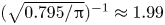$(\sqrt {0.795/{\rm \pi} })^{-1} \approx 1.99$, which is clearly somewhat higher. Saffman & Szeto (Reference Saffman and Szeto1980) also mention earlier studies which had found critical values of $1.7$ or $1.9$ ‘depending on how the vortex radius was defined’. This question of how to quantify vortex size has been investigated in more detail since their work and it is perhaps more interesting to compute the value of $a/b$ where, in this case, $b = 2$ is the distance between the vortex centroids and

(5.1)\begin{equation} a = \sqrt\frac{J }{\varGamma}, \end{equation}

is a measure of the vortex core size proposed by Meunier et al. (Reference Meunier, Ehrenstein, Leweke and Rossi2002) where $J$ is defined in (2.18). A graph of $a/b$ against ${\mathcal {A}}$ is shown in figure 3. At the maximum value of the vortex area ${\mathcal {A}}$ above which equilibria no longer exist we find $a/b \approx 0.260$. The value of $a/b$ does not itself reach a maximum at this point of maximal area, however, and it continues to increase even as the vortex area starts to decrease. The quantity $a/b$ reaches its maximum value of $a/b \approx 0.283$ at the critical configuration where the two vortices almost touch. The values $0.260$ and $0.283$ are not hugely different but both values are larger than the theoretical value of 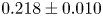$0.218\pm 0.010$ proposed by Meunier et al. (Reference Meunier, Ehrenstein, Leweke and Rossi2002) (see also the discussion in Leweke et al. Reference Leweke, Dizés and Williamson2016). All these discrepancies with other vortex models are likely to be attributable to the concentration of vorticity in the vortex boundaries, i.e. the contribution $q {\mathcal {P}}$ to the total vortex circulation, which is a feature peculiar to the hollow vortex model. Figure 3 also shows the split of the unit circulation $\varGamma =1$ of each vortex between the two contributions $q {\mathcal {P}}$ and $2 \varOmega {\mathcal {A}}$ and reveals that even past the maximum area configuration most of the circulation of the vortices is held in the vorticity concentrated on their boundaries.

Figure 3. Graphs of $a/b$, with $a$ defined in (5.1), $q {\mathcal {P}}$ and $2 \varOmega {\mathcal {A}}$, as functions of ${\mathcal {A}}$.

Figure 4 shows typical vortex shapes for $\rho =0.05, 0.106$ and $\rho =0.3$; the vortices for $\rho =0.106$ correspond to the maximum area configuration. As the critical configuration is approached the two vortices extend thin ‘fingers’ towards the centre of rotation. The calculations suggest that the tips of these fingers draw arbitrarily close together without blow-up of any physical quantities. The near-critical configuration, with $\rho = 0.415$, is shown in figure 5 with an inset showing the near-touching tips of the fingers protruding from each vortex towards the centre of rotation. Numerically the radius of curvature of the tip becomes so small that eventually the numerical method loses accuracy by the growth in contributions from the high-order modes and small oscillations of the vortex boundary in the vicinity of the fingers tips; with $N=64$ modes this is found to occur, however, only after the tips of the two vortices are approximately distance $10^{-4}$ apart (recall that we have normalised the length scale via (4.27)).

Figure 4. Typical equilibrium shapes of the hollow vortices in the corotating frame for $\rho =0.05, 0.106$ and $\rho =0.3$. The vortex centroids are fixed at $\pm \textrm {i}$. The case with $\rho =0.106$ is the maximum area solution. $(a)\,\, \rho = 0.05;\, (b)\,\, \rho = 0.106;\, (c)\,\, \rho = 0.3.$

Figure 5. Near-critical shape of two corotating hollow vortices for $\rho =0.415$. The inset shows a magnified view of the two near-touching ‘fingers’ from each vortex near the centre of rotation.

This evidence suggests that, with higher numerical resolution, the vortices will come arbitrarily close to touching at the origin as $\rho$ increases further. Instead of a higher-resolution numerical investigation, we adopt a different strategy to explore this possibility and ask instead about a single isolated rotating hollow vortex. No solutions for such an object have yet been reported in the literature, so we will adapt our methods and investigate this in the next section. What is known is that the only solution for an isolated non-rotating hollow vortex is a circular one (Llewellyn Smith & Crowdy Reference Llewellyn Smith and Crowdy2012). But what happens if a single hollow vortex is allowed to rotate steadily? Answering this question turns out to give significant insight into the limiting two-vortex configuration depicted in figure 5.

6. A single rotating hollow vortex

An advantage of conformal mapping method is that the case of a single rotating hollow vortex can be formulated immediately with only minor changes as the $\rho \to 0$ limit of the problem already formulated in the annulus. A single rotating hollow vortex is defined as a vortex of total circulation $\varGamma$ rotating steadily with angular velocity $\varOmega$ containing fluid in solid body rotation with this same angular velocity and with fluid of speed $q$ on its boundary. Now the conformal mapping to the fluid region exterior to the single vortex is from the unit disc $|\zeta | < 1$. Specifically, the conformal mapping with $\zeta =0$ mapping to infinity now takes the form

(6.1)\begin{equation} z = Z(\zeta) = \textrm{i} d \left [ \frac{1 }{\zeta} +\sum_{n \ge 1} a_n \zeta^n \right ], \end{equation}

where $\lbrace a_n | n \ge 1 \rbrace$ are a set of real coefficients to be found. To highlight the similarities with the two-vortex problem we will use the same notation already used in that problem with the understanding that the context is now different. It is clear that

(6.2)\begin{equation} \zeta Z'(\zeta) = \textrm{i} d \left [ - \frac{1 }{\zeta}+ \sum_{n \ge 1} n a_n \zeta^n \right ], \end{equation}

so that the requisite integral expression for $a_n$ in terms of $\zeta Z'(\zeta )$ in this case is

(6.3)\begin{equation} a_n = -\frac{1 }{2 {\rm \pi}d n}\oint_{C_0} Z'(\zeta) \frac{\textrm{d} \zeta }{\zeta^{n} },\quad n \ge 1.\end{equation}

Furthermore, $W_\varGamma (\zeta )$ now simplifies to

(6.4a,b)\begin{equation} W_\varGamma(\zeta) = \frac{\textrm{i} \varGamma }{2 {\rm \pi}} \log \zeta,\quad \zeta W_\varGamma'(\zeta) = \frac{\textrm{i} \varGamma }{2{\rm \pi}}.\end{equation}

The time scale of the flow is fixed by setting $\varGamma =2$ since we proceed on the assumption that this single-vortex configuration will connect in some way to the two-vortex configuration, each having circulation $\varGamma =1$, studied previously. The condition on the vortex boundary is again given by (4.4)

(6.5)\begin{equation} {\textrm{i} \zeta H'(\zeta) }= -q|Z'(\zeta)| + \varOmega \overline{Z(\zeta)} {\zeta Z'(\zeta) } - {\textrm{i} \zeta W_\varGamma'(\zeta) },\quad \zeta \in C_0. \end{equation}

The formulation again leads to two Schwarz problems for analytic functions in the unit disc, and since the unit disc is simply connected there are no longer any solvability conditions. We have

(6.6)\begin{equation} \textrm{Re}[\zeta H'(\zeta)] = R_0(\zeta),\quad \zeta \in C_0, \end{equation}

with $R_0(\zeta )$ still given by formula (4.7) and this is a Schwarz problem in the disc for the analytic function $\zeta H'(\zeta )$. Its solution is furnished by the Poisson integral formula

(6.7)\begin{equation} \zeta H'(\zeta) = \frac{1 }{2 {\rm \pi}\textrm{i}} \oint_{C_0} \frac{\textrm{d} \zeta' }{\zeta'} \left (\frac{\zeta'+\zeta }{\zeta'-\zeta} \right ) R_0(\zeta') + \textrm{i} c_1, \end{equation}

where the real constant $c_1=0$ in order to avoid $H(\zeta )$ having a logarithmic singularity at $\zeta =0$. If we now define a modified function

(6.8)\begin{equation} F(\zeta) \equiv \log (\zeta Z'(\zeta)) + \log \zeta \end{equation}

then the logarithmic singularities of both functions at $\zeta =0$ cancel out. Then

(6.9)\begin{equation} \textrm{Re}[F(\zeta)]= \tilde T_0(\zeta),\quad \zeta \in C_0, \end{equation}

where

(6.10)\begin{equation} \tilde T_0(\zeta) \equiv \log(S_0(\zeta)) + \log |\zeta|. \end{equation}

This is the second Schwarz problem for the analytic function $F(\zeta )$ in the unit disc and the Poisson integral formula again provides the required solution.

The same iterative scheme as described in § 4.1 can now be deployed. In all results to follow the Laurent series (6.1) is truncated at $N=32$ terms. Since the vortex centroid is expected to remain at the origin the length scale is now set by fixing the vortex area ${\mathcal {A}}= {\rm \pi}$ with the vortex perimeter ${\mathcal {P}}$ now used as the continuation parameter starting from a circular vortex configuration of unit radius where

(6.11a–d)\begin{equation} {\mathcal{A}} = {\rm \pi},\quad {\mathcal{P}} = 2 {\rm \pi},\quad d=1,\quad a_n = 0,\quad n =1, \ldots, N. \end{equation}

Since this circular configuration is degenerate – a circular vortex is an equilibrium for any values of $q$ and $\varOmega$ satisfying (2.10) – to bifurcate from this trivial branch it is necessary to seed the iteration with a non-zero initial value of $a_1$ which encodes elliptical distortions to the circular vortex, that is, distortions with a $2$-fold rotational symmetry about the origin. Indeed, a local analysis can be used to determine analytically the values of $q$ and $\varOmega$ at which steady solution branches with non-zero $a_1$ bifurcate from the circular solution. It can be posed that

(6.12a,b)\begin{equation} Z(\zeta) = \textrm{i} d \left[ \frac{1 }{\zeta}+ {\epsilon a_1} \zeta + \ldots \right ],\quad H(\zeta) = \epsilon h_2 \zeta^2 + \ldots,\quad \epsilon \ll 1, \end{equation}

where $h_2$ is the leading coefficient of $H(\zeta )$. These are the forms for an elliptical perturbation expected theoretically. These can be substituted into the boundary condition (6.5) which can then be linearised in $\epsilon$. Both sides of this boundary condition can be expanded as a Laurent series convergent for $\zeta \in C_0$ and, on equating powers of $\zeta$ in these Laurent series, the conditions

(6.13a,b)\begin{equation} \frac{\varGamma }{\rm \pi} = d q + \varOmega d^2,\quad \frac{q }{2} = d \varOmega \end{equation}

are deduced on equating the coefficients of $\zeta ^0$ and $\zeta ^{-2}$ respectively. The first of these is just a restatement of condition (2.10). With $\varGamma =2$ and $d=1$ we can solve these two equations for $q$ and $\varOmega$:

(6.14a,b)\begin{equation} q = \frac{2 }{3 {\rm \pi}},\quad \varOmega = \frac{1 }{3 {\rm \pi}}. \end{equation}

More generally, although we do not explore them here because they are tangential to our present goals, it is expected that there exist bifurcations, from a circular vortex, of steadily rotating hollow vortices with $m$-fold rotational symmetry about the origin of which the case of particular interest here is $m=2$.

Figure 6 shows a graph of $q$ and $\varOmega$ against the rescaled perimeter ${\mathcal {P}}/2 {\rm \pi}$ for the family of single rotating hollow vortex solutions found using the numerical scheme. The two crosses shown on the graphs confirm that the numerical method retrieves the theoretical values (6.14a,b) just predicted and this provides a check on the numerical method.

Figure 6. Graphs of $q$ and $\varOmega$ against ${\mathcal {P}}/2 {\rm \pi}$ for a single rotating hollow vortex. Values for the critical configuration are indicated by small circles. The $q$-curve intersects the axis at the cross at $1/(3 {\rm \pi})$, the $\varOmega$-curve at the red cross at $2/(3{\rm \pi} )$ as predicted in (6.14a,b).

The shapes of the hollow vortex for ${\mathcal {P}}/2 {\rm \pi}= 1.05, 1.5$ and $2.5$ are shown in figure 7. As the perimeter increases the vortex is found to become elongated along the direction of the $y$-axis and eventually develop a ‘waist’ where the two sides of the vortex draw closer together. Eventually a limiting configuration at 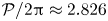${\mathcal {P}}/2 {\rm \pi}\approx 2.826$ is found where two distinct parts of the vortex boundary appear to almost touch; the calculations are terminated just before this occurs since such a touching configuration is not physically admissible. Figure 8 shows the (rescaled) near-critical configuration: two distinct parts of the vortex boundary are drawing close together and, as shown in the inset close-up, are separated by a distance of the order of $10^{-4}$.

Figure 7. Typical equilibrium shapes of a single hollow vortex in the corotating frame for 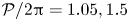${\mathcal {P}}/2{\rm \pi} = 1.05, 1.5$ and $2.5$. The vortices all have area ${\mathcal {A}}={\rm \pi}$. $(a)\,\, \mathcal {P}/2{\rm \pi} = 1.05;\, (b)\,\, \mathcal {P}/2{\rm \pi} = 1.5;\, (c)\,\, \mathcal {P}/2{\rm \pi} = 2.5.$

Figure 8. Near-critical shape of single rotating hollow vortex for ${\mathcal {P}}/2 {\rm \pi}= 2.826$ rescaled so that it has the same area as the two near-critical rotating hollow vortices of figure 5.

All the calculations point to the formation of what we refer to as a topological singularity: it is clear visually that the shape of the limiting configuration of the single rotating hollow vortex as its waist thins and the two sides of the vortex draw close together is very similar to the limiting configuration of the two rotating hollow vortices as the two ‘fingers’ protruding from each vortex nearly touch. Indeed, the calculations point to the two scenarios producing the same limiting shape, albeit via topologically distinct limits: compare figures 5 and 8 where the latter figure has been rescaled so that the vortex has the same area as the sum of the two vortices in figure 5. Quantitatively, if we introduce the length scale factor $L$ based on the critical area ${\mathcal {A}}_{crit} = 0.311$ of each of the two corotating vortices shown in figure 2, namely,

(6.15)\begin{equation} L = \left (\frac{2 \times 0.311 }{\rm \pi} \right )^{1/2} \end{equation}

and use this to rescale the critical values of $q=0.1050$ and $\varOmega =0.0212$ for the single vortex indicated in figure 6 we find

(6.16a,b)\begin{equation} q^* = \frac{q }{L} = \frac{0.1050 }{L} = 0.236,\quad 4 {\rm \pi}\varOmega^* = 4 {\rm \pi}\left ( \frac{\varOmega }{L^2} \right ) = 4 {\rm \pi}\left ( \frac{0.0212 }{L^2} \right ) = 1.346, \end{equation}

which are very close to the values indexed by daggers in table 1 and corresponding to the near-critical configuration of two hollow vortices shown in figure 5. We offer this as evidence that the single-vortex and two-vortex scenarios are tending to the same limiting configuration. The limiting ‘touching’ configuration itself is not physically admissible since, by the symmetry of the arrangement, the origin at which the vortices touch would need to be a stagnation point meaning that, for a continuous limit, we would need $q \to 0$. Figure 9 superposes a close-up of this topological transition based on the numerical calculations closest to transition calculated using both the single-vortex and two-vortex numerical codes.

Figure 9. Illustration of the topological singularity: the topology of the vortex boundary changes but all physical quantities ($q$ and $\varOmega$) are continuous across the singularity.