


1. Introduction
Wave breaking is commonly considered to be the process that limits the height (steepness) that surface gravity waves may reach. However, its precise definition may often vary; for clarity we define wave breaking as the point at which the surface becomes unstable to small perturbations and wave motion is no longer reversible. For purely travelling waves, breaking has known implications on maximum wave height. Stokes (Reference Stokes1880) first proposed that a crest enclosing an angle of  $120^\circ$ was the limiting form prior to breaking for a progressive surface gravity wave on deep water (see Zhong & Liao (Reference Zhong and Liao2018) for a study of all water depths). This limit provides an upper bound of wave height
  $h$ for a given wavenumber
  $k$ and corresponds to a steepness of
  $kh/2=0.44$. Stokes's proposed waveform corresponds to a two-dimensional or infinitely long-crested wave. In reality, ocean waves are three-dimensional, and their typical crest length depends on the directional spreading of the local sea state. Directional spreading has a strong effect on the onset of wave breaking and the limiting steepness of waves (e.g. She, Greated & Esson Reference She, Greated and Esson1994; Johannessen & Swan Reference Johannessen and Swan2001; Babanin et al. Reference Babanin, Waseda, Kinoshita and Toffoli2011; Latheef & Swan Reference Latheef and Swan2013). An axisymmetric standing wave is, in essence at the point of focus, an infinitely short-crested wave. Hence, the breaking behaviour of real-world ocean waves lies between these two canonical forms, unidirectional (two-dimensional) or infinitely long-crested, and axisymmetric (three-dimensional) or infinitely short-crested. Axisymmetric surface waves occur in a number of scenarios and are often associated with jet formation. In cylindrical vessels, Faraday resonance can create axisymmetric waves (Miles Reference Miles1984), and axisymmetric jetting behaviour is common when features with rotational symmetry, such as bubbles and droplets, encounter a free surface or wall (e.g. Blake & Gibson Reference Blake and Gibson1981; Longuet-Higgins & Oguz Reference Longuet-Higgins and Oguz1997; Zeff et al. Reference Zeff, Kleber, Fineberg and Lathrop2000). See table 1 in Basak, Farsoiya & Dasgupta (Reference Basak, Farsoiya and Dasgupta2021) for a comprehensive overview of theoretical, numerical and experimental studies involving such behaviour. These examples occur across a range of scales with varying relative importance of the effects of viscosity, capillarity and gravity. However, as suggested by Longuet-Higgins (Reference Longuet-Higgins1983), some features such as jet formation may be ubiquitous.
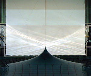
The FloWave Ocean Energy Research Facility at the University of Edinburgh is a circular wave tank surrounded by wavemakers. The geometry and wave making capacity of this tank makes it particularly adept at generating axisymmetric waves. As a demonstration of this ability, a wave which is colloquially known as the ‘spike wave’ was developed. The spike wave is created when the wavemakers that surround the tank are driven in unison to create many axisymmetric waves of different frequencies that focus at the centre of the tank. Figure 1 shows an image of the spike wave, which at its peak forms a singular-looking jet of water over 6 m in height. The striking nature of this wave has attracted the attention of several popular science outlets (e.g. https://www.youtube.com/watch?v=iWKFPTgkpXo, https://www.ed.ac.uk/news/staff/2016/wave-image-wins-photography-prize), but the fluid mechanics that leads to its formation are yet to be explored. We will show the spike wave created in the FloWave tank is a unique example of a breaking axisymmetric standing wave, at an absolute scale much larger than previously observed. Herein, we examine this wave using several measurement techniques and counterpart numerical simulations to better understand the fluid mechanics of the spike wave and, consequently, axisymmetric standing wave breaking. For completeness, we note that the term ‘standing wave’ has multiple connotations; we use this term to refer to the surface motion created when waves of the same frequency propagate in opposing directions. This definition does not imply time periodicity, resonance, or an enclosed flow.

Figure 1. Image of the ‘spike wave’ created in the FloWave circular wave tank.
Guthrie (Reference Guthrie1875), Rayleigh (Reference Rayleigh1876), Honda & Matsushita (Reference Honda and Matsushita1913) and Fultz & Murty (Reference Fultz and Murty1963) examined periodic axisymmetric standing waves generated by Faraday resonance in closed cylinders. The predominant focus of these studies was on the nonlinear resonant behaviour of such waves, particularly their generation and frequency of oscillation. Because of this focus, the waves these authors examined were of small amplitude and far from breaking. In similar experiments, Longuet-Higgins (Reference Longuet-Higgins1983) created standing waves, increasing their amplitude to the point that they were ‘overdriven’ or breaking, to illustrate the subsequent formation of hyperbolic jets. Longuet-Higgins (Reference Longuet-Higgins1983) suggested that hyperbolic jet formation is a predominantly inertial phenomenon, ubiquitous in free surface flows. Considerable effort has been directed at determining scaling laws for jet formation in collapsing cavities, predominantly focusing on those created by small bubbles and droplets (e.g. Zeff et al. Reference Zeff, Kleber, Fineberg and Lathrop2000; Ghabache, Séon & Antkowiak Reference Ghabache, Séon and Antkowiak2014; Van Rijn et al. Reference Van Rijn, Westerweel, Van Brummen, Antkowiak and Bonn2021). Notably, Ghabache et al. (Reference Ghabache, Séon and Antkowiak2014) use energy arguments to demonstrate that jet height scales with  $H(H/L)^2$, where
  $H$ and
  $L$ are cavity depth and width, respectively. Ghabache et al. (Reference Ghabache, Séon and Antkowiak2014) assume that jet behaviour is inertia dominated and use mass and momentum conservation to derive a self-similar velocity profile for the jet. The velocity profile is used to determine kinetic energy, and an expression for jet height is derived by balancing this with the initial potential energy of the cavity.
Using a perturbation expansion approach, Mack (Reference Mack1962) derived analytical expressions describing periodic axisymmetric standing waves up to third order in amplitude. Tsai & Yue (Reference Tsai and Yue1987) used expressions based on Fourier–Dini series to numerically model periodic axisymmetric standing waves, which offered improved accuracy for shallow water depths when compared with Mack's solutions. However, Tsai & Yue (Reference Tsai and Yue1987) observed that at amplitudes approaching wave breaking the convergence of their method is poor. Axisymmetric jet formation and break-up has been modelled successfully using multi-phase computational fluid dynamics (CFD) simulations of bursting bubbles (e.g. Duchemin et al. Reference Duchemin, Popinet, Josserand and Zaleski2002) and gravity–capillary waves (e.g. Basak et al. Reference Basak, Farsoiya and Dasgupta2021).
Owing to their reduced complexity, more progress has been made modelling two-dimensional (2-D) standing waves numerically and analytically to the point at which breaking occurs. The limiting form of periodic 2-D standing waves prior to breaking was examined by Penny & Price (Reference Penny and Price1952). Using three arguments, based on stability, surface continuity, and a fluid's inability to withstand tension, they showed that downward fluid acceleration cannot exceed gravity  $g$. Assuming that the free surface is expressible as a Taylor series, Penny & Price showed that this limit is reached when a crest encloses an angle of
  $90^\circ$ (using the same approach Mack (Reference Mack1962) derived a ‘limiting’ angle of
  $2\tan ^{-1}(\sqrt {2})=109.47^\circ$ for a periodic axisymmetric standing wave). This limiting form has an amplitude approximately
  $50\,\%$ greater than the steepest travelling wave. Using a fractal approach to examine breaking, Longuet-Higgins (Reference Longuet-Higgins1994) showed that the acceleration of the free surface
  $\ddot {\eta }$ for a standing wave crest lies within the bounds
  $-g<\ddot {\eta }<\infty$. A 2-D standing wave enclosing an angle of
  $90^\circ$ was reproduced experimentally by Taylor (Reference Taylor1953). Numerical simulations of periodic 2-D standing waves carried out by Mercer & Roberts (Reference Mercer and Roberts1992) demonstrated that waves enclosing an angle smaller than
  $90^\circ$ can be created. Their results also showed that, as
  $\ddot {\eta }$ approaches
  $-g$, wave height does not increase monotonically, and bifurcation occurs. Schultz et al. (Reference Schultz, Vanden-Broeck, Jaing and Perlin1998) produced similar numerical results to Mercer & Roberts (Reference Mercer and Roberts1992) while also including the effects of surface tension, suggesting that surface tension was necessary to reproduce the experimental observations in Taylor (Reference Taylor1953). Using a highly resolved numerical model, Wilkening (Reference Wilkening2011) examined the behaviour of quasi-periodic standing wave solutions to the water wave equations as acceleration approaches the limit of
  $-g$. Wilkening's simulations show small-scale resonant oscillations form at the wave crest, which cause multiple bifurcations; he suggests that the self-similarity observed in previous studies is in fact a result of insufficient resolution. The small-scale oscillations reported by Wilkening (Reference Wilkening2011) could also be related to phenomena discussed in Tsai & Yue (Reference Tsai and Yue1987) and Roberts & Schwartz (Reference Roberts and Schwartz1983), in which oscillations are observed at the highest modes retained in their numerical solutions, which are attributed to non-uniqueness of their solutions and described as ‘non-physical’ therein. We also note that for travelling wave groups the steepness at which breaking occurs reduces as bandwidth increases (Wu & Yao Reference Wu and Yao2004), further limiting the potential applicability of a single limiting form to quasi-periodic waves. Summarising, the above experimental and numerical studies demonstrate that a limiting form of 2-D standing waves may not exist and raise the question whether the same is true for axisymmetric standing waves.
Although a single limiting form may not exist for standing waves, a characteristic that is consistently reported in the literature is that, when standing waves break or are ‘overdriven’, jet formation occurs. Longuet-Higgins (Reference Longuet-Higgins2001b) and Longuet-Higgins & Dommermuth (Reference Longuet-Higgins and Dommermuth2001a,Reference Longuet-Higgins and Dommermuthb) examine jet formation on 2-D standing waves numerically using a Lagrangian system of equations (Balk Reference Balk1996) and a boundary integral method (Longuet-Higgins & Cokelet Reference Longuet-Higgins and Cokelet1976). They do so by prescribing arbitrary initial surface velocity or elevation and time marching these initial conditions. Prescribing initial conditions in such a way does not guarantee periodic surface motion, and hence the waves they examine are not purely periodic. They show that predicted fluid acceleration is not sensitive to the scale of waves (i.e. amplitude or height), but is determined by the shape of the trough prior to jet formation (i.e. steepness or radius of curvature), and report crest velocities exceeding  $1.7$ times the linear phase speed. Water depth has also been shown to affect jet formation, with larger crests predicted in finite depth than in deep-water simulations of standing waves (Wilkening & Yu Reference Wilkening and Yu2012). Longuet-Higgins (Reference Longuet-Higgins1983) demonstrated, when analysing bubbles approaching a free surface (Blake & Gibson Reference Blake and Gibson1981), that once a jet has formed subsequent evolution takes the form of a jet with a hyperbolic shape. The jet model presented in Longuet-Higgins (Reference Longuet-Higgins1983) suggests that jet formation and hence indirectly breaking occurs at angles of
  $90^\circ$ and
  $109.47^\circ$ for 2-D and axisymmetric standing waves, respectively. At these angles, the model predicts a large positive ‘jolt’ in acceleration, not
  $-g$. Longuet-Higgins (Reference Longuet-Higgins2001a) presented an asymptotic jet model for 2-D standing waves that does not exhibit a singularity at
  $90^\circ$. Hence, this apparent jolt reported in Longuet-Higgins (Reference Longuet-Higgins1983) may be an artefact of the chosen model. Determining the point at which wave breaking occurs for axisymmetric standing waves in general and in the experiments presented herein in particular is a challenge in its own right. For travelling waves, visual identification of wave breaking is straightforward (Babanin Reference Babanin2011). For standing waves, wave motion and jet formation may both result in vertical movement of the free surface, and a clear distinction between the two phenomena does not exist. Once a wave crest has transformed into a free-falling jet, breaking and irreversible surface motion has clearly occurred. However, the onset of breaking may have occurred prior to this. Thus free-falling jet formation alone may not be a useful indicator of wave breaking onset.
In the following paper, we investigate the mechanisms that create the spike wave shown in figure 1 with the aim of revealing its fluid mechanics and improving understanding of breaking free surface gravity waves. We provide details of our experiments in § 2. We then address the following questions. First, is the (nonlinear) wave crest amplitude limited by breaking and how is it related to the linear input amplitude based on linear dispersive focusing (§ 3)? Second, what are the mechanisms that lead to the generation of the spike wave, and does ‘nonlinear focusing’ (see e.g. Dudley et al. (Reference Dudley, Genty, Mussot, Chabchoub and Dias2019) for a review) play a role (§ 4)? Third, do the jets that form evolve in a similar manner to observations at smaller absolute scales and can this be modelled (§ 5)? Fourth, how may we identify wave breaking, and do the observed mechanisms of breaking and air entertainment relate to previous studies (§ 6)? Finally, we draw conclusions in § 7.
2. Experimental method
Experiments were conducted in the FloWave Ocean Energy Research Facility (www.flowave.eng.ed.ac.uk) at the University of Edinburgh. The facility consists of a  $25$ m diameter circular wave basin, surrounded by 168 active-absorbing force-feedback wavemakers, with a water depth of
  $2$ m. This circular geometry enables the creation of waves in all directions and thus readily facilitates the generation of axisymmetric waves. Owing to the large amplitude of the waves examined in our experiments (0.1–6.0 m), it was not possible to make measurements using wave gauges in all cases. To measure waves larger than approximately
  $0.5$ m in amplitude, we employed two alternative free surface measurement techniques: calibrated image processing and floating surface markers. Figure 2 shows our experimental set-up. Further details of the measurement techniques we use are provided in Appendix A with details of the wave gauge configuration in Appendix A.1, the procedure to obtain calibrated high-speed images of the free surface in Appendix A.2 and the free surface measurements using floating markers and the Qualisys system in Appendix A.3.

Figure 2. Experimental set-up with (a) diagram of the wave tank, showing wave gauge array A, Qualisys infra-red (IR) cameras, high-speed camera, calibration plane and screen; and (b) photograph of the wave tank and the screen.
2.1. Experimental matrix
To gain an understanding of the mechanisms that underlie the ‘spike wave’, we recreate the wave at different amplitudes. Increasing the amplitude gradually allows for observation of linear and nonlinear focusing mechanisms and the onset of breaking and jet formation. The largest amplitude we created was limited by the vertical clearance above the wave tank ( ${\approx }7\ \textrm {m}$) and the field of view of the camera set-up. Table 1 lists the increments over which we increase the linear input amplitude
  $A_{0}$ of our experiments, from
  $0.2$ to
  $1.53$ m, where
  $A_{0}$ corresponds to the maximum amplitude of the surface elevation at the centre of the tank according to linear theory. Details are also provided of the types of measurement available for each experiment.
Table 1. Matrix of experimental input parameters:  $r_0=6.13$ m is the predicted radius of the linear fundamental mode with corresponding wavenumber
  $k_0={\rm \pi} /r_0=0.51\ \textrm {m}^{-1}$. Total linear wave height
  $H_0$ is equal to
  $1.408A_0$.

The ‘spike wave’ was designed to produce a single, highly repeatable large crest in space and time. Producing a temporally localised wave group minimises the build-up of reflected waves, which act as background motion in the tank and have a significant effect on focusing and jet formation. Moreover, it is not possible to produce a single-frequency resonant mode in the tank, as is done in vibrating cylindrical containers with fixed side walls, as this would require large surface motion at the circumference of the tank where the wavemakers are located. To create a large temporally and spatially localised wave, a broad-banded spectrum was used to produce a focused wave group. The shape of the spectrum was chosen considering the capability of the wavemakers and is based on an International Towing Tank Conference (ITTC) spectrum (Mathews Reference Mathews1972), which follows the general form
 \begin{equation} S(\,f)= \frac{\alpha}{f^5}\exp\left(\frac{\beta}{f^4}\right), \end{equation}
where  $\alpha$ is scaling parameter which is adjusted to achieve the desired amplitude
  $A_0$ at focus, f is frequency and
  $\beta =-0.44/\bar {T}^4$ is a shape parameter. All our experiments were carried out with mean period
  $\bar {T}=2.3$ s, which gives a peak period
  $T_p=2.8$ s.
The repeat time of each experiment was 64 s, which means discrete wave components are generated with a frequency resolution of  $\delta f= 1/64 = 0.0156$ Hz. The discrete wave components at each frequency are generated so that they are all in phase at the centre of the tank (based on linear theory). Figure 3 shows time series of surface elevation at the centre of the tank based on the wavemaker inputs, linear wave theory and the underlying amplitude spectrum for all experiments.

Figure 3. Experimental input conditions: (a) linearly predicted free surface elevation  $\eta ^{(1)}$ at the point of focus (
 $r=0$), and (b) corresponding discrete amplitude spectra
  $\hat {\eta }^{(1)}$ for all experiments.
Between experiments, the only parameter varied was the input linear amplitude at focus  $A_0$. Based on these inputs, the waves have a characteristic wavelength
  $\lambda _0=12.2$ m (wavenumber
  $k_0=0.51\ \textrm {m}^{-1}$,
  $\lambda _0=2{\rm \pi} /k_0$), which was calculated as twice the radial position of the wave trough at the time of linear focus,
  $t=0$ (i.e.
  $r_0=6.13$ m). Accordingly, the characteristic water depth of the waves we create is
  $d/r_0=0.326$ or
  $k_0d=1.02$, which is considered non-critical (Mack (Reference Mack1962) predicts critical depth to occur at
  $d/r_0 \approx 0.2$; at critical depths nonlinearly generated higher modes of the fundamental frequency are of the same order of magnitude as first-mode oscillations) or intermediate to deep. At the scale of our experiments, the Bond number
  ${Bo}=(\rho g)/\sigma k_0^2$ is of the order
  $10^{5}$, where
  $\rho$ is density and where we assume the surface tension of water
  $\sigma =72\ \textrm {mN}\ \textrm {m}^{-1}$. For small-scale surface oscillations, as predicted by Wilkening (Reference Wilkening2011), this increases to
  $10^{2}$. It is possible that these small-scale surface oscillations will experience an altered effective gravity owing to the local fluid acceleration, and thus the Bond number calculated using constant
  $g$ may be misleading. We nevertheless conclude surface tension effects will unlikely be important.
A minimum settling time of  $10$ min was completed between experiments to allow for the dissipation of background motion. Failing to allow for sufficient time between experiments has a strong effect on crest shape and jet formation, resulting in a less sharp waveform and a reduced crest amplitude.
3. Experimental observations
In this section, we present our experimental observations, and draw comparison with analytical expressions for surface elevation of periodic axisymmetric standing waves and wave breaking limits by Mack (Reference Mack1962) (see Appendix B) thus focusing on maximum crest amplitude. Figure 4 shows images of the waves produced during our experiments as input amplitude was increased (Exp.  $40$ to Exp.
  $75$, left to right), at
  $0.24$ s intervals (top to bottom).

Figure 4. Images of Exp.  $40$ to Exp.
  $75$ (left to right) from
  $t=-0.44$ to
  $0.28$ s in intervals of
  $0.24$ s (top to bottom), where
  $t=0$ corresponds to the time of linear focus. See supplementary material for movies available at https://doi.org/10.1017/jfm.2021.1023 of the experiments shown in this figure.
3.1. Surface elevation
Owing to the amplitude of the waves we create exceeding the size of our wave gauges, we have implemented two image-based (or indirect) methods to measure surface elevation near the wave crest ( $r=0$). In figure 5 we compare measurements of surface elevation plotted as a function of radial position
  $r$ for Exp. 30 and Exp. 75. Surface elevation measured using wave gauges
  $\eta _{G}$ (blue markers), calibrated high-speed images
  $\eta _{I}$ (grey lines) and floating markers
  $\eta _{Q}$ (red dots) are compared at approximately
  $0.16$ s intervals. Exp. 75 is the largest wave we created, and Exp. 30 is the largest experiment for which gauge measurements were made at the centre of the tank (as well as further out). In Exp. 30 surface elevation exceeded the height of the gauge at
  $r=0$, meaning that the measurements produced by this gauge are incorrect at the time of the wave crest. The adjacent gauges were not over-topped and may still be used to validate the indirect measurement techniques near
  $r=0$. In figure 5(a) the indirect measurements of surface elevation,
  $\eta _{I}$ (calibrated images) and
  $\eta _{Q}$ (floating markers), agree well with the gauge measurements shown. As the wave crest reaches a maximum, the surface elevation measured using the floating markers differs slightly from the image-based measurements. At instances where the free surface experiences significant acceleration, the floating makers will exhibit some degree of inertial behaviour and may not follow the surface exactly. For the crest in figure 5(a),
  $\eta _{Q}$ (floating markers) matches
  $\eta _{G}$ (gauges) closely, so it does not appear that the floating markers are exhibiting observable inertial effects. In Exp. 30 the wave crest is low in the camera's field of view and does not reach the bottom of the screen used to aid edge detection. Therefore, there may be some parallax error in the extracted profile in this case. In Exp. 75, in which surface elevation reaches around
  $6$ m and lies directly in front of the screen, all three techniques compare well and can be combined effectively to capture the extreme surface profile created.

Figure 5. Surface elevation measurements for Exp. 30 (a) and Exp. 75 (b): blue open circles show gauge measurements  $\eta _{G}$, grey lines show measurements from calibrated images
  $\eta _{I}$ and red dots show measurements made with floating markers
  $\eta _{Q}$. Surface elevation is presented at approximately 0.16 s intervals, where artificial ‘velocities’ of 1.5 and
  $12\ \textrm {ms}^{-1}$ have been applied to separate the measurements at different times on the same vertical axis and aid clarity in panels (a) and (b), respectively.
Figure 6 shows surface elevation measured in Exp. 50-75. The top row (a–e), shows surface elevation measured immediately prior to visual observation of the rapid (over 1–2 frames or 8–16 ms) formation of a sharp-cusped wave crest. The bottom row (f–j) shows surface elevation measured at the time when the wave crest reaches a maximum. The rapid formation of a sharp-cusped wave crest is an indication of jet formation and may be an indication of the onset of wave breaking; this hypothesis is examined in more detail in §§ 4.1 and 4.2. As we increase the amplitude of the waves created, the point where a cusp forms occurs earlier and at lower measured amplitude. This potentially contradicts the concept of a limiting waveform, as the onset of breaking does not occur at a fixed amplitude and steepness (the wavelength remains unchanged). The time at which maximum surface elevation is reached is delayed as input amplitude increases, and the maximum surface elevation does not appear to be limited by breaking.

Figure 6. Surface elevation for Exp. 50 to Exp. 75 at the time of observed jet formation (a–e) and maximum elevation (f–j): blue open circles show gauge measurements  $\eta _{G}$, grey lines show measurements from calibrated images
  $\eta _{I}$ and red dots show measurements made with floating markers
  $\eta _{Q}$. In (i,j)
  $\eta _{I}$ is shown by a single marker to aid clarity.
3.2. Maximum amplitude
Owing to imperfect wave generation, the waves may not be produced to the specified input linear amplitude in the wave tank (see table 1). To estimate the actual linear amplitude  $A_0$ of the waves created, we use the measurements from wave gauge array A for Exp. 30 to Exp. 75, and gauge array B for Exp. 10 and Exp. 20. In figure 7(a) the maximum surface elevation
  $A$ measured using the calibrated images (red dots) is plotted as a function of the estimated linear amplitude
  $A_0$. As also shown in figure 6(f–j), as the linear amplitude
  $A_0$ is increased, the maximum surface elevation
  $A$ increases rapidly, reaching a value of
  $6.03$ m for a corresponding linear amplitude of
  $1.03$ m. The purple markers in figure 7(a) also show third-order accurate amplitudes predicted by Mack (Reference Mack1962) for periodic axisymmetric standing waves (calculated using (B2) in Appendix B). Table 2 provides details of the linear and total amplitudes measured during our experiments and simulations.

Figure 7. Maximum surface elevation: (a) shows total amplitude as a function of measured linear amplitude  $A_0$, the grey dashed and dot-dashed line denote Reference StokesStokes’ and Mack's predicted limiting amplitudes, respectively; (b) shows second- and third-order components of amplitude as a function of measured linear amplitude
  $A_0$; (c) shows measured amplitude on logarithmic axes as a function of trough depth prior to jet formation
  $H$, with the black dashed line corresponding to
  $A\propto H^3$. Red filled markers denote measured total amplitude, blue and purple markers denote predicted second-order and third-order amplitudes.
Table 2. Crest amplitudes and jet velocities from experimental observations:  ${\dagger}$ denotes gauge measurements at
  $r=0$ using array B and
  ${\dagger} {\dagger}$ those made using array A (see appendix A); other measurements are made using calibrated images. In the rightmost column, superscripts
  $\star$ and
  $s$ denote peak crest velocities measured in simulations and using images from experiments, respectively. Those without superscripts are calculated as
  $\dot {\eta }_{\tiny {C}}=\sqrt {2g(A-A_{cusp})}$ (see § 4).

Figure 7(b) shows the individual second- and third-order components of wave amplitude. The continuous lines show values predicted by Mack (Reference Mack1962) for periodic axisymmetric standing waves (calculated using (B2)), and the blue dots show values calculated using multi-chromatic second-order theory (Dalzell Reference Dalzell1999) based on linearised measurements. The waves we create are broad banded and hence may not be modelled well as a monochromatic wave (as in Mack (Reference Mack1962)). However, the second-order components predicted by both monochromatic Mack (Reference Mack1962) and multi-chromatic (Dalzell Reference Dalzell1999) theories agree well, which demonstrates the effects of bandwidth are at least negligible at second order; at third order the effects of bandwidth may be more pronounced.
Visual (a sharp-cusped wave crest) and aural (see supplementary movie) signs which may be indicative of jet formation and subsequent wave breaking were observed in Exp. 40 and Exp. 50, respectively. Hence, we believe the onset of breaking may occur between Exp. 30 and Exp. 40, as indicated by the grey shaded area in figure 7(a) (this is confirmed in § 4.1). At amplitudes below this breaking onset, measured amplitude  $A$ follows the monochromatic third-order prediction by Mack (Reference Mack1962) well. Above this breaking onset, measured amplitude begins to increase rapidly.
In figure 7(c), filled markers show total measured jet amplitude  $A_{M}$ plotted as a function of the trough depth prior to jet formation
  $H$. This approximately follows an
  $H^3$ scaling, as predicted in Ghabache et al. (Reference Ghabache, Séon and Antkowiak2014). We emphasise that Ghabache et al. (Reference Ghabache, Séon and Antkowiak2014) predict
  $A$ will scale with
  $H(H/L)^2$; to examine how well this agrees with our data we have assumed a constant cavity diameter
  $L$ in figure 7(c).
4. Generation mechanism
Waves of extreme form and incipient breaking are often associated with nonlinearity and (resonant) instabilities. For periodic axisymmetric standing waves, Mack's third-order solutions predict changes to the dispersion relationship, which cause amplitude-dependent modification to the frequency of oscillation. In the following section, we aim to investigate the mechanisms of focusing (§ 4.1) and of breaking onset (§ 4.2) of the steep axisymmetric waves we create.
4.1. (Non) linear dispersive focusing
Steep surface gravity waves can occur as a result of linear dispersive focusing or, under certain conditions, resonant interactions (‘nonlinear focusing’). To assist in understanding the relative importance of these different focusing mechanisms in the formation of the spike wave, we carry out numerical simulations based on our experiments using the potential-flow solver OceanWave3D (see Appendix C for discussion of the method and convergence).
The red dot-dashed and blue solid lines in figure 8 show simulated surface elevation  $\eta _{\tiny {O}}$ at the point of focus
  $r=0$ (
 $x=0$,
  $y=0$) for grid resolutions
  $\varDelta =0.098$ and
  $\varDelta =0.049$ m, respectively. Simulations were carried out with the same duration for all the experiments (Exp. 10 to Exp. 75). For Exp. 40 onwards the simulations became unstable and stopped prior to completion (cf. figure 8a–i). For Exp. 40 and Exp. 50, numerical instability occurs after the wave crest has formed. As the amplitude of the waves is increased, numerical instability occurs at earlier times. We note that increasing resolution may improve the stability of our simulations at large amplitudes (i.e. Exp. 50 onwards). It may be possible to model aspects of jet formation more accurately using multi-phase CFD (e.g. Duchemin et al. Reference Duchemin, Popinet, Josserand and Zaleski2002). However, the intended use of our simulations is primarily to elucidate the focusing mechanisms of the ‘spike wave’. Our simulations converge (see Appendix C.3) and provide reliable results up until the point of wave breaking (Exp. 40). Increasing resolution further is beyond the scope of the current paper owing to constraints on memory. We note that localised jets on 2-D standing waves have been successfully modelled using potential flow (Longuet-Higgins & Dommermuth Reference Longuet-Higgins and Dommermuth2001a).

Figure 8. Numerically simulated surface elevation  $\eta$ at the point of focus (
 $r=0$) for Exp. 10 to Exp. 75: grey solid lines show linear simulations
  $\eta ^{(1)}_{\tiny {O}}$, grey dotted lines linear simulations with multi-chromatic second-order bound waves super-imposed
  $\eta ^{(1)}_{\tiny {O}} +\eta ^{(2)}_{\tiny {T}}$, red dot-dashed and blue lines show fully nonlinear potential-flow simulations
  $\eta _{\tiny {O}}$ at grid resolutions
  $\varDelta =0.098$ and
  $0.049$ m, respectively. Nonlinear potential flow simulations are shown until the time they become unstable. In (a,b), black dots show surface elevation
  $\eta _G$ measured using a wave gauge during Exp. 10 to Exp. 30, which agree well with the nonlinear potential-flow simulations (the lines overlap).
In figure 8(a,b) black dots shows gauge measurements from our experiments, which compare well with numerical simulations. At larger amplitudes, we compare numerical results with measurements from calibrated images in figures 9 and 10, which show Exp. 40 and Exp. 50, respectively. In these figures, numerical surface elevation  $\eta _{\tiny {O}}$ (m) has been transformed to pixels and super-imposed onto the images using our in-plane calibration. For Exp. 40 in figure 9 our simulations compare well with our experiments, replicating the sharp crest that forms. However, for Exp.
  $50$ in figure 10 the sharp crest that forms is not captured, and the simulations become unstable at around
  $t=0.04$ s. Our simulations become unreliable the near the wave crest for Exp.
  $50$ onwards. However, away from the crest our simulations agree with well the images. Therefore, we focus the analysis of our simulations on times prior to crest formation for Exp.
  $50$ onwards, for which simulations are stable and accurate.

Figure 9. Numerically simulated surface elevation super-imposed on calibrated images from Exp. 40: each panel shows calibrated images at different instances in time, gold lines show surface elevation from nonlinear potential-flow simulations  $\eta _{O}$.

Figure 10. Numerically simulated surface elevation super-imposed on calibrated images from Exp. 50: each panel shows calibrated images at different instances in time, gold lines show surface elevation from nonlinear potential-flow simulations  $\eta _{O}$. The simulations become unstable at around
  $t=0.04$ s, after which they are not shown.
The grey solid lines in figure 8 show surface elevation from simulations carried out retaining only linear terms in the governing equations  $\eta _{\tiny {O}}^{(1)}$. The grey dotted lines show the results of the linear simulations with second-order bound components super-imposed,
  $\eta ^{(1)}_{\tiny {O}} +\eta ^{(2)}_{\tiny {T}}$, where the second-order bound component
  $\eta ^{(2)}_{\tiny {T}}$ are calculated using multi-chromatic second-order theory (Dalzell Reference Dalzell1999). The predicted second-order accurate crest acceleration is less than
  $-g$ for Exp. 60 onwards, suggesting the solutions have become invalid for these amplitudes. By comparing linear and fully nonlinear surface elevation in figure 8, we can examine the relative importance of linear and nonlinear focusing mechanisms. As amplitude is increased from Exp. 10 to Exp. 50, the linearly and nonlinearly simulated wave crest occur at approximately the same time (within
  $\pm 0.05$ s, or
  $\pm 0.018T_p$); a clear phase shift does not occur.
In figure 11 we compare numerically simulated linear and nonlinear surface elevation plotted as a function of radial position  $r$ for Exp. 10 to Exp. 40. We observe that the majority of the surface motion is effectively linear, with only the region around the crest (
 $r\pm 0.05\lambda _0$) showing significant nonlinearity at the time of maximum crest elevation (solid lines). At times prior to the maximum crest, the entire surface is effectively linear (dotted and dashed lines show surface elevation at the time of minimum trough). It appears that the localisation in space and time of the waves we create limits the duration and spatial extent of nonlinear contributions that may lead to resonant changes to focusing (see Appendix D for a full decomposition of the simulations for Exp. 40 into their different (non)linear components). The majority of surface motion leading up to the spike wave is linear. Nonlinearity clearly affects the total crest height we observe, but perhaps not in the quasi-resonant manner typical associated with steep travelling waves (e.g. Janssen Reference Janssen2003).

Figure 11. Numerically simulated surface elevation  $\eta$ as a function of radial position
  $r$ at the time of maximum crest
  $\eta _{\tiny {C}}$ (solid lines) and minimum trough
  $\eta _{\tiny {T}}$ (dotted and dashed lines) for Exp. 10 to Exp. 40 (left to right): grey and red lines show linear
  $\eta ^{(1)}_{\tiny {O}}$ and nonlinear
  $\eta _{\tiny {O}}$ simulations, respectively.
4.2. Curvature collapse
As the input amplitude of the wave is increased, a highly localised crest or jet forms at the times shown in figure 6(a–e); this phenomenon can also be seen in figure 10(b).
The formation of a highly localised jet from a collapsing trough is sometimes referred to as ‘curvature collapse’ (Zeff et al. Reference Zeff, Kleber, Fineberg and Lathrop2000; Longuet-Higgins Reference Longuet-Higgins2001b) or ‘flip trough’ for waves incident on a vertical wall (Cooker & Peregrine Reference Cooker and Peregrine1990). We believe this is the mechanism responsible the sharp wave crests we observe in Exp.  $40$ onwards. Figure 12 shows a series of images captured during Exp.
  $75$, which illustrate the process of curvature collapse for the largest axisymmetric standing wave we create. As time progresses, the constructive interference of multiple axisymmetric waves can be clearly observed with these waves coming into focus forming a deep trough from which a jet emerges (figure 12j).

Figure 12. Images of trough focusing, curvature collapse and initial jet formation observed during Exp. 75: sequential images at intervals of approximately  $0.1$ s.
Longuet-Higgins (Reference Longuet-Higgins2001b) shows that the severity of jet formation is linked to the curvature of the collapsing wave trough. Moreover, Longuet-Higgins (Reference Longuet-Higgins1994) illustrates how superimposing multiple standing waves can result in unbounded acceleration. Figure 13 illustrates trough shape preceding curvature collapse taken from our numerical simulations and experiments. As input amplitude is increased, increases in the depth of the corresponding troughs are linear and small, whereas the corresponding changes in maximum crest elevation we observe in Exp.  $40$ onwards are large are highly nonlinear. The small variations in trough shape and curvature we observe in figure 13 may cause the discrepancies we observe between our measured crest and a line of slope
  $A\propto H^3$ in figure 7(c).

Figure 13. Shape of the trough prior to jet formation, showing the surface elevation as a function of radial position  $r$ at the instance in time when
  $\eta$ reaches a minimum value for Exp. 10 to Exp. 75: (a) numerical simulations; (b) numerical simulations
  $\eta _{\tiny {O}}$ (lines) and measurements made using floating markers
  $\eta _{\tiny {Q}}$ (solid markers), where curves of different simulations and corresponding measurements have been stacked to aid clarity.
In Longuet-Higgins (Reference Longuet-Higgins2001b) vertical crest velocities exceeding 1.7 the predicted linear phase velocity  $c_p$ are simulated for 2-D standing waves. Assuming the waves crests we measure are in free fall between the two heights measured in the top and bottom row of panels in figure 6, we can estimate the initial crest velocity as
  $\dot {\eta }_{\tiny {C}}=\sqrt {2g(A-A_{cusp})}$, where
  $A_{cusp}$ is the amplitude at the instance formation of a cusp as identified in figure 6, which was only possible for Exp. 50 to Exp. 75, and
  $A$ the maximum crest amplitude. Estimates of initial crest velocity obtained using this method are included in table 2 and lie in the range
  $4.83 - 10.38\ \textrm {ms}^{-1}$, which corresponds to
  $(1.26 - 2.70)c_{p,0}$, where
  $c_{p,0}$ is the phase velocity obtained using the linear dispersion relation for
  $k_0=0.51\ \textrm {m}^{-1}$. Measurements of maximum crest velocity calculated by differentiating simulated (
 $\eta _{\tiny {O}}$) and measured (
 $\eta _{\tiny {I}}$) surface elevation are also included in table 2. In Exp. 50 both methods of calculating crest velocity agree reasonably well.
5. Jet formation and evolution
Although previous studies indicate that 2-D standing wave breaking may not be self-similar with a universal limiting waveform, when standing waves are driven beyond a critical point the formation of a jet is universal feature (Longuet-Higgins Reference Longuet-Higgins2001b; Longuet-Higgins & Dommermuth Reference Longuet-Higgins and Dommermuth2001b; Wilkening Reference Wilkening2011). Thus, the formation of a free-falling jet, rather than the angle enclosed by the crest falling below a critical angle, may provide an indication of wave breaking for axisymmetric standing waves. Longuet-Higgins (Reference Longuet-Higgins1983) demonstrates that the axisymmetric jets formed by gas bubbles approaching a free surface (Blake & Gibson Reference Blake and Gibson1981) could be described using a simple model based on the Dirichlet hyperboloid. In the same paper, Longuet–Higgins also demonstrates that overdriven axisymmetric waves generated by sub-harmonic Faraday resonance in a small beaker produce similar jets (although these jets are not compared with the model owing to their short duration), proposing that hyperbolic jets occur commonly in free surface flows.
The model proposed by Longuet-Higgins (Reference Longuet-Higgins1983) assumes that jet formation is inertial (thus ignoring gravity) and inviscid and predicts that, after an initial ‘jolt’ of acceleration occurring when the angle enclosed by the crest is  $109.47^\circ$, a free-falling jet forms, after which the time evolution of jet angle
  $\gamma$ is given by,
 \begin{equation} \tan(\gamma)\approx\frac{\sqrt{2}}{(1+\tau/\sqrt{3})^{3/2}}, \end{equation}
where  $\tau$ is non-dimensional time, and
  $2\gamma$ is the angle enclosed by the free surface. Non-dimensional time is defined as
  $\tau =U (t-t_0)/l$ with
  $t$ dimensional time, and
  $U$ and
  $l$ characteristic velocity and length scales, both of which are unknown a priori for our experiments. Time
  $t_0$ corresponds to the instant at which the surface encloses the critical angle, i.e.
  $2\gamma =109.47^\circ$. In Longuet-Higgins (Reference Longuet-Higgins1983), a mapping between
  $\tau$ and
  $t$ is obtained by measuring
  $\gamma$ and hence
  $\tau$ at two instances in time and estimating
  $U/l$. The angle
  $\gamma$ is measured by fitting a hyperbola to the surface profile extracted from the calibrated images. We perform the same mapping by fitting
  $U/l$ using the first 5 frames (corresponding to
  $0.04$ s) after
  $2\gamma$ become less than
  $109.47^\circ$ at the initial stage of jet formation.
We follow the above approach to examine if the simple model proposed by Longuet-Higgins (Reference Longuet-Higgins1983) may be applied to axisymmetric waves of a similar nature but several orders of magnitude larger and to provide insight into when a hyperbolic free-falling jet may have formed. We plot the evolution of crest angle  $\gamma$ as a function of time in figure 14. We only show Exp. 30 to Exp. 50, as in larger-amplitude experiments the profile of the jet becomes indistinct and the edge hard to detect automatically from images. The dashed horizontal lines denote the critical angle
  $109.47/2^{\circ }$. In figure 14(a)
  $\gamma$ is plotted as a function of dimensional time, as
  $\gamma$ does not fall below the critical angle, and a jet does not form. In figure 14(b,c)
  $\gamma$ falls below
  $109.47/2^{\circ }$ and evolves as predicted by (5.1). As time progresses, measured
  $\gamma$ deviates slightly from predictions by (5.1). This may be a result of gravitational acceleration, which is not considered in the model for jet evolution of Longuet-Higgins (Reference Longuet-Higgins1983). The characteristic velocity
  $U$ will be reduced by gravitational acceleration, which will affect the mapping between
  $\tau$ and dimensional time. In the case of Exp. 40, where disagreement between measurements and (5.1) is most pronounced, jet formation is marginal and short lived. We likely observe a combination of jet formation and wave motion, as the crest is only in free fall briefly. We note that in Longuet-Higgins (Reference Longuet-Higgins2001b) and Longuet-Higgins & Dommermuth (Reference Longuet-Higgins and Dommermuth2001b) similar numerical examples are shown where jets emerge and are then reabsorbed by the body of the crest.

Figure 14. Jet angle  $\gamma$ as a function of time for Exp. 30 to Exp. 50: dashed lines show critical angle (
 $109.47/2^\circ$), solid black lines show angle predicted by (5.1), coloured markers show
  $\gamma$ measured using calibrated images (multiple experiments are denoted by different coloured markers where available).
In figure 15 we use the surface elevation measured in the calibrated images to plot the trajectory of the jet, showing its maximum elevation  $\eta$ and velocity
  $\dot {\eta }$ (at
  $r=0$) as a function of time for Exp. 30 to Exp. 50. The dots show measured values and the solid lines of corresponding colours denote predicted free-fall trajectories and velocities based on the velocity estimated at the first measured time steps after jet formation. In Exp.
  $40$ and Exp.
  $50$ free-falling trajectories are clearly observed, as is most evident from the jet velocities, which decrease linearly in time at a rate
  $-g$. This provides an indication that wave breaking (if identified by the formation of a free-falling jet) occurs between Exp. 30 and Exp. 40. However, unlike breaking that occurs for travelling waves, wave breaking here does not provide a limit for how large the crest can become, as the waves and breaking jet continue to increase in height.

Figure 15. Jet trajectories for Exp. 30 to Exp. 50, showing the maximum crest elevation  $\eta$ (a–c) and the crest velocity
  $\dot {\eta }$ (d–f) as a function of time
  $t$: the lines show predictions based on a free-fall trajectory, coloured markers show measurements made using calibrated images (multiple experiments are denoted by different coloured markers where available).
In figure 16 we examine if the simple jet model (5.1) can be applied to the largest wave we created (Exp.  $75$). Panels (a–e) show images of Exp.
  $75$ at
  $0.16$ s intervals; these images correspond to the vertical dashed lines in (f,g). At
  $\tau > 10$ manual edge detection was necessary and thus was only carried out at times corresponding to (b–e). Prior to the image shown in (a), the surface profile was sufficiently distinct, and automated edge detection could be used to measure surface elevation; these measurements were used to determine
  $U/l$, which was used to predict
  $\gamma$ at subsequent times according to (5.1). Similarly, measured surface elevation and velocity prior to (a) are used to predict the subsequent surface elevation of the jet. Panels (f,g) respectively show measured and predicted angle
  $\gamma$ and measured and predicted crest elevation. Predicted jet angle and crest elevation are super-imposed on the images in (a–e). As the jet approaches maximum height, it begins to distort and bend to the left slightly. Lateral motion of the jet occurs as a result of imperfect focusing that is caused by small residual motion in the wave tank prior to experiments and potentially small errors in the motion of the wavemakers. The jet also begins to break up forming droplets as a result of Plateau–Rayleigh type instability. The break-up and lateral motion of the jet make it difficult to compare predicted jet angle
  $\gamma$ with images in (b–e). In (a)
  $\tau \approx 10$ and
  $\gamma \approx 6^{\circ }$, indicating that at this early stage (dimensional time
  $t=-0.2$ s) the jet has already evolved to have a very narrow angle and hence has a very large initial velocity. As in the experiments carried out at smaller amplitudes (cf. figure 15), the tip of the jet follows a parabolic trajectory, as shown in (g).

Figure 16. Crest angle  $\gamma$ and crest elevation
  $\eta$ for the largest wave (Exp.
  $75$) plotted as a function of time in (f,g), respectively, with black lines showing the angle predicted using (5.1) (f) and the free-fall trajectory (g), and markers showing
  $\gamma$ and
  $\eta$ measured using calibrated images. (a–e) Show images, which correspond to the vertical lines in (f,g), with super-imposed predictions of maximum jet elevation and angle.
6. Wave breaking
6.1. Identification of wave breaking
As stated previously, we define wave breaking as the point at which surface becomes unstable to small perturbations and wave motion is no longer reversible. When a travelling wave reaches critical steepness, gentle spilling or more violent plunging of the forward face of the wave crest provides clear visual indication of wave breaking. Broadly speaking, this occurs when fluid velocity in the wave crest exceeds the velocity at which the crest propagates. This process limits the maximum steepness a travelling wave can reach. For a standing wave, both wave motion and jet formation contribute to vertical movement of the free surface. Therefore, maximum crest elevation is not limited by jet formation. Moreover, a clear distinction between vertical wave motion and jet formation is not obvious, which makes it difficult to identify the exact onset of breaking for standing waves, although this has been attempted in a number of previous studies (e.g. Taylor Reference Taylor1953).
Potential-flow simulations demonstrate jet formation and re-absorption for 2-D standing waves and may thus suggest that this process is reversible (Longuet-Higgins & Dommermuth Reference Longuet-Higgins and Dommermuth2001b), up until the point of surface reattachment if this occurs (Longuet-Higgins & Dommermuth Reference Longuet-Higgins and Dommermuth2001a). This is also the case for plunging breakers in travelling waves. In our experiments, it is clear that a form of ‘breaking’ has occurred when the free-falling jet collides with the free surface (cf. figure 17f) and energy is dissipated. In practice, prior to reconnection to the free surface, a falling jet becomes unstable as it contracts, forming droplets (Longuet-Higgins Reference Longuet-Higgins1994). Thus, the point at which a free-falling jet forms is indicative that wave breaking has occurred, as the fluid has reached a state in which wave motion is no longer reversible.

Figure 17. Sequence of images depicting three forms of breaking: (a,b) initial sharp-crested breaking in the form of jet formation (mode A in Jiang et al. Reference Jiang, Perlin and Schultz1998), (c–f) falling jet impact including air entrainment and (g,h) radial breaking (mode B in Jiang et al. Reference Jiang, Perlin and Schultz1998). Diagrams depicting the three forms of breaking: initial sharp-crested breaking (mode A in Jiang et al. (Reference Jiang, Perlin and Schultz1998)) pertaining to (a,b), falling jet impact including air entrainment pertaining to (c–f) and radial breaking (mode B in Jiang et al. Reference Jiang, Perlin and Schultz1998) pertaining to (g,h). The diagrams are adapted from Jiang et al. (Reference Jiang, Perlin and Schultz1998), Longuet-Higgins & Dommermuth (Reference Longuet-Higgins and Dommermuth2001a) and Bertola et al. (Reference Bertola, Wang and Chanson2018).
In the scenario we examine wave breaking may not be directly observable, and its onset difficult to detect. Moreover, breaking does not appear to provide an obvious limit to surface motion. Bubble pinch-off has been shown to cause non-monotonic increases in jetting height in Zeff et al. (Reference Zeff, Kleber, Fineberg and Lathrop2000) and Krishna Raja, Das & Hopfinger (Reference Krishna Raja, Das and Hopfinger2019). These factors may raise the question whether the concept of wave breaking is useful for characterising axisymmetric surface gravity waves. However, as such waves transition from reversible to a point where they become unstable and dissipate energy, although different from classical interpretations, breaking has occurred. Characterising when and how ocean waves become unstable and dissipate energy is one of the main motivations for continued research into wave breaking.
6.2. Three breaking forms
Although the majority of our focus is on the formation of the large sharp wave crest, this is not the only mode of wave breaking and dissipation we observe. We illustrate the types of breaking observed in figure 17, which shows images of Exp.  $75$ accompanied by diagrams of the three forms of breaking phenomena we observe. The axisymmetric breaking phenomena observed in our experiments display characteristic breaking behaviour analogous to observations made in previous studies of 2-D standing waves (Jiang, Perlin & Schultz Reference Jiang, Perlin and Schultz1998; Longuet-Higgins & Dommermuth Reference Longuet-Higgins and Dommermuth2001a; Aurther et al. Reference Aurther, Granero-Belinchón, Shkoller and Wilkening2019).
First, sharp-crested wave breaking occurs, where a single crest forms in the centre of tank leading to the formation of free-falling jet, as shown in figure 17(a,b). As the jet evolves, continued dispersive focusing of the waves creates a trough, shown in figure 17(c–e).
Second, the falling jet is then enclosed by the narrowing trough causing the entrainment of air bubbles, as shown in figure 17(d–f). In addition to this trapping of pockets of air, entrainment occurs as a result of the impact of the falling jet on the free surface, as shown in (f). The diagram we use to illustrate this process in figure 17 is adapted from the 2-D numerical simulations carried out in Longuet-Higgins & Dommermuth (Reference Longuet-Higgins and Dommermuth2001a) and the diagrammatic explanation of the air entrainment process for falling jets in Bertola, Wang & Chanson (Reference Bertola, Wang and Chanson2018). The jet behaviour we observe bears striking resemblance to the 2-D numerical simulations presented in Longuet-Higgins & Dommermuth (Reference Longuet-Higgins and Dommermuth2001a).
Third, radial wave breaking occurs, where the continued dispersive focusing causes spilling motion as the waves propagate away from the centre of the tank, as shown in figure 17(g,h). The radial wave breaking we observe is similar in form to the ‘double-peaked crest’ observed for 2-D periodic standing waves in Jiang et al. (Reference Jiang, Perlin and Schultz1998). This is referred to as ‘mode B’ in what Jiang et al. (Reference Jiang, Perlin and Schultz1998) refer to as period tripling, where ‘mode B’ follows the formation of the sharp crest (their ‘mode A’). In Jiang et al. (Reference Jiang, Perlin and Schultz1998) recurrent breaking, at a period three times that of the fundamental period, is brought about by the interaction between the fundamental harmonic and the nonlinearly generated second harmonic. In our experiments, we believe a similar effect is brought about by the transient focusing and then defocusing of the radial group structure of the broad-banded waves we create. Initially, the waves focus in the centre of the tank forming a single large crest. As focusing continues, a second crest forms that travels radially outward. Therefore, it is possible to create axisymmetric overturning breaking, similar to the 2-D simulations presented in Longuet-Higgins (Reference Longuet-Higgins2001b) and Longuet-Higgins & Dommermuth (Reference Longuet-Higgins and Dommermuth2001b), by controlling the relative phase of carrier wave and wave group.
7. Conclusions
We have examined axisymmetric wave breaking and jet formation in a  $25$ m diameter,
  $2$ m deep circular wave tank. Axisymmetric waves with a characteristic length scale
  $r_0=6.13$ m (
 $k_0=0.51\ \textrm {m}^{-1}$,
  $d/r_0=0.326$,
  $k_0d=1.02$) are generated using paddle-type wavemakers that surround the tank. We create wave groups which are localised in space and time with a broad-banded underlying spectrum, resulting in a single large wave crest, known colloquially as the ‘spike wave’. The linear amplitude of the waves created was increased from
  $0.14$ to
  $1.03$ m (
 $A_0/r_0=0.0228$ to
  $0.168$), and the corresponding wave crests reached a measured amplitude
  $A$ of
  $0.146$ to
  $6.03$ m (
 $A/r_0=0.0238$ to
  $0.984$).
The most similar experiments to ours, are studies where axisymmetric waves and jets have been generated through Faraday resonance. In seminal experiments (Guthrie Reference Guthrie1875; Rayleigh Reference Rayleigh1876; Honda & Matsushita Reference Honda and Matsushita1913; Fultz & Murty Reference Fultz and Murty1963), in which axisymmetric waves were generated by sub-harmonic Faraday resonance in cylindrical containers, the predominant focus was on generation and nonlinear changes to the frequency of oscillation at amplitudes well below wave breaking ( $A/r_0\lesssim 0.07$). Tsai & Yue (Reference Tsai and Yue1987) numerically investigated similar properties up to a maximum amplitude of
  $A/r_0=0.25$. In deep water (
 $d/r_0=1$) their solutions agree with Mack (Reference Mack1962) over the range
  $A/r_0=0$ to
  $0.25$; in shallow water (
 $d/r_0=0.1$) they are similar the experiments of Fultz & Murty (Reference Fultz and Murty1963) (
 $A/r_0\lesssim 0.04$). The experimental observations of axisymmetric waves driven to the point of breaking most similar to ours are found in Longuet-Higgins (Reference Longuet-Higgins1983), in which a qualitative analysis is performed of waves generated in a cylindrical beaker with a diameter
  $16.4$ cm, which was oscillated at
  $6.64$ Hz (resonant frequency
  $3.43$ Hz) with a maximum excitation amplitude of
  $0.5$ mm. Longuet–Higgins observed that when ‘overdriven’, vertical jets formed near the wave trough, in which the most extreme case rose to an incredible height of 1.70 m (
 $A/r_0=10.4$). In experiments where surface motion is created through vertical excitation of cylindrical vessels, typical diameters are around 10–20 cm. Vertical periodic excitation creates periodic first-mode axisymmetric surface motion at a frequency half that of the excitation frequency. Our experiments are large (
 $2r_0=12.26$ m) and multi-chromatic; these properties constitute their predominant differences with previous studies. For travelling waves (two dimensions), increasing bandwidth reduces the steepness at which wave breaking occurs (Rapp & Melville Reference Rapp and Melville1990; Wu & Yao Reference Wu and Yao2004; Perlin, Choi & Tian Reference Perlin, Choi and Tian2013), and thus periodic and monochromatic waves exhibit markedly different breaking behaviour. For standing waves, cavity shape has a strong influence on collapse and subsequent jet formation (Longuet-Higgins Reference Longuet-Higgins2001b; Longuet-Higgins & Dommermuth Reference Longuet-Higgins and Dommermuth2001b). Different cavity shapes can occur as a result of the particular types of forcing used to create them (Hogrefe et al. Reference Hogrefe, Peffley, Goodridge, Shi, Hentschel and Lathrop1998; Krishna Raja et al. Reference Krishna Raja, Das and Hopfinger2019). Broad-banded surface gravity waves provide a rich source of potential cavity shape variation (Cooker & Peregrine Reference Cooker and Peregrine1990). The absolute scale of the waves we create is two to three orders of magnitude larger than previous studies of axisymmetric standing waves and jet formation. However, absolute scale alone does not predicate differences in behaviour. We contextualise the relative scale of our experiments by comparison with those presented in Zeff et al. (Reference Zeff, Kleber, Fineberg and Lathrop2000), which are similar in scale to Longuet-Higgins (Reference Longuet-Higgins1983), feature quantitative measurements, and use multiple working fluids. The physical scale and working fluid of our experiments result in Reynolds numbers of the order
  $10^7$, and
  $10^8$ for standard (
 ${Re}=\dot {\eta }_{C} L/\nu$, Ghabache et al. Reference Ghabache, Séon and Antkowiak2014) and wave-based (
 ${Re}=\sqrt {g\lambda ^3}/\nu$, Deike, Popinet & Melville Reference Deike, Popinet and Melville2015) Reynolds numbers, respectively, while those for the experiments of Zeff et al. (Reference Zeff, Kleber, Fineberg and Lathrop2000) are
  $10^3$ to
  $10^4$, and
  $10^2$ to
  $10^3$, respectively. The reduced viscosity of our experiments does not, however, result in observable formation of parasitic capillary waves and surface perturbations (Zeff et al. Reference Zeff, Kleber, Fineberg and Lathrop2000). Weber (
 ${We}=\rho \dot {\eta }_{C}A_0/\sigma$, Zeff et al. Reference Zeff, Kleber, Fineberg and Lathrop2000) and Bond (
 ${Bo}=\rho g/\sigma k^2$, Deike et al. Reference Deike, Popinet and Melville2015) numbers for our experiments are
  $10^4$ to
  $10^6$, and
  $10^5$, respectively, while those estimated for the experiments in Zeff et al. (Reference Zeff, Kleber, Fineberg and Lathrop2000) are
  $10^3$ and
  $10^{0}$. Thus, while the role of curvature in jet formation may be similar, the surface motion in our experiments is less likely to generate small-scale capillary waves. Finally, Froude numbers (
 ${Fr}=(A_0\omega )^2/gr$, Krishna Raja et al. Reference Krishna Raja, Das and Hopfinger2019) for our experiments are
  $10^{-3}$ to
  $10^{-2}$, and
  $10^0$ in Zeff et al. (Reference Zeff, Kleber, Fineberg and Lathrop2000), meaning the importance of gravity is larger in our experiments. The duration of jet formation in our experiments is around
  $0.5$ s, whereas in Longuet-Higgins (Reference Longuet-Higgins1983), and Zeff et al. (Reference Zeff, Kleber, Fineberg and Lathrop2000) the jet formation is approximately
  $5.5$ and
  $33$ ms in duration, respectively. The short duration of jet formation in these previous studies limits the potential effects of gravity, whereas for our experiments it is likely that gravity may have an effect on jet evolution. The large scale at which we carry out our experiments also made it possible to perform detailed measurements of jet angle and evolution, which were only possible for the bubbles (Blake & Gibson Reference Blake and Gibson1981) and not for the Faraday waves presented in Longuet-Higgins (Reference Longuet-Higgins1983).
Visual and aural observations made during our experiments provided preliminary indications that wave breaking first occurred during Exp.  $40$, for a total measured amplitude
  $A=1.01$ m (
 $A/r_0=0.165$,
  $Ak_0= 0.515$). This amplitude lies between the Stokes limit for a travelling wave and Mack's third-order accurate breaking limit for an axisymmetric standing wave, which are
  $0.86$ and
  $1.30$ m respectively at the scale of our experiments. In Exp.
  $50$ onwards, a sharp-cusped wave crest forms rapidly as the waves come into focus. As we increase the input amplitude of the experiments, this cusp formation occurs earlier in time when the wave is smaller in amplitude. We identify this as a potential indication of jet formation and indirectly wave breaking, which is consistent with observations in Longuet-Higgins (Reference Longuet-Higgins1983). In Exp.
  $40$, a sharp wave crest also forms, but the formation is more gradual suggesting that jet formation is short lived and breaking may be marginal. Although wave breaking appears to have occurred in Exp.
  $40$ onwards, this does not limit subsequent motion of the wave crest. The measured post-breaking amplitude increases sharply and appears to approximately follow an
  $H^3$ scaling, as suggested by Ghabache et al. (Reference Ghabache, Séon and Antkowiak2014), with
  $H$ denoting trough depth. As also suggested in Ghabache et al. (Reference Ghabache, Séon and Antkowiak2014), we note that for surface gravity waves collapse is highly sensitive to trough or cavity shape, which may explain small discrepancies between their jet height scaling argument and our measurements.
Both linear and nonlinear focusing mechanisms can play a role in the formation and breaking onset of travelling waves (Perlin et al. Reference Perlin, Choi and Tian2013). Nonlinear interactions have also been shown to significantly affect surface motion of steep monochromatic axisymmetric standing waves (Mack Reference Mack1962; Tsai & Yue Reference Tsai and Yue1987; Basak et al. Reference Basak, Farsoiya and Dasgupta2021). To examine the influence of such mechanisms for the waves we create, we carry out numerical simulations of our experiments. Performing numerical simulations provides the opportunity to examine directly linear and nonlinear aspects of wave motion. Our simulations, carried out using the potential-flow model OceanWave3D (Engsig-Karup, Bingham & Lindberg Reference Engsig-Karup, Bingham and Lindberg2009), reproduce well Exp.  $10$ to Exp.
  $40$. At greater input amplitudes, when a violent jet starts to emanate from the wave crest, simulations fail and do not capture the jet's behaviour. Our simulated results show that surface motion directly prior to the formation of the wave crest is linear (
 $t\lesssim -0.18T_p$), and that nonlinear motion is highly localised in space
  $r=\pm 0.16\lambda _0$. Nonlinearity makes a clear contribution to the total amplitude of the wave crest (
 ${\approx }37\,\%$ in Exp.
  $40$), but it appears the extreme (geometric) spatial and temporal localisation of the waves we create may limit the effect of nonlinear focusing mechanisms. As the waves we create come into focus (linearly), prior to the formation a violent jet, a trough forms. It is the collapse of this trough that creates the violent jets that we observe. This process is often referred to as curvature collapse (Zeff et al. Reference Zeff, Kleber, Fineberg and Lathrop2000; Longuet-Higgins Reference Longuet-Higgins2001b) or flip through (Cooker & Peregrine Reference Cooker and Peregrine1990). It is the shape of the collapsing trough that determines the magnitude of fluid acceleration and resulting jet formation.
We identify wave breaking as having occurred when the wave crest undergoes free fall (i.e.  $\ddot {\eta }=-g$). Using different theoretical arguments Mack (Reference Mack1962) and Longuet-Higgins (Reference Longuet-Higgins1983) suggest that wave breaking and jet formation will occur when a crest encloses an angle of less than
  $104.97^\circ$. We measure angles
  $2\gamma >104.97^\circ$ in Exp. 40 onwards. Once the angle enclosed by the crest (
 $2\gamma$) drops below
  $104.97^\circ$ during our experiments, its evolution is predicted well by the hyperbolic jet model proposed by Longuet-Higgins (Reference Longuet-Higgins1983). In our experiments the crest also follows a parabolic trajectory, and our measurements confirm
  $\ddot {\eta }=-g$ for a sustained duration, confirming previous indications that breaking has occurred. Although the absolute scale at which we create waves is three orders of magnitude larger than bubbles examined in Longuet-Higgins (Reference Longuet-Higgins1983), the resulting jet follows the same hyperbolic behaviour.
Owing to the large crest velocities generated at the instance of jet formation, measuring acceleration using images is inaccurate and estimating the angle enclosed by the crest is subject to error. Therefore, we do not attempt to establish the exact angle at which the onset of breaking occurs during our experiments as was attempted previously in two dimensions by (Taylor Reference Taylor1953). In our numerical simulations of Exp.  $40$,
$40$,  $\ddot {\eta }=-g$ occurs when the angle enclosed by the crest is less than
  $104.97^\circ$, which may suggest that jet formation occurs at a different angle for broad-banded waves. It is also possible that there is a delay between jet formation and free fall.
The axisymmetric waves we create form a sharp cusp that evolves into a singular jet. In two dimensions, Longuet-Higgins (Reference Longuet-Higgins2001b), Longuet-Higgins & Dommermuth (Reference Longuet-Higgins and Dommermuth2001b,Reference Longuet-Higgins and Dommermutha) and Jiang et al. (Reference Jiang, Perlin and Schultz1998) show that the form of wave breaking that may occur for standing waves is not limited to a single sharp crest. For periodic standing waves, depending on the phase relationship between the fundamental harmonic and the second-order super-harmonic, Jiang et al. (Reference Jiang, Perlin and Schultz1998) observe either sharp-crested (mode A) or overturning wave breaking (mode B). For non-periodic standing waves of arbitrary initial trough shape, Longuet-Higgins (Reference Longuet-Higgins2001b) reproduces mode B and Longuet-Higgins & Dommermuth (Reference Longuet-Higgins and Dommermuth2001a) mode A wave breaking, where the form of breaking is determined by the initial shape of the wave trough. In our experiments we also observe wave breaking modes A and B, where mode B occurs after the initial formation of the large wave crest. For our experiments the phase shift required for mode B arises owing to the group structure of the waves. After initial wave breaking occurs, the free surface forms a trough, which then encloses the falling jet. The falling jet then collides with the free surface causing a large splash. Both of these processes cause air entrainment in a mechanism that is potentially quite different to entrainment caused by travelling wave breaking.
The potential implications of this work for future research are as follows. Our experiments demonstrate that axisymmetric wave breaking behaviour is very different to wave breaking associated with travelling waves. Wave breaking still prevents reversible wave motion but does not limit the height that the crest of a wave may reach. Thus, in highly spread or crossing-sea conditions, where partial standing waves occur, existing wave breaking models may underestimate crest heights, and jetting behaviour occurs, as observed in the ocean (Dudley, Sarano & Dias Reference Dudley, Sarano and Dias2013) and recently in an experimental recreation of the Draupner wave (McAllister et al. Reference McAllister, Draycott, Adcock, Taylor and van den Bremer2019). The height which an asymmetric wave crest may reach appears only to be bounded by the stability of the jet that forms. Future work should examine the implications of this for wave breaking in realistic crossing-sea conditions in the ocean.
Supplementary movies
Movies corresponding the images shown in figure 4 are available in the supplementary material. Supplementary movies are available at https://doi.org/10.1017/jfm.2021.1023.
Funding
This work was supported by the NSFC-EPSRC-NERC Grants 51479114, EP/R007632/1 and EP/R007519/1. T.S.v.d.B. was supported by a Royal Academy of Engineering Research Fellowship. The authors acknowledge valuable discussions with C. Greated.
Declaration of interests
The authors report no conflict of interest.
Appendix A. Experimental measurements
A.1. Wave gauge array
To measure surface elevation directly we use multiplexed resistance-type wave gauges sampled at a frequency of 128 Hz. The wave gauges are  $1.00$ m in length; this has the implication that they cannot measure waves with a trough to crest height approaching
  $1.00$ m. For the majority of experiments (Exp.
  $40$ to Exp.
  $75$) the waves created were larger than this limit at the centre of the tank. To measure the surface elevation in experiments, the wave gauges were configured radially between
  $r\approx 4$ and
  $9$ m (array A, see table 3). For Exp.
  $10$ to Exp.
  $30$, in which waves at the centre of the tank could be measured by gauges, gauge array B was used. In array B, a gauge was located at the focus point
  $r=0$, providing a direct measurement of maximum surface elevation. Table 3 details the positions of the gauges in each array. The wave gauges were calibrated at the start of each day of testing.
Table 3. Wave gauge positions.

A.2. Calibrated high-speed images
We use calibrated high-speed images to indirectly measure surface elevation of the waves created in Exp.  $30$ to Exp.
  $75$. A Photron FASTCAM SA4 high-speed camera was used to acquire images of the free surface at a frame rate of 125 Hz. In order to allow for quantitative measurement using these images, the camera was calibrated using the process outlined in Zhang (Reference Zhang2000). First, the intrinsic parameters of the lens and camera were estimated using multiple images of a chequerboard pattern positioned within the camera's field of view. Estimating intrinsic parameters allows for the removal of any lens distortion and calibrates the camera's field of view. The chequerboard was then orientated perpendicular to the camera along the
  $y$-axis of the wave tank (see figure 2a). In this position, the chequerboard may be used to estimate the in-plane extrinsics, which allows for measurements to be made along this plane using only a single camera.
To track the position of the free surface in the calibrated images, the Canny edge detection method was used (Canny Reference Canny1986). To aid this process, a large canvas screen was located behind the waves in background of the images (see figure 2b). The process of edge detection was automated, but each frame was subsequently checked manually and erroneously detected edges removed. Figure 18 shows an example of the results from this process, where extracted edges have been overlaid on a series of images for Exp.  $40$. At moderate amplitudes (i.e. figure 18) the free surface forms a clear edge against the white background, and the edge detection process was highly effective. As the wave crests and resulting jets become larger, the surface approaches the vertical, making the white background visible through the fluid and edge detection less effective. Manual edge detection was used for frames where this was the case. Post-processing consisting of white balancing and foreground selection has been performed on the images presented herein to improve image clarity.

Figure 18. Example of calibrated image edge detection, showing a series of images from Exp.  $40$ with overlaid red lines showing the detected edges in each image.
A.3. Floating markers
The image processing technique described above can only be used when the free surface makes a large departure above the still water line and forms a clear silhouette with the screen behind it. To achieve measurements of surface elevation over a broader time range and in particular in the wave trough, we use a system of floating markers. The markers are covered in a material that reflects IR light, and their position is measured using a system of four pairs of Qualisys motion tracking cameras that transmit and record IR light (see figure 2).
The 40 mm diameter markers were scattered on the quiescent free surface prior to experiments, resulting in a random distribution of starting positions. To achieve coverage of the surface near the point of focus ( $r=0$), the markers were collected and redistributed over this area for multiple repeats of each experiment. The position vector of each marker
  $\boldsymbol {x}_i(t)=(x_i(t),y_i(t),z_i(t))$ is tracked by the camera system over the duration of an experiment. To process these data we make use of the symmetry of the waves. At each time step, surface elevation
  $\eta (r,t)$ is calculated by fitting a spline to the available markers. Figure 19 illustrates an example of the marker trajectories recorded during five repeats of Exp.
  $75$ and shows the spline fitted to the measurements as a function of radial position.

Figure 19. Illustration of the floating marker surface measurement system for Exp.  $75$: blue and red dots respectively show start and end positions of individual markers; their trajectories are shown by light grey lines. Panels on the left show marker positions plotted in three dimensions and the corresponding axisymmetric surface at the start (bottom) and end (top) points of the plotted trajectories. The panel on the right shows the same trajectories and a fitted surface projected on to a single radial dimension
  $\eta (r)$.
A.4. Measurement error
To quantify the sources of error affecting our measurements, we examine the role of the various sources of error and uncertainty involved in our experiments. For the wave gauge measurements, the leading source of error was associated with wave gauge calibration and was approximately  $0.4$ mm (two standard deviations). The calibration error of the camera was estimated to be 0.24 pixels, which corresponds to an error of
  $1.6$ mm at the point of measurement. At times when the jet starts to form and the crest is travelling at high velocity, the apparent edge can become blurred and spread over multiple pixels. In these cases, the error associated with our image processing will be larger than the calibration error and is of the order of 2–3 pixels (a single pixel corresponds to
  $6.8$ mm). Blurring is only an issue at the time of initial jet formation and does not affect much of the subsequent jet evolution. For the floating markers the leading source of error was associated with the measurement residuals. Of the eight cameras, each possible pairing is used to measure locations of the floating markers; the residual values measure the time-varying error in the position of the markers and ranged from
  ${\pm }0.5$ to
  ${\pm }2.0$ mm.
Appendix B. Periodic axisymmetric standing waves up to third order in amplitude (Mack 1962)
Mack (Reference Mack1962) derived analytical solutions for periodic axisymmetric standing waves using perturbation expansions up to third order in amplitude. In the following section, we present simplified forms of Mack's original solutions to provide predictions of surface elevation and maximum crest amplitude, which we compare with our experimental observations in § 3.
B.1. Surface elevation
Evaluating Mack's expressions for non-dimensional surface elevation  $\tilde {\eta }_{T}$ (defined as
  $\tilde {\eta }_{T}=\eta _{T}/r_0$) in non-critical water depths (Mack's equations (12)–(20)) at
  $r=0$ yields an equation of the form,
 \begin{equation} \tilde{\eta}_{T}=\left(\tilde{A}+M_{3,1} \tilde{A}^3\right) \cos (\tilde{t}) +M_{2,0} \tilde{A}^2 +M_{2,2} \tilde{A}^2 \cos (2 \tilde{t}) +M_{3,3} \tilde{A}^3 \cos (3 \tilde{t}), \end{equation}
where the coefficients  $M_{i,j}$ are a function of water depth and are computed using a Bessel function integral transform (of order
  $N$). The (linear) amplitude
  $A_0$ is made non-dimensional using the characteristic radius as
  $\tilde {A}=A_0/r_0$, and time as
  $\tilde {t}=\omega t$ with
  $\omega$ the angular velocity of the wave. Truncating the series to
  $N=10$ terms and considering a non-dimensional water depth
  $d/r_0=0.36$ (using the more accurate value of
  $r_0$ obtained from simulations) gives the following values,
 \begin{align} \tilde{\eta}_{T}=\left(\tilde{A}+3.41148 \tilde{A}^3\right) \cos (\tilde{t}) +0.745577 \tilde{A}^2 +0.271147 \tilde{A}^2 \cos (2 \tilde{t}) +0.448192 \tilde{A}^3 \cos (3 \tilde{t}). \end{align}
 As all the coefficients in (B2) are positive, and the components in phase, a third-order accurate prediction of maximum crest amplitude may be calculated for a given linear amplitude  $\tilde {A}$ by setting time
  $\tilde {t}=0$.
B.2. Wave breaking
By defining wave breaking as the point at which vertical acceleration is equal to  $-g$, Mack (Reference Mack1962) predicts that breaking will occur for a value of
  $A_{1,1}\textrm {K}_1^2\approx 0.8$ with
  $A_{1,1}=\tilde {A}/(\textrm {K}_1\tanh ({\textrm {K}_1 d}))$ and
  $\textrm {K}_1$ corresponding to the first zero of the Bessel function
  $\textrm {J}_1$. Hence, Mack's prediction yields a maximum non-dimensional linear amplitude of
  $\tilde {A}=0.184$, which corresponds to
  $A=\tilde {A}r_0=1.13$ m at the scale of our experiments when
  $r_0$ is based on our linear inputs. This corresponds to a total third-order accurate, non-dimensional, maximum crest amplitude of
  $\tilde {A}_{T}=\tilde {\eta }_{T}|_{\tilde {t}=0}=0.237$, which corresponds to
  $\tilde {A}_{T}r_0=1.452$ m at the scale of our experiments.
Appendix C. Numerical method
To provide additional insight into the mechanisms of focusing and wave breaking that we observe experimentally, we carry out a series of numerical simulations based on our experiments using the fully nonlinear potential-flow model OceanWave3D (OW3D). In the following section, we provide a brief description of the numerical method (§ C.1). We then detail how we derive initial conditions based on our experimental observations (§ C.2). Finally, we address the convergence of our simulations (§ C.3).
C.1. Numerical model – OW3D
OW3D is a potential-flow model, which solves the Laplace equation subject to the standard boundary conditions for free surface gravity waves over the full fluid domain ( $x,y,z$). To account for the moving free surface
  $\eta (x,y,t)$, a non-conformal transform is used to map the fluid domain to a uniform grid. The discretised system of equations is then solved using the generalised minimum residuals algorithm. For full details of the method see Engsig-Karup et al. (Reference Engsig-Karup, Bingham and Lindberg2009). For all simulations sixth-order finite differences were used for calculation of spatial derivatives, and fourth-order Runge–Kutta time marching was used.
C.2. Initial conditions
OW3D offers multiple means of wave generation. We run our simulations by defining initial conditions and time marching forward. In this mode of operation, OW3D requires initial values of free surface elevation  $\eta (x,y,t_0)$ and the potential evaluated on this surface
  $\phi (x,y,\eta (x,y,t_0),t_0)$ for the entire domain. Run in this way, we do not model wavemakers, and the numerical domain is square with reflecting sidewalls. Owing to the difference in domain shape and boundary conditions between our simulations and experiments, we make the numerical domain significantly larger to avoid reflections from the sidewalls. Figure 20 shows an example of initial conditions provided to OW3D. We generate the initial conditions by extending the surface elevation measured by the wave gauges during our experiments to the full numerical domain using linear wave theory. As our inputs are based on linear wave theory, we must define our start time
  $t_0$ such that the waves at this instance are small to avoid the creation of any (nonlinear) error waves. For reproducing our experiments, we found that a domain size of
  $100\times 100$ m and a start time of
  $t_0=-11$ s from focus allowed for linear input conditions, while avoiding sidewall reflections. Details of the simulation parameters used are presented in table 4.

Figure 20. Initial conditions for OW3D numerical simulations of Exp.  $30$, showing (a) surface elevation
  $\eta (x,y,t_0)$ and (b) the surface value of the potential
  $\phi (x,y,z=\eta,t_0)$.
Table 4. Details of the numerical domain and diagram showing the square domains relative to the circular wave tank.

C.3. Convergence
To test that our simulations are carried out with sufficient grid resolution, we perform simulations on three grids (see table 4). Owing to constraints on memory it was not possible to carry out simulations with a number of grid points  $N_x=N_y>1024$. Instead, we run our finer resolution simulations using a smaller domain and use results from lower resolution simulations at
  $t=-1$ s as initial conditions. Vertical grid spacing is not included in table 4, as this is non-uniform with more grid points located towards the free surface (it follows a Chebyshev–Gauss–Lobatto distribution). Figure 21 shows free surface elevation simulated using the three grid resolutions in table 4 for Exp.
  $40$. For the majority of the domain, all three grid resolutions give visually indistinguishable results. At the crest of the wave, small differences are observable; simulations carried out with
  $\varDelta _x=0.049$ and
  $0.024$ m appear to have converged.

Figure 21. Convergence study of surface elevation  $\eta$ at
  $0.05$ s intervals for three grid resolutions
  $\varDelta =\varDelta _x=\varDelta _y$. The inset plot shows a close-up of the wave crest, where an artificial ‘velocity’ of
  $3.0\ \textrm {ms}^{-1}$ has been applied to separate the measurements at different times on the same vertical axis and aid clarity.
Appendix D. Decomposition of numerically simulated surface elevation
In figure 22 we directly examine the nonlinear components of surface elevation for Exp. 40. Panels (a,b) show surface elevation as a function of radial position at  $0.05$ s increments prior to maximum crest elevation, and (c,d) show surface elevation as function of time at the point of focus (
 $r=0$). In (a,c) we compare linear (grey lines) and nonlinear (red lines) simulations, and in (b,d) we compare the nonlinear components of surface elevation (i.e.
  $\eta -\eta ^{(1)}$): black dot-dashed and blue dashed lines show the contributions of harmonics of odd (i.e. predominantly third- and fifth-order) and even (i.e. predominantly second- and fourth-order) powers of amplitude (see e.g. McAllister et al. (Reference McAllister, Adcock, Taylor and van den Bremer2018) for an example of how to extract these harmonic components). As is evident from (a), the nonlinear simulations only begin to deviate from linear as the crest emerges, and the preceding trough shows little nonlinearity. The nonlinear simulations reach a maximum
  $0.05$ s after the linear simulations (note the time step of our simulations is
  $0.05$ s). The even and odd harmonics respectively reach a maximum
  $0.2$ and
  $0.25$ s after the linear crest. These terms may cause a small phase shift and contribute approximately
  $25\,\%$ and
  $15\,\%$ of the total wave crest, respectively.

Figure 22. Decomposition of numerically simulated surface elevation for Exp.  $40$. (a) shows nonlinear
  $\eta _{\tiny {O}}$ (red lines) and linear
  $\eta _{\tiny {O}}^{(1)}$ (grey lines) surface elevation as a function of radial position
  $r$, and (b) shows the same signals decomposed into even
  $\eta ^{(even)}_{\tiny {O}}$ (black dot-dashed lines) and odd
  $\eta ^{(odd)}_{\tiny {O}}$ (blue dashed lines) powers. Both panels show surface elevation at
  $0.05$ s intervals from
  $t=-0.55$ to time of linear focus
  $t=0$, where an artificial ‘velocity’ of
  $5.5\ \textrm {ms}^{-1}$ has been applied to separate the measurements at different times on the same vertical axis and aid clarity. (c,d) Show the same as panels (a,b), respectively, but as a function of time at
  $r=0$.


