2.1 Experimental method

The experiments were conducted in the recirculating water tunnel of Beijing University of Aeronautics and Astronautics to obtain the deformed profiles of the inverted flag, as shown in figure 1. The test section of the water tunnel was 0.6 m wide and 0.7 m high. The flow velocity in this study ranged from $106$ to $182~\text{mm}~\text{s}^{-1}$. The flag was made of polyvinyl chloride plastic with a density of $\unicode[STIX]{x1D70C}_{s}=1.3\times 10^{3}~\text{kg}~\text{m}^{-3}$. The flap was set at height $H=140$  mm, length $L=100$  mm and thickness $h=0.24$  mm, which could ensure the two-dimensionality of the flag (Tang et al. Reference Tang, Liu and Lu2015a; Hu et al. Reference Hu, Wang, Wang and Breitsamter2019). The trailing edge of the inverted flag was fixed by two semi-cylinders with a diameter of 4 mm. As presented in figure 1, the middle height position of the fixed end of the flag was set as the origin of the coordinates, the spanwise direction was defined as the $y$ axis and the streamwise direction was defined as the $x$ axis.

Figure 1. Schematic diagram of the experimental set-up.

Referring to previous studies (Kim et al. Reference Kim, Cossé, Huertas-Cerdeira and Gharib2013), the dimensionless flow velocity $U_{0}^{\ast }$ and fluid-to-structure mass ratio $M_{S}$ are two main dynamical parameters of the inverted flag, which are defined as follows:

(2.1)$$\begin{eqnarray}\displaystyle & \displaystyle U_{0}^{\ast }=U_{0}L\sqrt{\frac{\unicode[STIX]{x1D70C}_{f}L}{B}}, & \displaystyle\end{eqnarray}$$

(2.2)$$\begin{eqnarray}\displaystyle & \displaystyle M_{S}=\frac{\unicode[STIX]{x1D70C}_{f}L}{\unicode[STIX]{x1D70C}_{S}h}, & \displaystyle\end{eqnarray}$$

where the flexural rigidity of the flag is $B=Eh^{3}/[12(1-\unicode[STIX]{x1D710}^{2})]$, in which$E=1173.3$  MPa is the Young’s modulus. The density of the water is $\unicode[STIX]{x1D70C}_{f}=997~\text{kg}~\text{m}^{-3}$. In this experiment, $U_{0}^{\ast }$ was set as 2.52, 2.70, 2.88, 3.06, 3.24, 3.96 and 4.31; $M_{S}$ was 320. Furthermore, as did Shelley et al. (Reference Shelley, Vandenberghe and Zhang2005), five steel sheets were attached on each surface of a special inverted flag at equal intervals to reduce its mass ratio and increase its inertial force. The height, width, thickness and density of the steel sheets were 100 mm, 4 mm, 0.2 mm and $7.8\times 10^{3}~\text{kg}~\text{m}^{-3}$, respectively. Similar to Shelley et al. (Reference Shelley, Vandenberghe and Zhang2005), we can also assume that the density and stiffness of the ‘heavy’ flag were uniform. Under this condition, $M_{S}$ was reduced to 106.

The deformed profiles of the inverted flag at different moments were obtained by the boundary recognition algorithm, as given by Hu et al. (Reference Hu, Wang, Wang and Breitsamter2019). The main implementation process of the boundary recognition algorithm was as follows. First, the original image was binarized. Then, the background noise in the binary image was filtered. Finally, the polynomial fitting method was used to obtain the deformed profiles of the inverted flag.

2.2 Theoretical model

Figure 2. Theoretical model of $n$ parallel inverted flags, where $i=1,2,\ldots n$.

The linear stability analysis of the two-dimensional inverted flag is described below. The theoretical analysis model of $n$ parallel inverted flags is presented here, as shown in figure 2. The middle position of these $n$ trailing edges is set as the origin of the coordinates, and the distance between every two adjacent inverted flags is $d$. Thus, the isolated inverted flag can be referred to as one typical case when $d$ approaches infinity. For the directions of the $x$ axis and $y$ axis, refer to figure 1. The wall-normal displacements of the $n$ inverted flags positioned at $y_{i}$ are written as $\unicode[STIX]{x1D702}_{i}(x,t)$, where $i=1,2,\ldots n$. If the phase difference between two of the $n$ flags is $\unicode[STIX]{x1D703}$, then the two flags oscillate in phase at $\unicode[STIX]{x1D703}=0$ and oscillate out of phase at $\unicode[STIX]{x1D703}=\unicode[STIX]{x03C0}$. Hence, the critical flow velocity at which the $n$ parallel inverted flags begin to oscillate, as well as the coupled flapping mode, can be obtained. According to the Euler–Bernoulli beam equation (Kornecki, Dowell & O’Brien Reference Kornecki, Dowell and O’Brien1976; Jia et al. Reference Jia, Li, Yin and Yin2007):

(2.3)$$\begin{eqnarray}\displaystyle \unicode[STIX]{x1D70C}_{s}h\unicode[STIX]{x2202}_{t}^{2}\unicode[STIX]{x1D702}_{i}+B\unicode[STIX]{x2202}_{x}^{4}\unicode[STIX]{x1D702}_{i}=\unicode[STIX]{x0394}p_{i},\quad i=1,2,\ldots n, & & \displaystyle\end{eqnarray}$$

where the subscripts $i=1,2,\ldots n$ indicate the $n$ flags and $\unicode[STIX]{x0394}p_{i}=p_{i+1}-p_{i}$ is the pressure jump across the $i$th flag. The pressure $p$ in the above equation can be obtained from the linear Bernoulli equation:

(2.4)$$\begin{eqnarray}\displaystyle p_{j}=-\unicode[STIX]{x1D70C}_{f}(\unicode[STIX]{x2202}_{t}+U_{0}\unicode[STIX]{x2202}_{x})\unicode[STIX]{x1D711}_{j},\quad j=1,2,\ldots (n+1), & & \displaystyle\end{eqnarray}$$

where $j=1,2,\ldots (n+1)$ corresponds to $(n+1)$ regions divided by $n$ inverted flags. Function $\unicode[STIX]{x1D6F7}_{j}=\overline{\unicode[STIX]{x1D6F7}}_{j}+\unicode[STIX]{x1D711}_{j}$ is the velocity potential function of the above $(n+1)$ regions, which consists of the average $\overline{\unicode[STIX]{x1D6F7}}_{j}$ and perturbation $\unicode[STIX]{x1D711}_{j}$ parts.

According to the linear instability analysis, $\unicode[STIX]{x1D711}_{j}$ can be written as

(2.5)$$\begin{eqnarray}\displaystyle \unicode[STIX]{x1D711}_{j}=\unicode[STIX]{x1D711}_{0j}(y)\text{e}^{\text{i}(\unicode[STIX]{x1D714}t+kx)},\quad j=1,2,\ldots (n+1), & & \displaystyle\end{eqnarray}$$

where $\unicode[STIX]{x1D711}_{0j}(y)$ is the amplitude of the initial perturbation, $\unicode[STIX]{x1D714}$ is the complex frequency and k is the wavenumber.

For an inviscid incompressible fluid, the perturbation velocity potential $\unicode[STIX]{x1D711}_{j}$ must satisfy the Laplace equation without considering the effects of temperature and gravity. Additionally, $\unicode[STIX]{x1D711}_{j}$ must satisfy the appropriate boundary conditions:

(2.6)$$\begin{eqnarray}\displaystyle & \displaystyle \left\{\begin{array}{@{}l@{}}\unicode[STIX]{x2202}_{y}\unicode[STIX]{x1D711}_{i}(x,y_{i},t)=(\unicode[STIX]{x2202}_{t}+U_{0}\unicode[STIX]{x2202}_{x})\unicode[STIX]{x1D702}_{i}(x,t),\\ \unicode[STIX]{x2202}_{y}\unicode[STIX]{x1D711}_{i+1}(x,y_{i},t)=(\unicode[STIX]{x2202}_{t}+U_{0}\unicode[STIX]{x2202}_{x})\unicode[STIX]{x1D702}_{i}(x,t),\end{array}\right.\quad i=1,2,\ldots n, & \displaystyle\end{eqnarray}$$

(2.7)$$\begin{eqnarray}\displaystyle & \displaystyle \unicode[STIX]{x0394}\unicode[STIX]{x1D711}_{j}=0,\quad j=1,2,\ldots (n+1). & \displaystyle\end{eqnarray}$$

Therefore, the wall-normal displacements $\unicode[STIX]{x1D702}_{i}(x,t)$ of the two inverted flags can also be written as

(2.8)$$\begin{eqnarray}\displaystyle \unicode[STIX]{x1D702}_{i}(x,t)=\unicode[STIX]{x1D702}_{0i}\text{e}^{\text{i}(\unicode[STIX]{x1D714}t+kx)},\quad i=1,2,\ldots n, & & \displaystyle\end{eqnarray}$$

where $\unicode[STIX]{x1D702}_{0i}$ is the initial amplitude of the inverted flag.

Substituting (2.5) and (2.8) into the boundary conditions (2.6) and Laplace equation (2.7), the perturbation velocity potential $\unicode[STIX]{x1D711}_{j}$ can be obtained. Afterwards, $\unicode[STIX]{x1D711}_{j}$ is substituted into the Euler–Bernoulli beam equation (2.3), and the following equations can be obtained:

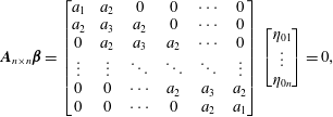(2.9)$$\begin{eqnarray}\displaystyle \boldsymbol{A}_{n\times n}\unicode[STIX]{x1D737}=\left[\begin{array}{@{}cccccc@{}}a_{1} & a_{2} & 0 & 0 & \cdots \, & 0\\ a_{2} & a_{3} & a_{2} & 0 & \cdots \, & 0\\ 0 & a_{2} & a_{3} & a_{2} & \cdots \, & 0\\ \vdots & \vdots & \ddots & \ddots & \ddots & \vdots \\ 0 & 0 & \cdots \, & a_{2} & a_{3} & a_{2}\\ 0 & 0 & \cdots \, & 0 & a_{2} & a_{1}\end{array}\right]\left[\begin{array}{@{}c@{}}\unicode[STIX]{x1D702}_{01}\\ \vdots \\ \unicode[STIX]{x1D702}_{0n}\end{array}\right]=0, & & \displaystyle\end{eqnarray}$$

(2.10)$$\begin{eqnarray}\displaystyle \left.\begin{array}{@{}c@{}}\displaystyle a_{1}=-\frac{\unicode[STIX]{x1D714}^{2}}{M_{S}}+U_{0}^{\ast -2}k^{4}-\frac{1+\coth (kd^{\ast })}{k}(\unicode[STIX]{x1D714}+k)^{2},\\ \displaystyle a_{2}=\frac{\text{csch}(kd^{\ast })}{k}(\unicode[STIX]{x1D714}+k)^{2},\\ \displaystyle a_{3}=-\frac{\unicode[STIX]{x1D714}^{2}}{M_{S}}+U_{0}^{\ast -2}k^{4}-\frac{2\coth (kd^{\ast })}{k}(\unicode[STIX]{x1D714}+k)^{2},\end{array}\right\} & & \displaystyle\end{eqnarray}$$

where $d^{\ast }=d/L$.

On the basis of the solution identification theorem in linear equations, $\left|\boldsymbol{A}_{n\times n}\right|$ must be equal to 0, that is

(2.11)$$\begin{eqnarray}\displaystyle \left|\begin{array}{@{}cccccc@{}}a_{1} & a_{2} & 0 & 0 & \cdots \, & 0\\ a_{2} & a_{3} & a_{2} & 0 & \cdots \, & 0\\ 0 & a_{2} & a_{3} & a_{2} & \cdots \, & 0\\ \vdots & \vdots & \ddots & \ddots & \ddots & \vdots \\ 0 & 0 & \cdots \, & a_{2} & a_{3} & a_{2}\\ 0 & 0 & \cdots \, & 0 & a_{2} & a_{1}\end{array}\right|=0. & & \displaystyle\end{eqnarray}$$

The coupled flapping mode of every two parallel inverted flags depends on

(2.12)$$\begin{eqnarray}\displaystyle \frac{\unicode[STIX]{x1D702}_{0l}}{\unicode[STIX]{x1D702}_{0m}}=G\text{e}^{\text{i}\unicode[STIX]{x1D703}_{lm}},\quad l,m=1,2,\ldots n. & & \displaystyle\end{eqnarray}$$

Here, $G$ and $\unicode[STIX]{x1D703}_{lm}$ are the ratios of the amplitude and phase angle, respectively. When $\unicode[STIX]{x1D703}_{lm}=0$ or $\unicode[STIX]{x03C0}$, the two inverted flags are in the in-phase or anti-phase flapping modes, respectively.

3.1 Force and energy distributions

Taking $U_{0}^{\ast }=2.88$ as an example, figure 3 shows the periodic oscillation of the free end over time based on the experimental data, where the circles and curve correspond to the experimental and fitting results, respectively. The equation of this curve is $y(t)=0.8L\sin (2\unicode[STIX]{x03C0}\times 0.13t+\unicode[STIX]{x1D711}_{0})$, where $0.8L$ is the amplitude, 0.13 is the flapping frequency and $\unicode[STIX]{x1D711}_{0}$ is the initial phase at $t=0$. The other positions along the inverted flag also have similar fitting results, and there is no phase difference between the different positions. When the initial phase $\unicode[STIX]{x1D711}_{0}=0$, the spanwise oscillation of the inverted flag can be approximately described as

(3.1)$$\begin{eqnarray}\displaystyle y(s,t)=A(s)\sin (2\unicode[STIX]{x03C0}f_{\unicode[STIX]{x1D714}}t), & & \displaystyle\end{eqnarray}$$

where $s$ is the curve coordinate from the fixed end to the free end, $A(s)$ is the amplitude at different positions and $f_{\unicode[STIX]{x1D714}}$ is the flapping frequency.

Figure 3. Variation of the tip spanwise displacement at $U_{0}^{\ast }=2.88$, where the circles and the curve represent the experimental and fitting results, respectively.

For $U_{0}^{\ast }=2.88$, $A(s)=-1.2162\times 10^{3}s^{5}+722.5s^{4}-153.4s^{3}+15.53s^{2}+0.17s$. Then, the spanwise oscillation of the inverted flag can be described as

(3.2)$$\begin{eqnarray}y(s,t)=(-1.2162\times 10^{3}s^{5}+722.5s^{4}-153.4s^{3}+15.53s^{2}+0.17s)\sin (2\unicode[STIX]{x03C0}\times 0.13t).\end{eqnarray}$$

In addition, the streamwise oscillation of the inverted flag can be obtained by $(\unicode[STIX]{x2202}x/\unicode[STIX]{x2202}s)^{2}+(\unicode[STIX]{x2202}y/\unicode[STIX]{x2202}s)^{2}=1$.

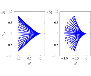
A comparison of the fitting and experimental results is shown in figure 4. Figures 4(a) and 4(b) present the spanwise displacement at each point and the dynamic profiles of the inverted flag, respectively, where $s^{\ast }=s/L$, $x^{\ast }=x/L$ and $y^{\ast }=y/L$. The left-hand panel of each pair shows the fitting results, and the right-hand panel the experimental results. The results obtained by the above method are in good agreement with the experimental results.

Figure 4. A comparison of the fitting and experimental results of the flag profiles at $U_{0}^{\ast }=2.88$: (a) spanwise displacement at each point along the inverted flag; (b) dynamic profiles of the inverted flag. The left-hand and right-hand panels of each pair represent the fitting and experimental results, respectively.

After obtaining the oscillation equation of the inverted flag, the force and energy distributions at different times can be further statistically analysed. Referring to Jia & Yin (Reference Jia and Yin2008), the equations for the force and energy distributions of a two-dimensional flag are as follows:

(3.3)$$\begin{eqnarray}\displaystyle & \displaystyle \left.\begin{array}{@{}c@{}}\displaystyle f_{1}=B\frac{\unicode[STIX]{x2202}^{4}y}{\unicode[STIX]{x2202}s^{4}},\\ \displaystyle f_{2}=\unicode[STIX]{x1D70C}_{s}h\frac{\unicode[STIX]{x2202}^{2}y}{\unicode[STIX]{x2202}t^{2}},\\ \displaystyle f_{y}=f_{1}+f_{2},\end{array}\right\} & \displaystyle\end{eqnarray}$$

(3.4)$$\begin{eqnarray}\displaystyle & \displaystyle \left.\begin{array}{@{}c@{}}\displaystyle e_{p}(s,t)=\frac{B}{2}\frac{(\unicode[STIX]{x2202}^{2}y/\unicode[STIX]{x2202}s^{2})^{2}}{1-(\unicode[STIX]{x2202}y/\unicode[STIX]{x2202}s)^{2}},\\ \displaystyle e_{k}(s,t)=\frac{\unicode[STIX]{x1D70C}_{s}h}{2}\left[\left(\frac{\unicode[STIX]{x2202}x}{\unicode[STIX]{x2202}t}\right)^{2}+\left(\frac{\unicode[STIX]{x2202}y}{\unicode[STIX]{x2202}t}\right)^{2}\right],\\ \displaystyle e(s,t)=e_{p}(s,t)+e_{k}(s,t).\end{array}\right\} & \displaystyle\end{eqnarray}$$

Here, $f_{1}$, $f_{1}$ and $f_{y}$ are the elastic force, inertia force and total distributed force in the $y$ direction, respectively; and $e_{p}$, $e_{k}$ and $e$ are the strain energy, kinetic energy and total distributed energy, respectively.

The force and energy distributions for a representative case of $U_{0}^{\ast }=2.88$ are given below. Figure 5 shows the variation of the force distribution and the tip displacement over a period. Figure 5(a) presents the distribution of the elastic force $f_{1}$ in one cycle, corresponding to the force that causes the flag to be bent. It can be determined that the elastic force $f_{1}$ reaches a maximum at the fixed end $(s^{\ast }=0)$ of the inverted flag, gradually decreases along the flag and is mainly concentrated in the range $0\leqslant s^{\ast }\leqslant 0.5$. Thus, the bending of the inverted flag is mainly concentrated near the fixed end. Since the elastic force $f_{1}$ causes the flag to bend, the elastic force $f_{1}$ at different positions and the tip displacement present the same trend over time. During the periods 0–$0.25T$ and $0.5T$–$0.75T$, the inverted flag is in the bending process. The larger the displacement of the flag, the larger the elastic force $f_{1}$. During the periods $0.25T$–$0.5T$ and $0.75T$–$T$, the inverted flag is in the rebounding process. The displacement and elastic force $f_{1}$ then gradually decrease. The above results show that the elastic force $f_{1}$ reaches a minimum at the equilibrium position (i.e. $t/T=0,0.5,1$) and a maximum at the leftmost or rightmost position (i.e. $t/T=0.25,0.75$).

Figure 5(b) displays the distribution of the inertia force $f_{2}$ in one cycle, corresponding to the force that causes the flag to oscillate. In contrast to the elastic force $f_{1}$, the inertia force $f_{2}$ gradually increases along the flag and is the largest at the free end $(s^{\ast }=1)$ of the inverted flag. This phenomenon is mainly because the acceleration of the flag can be calculated from the oscillation equation (3.1) as $-4\unicode[STIX]{x03C0}^{2}{f_{\unicode[STIX]{x1D714}}}^{2}A(s)\sin (2\unicode[STIX]{x03C0}f_{\unicode[STIX]{x1D714}}t)$, resulting in the maximum acceleration at the free end of the inverted flag. It also causes an opposite trend of the inertia force $f_{2}$ and the tip displacement.

By comparing figures 5(a) and 5(b), it can be determined that the elastic force $f_{1}$ is approximately $10^{3}$ times the inertia force $f_{2}$. Although the trends of these two types of forces are opposite over time, the trends and magnitudes of the distributed force $f_{y}$ are almost the same as those of the elastic force $f_{1}$, as shown in figure 5(c). This is explainable because the distributed force $f_{y}$ of the inverted flag is mainly completely provided by the elastic force $f_{1}$ during the oscillation process.

Figure 5. Variation of the force distribution in a period: (a) the elastic force $f_{1}$ ($\text{N}~\text{m}^{-1}$), (b) the inertia force $f_{2}$ ($\text{N}~\text{m}^{-1}$) and (c) the distributed force $f_{y}=f_{1}+f_{2}$ ($\text{N}~\text{m}^{-1}$). (d) Variation of the tip displacement in a period.

Figure 6 shows the variation of the energy distribution and the tip displacement over a period. Figures 6(a) and 6(b) present the distributions of the strain energy $e_{p}$ and the kinetic energy $e_{k}$, respectively. Figure 6(c) gives the energy distribution $e=e_{p}+e_{k}$ in one cycle. From figures 5(a) and 6(a), it is determined that the trend of the strain energy $e_{p}$ along the flag is the same as that of the elastic force $f_{1}$, both of which gradually decrease along the flag due to the maximum degree of bending of the fixed end. According to the expression of $e_{p}$ in (3.4), the strain energy $e_{p}$ at different positions and the absolute value of the tip displacement show the same trend over time. Given that the velocity of the flag can be written as $2\unicode[STIX]{x03C0}f_{\unicode[STIX]{x1D714}}A(s)\cos (2\unicode[STIX]{x03C0}f_{\unicode[STIX]{x1D714}}t)$, the kinetic energy $e_{k}$ gradually decreases along the flag, and a phase difference of 0.25T occurs between it and the absolute value of the tip displacement (see figure 6b,d). Similar to that shown in figure 5, the strain energy $e_{p}$ is also approximately $10^{3}$ times the kinetic energy $e_{k}$. Thus, the trends of the distributed energy $e$ and the strain energy $e_{p}$ are almost identical.

Both figures 5 and 6 show that the elastic component (i.e. $f_{1}$ and $e_{p}$) is several orders of magnitude greater than the inertia component (i.e. $f_{2}$ and $e_{k}$). In contrast, these two components of a conventional flag are of the same magnitude (Jia Reference Jia2009). This is mainly because the flag stiffness required for the large-amplitude flapping of the inverted flag is several orders of magnitude larger than that of the conventional flag under the same conditions. Additionally, the elastic component of the conventional flag is concentrated near the free end because its tip bends the most (Jia Reference Jia2009), which is contrary to the results for the inverted flag in our study.

Figure 6. Variation in the energy distribution in a period: (a) the strain energy $e_{p}$ ($\text{J}~\text{m}^{-1}$), (b) the kinetic energy $e_{k}$ ($\text{J}~\text{m}^{-1}$) and (c) the distributed energy $e=e_{p}+e_{k}$ ($\text{J}~\text{m}^{-1}$). (d) Variation of the displacement of the tip in a period.

The force and energy distributions in figures 5 and 6 are integrated along the flag, and then the variation in the total force and total energy in one cycle can be obtained. Figures 7(a) and 7(b) give the time history of the total force $F_{y}$ in the $y$ direction and the total energy $E$ in one cycle, respectively. As shown in figures 5(c) and 7(a), the trend of $F_{y}$ is similar to that of the distributed force $f_{y}$. This phenomenon is mainly because the distributed force $f_{y}$ has the same trend at different positions (see figure 5c). Specifically, $F_{y}$ of the inverted flag is constantly increasing during the bending process, and in the rebound process $F_{y}$ decreases continuously. As depicted in figures 6(c) and 7(b), the trends of the total energy E and the distributed energy e are also identical. The total energy E continues to increase during the bending process, corresponding to the energy accumulation process. In other words, the inverted flag collects energy from the surrounding fluid in the bending process. Additionally, the trend of the total energy E is opposite in the rebounding process, corresponding to the energy release process. Under this condition, the inverted flag releases energy into the surrounding fluid through the leading-edge vortex.

Figure 7. Variation of (a) the total force $F_{y}$ (N) in the y direction and (b) the total energy E (J) in a period.

The time-averaged energy $\overline{E}=(1/T)\int _{0}^{T}E\,\text{d}t$ of the inverted flag can be further evaluated. The conversion ratio, defined as $R=E_{\max }/E_{f}$ (Kim et al. Reference Kim, Cossé, Huertas-Cerdeira and Gharib2013; Ryu et al. Reference Ryu, Park, Kim and Sung2015), represents the efficiency of energy harvesting from the fluid kinetic energy to the flag strain energy; $E_{f}=0.5\unicode[STIX]{x1D70C}_{f}U_{0}^{3}A$ is the kinetic energy of the uniform flow in which $E_{max}$ the strain energy at the maximum deformation position, and $A$ is the amplitude of the inverted flag. Figure 8 shows the time-averaged energy $\overline{E}$, the amplitude A and the conversion ratio R at different flow velocities. In addition, the critical velocities between the straight, flapping and deflected modes are marked by dashed lines. For the definition of these three modes, see Hu et al. (Reference Hu, Wang, Wang and Breitsamter2019). It is determined from figure 8(a) that the trend of the time-averaged energy $\overline{E}$ is essentially consistent with that of the amplitude $A/L$ as a function of the flow velocity, indicating that the amplitude of the inverted flag gives a good estimate of the strain energy. The present results further reveal that the averaged energy $\overline{E}$ in the deflected mode is equivalent to that in the flapping mode. As shown in figure 8(b), the conversion ratio R first increases and then decreases with the successive increase in the flow velocity. The maximum conversion ratio R immediately follows the critical velocity, which is earlier than for the experimental results of Kim et al. (Reference Kim, Cossé, Huertas-Cerdeira and Gharib2013) in a wind tunnel. Unlike the averaged energy $\overline{E}$ plotted in figure 8(a), the conversion ratio R of the deflected mode is far lower than that of the flapping mode.

Figure 8. Variation in (a) the average energy $\overline{E}$ and amplitude $A/L$ and (b) conversion ratio R at different flow velocities.

3.2 Linear analysis

The force and energy distributions of an isolated inverted flag during the oscillation process are analysed above. It can be concluded that the averaged energy and conversion ratio are considerable in the flapping mode. Hence, it is of great significance to determine the critical velocities between the different modes. To achieve this goal, a theoretical analysis provides us with a more convenient but sufficiently accurate approach in comparison with the experimental means. Thus, a theoretical analysis is further conducted to reveal the characteristics of the critical velocities. To give a global overview, isolated and multiple inverted flags will be analysed.

For the linear stability analysis of an isolated inverted flag ($n=1$), equation (2.11) can be written as

(3.5)$$\begin{eqnarray}\displaystyle (\unicode[STIX]{x1D714}+k)^{2}+\left(\frac{k\unicode[STIX]{x1D714}^{2}}{M_{S}}-U_{0}^{\ast -2}k^{5}\right)/2=0. & & \displaystyle\end{eqnarray}$$

The imaginary part $\pm \unicode[STIX]{x1D714}_{i}$ of the complex frequency $\unicode[STIX]{x1D714}$ corresponds to the growth rate of disturbance. When $\unicode[STIX]{x1D714}_{i}>0$ the inverted flag is unstable. To investigate the effect of $M_{S}$ and $U_{0}^{\ast }$ on the dynamic behaviour of the inverted flag, the wavenumber k must first be determined. For a cantilever beam with one end fixed and one end free, the wavenumbers of the first three modes are $k=1.875$, 4.694 and 7.855, respectively (Young & Felgar Reference Young and Felgar1949). Substituting the wavenumbers of the first three modes into (3.5), the critical flow velocities can be obtained (see the curves in figure 9). The critical flow velocities obtained from previous experiments (Kim et al. Reference Kim, Cossé, Huertas-Cerdeira and Gharib2013; Fan Reference Fan2015; Sader et al. Reference Sader, Cossé, Kim, Fan and Gharib2016) and theoretical results (based on Kim & Kim (Reference Kim and Kim2019)) are also shown in figure 9. It can be determined that the critical flow velocities obtained from the experiments are located around the theoretical curve of wavenumber $k=1.875$, especially at a small mass ratio. This is mainly because the value of $\unicode[STIX]{x1D714}$ in (3.5) is indeed almost zero for a small mass ratio, which is similar to the result of assuming $\unicode[STIX]{x1D714}=0$ by Kim & Kim (Reference Kim and Kim2019). This further explains the applicability of the above theoretical model for a small mass ratio. For an isolated conventional flag, however, the critical flow velocity corresponds to the wavenumber of the second mode $k=4.694$ (Schouveiler & Eloy Reference Schouveiler and Eloy2009). Thus, although there is a great difference between inverted and conventional flags, the applicability of this theoretical model to an isolated inverted flag is acceptable.

Figure 9. The curves represent the critical flow velocities of an isolated inverted flag at different wavenumbers k, and the symbols represent the results of previous experiments.

However, figure 9 also shows that for large mass ratios, the critical velocity obtained in our experiment is much larger than that of the theoretical results of Kim & Kim (Reference Kim and Kim2019). Additionally, the discrepancy between our experimental and theoretical results can reach an order of magnitude. Specifically, the critical velocity obtained in our experiment is $U_{0}^{\ast }=2.7$; in contrast, the result predicted by the theoretical model is 33.6, and the result based on Kim & Kim (Reference Kim and Kim2019) is 1.815. The reasons for the discrepancies are as follows. The experiments in previous studies (Kim et al. Reference Kim, Cossé, Huertas-Cerdeira and Gharib2013; Yu et al. Reference Yu, Liu and Chen2017, Reference Yu, Liu and Chen2018; Chen et al. Reference Chen, Yu, Zhou, Peng and Liu2018) using a water tunnel yielded a single-side small-amplitude flapping mode (i.e. a biased mode). When $\unicode[STIX]{x1D714}=0$ is assumed, the critical velocity obtained in the above condition is the critical velocity at which the biased mode, rather than the large-amplitude flapping mode, begins to occur. Without assuming $\unicode[STIX]{x1D714}=0$, the static divergence instability is not satisfied, resulting in an excessive prediction result. Additionally, the same degree of discrepancy was also found by Shelley et al. (Reference Shelley, Vandenberghe and Zhang2005) for a conventional flag at large mass ratios due to the ignoring of the viscous force in (2.3). The viscous force has a diverging effect for the inverted flag, thus leading to a larger prediction result (see figure 9). In contrast, the viscous force causes the conventional flag to be stable, and thus a smaller prediction result was found (Shelley et al. Reference Shelley, Vandenberghe and Zhang2005). To reduce the effect of the viscous force and improve the reliability of (2.3), an additional experiment was performed on a special inverted flag with five steel sheets attached on each surface; thus, the mass ratio is reduced to $M_{S}=106$. The results show that the critical velocity is then increased to 3.96, which is significantly improved compared to the critical velocity of 2.7, and becomes closer to the results of the theoretical prediction. However, the critical velocity at which a large-amplitude oscillation disappears does not change. This indicates that the mass ratio has a certain impact on the critical velocity for the water tunnel experiments.

In conclusion, although the oscillation of the inverted flag is caused by static divergent instability, the mass ratio can affect the critical velocity to some extent in a water tunnel, and $\unicode[STIX]{x1D714}$ is almost zero in a wind tunnel. Therefore, unlike Kim & Kim (Reference Kim and Kim2019), while we do not directly assume $\unicode[STIX]{x1D714}=0$, the above results are highly reliable. As shown below, the theoretical model is mainly applied to inverted flags at small mass ratios.

To further verify the practicality of the theoretical model for inverted flags at small mass ratios, we compare the theoretical and experimental results for two parallel inverted flags. For the linear stability analysis of two inverted flags ($n=2$), four solutions of the complex frequency $\unicode[STIX]{x1D714}$ in (2.11) can be obtained for determined $d^{\ast }$, $M_{S}$ and $U_{0}^{\ast }$. The imaginary parts $\unicode[STIX]{x1D714}_{1i}$ obtained by $a_{1}-a_{2}=0$ indicate that the two inverted flags are in the anti-phase flapping mode since $G=1$ and $\unicode[STIX]{x1D703}_{12}=\unicode[STIX]{x03C0}$ (see (2.12)). Similarly, the imaginary part $\unicode[STIX]{x1D714}_{2i}$ obtained by $a_{1}+a_{2}=0$ indicates that the two inverted flags are in the in-phase flapping mode since $G=1$ and $\unicode[STIX]{x1D703}_{12}=0$ (see (2.12)). When $\unicode[STIX]{x1D714}_{1i}>0$ or $\unicode[STIX]{x1D714}_{2i}>0$, the two inverted flags begin to oscillate. The coupled flapping mode depends on the relative sizes of $\unicode[STIX]{x1D714}_{1i}$ and $\unicode[STIX]{x1D714}_{2i}$. Therefore, the definition of the disturbance growth rate ratio $\unicode[STIX]{x1D6FE}$ is as follows:

(3.6)$$\begin{eqnarray}\displaystyle \unicode[STIX]{x1D6FE}=\frac{\unicode[STIX]{x1D714}_{2i}}{\unicode[STIX]{x1D714}_{1i}}. & & \displaystyle\end{eqnarray}$$

Figure 10 shows the statistical analysis of the disturbance growth rate ratio $\unicode[STIX]{x1D6FE}$ in the ($M_{S}$, $U_{0}^{\ast }$)-plane under different separation distances. The $\unicode[STIX]{x1D6FE}<1$ region corresponds to the anti-phase flapping mode (region II). The $\unicode[STIX]{x1D6FE}>1$ region corresponds to the in-phase flapping mode (region III). The $\unicode[STIX]{x1D6FE}=1$ region corresponds to the indefinite flapping mode (region IV), in which the coupled flapping mode cannot be determined. The solid line corresponds to the critical flow velocity where the two parallel inverted flags convert between different modes. As shown in figure 10, two inverted flags are both in the straight mode (region I) at a low flow velocity. As the flow velocity increases, the two inverted flags enter the anti-phase flapping mode and finally enter the in-phase flapping mode, which is consistent with the experimental results in a wind tunnel (Huertas-Cerdeira et al. Reference Huertas-Cerdeira, Fan and Gharib2018). When $d^{\ast }\approx 0$, the two inverted flags can be regarded as one inverted flag. In this case, the two inverted flags always oscillate in phase (see figure 10a). As presented in figure 10(b–d), region III (the in-phase flapping mode) becomes smaller, and the disturbance growth rate ratio $\unicode[STIX]{x1D6FE}$ in region II becomes closer to 1. When $d^{\ast }=4$, the indefinite flapping mode (region IV) occurs. Additionally, the disturbance growth rate ratio $\unicode[STIX]{x1D6FE}$ is almost always 1 in region II or, to be exact, always larger than 0.999. Given the uncertainties in the experiments, the two inverted flags may enter a multiple flapping state dominated by the anti-phase flapping mode under this condition.

Figure 10. Contour plot denoting the disturbance growth rate ratio $\unicode[STIX]{x1D6FE}$ in the ($M_{S},U_{0}^{\ast }$)-plane under different separation distances: (a) $d^{\ast }=0.0001$, (b) $d^{\ast }=1$, (c) $d^{\ast }=2$ and (d) $d^{\ast }=4$. Region I corresponds to the straight mode ($\unicode[STIX]{x1D6FE}$ is not a number); II corresponds to the anti-phase flapping mode ($\unicode[STIX]{x1D6FE}<1$); III corresponds to the in-phase flapping mode ($\unicode[STIX]{x1D6FE}>1$); and IV corresponds to the indefinite mode ($\unicode[STIX]{x1D6FE}=1$).

Figure 11 presents the results of the theoretical analysis for two inverted flags with different disturbances but a fixed mass ratio of 0.42, with the experimental results of the in-phase and anti-phase flapping modes from the previous experiment of Huertas-Cerdeira et al. (Reference Huertas-Cerdeira, Fan and Gharib2018) also being given. The thin solid curve in region II represents $\unicode[STIX]{x1D6FE}=0.99$. The theoretical analysis shows that the in-phase flapping mode (region III) only occurs at small separation distances. With an increase in the flap distance, the in-phase flapping mode disappears, and the anti-phase flapping mode (region II) occurs. In general, the present predicted critical velocities for the anti-phase flapping mode are quite close to the experimental data. In region II, the disturbance growth rate ratio $\unicode[STIX]{x1D6FE}$ first decreases rapidly before gradually increasing. When $d^{\ast }>2$, the disturbance growth rate ratio $\unicode[STIX]{x1D6FE}$ begins to be greater than 0.99, which is denoted as the region to the right of the thin solid curve. Under this condition, the perturbation growth rates of the in-phase and anti-phase flapping modes are almost the same, and the two inverted flags may enter a multiple flapping state. Therefore, the critical velocities obtained from the experiment in which the anti-phase oscillation begins to disappear are located near $\unicode[STIX]{x1D6FE}=0.99$. It can be concluded that the inviscid model presents a good estimate of the critical velocities between the different flapping modes and explains the occurrence of multiple flapping states at a mass ratio of approximately 1, fully indicating the good applicability, easy operability and high reliability of the theoretical model for two parallel inverted flags.

Figure 11. Contour plot denoting the disturbance growth rate ratio $\unicode[STIX]{x1D6FE}$ in the ($d^{\ast },U_{0}^{\ast }$)-plane at $M_{S}=0.42$. The definitions of regions I, II, III and IV are presented in figure 10. Symbols ▴ (in-phase) and ○ (anti-phase) represent the experimental results in a wind tunnel $(M_{S}=0.42)$ conducted by Huertas-Cerdeira et al. (Reference Huertas-Cerdeira, Fan and Gharib2018).

Figure 12. (a) Observation of the coupled flapping modes of $n=3$ and $d^{\ast }=2$: $\unicode[STIX]{x1D702}_{01}/\unicode[STIX]{x1D702}_{03}=1$, $\unicode[STIX]{x1D702}_{02}/\unicode[STIX]{x1D702}_{03}=-p_{31}$ (mode 1); $\unicode[STIX]{x1D702}_{01}/\unicode[STIX]{x1D702}_{03}=1$, $\unicode[STIX]{x1D702}_{02}/\unicode[STIX]{x1D702}_{03}=p_{32}$ (mode 2); and $\unicode[STIX]{x1D702}_{01}/\unicode[STIX]{x1D702}_{03}=-1$, $\unicode[STIX]{x1D702}_{02}=0$ (mode 3). (b) Observation of the coupled flapping modes of $n=4$ and $d^{\ast }=2$: $\unicode[STIX]{x1D702}_{01}/\unicode[STIX]{x1D702}_{04}=-1$, $\unicode[STIX]{x1D702}_{02}/\unicode[STIX]{x1D702}_{03}=-1$, $\unicode[STIX]{x1D702}_{01}/\unicode[STIX]{x1D702}_{02}=-p_{41}$ (mode 1); $\unicode[STIX]{x1D702}_{01}/\unicode[STIX]{x1D702}_{04}=1$, $\unicode[STIX]{x1D702}_{02}/\unicode[STIX]{x1D702}_{03}=1$, $\unicode[STIX]{x1D702}_{01}/\unicode[STIX]{x1D702}_{02}=p_{42}$ (mode 2); $\unicode[STIX]{x1D702}_{01}/\unicode[STIX]{x1D702}_{04}=-1$, $\unicode[STIX]{x1D702}_{02}/\unicode[STIX]{x1D702}_{03}=-1$, $\unicode[STIX]{x1D702}_{01}/\unicode[STIX]{x1D702}_{02}=p_{43}$ (mode 3); and $\unicode[STIX]{x1D702}_{01}/\unicode[STIX]{x1D702}_{04}=1$, $\unicode[STIX]{x1D702}_{02}/\unicode[STIX]{x1D702}_{03}=1$, $\unicode[STIX]{x1D702}_{01}/\unicode[STIX]{x1D702}_{02}=-p_{44}$ (mode 4).

Since the results of the theoretical model are in good agreement with the experimental results of a single and two inverted flags at small mass ratios, it can be concluded that this model has a certain practicability for studying the oscillation of inverted flags at small mass ratios. Then, we extend two flags to $n>2$ flags in order to study the coupled flapping modes of multiple inverted flags. For $n>2$ inverted flags, the method of determining the coupled flapping mode is similar to that for the two inverted flags (see (2.11) and (2.12)). Figure 12 shows the critical velocities at which the different flapping modes begin to occur in the $(M_{S},U_{0}^{\ast })$-plane for $n=3$ and 4 and $d^{\ast }=2$. When $n=3$, three flapping modes are predicted by the theoretical model: $\unicode[STIX]{x1D702}_{01}/\unicode[STIX]{x1D702}_{03}=1$, $\unicode[STIX]{x1D702}_{02}/\unicode[STIX]{x1D702}_{03}=-p_{31}$ (mode 1); $\unicode[STIX]{x1D702}_{01}/\unicode[STIX]{x1D702}_{03}=1$, $\unicode[STIX]{x1D702}_{02}/\unicode[STIX]{x1D702}_{03}=p_{32}$ (mode 2); and $\unicode[STIX]{x1D702}_{01}/\unicode[STIX]{x1D702}_{03}=-1$, $\unicode[STIX]{x1D702}_{02}=0$ (mode 3). Here $p_{31}$ and $p_{32}$ are two positive coefficients that are only related to $M_{S}$ and $U_{0}^{\ast }$. When $n=4$, four flapping modes are predicted by the theoretical model: $\unicode[STIX]{x1D702}_{01}/\unicode[STIX]{x1D702}_{04}=-1$, $\unicode[STIX]{x1D702}_{02}/\unicode[STIX]{x1D702}_{03}=-1$, $\unicode[STIX]{x1D702}_{01}/\unicode[STIX]{x1D702}_{02}=-p_{41}$ (mode 1); $\unicode[STIX]{x1D702}_{01}/\unicode[STIX]{x1D702}_{04}=1$, $\unicode[STIX]{x1D702}_{02}/\unicode[STIX]{x1D702}_{03}=1$, $\unicode[STIX]{x1D702}_{01}/\unicode[STIX]{x1D702}_{02}=p_{42}$ (mode 2); $\unicode[STIX]{x1D702}_{01}/\unicode[STIX]{x1D702}_{04}=-1$, $\unicode[STIX]{x1D702}_{02}/\unicode[STIX]{x1D702}_{03}=-1$, $\unicode[STIX]{x1D702}_{01}/\unicode[STIX]{x1D702}_{02}=p_{43}$ (mode 3); and $\unicode[STIX]{x1D702}_{01}/\unicode[STIX]{x1D702}_{04}=1$, $\unicode[STIX]{x1D702}_{02}/\unicode[STIX]{x1D702}_{03}=1$, $\unicode[STIX]{x1D702}_{01}/\unicode[STIX]{x1D702}_{02}=-p_{44}$ (mode 4). Here $p_{41}$, $p_{42}$, $p_{43}$ and $p_{44}$ are four positive coefficients related to $M_{S}$ and $U_{0}^{\ast }$. It can be determined that only two kinds of flapping modes are observed under most parameters at $n=3$ and 4. Additionally, several other flapping modes are concentrated in only a small parameter range. Similarly, for $n=5$, 6 and 7 inverted flags, the theoretical model predicts 6, 8 and 12 coupled flapping modes, respectively. By analogy, when $n=2q$ ($q\geqslant 1$), the theoretical model predicts $2^{q}$ coupled flapping modes; when $n=2q+1,2^{q}+2^{(q-1)}$ coupled flapping modes are predicted by the theoretical model.