


1 Introduction
A centrepiece in the theory of inviscid shear flow is the classical critical level, where the phase speed  $c$ of a steady wave matches the local mean-flow speed
  $U$. In linear theory, the levels where
  $c=U$ become singular, demanding the inclusion of the weak effects of unsteadiness, nonlinearity or viscosity (Maslowe Reference Maslowe1986). Although these inclusions can remove the singularity of the linear inviscid theory, perturbations to the flow can still develop strongly in the neighbourhood of the critical levels, creating distinctive flow structures and rearrangements within the so-called critical layers that may subsequently break down to generate mixing and turbulence. In this vein, Warn & Warn (Reference Warn and Warn1976, Reference Warn and Warn1978) and Stewartson (Reference Stewartson1978) studied the nonlinear dynamics of the critical layers of forced Rossby waves. They found that steady waves developed over the bulk of the shear flow, but that the critical layer remained unsteady, exciting mean-flow corrections and all the harmonics of the original wavenumber, and twisting up the background vorticity into a Kelvin cat’s eye pattern. A similar scenario exists for the critical layers of internal gravity waves travelling vertically through stratified shear flow, with important repercussions on wave breaking, momentum transport and mixing in the atmosphere (Booker & Bretherton Reference Booker and Bretherton1967; Brown & Stewartson Reference Brown and Stewartson1980, Reference Brown and Stewartson1982a,Reference Brown and Stewartsonb).
If the flow is stratified vertically but sheared horizontally, then a new type of critical level appears in the linear inviscid wave theory. The new critical levels arise along the surfaces where the phase speed relative to the background shear flow matches a characteristic velocity of gravity waves; i.e.  $c-U=\pm N/k$, where
  $N$ is the buoyancy frequency and
  $k$ is the streamwise wavenumber. Existing literature on these ‘baroclinic critical levels’, has mainly focused on the propagation of linear wave packets. Using ray-tracing theory, Olbers (Reference Olbers1981), Basovich & Tsimring (Reference Basovich and Tsimring1984) and Badulin, Shrira & Tsimring (Reference Badulin, Shrira and Tsimring1985) found that wave packets slow down as they approach the baroclinic critical level, never reaching it. Simultaneously, the wave amplitude and cross-stream wavenumber grow indefinitely, indicating that linear theory eventually fails in a wave-trapping process like that found earlier for classical critical levels (Bretherton Reference Bretherton1966). Staquet & Huerre (Reference Staquet and Huerre2002) and Edwards & Staquet (Reference Edwards and Staquet2005) performed numerical simulations to study the nonlinear evolution during trapping, concluding that the trapped waves may either break into small-scale turbulence or be dissipated by dispersion, viscosity and diffusion. More related to the current work is the study by Boulanger, Meunier & Le Dizès (Reference Boulanger, Meunier and Le Dizès2007), who explored the analogues of baroclinic critical levels in stratified, titled vortices, and resolved the resulting singularities by introducing viscosity.
Baroclinic critical layers have also featured heavily in recently reported computations of three-dimensional rotating stratified shear flows with self-replicating vortices (Marcus et al. Reference Marcus, Pei, Jiang and Barranco2015, Reference Marcus, Pei, Jiang and Barranco2016; Barranco, Pei & Marcus Reference Barranco, Pei and Marcus2018). The replication process involves the forcing of baroclinic critical layers by internal waves excited by an initial vortex; large-amplitude re-arrangements forced in these layers then roll up to create new vortices, which in turn shed more internal waves to repeat a cycle. The self-replication eventually filled the computational domain with localized vortical structures, which was suggested to be trigger for the angular momentum transport required to drive accretion in astrophysical disks that are too cool to suffer the magneto-rotational instability.
The aim of the present paper is to theoretically study the evolution of forced baroclinic critical layers, following the paradigm of Stewartson (Reference Stewartson1978) and Warn & Warn (Reference Warn and Warn1976, Reference Warn and Warn1978) for Rossby waves, or Booker & Bretherton (Reference Booker and Bretherton1967) and Brown & Stewartson (Reference Brown and Stewartson1980, Reference Brown and Stewartson1982a,Reference Brown and Stewartsonb) for internal waves in stratified shear flow. The linear dynamics of a forced baroclinic critical layer is expected to be similar to that of a classical critical layer, owing to the similarity of the singularities in the linear wave equations. However, the subsequent nonlinear evolution is likely to be very different because the location of the baroclinic critical level itself is dictated by the streamwise wavenumber, which is different among all the harmonics of the original wave. This suggests that they cannot feature in the nonlinear dynamics within the baroclinic critical layer, unlike in classical critical-layer theory.
The layout of the paper is as follows: in § 2, we give the model and governing equations of the problem. In § 3, we solve the linear problem explicitly and draw out structure that first develops within the baroclinic critical layer. In § 4, we extend the analysis by considering weakly nonlinear perturbations, which allows us to determine the time and length scales that characterize the nonlinear critical layer. This leads us, in § 5, to derive a reduced model of nonlinear dynamics via a matched asymptotic expansion. We then present numerical solutions of the reduced model and a further asymptotic analysis of them. We explore the effects of dissipation in the baroclinic critical layer in § 6, and then discuss the implications of the results and the relation to previous and future work in § 7.
2 Model and governing equations
We consider forced disturbances to an unbounded horizontal shear flow, orientated in the  $x$-direction with a constant shear rate
  $\unicode[STIX]{x1D6EC}>0$ in the
  $y$-direction. The domain rotates around the vertical axis at angular velocity
  $\unicode[STIX]{x1D6FA}$, and the fluid is stratified in
  $z$ with constant buoyancy frequency
  $N$. Waves are driven into the shear flow by a wavemaker that we locate along
  $y=0$. This forcing has the streamwise and vertical wavenumbers,
  $k_{x}$ and
  $k_{z}$, respectively. The baroclinic critical levels are located at
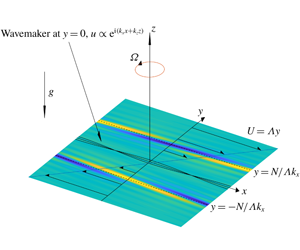
  $y=\pm N/(\unicode[STIX]{x1D6EC}k_{x})$. The sketch of the model is shown in figure 1.

Figure 1. Sketch of the model. A wavemaker with wavenumbers  $k_{x}$ and
  $k_{z}$ is imposed at
  $y=0$, and baroclinic critical levels are forced at
  $y=\pm N/(\unicode[STIX]{x1D6EC}k_{x})$, corresponding to dimensionless locations
  $\pm {\mathcal{N}}$, where
  ${\mathcal{N}}=N\unicode[STIX]{x1D6EC}^{-1}$. The shading represents a rendering of the density perturbation based on the linear theory of § 3.
We work with a dimensionless version of the governing fluid equations in which length, time, velocity, pressure and density perturbations are scaled by  $k_{x}^{-1}$,
  $\unicode[STIX]{x1D6EC}^{-1}$,
  $\unicode[STIX]{x1D6EC}k_{x}^{-1}$,
  $\unicode[STIX]{x1D70C}_{0}\unicode[STIX]{x1D6EC}^{2}k_{x}^{-2}$ and
  $\unicode[STIX]{x1D70C}_{0}\unicode[STIX]{x1D6EC}^{2}/(k_{x}g)$, respectively. Here,
  $\unicode[STIX]{x1D70C}_{0}$ is a reference density and
  $g$ is gravity. We employ the Boussinesq approximation and, for the most part of our study, neglect viscosity and diffusion in view of the large spatial scales that characterize geophysical and astrophysical flows. At the end of the work, we briefly explore the effect of diffusion. The perturbations to the velocity
  $(u,v,w)$, pressure
  $p$ and perturbation density
  $\unicode[STIX]{x1D70C}$ then satisfy
 $$\begin{eqnarray}\displaystyle & \displaystyle u_{t}+yu_{x}+(1-f)v+uu_{x}+vu_{y}+wu_{z}=-p_{x}, & \displaystyle\end{eqnarray}$$
 $$\begin{eqnarray}\displaystyle & \displaystyle v_{t}+yv_{x}+fu+uv_{x}+vv_{y}+wv_{z}=-p_{y}, & \displaystyle\end{eqnarray}$$
 $$\begin{eqnarray}\displaystyle & \displaystyle w_{t}+yw_{x}+uw_{x}+vw_{y}+ww_{z}=-p_{z}-\unicode[STIX]{x1D70C}, & \displaystyle\end{eqnarray}$$
 $$\begin{eqnarray}\displaystyle & \displaystyle \unicode[STIX]{x1D70C}_{t}+y\unicode[STIX]{x1D70C}_{x}-{\mathcal{N}}^{2}w+u\unicode[STIX]{x1D70C}_{x}+v\unicode[STIX]{x1D70C}_{y}+w\unicode[STIX]{x1D70C}_{z}=0, & \displaystyle\end{eqnarray}$$
 $$\begin{eqnarray}\displaystyle & \displaystyle u_{x}+v_{y}+w_{z}=0, & \displaystyle\end{eqnarray}$$
 where subscripts represent partial derivatives and we have introduced the dimensionless Coriolis parameter  $f=2\unicode[STIX]{x1D6FA}/\unicode[STIX]{x1D6EC}$ and buoyancy frequency
  ${\mathcal{N}}=N\unicode[STIX]{x1D6EC}^{-1}$. Because our interest lies in the forcing of the baroclinic critical layers of an internal wave, we consider basic flows that are linearly stable to prevent unstable modes from dominating the dynamics. Centrifugal instabilities arise when
  $0<f<1$ (Emanuel Reference Emanuel1994), so we set
  $f>1$ or
  $f<0$ to eliminate them; strato-rotational instability is not present because it requires reflective boundaries (Yavneh, McWilliams & Molemaker Reference Yavneh, McWilliams and Molemaker2001; Wang & Balmforth Reference Wang and Balmforth2018) which are absent here.
Initially, there is no disturbance, implying  $u=v=w=\unicode[STIX]{x1D70C}=p=0$ at
  $t=0$. The wavemaker is then switched on to excite waves with baroclinic critical levels. To idealize the forcing and formulate a concise mathematical problem, we assume that the wavemaker introduces a time-independent jump in the tangential horizontal velocity at
  $y=0$, but not in the normal velocity. That is, we impose the jump conditions,
 $$\begin{eqnarray}\displaystyle u|_{y=0+}-u|_{y=0-}=\unicode[STIX]{x1D700}_{0}\exp (\text{i}\,x+\text{i}mz)+\text{c.c.},\quad v|_{y=0+}=v|_{y=0-}, & & \displaystyle\end{eqnarray}$$
 where  $\unicode[STIX]{x1D700}_{0}$ represents the strength,
  $m=k_{z}/k_{x}$, c.c. represents the complex conjugate, and the
  $\pm$ superscripts indicate the limits from either side. This forcing approximates a thin, spatially periodic vortex sheet. In the numerical simulation of Marcus et al. (Reference Marcus, Pei, Jiang and Hassanzadeh2013), waves were forced by a periodic array of localized Gaussian vortices. Our forcing therefore represents an idealization of their model in that we consider the leading-order Fourier component while neglecting the evolution and cross-stream thickness of the forcing. The configuration is slightly different to that in the studies of Stewartson (Reference Stewartson1978) and Booker & Bretherton (Reference Booker and Bretherton1967), where a wavy boundary forced the normal velocity. The current configuration implies that waves are generated at
  $y=0$ and develop with baroclinic critical levels to either side (although simplifications are afforded by the symmetry described presently). Had we placed the wavemaker along a boundary at
  $y=0$, only one critical level would have featured, but the wall may also make the basic flow linearly unstable (Wang & Balmforth Reference Wang and Balmforth2018). Other idealizations include wavemakers that gradually switch on (Béland Reference Béland1976) or have finite thickness (as for the vortices of Marcus et al.), or that generate disturbances with finite phase speed (displacing the baroclinic critical levels).
Note that the system in (2.1)–(2.6) is invariant under the transformation,
 $$\begin{eqnarray}\displaystyle (u,v,w,\unicode[STIX]{x1D70C})\rightarrow -(u,v,w,\unicode[STIX]{x1D70C})\quad \text{and}\quad p\rightarrow p,\quad \text{for }(x,y,z)\rightarrow -(x,y,z).\quad & & \displaystyle\end{eqnarray}$$
 This observation permits us to solve the problem only for  $y>0$, and we therefore consider only one baroclinic critical layer and then generate the solution in
  $y<0$ using the implied symmetry conditions.
Also, combining (2.1)–(2.5), we may derive an equation for the vertical component of vorticity,
 $$\begin{eqnarray}\displaystyle \frac{\text{D}}{\text{D}t}(v_{x}-u_{y})-{\mathcal{N}}^{-2}(f-1+v_{x}-u_{y})\frac{\unicode[STIX]{x2202}}{\unicode[STIX]{x2202}z}\frac{\text{D}\unicode[STIX]{x1D70C}}{\text{D}t}+w_{x}v_{z}-w_{y}u_{z}=0, & & \displaystyle\end{eqnarray}$$
where
 $$\begin{eqnarray}\displaystyle \frac{\text{D}}{\text{D}t}=\frac{\unicode[STIX]{x2202}}{\unicode[STIX]{x2202}t}+(y+u)\frac{\unicode[STIX]{x2202}}{\unicode[STIX]{x2202}x}+v\frac{\unicode[STIX]{x2202}}{\unicode[STIX]{x2202}y}+w\frac{\unicode[STIX]{x2202}}{\unicode[STIX]{x2202}z}. & & \displaystyle\end{eqnarray}$$
3 Linear theory
The linearized governing equations are
 $$\begin{eqnarray}\displaystyle & \displaystyle u_{t}+yu_{x}+(1-f)v=-p_{x}, & \displaystyle\end{eqnarray}$$
 $$\begin{eqnarray}\displaystyle & \displaystyle v_{t}+yv_{x}+fu=-p_{y}, & \displaystyle\end{eqnarray}$$
 $$\begin{eqnarray}\displaystyle & \displaystyle w_{t}+yw_{x}+\unicode[STIX]{x1D70C}=-p_{z}, & \displaystyle\end{eqnarray}$$
 $$\begin{eqnarray}\displaystyle & \displaystyle \unicode[STIX]{x1D70C}_{t}+y\unicode[STIX]{x1D70C}_{x}-{\mathcal{N}}^{2}w=0, & \displaystyle\end{eqnarray}$$
 $$\begin{eqnarray}\displaystyle & \displaystyle u_{x}+v_{y}+w_{z}=0. & \displaystyle\end{eqnarray}$$
 The linearized equation of (2.8) reduces to a conservation law of potential vorticity,  $q_{t}+yq_{x}=0$, or, given that
  $q=0$ everywhere at
  $t=0$,
 $$\begin{eqnarray}\displaystyle q=(f-1)\unicode[STIX]{x1D70C}_{z}-{\mathcal{N}}^{2}(v_{x}-u_{y})=0. & & \displaystyle\end{eqnarray}$$
In the absence of linear instability, the forcing (2.6) drives a steady-wave response throughout the bulk of the flow (as can be established by solving the initial-value problem using Laplace transforms, and then performing a large-time asymptotic analysis, following Booker & Bretherton (Reference Booker and Bretherton1967) and Warn & Warn (Reference Warn and Warn1976)). Near the baroclinic critical levels, however, the flow remains unsteady, requiring a finer analysis of those regions similar to that used by Stewartson (Reference Stewartson1978).
3.1 The steady-wave response outside the baroclinic critical layers
The steady-wave solution outside the critical layers takes the form,
 $$\begin{eqnarray}\displaystyle (u,v,w,p,\unicode[STIX]{x1D70C})=[\hat{u} (y),\hat{v}(y),{\hat{w}}(y),\hat{p}(y),\hat{\unicode[STIX]{x1D70C}}(y)]\exp (\text{i}x+\text{i}mz)+\text{c.c.} & & \displaystyle\end{eqnarray}$$
 Substituting (3.7) into (3.1)–(3.5), one can derive an equation for  $\hat{p}(y)$,
 $$\begin{eqnarray}\displaystyle \hat{p}^{\prime \prime }-\frac{2y}{y^{2}-f(f-1)}\hat{p}^{\prime }-\left[\frac{y^{2}-f(f+1)}{y^{2}-f(f-1)}+m^{2}\frac{y^{2}-f(f-1)}{y^{2}-{\mathcal{N}}^{2}}\right]\hat{p}=0, & & \displaystyle\end{eqnarray}$$
with
 $$\begin{eqnarray}\displaystyle \hat{u} =\frac{(f-1)\hat{p}^{\prime }-y\hat{p}}{y^{2}-f(f-1)},\quad \hat{v}=\frac{\text{i}(y\hat{p}^{\prime }-f\hat{p})}{y^{2}-f(f-1)},\quad {\hat{w}}=-\frac{my\hat{p}}{y^{2}-{\mathcal{N}}^{2}},\quad \hat{\unicode[STIX]{x1D70C}}=\frac{\text{i}m{\mathcal{N}}^{2}\hat{p}}{y^{2}-{\mathcal{N}}^{2}} & & \displaystyle \nonumber\\ \displaystyle & & \displaystyle\end{eqnarray}$$
 (cf. Vanneste & Yavneh Reference Vanneste and Yavneh2007). Note that the singularities at  $y^{2}=f(f-1)$ in (3.8) and (3.9) are removable. The baroclinic critical levels
  $y=\pm {\mathcal{N}}$, however, are true singular points. The Frobenius solutions near
  $y={\mathcal{N}}$ are,
 $$\begin{eqnarray}\displaystyle & \displaystyle \hat{p}_{A}=1-\frac{m^{2}[{\mathcal{N}}^{2}-f(f-1)]}{2{\mathcal{N}}}({\mathcal{N}}-y)\log |{\mathcal{N}}-y|-\unicode[STIX]{x1D6FC}({\mathcal{N}}-y)+\cdots \,, & \displaystyle\end{eqnarray}$$
 $$\begin{eqnarray}\displaystyle & \displaystyle \hat{p}_{B}=y-{\mathcal{N}}+\cdots \,, & \displaystyle\end{eqnarray}$$
 where  $\unicode[STIX]{x1D6FC}$ is determined by the condition that
  $\hat{p}_{A}\rightarrow 0$ as
  $y\rightarrow \infty$. In terms of these Frobenius solutions, we express
  $\hat{p}$ for
  $y>0$ by
 $$\begin{eqnarray}\displaystyle \hat{p}=\left\{\begin{array}{@{}ll@{}}A_{L}\hat{p}_{A}, & y>{\mathcal{N}},\\ A_{L}\hat{p}_{A}+B_{L}\hat{p}_{B}, & 0<y<{\mathcal{N}},\end{array}\right. & & \displaystyle\end{eqnarray}$$
 where  $A_{L}$ and
  $B_{L}$ are constants.
Although  $\hat{p}$ is bounded for
  $y\rightarrow {\mathcal{N}}$, the amplitudes of the velocity,
  $(\hat{u} ,\hat{v},{\hat{w}})$, and density,
  $\hat{\unicode[STIX]{x1D70C}}$, all diverge, signifying that the steady-wave solution fails at the critical levels. In particular, we observe that
 $$\begin{eqnarray}\displaystyle \hat{p}\rightarrow A_{L},\quad \hat{\unicode[STIX]{x1D70C}}\rightarrow \frac{\text{i}m{\mathcal{N}}A_{L}}{2(y-{\mathcal{N}})} & & \displaystyle\end{eqnarray}$$
and
 $$\begin{eqnarray}\displaystyle \hat{u} & \rightarrow & \displaystyle \left[\frac{m^{2}(f-1)}{2{\mathcal{N}}}(\log |{\mathcal{N}}-y|+1)+\frac{\unicode[STIX]{x1D6FC}(f-1)-{\mathcal{N}}}{{\mathcal{N}}^{2}-f(f-1)}\right]A_{L}\nonumber\\ \displaystyle & & \displaystyle +\left\{\begin{array}{@{}ll@{}}0 & y>{\mathcal{N}},\\ \displaystyle \frac{f-1}{{\mathcal{N}}^{2}-f(f-1)}B_{L} & y<{\mathcal{N}},\end{array}\right.\end{eqnarray}$$
 for  $y\rightarrow {\mathcal{N}}$.
3.2 The linear critical layers
We now focus on the baroclinic critical layer at  $y={\mathcal{N}}$. Here, we search for an unsteady solution depending on the long time scale
  $T=\unicode[STIX]{x1D6FF}t$ and with the short spatial scale
  $Y=(y-{\mathcal{N}})/\unicode[STIX]{x1D6FF}$, where
  $\unicode[STIX]{x1D6FF}\ll 1$ is a small parameter organizing an asymptotic expansion. We then set
 $$\begin{eqnarray}\displaystyle (u,v,w,p,\unicode[STIX]{x1D70C})=[\widetilde{u}(Y,T),\widetilde{v}(Y,T),\unicode[STIX]{x1D6FF}^{-1}\widetilde{w}(Y,T),A_{L},\unicode[STIX]{x1D6FF}^{-1}\widetilde{\unicode[STIX]{x1D70C}}(Y,T)]\exp (\text{i}x+\text{i}mz)+\text{c.c.}, & & \displaystyle \nonumber\\ \displaystyle & & \displaystyle\end{eqnarray}$$
in view of the limits in (3.13)–(3.14).
Combining (3.3) and (3.4) to eliminate  $w$, then substituting in (3.15) now gives, to leading order in
  $\unicode[STIX]{x1D6FF}$,
 $$\begin{eqnarray}\displaystyle \left(\frac{\unicode[STIX]{x2202}}{\unicode[STIX]{x2202}T}+\text{i}Y\right)\widetilde{\unicode[STIX]{x1D70C}}=-\frac{1}{2}m{\mathcal{N}}A_{L}. & & \displaystyle\end{eqnarray}$$
 In the early stage of linear evolution,  $t\sim O(1)$,
  $\unicode[STIX]{x1D70C}\sim O(1)$, so we have the initial condition
  $\widetilde{\unicode[STIX]{x1D70C}}\rightarrow 0$ as
  $T\rightarrow 0$, which yields
 $$\begin{eqnarray}\displaystyle \widetilde{\unicode[STIX]{x1D70C}}=-\frac{1}{2}\text{i}m{\mathcal{N}}A_{L}\frac{\text{e}^{-\text{i}YT}-1}{Y}. & & \displaystyle\end{eqnarray}$$
Hence
 $$\begin{eqnarray}\displaystyle \unicode[STIX]{x1D70C}=-\frac{1}{2}\text{i}m{\mathcal{N}}A_{L}t\left[\frac{\text{e}^{-\text{i}(y-{\mathcal{N}})t}-1}{(y-{\mathcal{N}})t}\right]\text{e}^{\text{i}x+\text{i}mz}+\text{c.c.} & & \displaystyle\end{eqnarray}$$
 This solution has a spatial structure dependent on the self-similar combination  $t(y-{\mathcal{N}})$. Hence, the amplitude grows linearly and the width of the critical layer shrinks with time.
Next, the main balance in (3.6) implies that  $\widetilde{u}_{Y}\sim -\text{i}m(f-1){\mathcal{N}}^{-2}\widetilde{\unicode[STIX]{x1D70C}}$, or
 $$\begin{eqnarray}\displaystyle \widetilde{u}_{Y}=-\frac{m^{2}(f-1)A_{L}}{2{\mathcal{N}}}\frac{\text{e}^{-\text{i}YT}-1}{Y}. & & \displaystyle\end{eqnarray}$$
 But the limits of the steady-wave response in (3.14) imply that  $\widetilde{u}$ jumps by an amount
  $(f-1)B_{L}/[{\mathcal{N}}^{2}-f(f-1)]$ across the baroclinic critical layer. Hence,
 $$\begin{eqnarray}\displaystyle B_{L}=-\frac{m^{2}A_{L}[f(f-1)-{\mathcal{N}}^{2}]}{2{\mathcal{N}}}\lim _{L\rightarrow \infty }\int _{-L}^{L}(\text{e}^{-\text{i}YT}-1)\frac{\text{d}Y}{Y}=\text{i}\unicode[STIX]{x03C0}\frac{m^{2}[f(f-1)-{\mathcal{N}}^{2}]}{2{\mathcal{N}}}A_{L} & & \displaystyle \nonumber\\ \displaystyle & & \displaystyle\end{eqnarray}$$
(cf. Stewartson Reference Stewartson1978).
3.3 Closure
We can now apply the forcing condition to close the problem. The symmetry property (2.7) applied to the steady wave (3.7) indicates that
 $$\begin{eqnarray}\displaystyle [\hat{u} (y),\hat{v}(y),{\hat{w}}(y),\hat{\unicode[STIX]{x1D70C}}(y)]=-[\hat{u} (-y),\hat{v}(-y),{\hat{w}}(-y),\hat{\unicode[STIX]{x1D70C}}(-y)]^{\ast },\quad \hat{p}(y)=\hat{p}(-y)^{\ast },\quad & & \displaystyle\end{eqnarray}$$
 where the superscript  $^{\ast }$ represents the complex conjugate. Hence, substituting the steady-wave solution into the jump condition (2.6) representing the forcing, we arrive at
 $$\begin{eqnarray}\displaystyle \left.\begin{array}{@{}c@{}}(A_{L}-A_{L}^{\ast })\hat{p}_{A}(0)+(B_{L}-B_{L}^{\ast })\hat{p}_{B}(0)=0,\\ (A_{L}+A_{L}^{\ast })\hat{p}_{A}^{\prime }(0)+(B_{L}+B_{L}^{\ast })\hat{p}_{B}^{\prime }(0)=-f\unicode[STIX]{x1D700}_{0}.\end{array}\right\} & & \displaystyle\end{eqnarray}$$
Exploiting (3.20), we obtain
 $$\begin{eqnarray}\displaystyle A_{L}=-\left.\frac{f\unicode[STIX]{x1D700}_{0}(\,\hat{p}_{A}-\text{i}\unicode[STIX]{x1D6FD}\hat{p}_{B})}{2(\,\hat{p}_{A}\hat{p}_{A}^{\prime }+\unicode[STIX]{x1D6FD}^{2}\hat{p}_{B}\hat{p}_{B}^{\prime })}\right|_{y=0},\quad \unicode[STIX]{x1D6FD}=\frac{\unicode[STIX]{x03C0}m^{2}[f(f-1)-{\mathcal{N}}^{2}]}{2{\mathcal{N}}}. & & \displaystyle\end{eqnarray}$$
The amplitude of the pressure perturbation at the critical layer is therefore
 $$\begin{eqnarray}\displaystyle \left.\unicode[STIX]{x1D700}=|A_{L}|=\frac{|\,f\unicode[STIX]{x1D700}_{0}|\sqrt{\hat{p}_{A}^{2}+\unicode[STIX]{x1D6FD}^{2}\hat{p}_{B}^{2}}}{2|\hat{p}_{A}\hat{p}_{A}^{\prime }+\unicode[STIX]{x1D6FD}^{2}\hat{p}_{B}\hat{p}_{B}^{\prime }|}\right|_{y=0}. & & \displaystyle\end{eqnarray}$$
A sample steady-wave solution is plotted in figure 2.

Figure 2. Steady-wave solution  $\hat{p}$ under a forcing imposed at
  $y=0$, with
  $m=0.5$,
 ${\mathcal{N}}=4/3$,
  $f=4/3$,
  $\unicode[STIX]{x1D700}_{0}=0.05$ (cf. Marcus et al. Reference Marcus, Pei, Jiang and Hassanzadeh2013). Baroclinic critical levels
  $y=\pm {\mathcal{N}}$ are indicated.
Note that equations (3.22)–(3.24) appear to become trivial if  $f=0$, suggesting that rotation is essential to the forcing of the baroclinic critical layer. In fact, a deeper analysis of the Frobenius solutions demonstrates that this is not the case, because
  $\hat{p}_{A}^{\prime }(0)$ and
  $\hat{p}_{B}^{\prime }(0)$ become
  $O(f)$ in this limit, and the closure relation in (3.22) remains non-trivial. Consequently, in the model, we may take the limit
  $f\rightarrow 0$, highlighting how rotation is not an essential ingredient to the dynamics.
The same feature does not apply to the vertical wavenumber or stratification, which control the secular growth inside the critical layer, as seen in (3.17) and (3.19); without either a vertical dependence in the forcing or stratification, there is no baroclinic critical-layer dynamics. Note that, despite appearances, the limit  ${\mathcal{N}}\rightarrow 0$ in (3.19) is not problematic: further analysis of
  $\hat{p}_{A}$ and
  $\hat{p}_{B}$ indicates that
  $|A_{L}|\sim {\mathcal{N}}/\log {\mathcal{N}}$ for
  ${\mathcal{N}}\rightarrow 0$, and so the secular growth in the critical layer is eliminated in this limit.
It is also noteworthy that, in the limit that any of the parameters  $m$,
$m$,  $f$ or
  ${\mathcal{N}}$ are large, the disturbance decays exponentially from the forcing to the baroclinic critical levels (cf. Vanneste & Yavneh (Reference Vanneste and Yavneh2007) and Wang & Balmforth (Reference Wang and Balmforth2018)). The amplitude ratio
  $\unicode[STIX]{x1D700}/\unicode[STIX]{x1D700}_{0}$ then becomes exponentially small, and the secular growth in the critical layer is much weakened.
4 The weakly nonlinear critical layer
We now advance beyond linear theory and perform a weakly nonlinear expansion by setting
 $$\begin{eqnarray}\displaystyle & & \displaystyle (u,v,w,\unicode[STIX]{x1D70C},p)=\unicode[STIX]{x1D700}\{[u_{1}(Y,T),v_{1}(Y,T),\unicode[STIX]{x1D6FF}^{-1}w_{1}(Y,T),\unicode[STIX]{x1D6FF}^{-1}\unicode[STIX]{x1D70C}_{1}(Y,T),p_{1}(Y,T)]\text{e}^{\text{i}x+\text{i}mz}+\text{c.c.}\}\nonumber\\ \displaystyle & & \displaystyle \quad +\,\unicode[STIX]{x1D700}^{2}[u_{0}(Y,T),v_{0}(Y,T),w_{0}(Y,T),\unicode[STIX]{x1D70C}_{0}(Y,T),p_{0}(Y,T)]\nonumber\\ \displaystyle & & \displaystyle \quad +\,\unicode[STIX]{x1D700}^{2}\{[u_{2}(Y,T),v_{2}(Y,T),w_{2}(Y,T),\unicode[STIX]{x1D70C}_{2}(Y,T),p_{2}(Y,T)]\text{e}^{2(\text{i}x+\text{i}mz)}+\text{c.c.}\},\end{eqnarray}$$
 focussing upon the critical layer with  $y={\mathcal{N}}+\unicode[STIX]{x1D6FF}Y$. The scaling of the fundamental Fourier component follows the linear critical-layer theory outlined above, and we have
  $\unicode[STIX]{x1D700}[u_{1},v_{1},w_{1},\unicode[STIX]{x1D70C}_{1},p_{1}]\rightarrow [\widetilde{u},\widetilde{v},\widetilde{w},\widetilde{\unicode[STIX]{x1D70C}},A_{L}]$ at early times (
 $T\ll 1$). The goal of the current section is to identify the time scale and width of the critical layer (as dictated by the small parameter
  $\unicode[STIX]{x1D6FF}$) for which the mean-flow correction and first harmonic reach a sufficient strength to modify the evolution of the fundamental mode. This connects
  $\unicode[STIX]{x1D6FF}$ to the amplitude parameter
  $\unicode[STIX]{x1D700}$, establishing the scalings of the nonlinear critical layer.
4.1 Mean-flow response
The mean-flow component of (2.5) gives  $v_{0Y}=0$, which implies
  $v_{0}=0$ since the mean-flow response decays outside the critical layer. The streamwise mean-flow velocity
  $u_{0}$ is described by the
  $j=0$ component of (2.1), which is
 $$\begin{eqnarray}\displaystyle \frac{\unicode[STIX]{x2202}u_{0}}{\unicode[STIX]{x2202}T}=\unicode[STIX]{x1D6FF}^{-2}(\text{i}mw_{1}u_{1}^{\ast }-v_{1}^{\ast }u_{1Y})+\text{c.c.} & & \displaystyle\end{eqnarray}$$
 To leading order in  $\unicode[STIX]{x1D6FF}$, the mean-flow components of (2.3) and (2.4) are,
 $$\begin{eqnarray}\displaystyle & \displaystyle \unicode[STIX]{x1D70C}_{0}=-\unicode[STIX]{x1D6FF}^{-2}v_{1}^{\ast }w_{1Y}+\text{c.c.}, & \displaystyle\end{eqnarray}$$
 $$\begin{eqnarray}\displaystyle & \displaystyle -{\mathcal{N}}^{2}w_{0}=-\unicode[STIX]{x1D6FF}^{-2}(v_{1}^{\ast }\unicode[STIX]{x1D70C}_{1Y}+\text{i}mw_{1}^{\ast }\unicode[STIX]{x1D70C}_{1})+\text{c.c.} & \displaystyle\end{eqnarray}$$
 Thus,  $u_{0}$,
  $w_{0}$ and
  $\unicode[STIX]{x1D70C}_{0}$ are all
  $O(\unicode[STIX]{x1D6FF}^{-2})$.
4.2 First harmonic
The largest first harmonic components of (2.3), (2.4), (2.5) and (2.8) indicate that
 $$\begin{eqnarray}\displaystyle & \displaystyle 2\text{i}\,{\mathcal{N}}w_{2}+\unicode[STIX]{x1D70C}_{2}+2\text{i}mp_{2}=-\unicode[STIX]{x1D6FF}^{-2}(v_{1}w_{1Y}+\text{i}mw_{1}^{2}), & \displaystyle\end{eqnarray}$$
 $$\begin{eqnarray}\displaystyle & \displaystyle 2\text{i}\,{\mathcal{N}}\unicode[STIX]{x1D70C}_{2}-{\mathcal{N}}^{2}w_{2}=-\unicode[STIX]{x1D6FF}^{-2}(v_{1}\unicode[STIX]{x1D70C}_{1Y}-\text{i}mw_{1}\unicode[STIX]{x1D70C}_{1}), & \displaystyle\end{eqnarray}$$
 $$\begin{eqnarray}\displaystyle & \displaystyle \unicode[STIX]{x1D6FF}^{-1}v_{2Y}+2\text{i}mw_{2}=0, & \displaystyle\end{eqnarray}$$
 $$\begin{eqnarray}\displaystyle & \displaystyle \frac{u_{2Y}}{\unicode[STIX]{x1D6FF}}+\frac{2\text{i}m(f-1)}{{\mathcal{N}}^{2}}\unicode[STIX]{x1D70C}_{2}=\frac{\text{i}\unicode[STIX]{x1D6FF}^{-2}}{2{\mathcal{N}}}\left[\frac{2\text{i}m(f-1)}{{\mathcal{N}}^{2}}(v_{1}\unicode[STIX]{x1D70C}_{1Y}+\text{i}mw_{1}\unicode[STIX]{x1D70C}_{1})+(v_{1}u_{1Y}+\text{i}mw_{1}u_{1})_{Y}\right]. & \displaystyle \nonumber\\ \displaystyle & & \displaystyle\end{eqnarray}$$
 However, equation (2.2) demands that  $p_{2}=O(\unicode[STIX]{x1D6FF}u_{2},\unicode[STIX]{x1D6FF}v_{2})$ and so
  $p_{2}$ is much smaller than
  $w_{2}$ or
  $\unicode[STIX]{x1D70C}_{2}$. Hence,
 $$\begin{eqnarray}\displaystyle & \displaystyle w_{2}=\frac{\unicode[STIX]{x1D6FF}^{-2}}{3{\mathcal{N}}^{2}}[2\text{i}\,{\mathcal{N}}(v_{1}w_{1Y}+\text{i}mw_{1}^{2})-v_{1}\unicode[STIX]{x1D70C}_{1Y}-\text{i}mw_{1}\unicode[STIX]{x1D70C}_{1}], & \displaystyle\end{eqnarray}$$
 $$\begin{eqnarray}\displaystyle & \displaystyle \unicode[STIX]{x1D70C}_{2}=\frac{\unicode[STIX]{x1D6FF}^{-2}}{3{\mathcal{N}}}[{\mathcal{N}}(v_{1}w_{1Y}+\text{i}mw_{1}^{2})+2\text{i}(v_{1}\unicode[STIX]{x1D70C}_{1Y}+\text{i}mw_{1}\unicode[STIX]{x1D70C}_{1})], & \displaystyle\end{eqnarray}$$
 which are  $O(\unicode[STIX]{x1D6FF}^{-2})$, whereas
  $u_{2}$ and
  $v_{2}$ are
  $O(\unicode[STIX]{x1D6FF}^{-1})$.
4.3 Weakly nonlinear feedback
On again combining (2.3) and (2.4), we find the fundamental components,
 $$\begin{eqnarray}\displaystyle \left(\frac{\unicode[STIX]{x2202}}{\unicode[STIX]{x2202}T}+\text{i}Y\right)\unicode[STIX]{x1D70C}_{1}+\frac{1}{2}m{\mathcal{N}}p_{1}=-\unicode[STIX]{x1D700}^{2}\unicode[STIX]{x1D6FF}^{-1}\text{i}u_{0}\unicode[STIX]{x1D70C}_{1}, & & \displaystyle\end{eqnarray}$$
 with the leading-order nonlinear terms included on the right, and after a considerable number of cancellations stemming from the use of (4.3), (4.4), (4.9) and (4.10) and the leading-order relations  $\unicode[STIX]{x1D70C}_{1}=-\text{i}\,{\mathcal{N}}w_{1}$ and
  $v_{1Y}=-\text{i}mw_{1}$. Note that the nonlinear terms generated by the first harmonic and mean-flow components
  $w_{0}$ and
  $\unicode[STIX]{x1D70C}_{0}$ completely cancel out at this stage, leaving only the effect of the modification to the streamwise mean flow
  $u_{0}$. But the scaling established for the mean-flow correction implies that the right-hand side of (4.11) is
  $O(\unicode[STIX]{x1D6FF}^{-3}\unicode[STIX]{x1D700}^{2})$. Thus, the mean flow feeds back on the fundamental mode when
  $\unicode[STIX]{x1D6FF}=\unicode[STIX]{x1D700}^{2/3}$. That is, for
 $$\begin{eqnarray}\displaystyle t=O(\unicode[STIX]{x1D700}^{-2/3}),\quad y={\mathcal{N}}+O(\unicode[STIX]{x1D700}^{2/3}). & & \displaystyle\end{eqnarray}$$
These are the scalings for the nonlinear critical-layer theory outlined in the next section.
Note that we may extend the analysis to consider the higher harmomics. One finds that when  $\unicode[STIX]{x1D6FF}=\unicode[STIX]{x1D700}^{2/3}$, the Fourier component
  $\text{e}^{\text{i}j(x+mz)}$ with
  $j>1$ is
  $O(\unicode[STIX]{x1D700}^{j/3})$, which signifies that the higher-order harmonics
  $j\geqslant 3$ are still weak when the mean-flow correction begins to feedback on the fundamental. Thus, the higher harmonics play no role in the nonlinear theory.
5 Nonlinear critical-layer theory
5.1 The reduction
Motivated by the weakly nonlinear analysis, we now introduce the rescalings,
 $$\begin{eqnarray}\displaystyle T=\unicode[STIX]{x1D700}^{2/3}t,\quad Y=\frac{y-{\mathcal{N}}}{\unicode[STIX]{x1D700}^{2/3}}. & & \displaystyle\end{eqnarray}$$
The outer solution for the pressure is
 $$\begin{eqnarray}\displaystyle p=\unicode[STIX]{x1D700}p_{1}\text{e}^{\text{i}(x+mz)}+\text{c.c.},\quad p_{1}=\left\{\begin{array}{@{}ll@{}}A(T)\hat{p}_{A}(y), & y>{\mathcal{N}},\\ A(T)\hat{p}_{A}(y)+B(T)\hat{p}_{B}(y), & 0<y<{\mathcal{N}},\end{array}\right. & & \displaystyle\end{eqnarray}$$
 which is a single dominant Fourier mode characterized by the steady-wave solution. However, the amplitudes  $A$ and
  $B$ now evolve with the slow time
  $T$, because the nonlinear evolution of the critical layer can affect the outer flow. Initially,
  $A$ and
  $B$ are given by the linear analysis,
 $$\begin{eqnarray}\displaystyle A(0)=\frac{A_{L}}{\unicode[STIX]{x1D700}},\quad B(0)=\frac{B_{L}}{\unicode[STIX]{x1D700}}. & & \displaystyle\end{eqnarray}$$
Inside the critical layers, we set
 $$\begin{eqnarray}\displaystyle \left.\begin{array}{@{}c@{}}p=\unicode[STIX]{x1D700}A(T)\text{e}^{\text{i}(x+mz)}+\text{c.c.}+\cdots \,,\quad [w,\unicode[STIX]{x1D70C}]=\unicode[STIX]{x1D700}^{1/3}[w_{1}(Y,T),\unicode[STIX]{x1D70C}_{1}(Y,T)]\text{e}^{\text{i}(x+mz)}+\text{c.c.}+\cdots \\ \hspace{0.0pt}[u,v]=\unicode[STIX]{x1D700}[u_{1}(Y,T),v_{1}(Y,T)]\text{e}^{\text{i}(x+mz)}\!+\text{c.c.}\!+\unicode[STIX]{x1D700}^{2/3}[U_{0}(Y,T),0]+\cdots \end{array}\right\}. & & \displaystyle \nonumber\\ \displaystyle & & \displaystyle\end{eqnarray}$$
Equation (4.11) and the leading-order fundamental-mode components of (2.1), (2.3)–(2.5) and (2.8) now become
 $$\begin{eqnarray}\displaystyle & \displaystyle \frac{\unicode[STIX]{x2202}\unicode[STIX]{x1D70C}_{1}}{\unicode[STIX]{x2202}T}+\text{i}Y\unicode[STIX]{x1D70C}_{1}+\frac{m{\mathcal{N}}}{2}A=-\text{i}U_{0}\unicode[STIX]{x1D70C}_{1}, & \displaystyle\end{eqnarray}$$
 $$\begin{eqnarray}\displaystyle & \displaystyle \text{i}\,{\mathcal{N}}u_{1}-(f-1)v_{1}+\text{i}A=-v_{1}U_{0Y}, & \displaystyle\end{eqnarray}$$
 $$\begin{eqnarray}\displaystyle w_{1}=\frac{\text{i}}{{\mathcal{N}}}\unicode[STIX]{x1D70C}_{1},\quad v_{1Y}=-\text{i}mw_{1}, & & \displaystyle\end{eqnarray}$$
 $$\begin{eqnarray}\displaystyle {\mathcal{N}}^{2}u_{1Y}+\text{i}m(f-1-U_{0Y})\unicode[STIX]{x1D70C}_{1}=\text{i}\,{\mathcal{N}}v_{1}U_{0YY}. & & \displaystyle\end{eqnarray}$$
 The initial condition of  $\unicode[STIX]{x1D70C}_{1}$ is given by the linear result
 $$\begin{eqnarray}\displaystyle \unicode[STIX]{x1D70C}_{1}\rightarrow -\frac{\text{i}m{\mathcal{N}}A(0)}{2}\frac{\text{e}^{-\text{i}YT}-1}{Y},\quad T\rightarrow 0. & & \displaystyle\end{eqnarray}$$
 Similar to (4.2), the mean-flow velocity  $U_{0}$ is governed by
 $$\begin{eqnarray}\displaystyle \frac{\unicode[STIX]{x2202}U_{0}}{\unicode[STIX]{x2202}T}=-v_{1}^{\ast }u_{1Y}+\text{i}mw_{1}u_{1}^{\ast }+\text{c.c.} & & \displaystyle\end{eqnarray}$$
 The initial condition is  $U_{0}\rightarrow 0$ as
  $T\rightarrow 0$, as in early linear evolution the mean-flow modification is minimal.
It is possible to algebraically manipulate (5.5)–(5.8) and then integrate in  $T$ to show that
 $$\begin{eqnarray}\displaystyle U_{0}=-\frac{2}{{\mathcal{N}}^{3}}|\unicode[STIX]{x1D70C}_{1}|^{2}, & & \displaystyle\end{eqnarray}$$
a result that can be traced back to the fact that the change to the mean flow is given by the Eulerian pseudo-momentum (Bühler Reference Bühler2014), which is the right-hand side of (5.11) to leading order in the critical layer. Hence
 $$\begin{eqnarray}\displaystyle \frac{\unicode[STIX]{x2202}\unicode[STIX]{x1D70C}_{1}}{\unicode[STIX]{x2202}T}+\text{i}Y\unicode[STIX]{x1D70C}_{1}+\frac{1}{2}m{\mathcal{N}}A=\text{i}\frac{2}{{\mathcal{N}}^{3}}|\unicode[STIX]{x1D70C}_{1}|^{2}\unicode[STIX]{x1D70C}_{1}. & & \displaystyle\end{eqnarray}$$
 To match the inner and outer solutions, we first note, from (5.7), that  $v_{1Y}=m{\mathcal{N}}^{-1}\unicode[STIX]{x1D70C}_{1}$. Integrating this relation in
  $Y$ over the critical layer then provides the jump of the outer solution
  $v_{1}=\text{i}(yp_{1,y}-fp_{1})/[y^{2}-f(f-1)]$ for the limit of
  $y\rightarrow {\mathcal{N}}$ (cf. (3.9b)), which yields
 $$\begin{eqnarray}\displaystyle B=-\text{i}m\frac{f(f-1)-{\mathcal{N}}^{2}}{{\mathcal{N}}^{2}}\int _{-\infty }^{\infty }\unicode[STIX]{x1D70C}_{1}\,\text{d}Y, & & \displaystyle\end{eqnarray}$$
in a similar manner to § 3.2 and (3.20).
Last, we again use the forcing condition at  $y=0$ to close the problem,
 $$\begin{eqnarray}\displaystyle \left.\begin{array}{@{}c@{}}(A-A^{\ast })\hat{p}_{A}(0)+(B-B^{\ast })\hat{p}_{B}(0)=0,\\ \displaystyle (A+A^{\ast })\hat{p}_{A}^{\prime }(0)+(B+B^{\ast })\hat{p}_{B}^{\prime }(0)=-f\frac{\unicode[STIX]{x1D700}_{0}}{\unicode[STIX]{x1D700}},\end{array}\right\} & & \displaystyle\end{eqnarray}$$
 (cf. § 3.3 and (3.22)). Note that the form of the forcing impacts the reduced model only through the closure relations in (5.14). Had we used a different idealization of the forcing here, there would be a different algebraic relation between  $A$,
$A$,  $B$ and
  $\unicode[STIX]{x1D700}_{0}/\unicode[STIX]{x1D700}$. However, this relation still connects
  $A$ with the forcing amplitude and the integral of
  $\unicode[STIX]{x1D70C}_{1}$ over the critical layer, and in the scaled, canonical system presented below, all that would change would be how the parameters of that system (denoted
  $c_{0}$,
  $c_{1}$ and
  $c_{2}$ in § 5.2) depend on the original physical constants. In this sense, the reduced model is independent of the choice of forcing.
5.2 Canonical system
The final rescalings
 $$\begin{eqnarray}\displaystyle \unicode[STIX]{x1D70C}_{1}=\left(\frac{m{\mathcal{N}}^{4}}{4}\right)^{1/3}\unicode[STIX]{x1D6FE}(\unicode[STIX]{x1D702},\unicode[STIX]{x1D70F}),\quad T=\left(\frac{2{\mathcal{N}}}{m^{2}}\right)^{1/3}\unicode[STIX]{x1D70F},\quad Y=\left(\frac{m^{2}}{2{\mathcal{N}}}\right)^{1/3}\unicode[STIX]{x1D702}, & & \displaystyle\end{eqnarray}$$
lead to the canonical form,
 $$\begin{eqnarray}\displaystyle & \displaystyle \frac{\unicode[STIX]{x2202}\unicode[STIX]{x1D6FE}}{\unicode[STIX]{x2202}\unicode[STIX]{x1D70F}}+\text{i}\unicode[STIX]{x1D702}\unicode[STIX]{x1D6FE}+A=\text{i}|\unicode[STIX]{x1D6FE}|^{2}\unicode[STIX]{x1D6FE}, & \displaystyle\end{eqnarray}$$
 $$\begin{eqnarray}\displaystyle & \displaystyle A(\unicode[STIX]{x1D70F})=c_{0}+\frac{\text{i}c_{1}}{\unicode[STIX]{x03C0}}\int _{-\infty }^{\infty }\unicode[STIX]{x1D6FE}_{r}\,\text{d}\unicode[STIX]{x1D702}-\frac{c_{2}}{\unicode[STIX]{x03C0}}\int _{-\infty }^{\infty }\unicode[STIX]{x1D6FE}_{i}\,\text{d}\unicode[STIX]{x1D702}, & \displaystyle\end{eqnarray}$$
 where  $\unicode[STIX]{x1D6FE}=\unicode[STIX]{x1D6FE}_{r}+\text{i}\unicode[STIX]{x1D6FE}_{i}$,
 $$\begin{eqnarray}\displaystyle c_{0}=-\text{sgn}\left(\frac{f}{\hat{p}_{A}^{\prime }(0)}\right)\frac{|1+c_{1}c_{2}|}{\sqrt{1+c_{1}^{2}}}, & & \displaystyle\end{eqnarray}$$
and
 $$\begin{eqnarray}\displaystyle \left\{\begin{array}{@{}c@{}}c_{1}\\ c_{2}\end{array}\right\}=\frac{\unicode[STIX]{x03C0}m^{2}[f(f-1)-{\mathcal{N}}^{2}]}{2{\mathcal{N}}}\left\{\begin{array}{@{}c@{}}\hat{p}_{B}(0)/\hat{p}_{A}(0)\\ \hat{p}_{B}^{\prime }(0)/\hat{p}_{A}^{\prime }(0)\end{array}\right\}. & & \displaystyle\end{eqnarray}$$
 For  $\unicode[STIX]{x1D70F}\ll 1$, we must match
  $\unicode[STIX]{x1D6FE}(\unicode[STIX]{x1D702},\unicode[STIX]{x1D70F})$ to the corresponding solution of the linear problem, given by
 $$\begin{eqnarray}\displaystyle \unicode[STIX]{x1D6FE}=\text{i}A\frac{1-\text{e}^{-\text{i}\unicode[STIX]{x1D702}\unicode[STIX]{x1D70F}}}{\unicode[STIX]{x1D702}},\quad A=\frac{c_{0}(1-\text{i}c_{1})}{1+c_{1}c_{2}}, & & \displaystyle\end{eqnarray}$$
which provides the initial condition for (5.16).
The reduced model equations in (5.16)–(5.20) are solved numerically in the next section. The system is integro-differential in the sense that (5.16) is an equation of motion in time, solved at each level of  $\unicode[STIX]{x1D702}$, with the integral constraint in (5.17). There is no dependence on either
  $x$ or
  $z$, because the leading-order dynamics involves only the fundamental mode of the forcing wave pattern and the mean-flow response (which is then prescribed by the pseudo-momentum). The only nonlinearity is the cubic term on the right of (5.16), which is generic in weakly nonlinear theories of non-dissipative systems with few degrees of freedom. The model is therefore rather different from those that emerge for classical forced critical layers, which usually take the form of partial differential equations in all the spatial variables. The reduced model has the two parameters,
  $c_{1}$ and
  $c_{2}$, and the choice of sign for
  $f\hat{p}_{A}^{\prime }(0)$ in
  $c_{0}$. In most situations
  $\hat{p}_{A}$ and
  $\hat{p}_{B}$ are characterized by a similar exponential away from
  $y=0$, implying
  $c_{1}\approx c_{2}$.
From (5.16)–(5.17), one can establish that the quantity,
 $$\begin{eqnarray}\displaystyle {\mathcal{H}}=\int _{-\infty }^{\infty }\left[\frac{1}{2}|\unicode[STIX]{x1D6FE}|^{4}-\unicode[STIX]{x1D702}|\unicode[STIX]{x1D6FE}|^{2}+2\text{Im}(A^{\ast }\unicode[STIX]{x1D6FE})\right]\text{d}\unicode[STIX]{x1D702}+\frac{c_{1}}{\unicode[STIX]{x03C0}}\left[\int _{-\infty }^{\infty }\unicode[STIX]{x1D6FE}_{r}\,\text{d}\unicode[STIX]{x1D702}\right]^{2}+\frac{c_{2}}{\unicode[STIX]{x03C0}}\left[\int _{-\infty }^{\infty }\unicode[STIX]{x1D6FE}_{i}\,\text{d}\unicode[STIX]{x1D702}\right]^{2}, & & \displaystyle \nonumber\\ \displaystyle & & \displaystyle\end{eqnarray}$$
 must be conserved, and therefore equal to  $\unicode[STIX]{x03C0}c_{1}(1+c_{1}c_{2})/(1+c_{1}^{2})$ in view of the initial conditions. This constraint implies that the linear-in-time growth of
  $\unicode[STIX]{x1D6FE}(\unicode[STIX]{x1D702},\unicode[STIX]{x1D70F})$ predicted by linear theory must eventually become arrested, as otherwise the quartic first term in (5.21) cannot be counter balanced by the remaining quadratic and constant terms. To determine the manner in which the arrest takes place, we turn to a numerical solution of the reduced model.
5.3 Numerical solutions
To solve the canonical system of equations numerically, we first select a grid in  $\unicode[STIX]{x1D702}$ spanning a finite domain (we use 1501 equally spaced grid points over the interval
  $1.5<\unicode[STIX]{x1D702}<3$ where
  $\unicode[STIX]{x1D6FE}$ has large gradients, then 1544 grid points distributed evenly over
  $-25<\unicode[STIX]{x1D702}<1.5$ and
  $3<\unicode[STIX]{x1D702}<25$). We then integrate (5.16) forward in time numerically using a fourth-order Runge–Kutta method at each of the grid points. To evaluate the integrals in (5.17), we use an approach similar to Warn & Warn (Reference Warn and Warn1978) to extrapolate the limits to infinity. We use parameter settings guided by the computations of Marcus et al. (Reference Marcus, Pei, Jiang and Hassanzadeh2013):
  $m=1/2$,
  $f=4/3$,
  ${\mathcal{N}}=4/3$, which yield
  $c_{1}=0.238$,
  $c_{2}=0.219$.
Figure 3 displays the evolution in  $\unicode[STIX]{x1D70F}$ of the forced wave amplitudes,
  $A$ and
  $B$, which is relatively mild with
  $\text{Re}(A)\approx c_{0}\approx -1$ and
  $\text{Im}(A)$,
  $\text{Re}(B)$ and
  $\text{Im}(B)$ all remaining small. This mild behaviour results because, in (5.17),
  $|c_{1}|$ and
  $|c_{2}|$ are fairly small. Thus, the forced wave evolves slowly over the bulk of the shear flow (i.e. the outer region), maintaining a profile similar to the linear distribution in figure 2.

Figure 3. Evolution of  $A$ and
  $B$ with
  $\unicode[STIX]{x1D70F}$;
  $m=1/2$,
  $f=4/3$,
  ${\mathcal{N}}=4/3$.

Figure 4. (a) Real and (b) imaginary parts of the critical-layer density perturbation  $\unicode[STIX]{x1D6FE}(\unicode[STIX]{x1D702},\unicode[STIX]{x1D70F})$, shown as surfaces above the
  $(\unicode[STIX]{x1D702},\unicode[STIX]{x1D70F})$-plane. To prevent the viewing perspective from obscuring parts of the solution, we also show density maps of the solutions underneath. The insets show corresponding plots of the linear solution in (5.20). Panels (c–f) plot snapshots of
  $\unicode[STIX]{x1D6FE}(\unicode[STIX]{x1D702},\unicode[STIX]{x1D70F})$ at the times indicated; the linear result for
  $|\unicode[STIX]{x1D6FE}(\unicode[STIX]{x1D702},\unicode[STIX]{x1D70F})|$ is also included. (
 $m=1/2$,
  $f=4/3$,
  ${\mathcal{N}}=4/3$.)
The density perturbation  $\unicode[STIX]{x1D6FE}(\unicode[STIX]{x1D702},\unicode[STIX]{x1D70F})$, shown in figure 4, exhibits a richer behaviour: for
  $\unicode[STIX]{x1D70F}<1$, the numerical solution follows the linear prediction in (5.20), with its characteristically developing undulations and linear growth near
  $\unicode[STIX]{x1D702}=0$ (see figure 4a,b). Once
  $|\unicode[STIX]{x1D701}|$ reaches order-one values there, however, the growth of the numerical solution saturates, as demanded by the constraint in (5.21). Despite this, the solution continues to undulate over increasingly shorter spatial scales. Moreover, nonlinear effects distort the density profile further, shifting the maximum magnitude from
  $\unicode[STIX]{x1D702}=0$ to a small, positive level in
  $\unicode[STIX]{x1D702}$ and generating pronounced fine structure over a narrow region nearby.
The rapid spatial variation in  $\unicode[STIX]{x1D6FE}(\unicode[STIX]{x1D702},\unicode[STIX]{x1D70F})$ significantly impacts the critical-layer vorticity, which depends on the
  $\unicode[STIX]{x1D702}$-derivatives of
  $\unicode[STIX]{x1D6FE}(\unicode[STIX]{x1D702},\unicode[STIX]{x1D70F})$. In particular, the leading-order vertical vorticity is given by the mean-flow vorticity
  $\unicode[STIX]{x1D701}_{0}$,
 $$\begin{eqnarray}\displaystyle \unicode[STIX]{x1D701}\sim \unicode[STIX]{x1D701}_{0}\equiv \frac{\unicode[STIX]{x2202}}{\unicode[STIX]{x2202}\unicode[STIX]{x1D702}}|\unicode[STIX]{x1D6FE}|^{2}. & & \displaystyle\end{eqnarray}$$
 However, from the matched asymptotic expansion, we may reconstruct  $\unicode[STIX]{x1D701}(x,\unicode[STIX]{x1D702},z,t)$ to higher orders, incorporating the fundamental Fourier mode
  $\unicode[STIX]{x1D701}_{1}$ and first harmonic
  $\unicode[STIX]{x1D701}_{2}$, as summarized in appendix A. The evolution of the reconstructed vertical vorticity field is plotted in figure 5. For early times,
  $\unicode[STIX]{x1D701}_{0}\ll 1$, and the vertical vorticity is actually given by the higher-order linear solution (as in figure 5a, cf. (3.19)). With the increase of
  $\unicode[STIX]{x1D70F}$, the vorticity distribution tilts over and
  $\unicode[STIX]{x1D701}_{0}$ grows to dominate
  $\unicode[STIX]{x1D701}$, as seen in figure 5(b,c). This growth leads to the distinctive dipolar stripe seen in figure 5(d). In the later stages of evolution (figure 5e,f), the stripe becomes stronger and more focussed, shifting slightly above
  $\unicode[STIX]{x1D702}=0$, and corresponding to the sharpening oscillations in
  $\unicode[STIX]{x1D6FE}$ seen in figure 4.

Figure 5. Snapshots of vertical vorticity  $\unicode[STIX]{x1D701}$ within the baroclinic critical layer near
  $y={\mathcal{N}}=4/3$, plotted as a colour map on the
  $(x,\unicode[STIX]{x1D702})$-plane for (a)
  $\unicode[STIX]{x1D70F}=0.3$, (b)
  $\unicode[STIX]{x1D70F}=0.45$, (c)
  $\unicode[STIX]{x1D70F}=0.6$, (d)
  $\unicode[STIX]{x1D70F}=1$, (e)
  $\unicode[STIX]{x1D70F}=1.5$ and (f)
  $\unicode[STIX]{x1D70F}=1.8$. The domain plotted is
  $|\unicode[STIX]{x1D702}|<25$, corresponding to
  $|y-{\mathcal{N}}|<0.39$, at cross-section
  $z=0$ and over one streamwise wavelength of the forcing pattern. (
 $\unicode[STIX]{x1D700}_{0}=0.05$,
  $\unicode[STIX]{x1D700}=0.0062$,
  $m=1/2$,
  $f=4/3$,
  ${\mathcal{N}}=4/3$.)
The behaviour of the numerical solution seen in figures 3–5 is generic for most parameter settings; for moderate  $m$,
$m$,  $f$ (either
  $f>1$ or
  $f<0$) and
  ${\mathcal{N}}$, the parameters
  $c_{1}$ and
  $c_{2}$ of the reduced model are relatively small in magnitude, prompting similar dynamics. Even when
  $|c_{1}|$ and
  $|c_{2}|$ become order one, the evolution still bears qualitative similarities. However, more complicated behaviour can occur in the reduced model when these parameters take higher values. Such parameter settings can be achieved at special combinations of
  $m$,
$m$,  $f$ and
  ${\mathcal{N}}$ for which
  $\hat{p}_{A}(0)$ becomes small, or perhaps for other types of forcing. We avoid consideration of special situations of this sort, and instead turn to a deeper analysis of the focussing dynamics observed in the reduced model.
5.4 Long-time focussing
In view of the result that  $A$ changes slowly, we now use the approximation of
  $A=\text{const.}$ to gain further analytical insights into the focussing phenomenon. This device was used previously by Stewartson (Reference Stewartson1978) to obtain an analytical solution to the nonlinear evolution of Rossby wave critical layers. In our model, constant
  $A$ in (5.17) requires
  $c_{1}=c_{2}=0$, hence
  $A=-\text{sgn}(f\hat{p}_{A}^{\prime }(0))$, which is
  $-1$ for the current parameter setting. The evolution equation (5.16) can then be written as the one-degree-of-freedom Hamiltonian system,
 $$\begin{eqnarray}\displaystyle \left.\begin{array}{@{}c@{}}\displaystyle \frac{\unicode[STIX]{x2202}\unicode[STIX]{x1D6FE}_{r}}{\unicode[STIX]{x2202}\unicode[STIX]{x1D70F}}=\frac{\unicode[STIX]{x2202}H}{\unicode[STIX]{x2202}\unicode[STIX]{x1D6FE}_{i}}=1+\unicode[STIX]{x1D702}\unicode[STIX]{x1D6FE}_{i}-\unicode[STIX]{x1D6FE}_{r}^{2}\unicode[STIX]{x1D6FE}_{i}-\unicode[STIX]{x1D6FE}_{i}^{3},\\ \displaystyle \frac{\unicode[STIX]{x2202}\unicode[STIX]{x1D6FE}_{i}}{\unicode[STIX]{x2202}\unicode[STIX]{x1D70F}}=-\frac{\unicode[STIX]{x2202}H}{\unicode[STIX]{x2202}\unicode[STIX]{x1D6FE}_{r}}=-\unicode[STIX]{x1D702}\unicode[STIX]{x1D6FE}_{r}+\unicode[STIX]{x1D6FE}_{r}^{3}+\unicode[STIX]{x1D6FE}_{r}\unicode[STIX]{x1D6FE}_{i}^{2},\end{array}\right\} & & \displaystyle\end{eqnarray}$$
with Hamiltonian,
 $$\begin{eqnarray}\displaystyle H=-{\textstyle \frac{1}{4}}(\unicode[STIX]{x1D6FE}_{r}^{2}+\unicode[STIX]{x1D6FE}_{i}^{2})^{2}+{\textstyle \frac{1}{2}}\unicode[STIX]{x1D702}(\unicode[STIX]{x1D6FE}_{r}^{2}+\unicode[STIX]{x1D6FE}_{i}^{2})+\unicode[STIX]{x1D6FE}_{i} & & \displaystyle\end{eqnarray}$$
 (the point-wise version of the conserved quantity  ${\mathcal{H}}$ in (5.21) for
  $c_{1}=c_{2}=0$). For the specific initial condition of our critical-layer problem,
  $H=0$ for all values of
  $\unicode[STIX]{x1D702}$.
Figure 6(a) illustrates the phase portrait of the system (5.23) for the special choice  $\unicode[STIX]{x1D702}=\unicode[STIX]{x1D702}_{c}=3/\sqrt[3]{2}$. In this case, the orbit from
  $(\unicode[STIX]{x1D6FE}_{r},\unicode[STIX]{x1D6FE}_{i})=(0,0)$ lies along a separatrix that converges to a saddle point at
  $(\unicode[STIX]{x1D6FE}_{r},\unicode[STIX]{x1D6FE}_{i})=(0,-\unicode[STIX]{x1D6FE}_{e})$, for
  $\unicode[STIX]{x1D70F}\rightarrow \infty$, with
  $\unicode[STIX]{x1D6FE}_{e}=\sqrt[3]{2}\approx 1.26$. Trajectories from
  $(\unicode[STIX]{x1D6FE}_{r},\unicode[STIX]{x1D6FE}_{i})=(0,0)$ for a spread of values of
  $\unicode[STIX]{x1D702}$ around
  $\unicode[STIX]{x1D702}_{c}$ are illustrated in figure 6(b); the presence of the separatrix at
  $\unicode[STIX]{x1D702}=\unicode[STIX]{x1D702}_{c}$ implies that these trajectories bifurcate in direction on the phase plane on passing through that special level. Thus, a small variation in
  $\unicode[STIX]{x1D702}$ about
  $\unicode[STIX]{x1D702}_{c}$ can result in a large change of
  $\unicode[STIX]{x1D6FE}$ at later times, implying high values of
  $\unicode[STIX]{x1D6FE}_{\unicode[STIX]{x1D702}}$ to feed into
  $\unicode[STIX]{x1D701}$.

Figure 6. Phase portraits of  $(\unicode[STIX]{x1D6FE}_{r},\unicode[STIX]{x1D6FE}_{i})$ for (a) the Hamiltonian system (5.23) with
  $\unicode[STIX]{x1D702}=3/\sqrt[3]{2}$ and various
  $H$, with the thicker line indicating
  $H=0$, (b) trajectories from the point
  $(\unicode[STIX]{x1D6FE}_{r},\unicode[STIX]{x1D6FE}_{i})=(0,0)$ for a selection of values of
  $\unicode[STIX]{x1D702}$ and (c) the numerical solution of § 5.3, at the five values of
  $\unicode[STIX]{x1D702}$ indicated. The black points in (b) and the (red and blue) pairs marked (A,B) and (C,D) in (c) have the same values of
  $|\unicode[STIX]{x1D702}-\unicode[STIX]{x1D702}_{c}|\text{e}^{\unicode[STIX]{x1D70E}\unicode[STIX]{x1D70F}}$.
For the numerical solutions of § 5.3, although  $c_{1}$ and
  $c_{2}$ do not vanish, the forced-wave amplitude does remain slowly varying in
  $\unicode[STIX]{x1D70F}$, leading to a qualitatively similar dynamics: figure 6(c) plots the phase portrait of
  $\unicode[STIX]{x1D6FE}$ for five values of
  $\unicode[STIX]{x1D702}$ within the region where the dipolar stripe is focussed. As
  $\unicode[STIX]{x1D702}$ varies from 2.38 to 2.48, the trajectories for different levels abruptly switch in direction near the point
  $(\unicode[STIX]{x1D6FE}_{r},\unicode[STIX]{x1D6FE}_{i})=(0,-1.2)$. Although the slow variation of
  $A(\unicode[STIX]{x1D70F})$ precludes any trajectory from reaching a steady value, the numerical solution for
  $\unicode[STIX]{x1D702}=2.43$ slows down, lingers and hesitates before selecting one of the two possible directions, much like the orbits for
  $c_{1}=c_{2}=0$ near the separatrix in figure 6(a,b). The level of this trajectory is slightly shifted from
  $3/\sqrt[3]{2}\approx 2.38$ because
  $c_{1}$ and
  $c_{2}$ are non-zero and
  $A(\unicode[STIX]{x1D70F})\neq -1$. Nevertheless, we conclude that the close passage to an effective saddle point on the
  $(\unicode[STIX]{x1D6FE}_{r},\unicode[STIX]{x1D6FE}_{i})$ phase plane is responsible for the focussing effect. For the numerical solution, we therefore define
  $\unicode[STIX]{x1D702}=\unicode[STIX]{x1D702}_{c}\approx 2.43$ to be the level for which
  $\unicode[STIX]{x1D6FE}$ evolves slowest near the effective saddle, and refer to this location as the nonlinear critical level.
Continuing the analysis for  $c_{1}=c_{2}=0$, we may linearize the system (5.23) about
  $\unicode[STIX]{x1D6FE}=-\text{i}\unicode[STIX]{x1D6FE}_{e}$ to find that
 $$\begin{eqnarray}\displaystyle \frac{\unicode[STIX]{x2202}}{\unicode[STIX]{x2202}\unicode[STIX]{x1D70F}}\left(\begin{array}{@{}c@{}}\unicode[STIX]{x1D6FE}_{r}\\ \unicode[STIX]{x1D6FE}_{i}+\unicode[STIX]{x1D6FE}_{e}\end{array}\right)=\left(\begin{array}{@{}cc@{}}0 & \unicode[STIX]{x1D702}-3\unicode[STIX]{x1D6FE}_{e}^{2}\\ -\unicode[STIX]{x1D702}+\unicode[STIX]{x1D6FE}_{e}^{2} & 0\end{array}\right)\left(\begin{array}{@{}c@{}}\unicode[STIX]{x1D6FE}_{r}\\ \unicode[STIX]{x1D6FE}_{i}+\unicode[STIX]{x1D6FE}_{e}\end{array}\right). & & \displaystyle\end{eqnarray}$$
 The two eigenvalues of the matrix are  $\pm \unicode[STIX]{x1D70E}$, with corresponding eigenvectors
  $\boldsymbol{v}_{+}$ and
  $\boldsymbol{v}_{-}$, where
 $$\begin{eqnarray}\displaystyle \unicode[STIX]{x1D70E}=\sqrt{(\unicode[STIX]{x1D6FE}_{e}^{2}-\unicode[STIX]{x1D702})(\unicode[STIX]{x1D702}-3\unicode[STIX]{x1D6FE}_{e}^{2})}\approx \unicode[STIX]{x1D70E}_{c}=\frac{\sqrt{3}}{\sqrt[3]{2}}\quad \text{if }\unicode[STIX]{x1D702}\approx \unicode[STIX]{x1D702}_{c}. & & \displaystyle\end{eqnarray}$$
The solution of (5.25) is then
 $$\begin{eqnarray}\displaystyle \left(\begin{array}{@{}c@{}}\unicode[STIX]{x1D6FE}_{r}\\ \unicode[STIX]{x1D6FE}_{i}+\unicode[STIX]{x1D6FE}_{e}\end{array}\right)=r_{+}\boldsymbol{v}_{+}\text{e}^{\unicode[STIX]{x1D70E}(\unicode[STIX]{x1D70F}-\unicode[STIX]{x1D70F}_{0})}+r_{-}\boldsymbol{v}_{-}\text{e}^{-\unicode[STIX]{x1D70E}(\unicode[STIX]{x1D70F}-\unicode[STIX]{x1D70F}_{0})}, & & \displaystyle\end{eqnarray}$$
 for some constants  $r_{\pm }$ and a time constant
  $\unicode[STIX]{x1D70F}_{0}$ indicating when the orbit reaches the neighbourhood of the saddle point.
Now, along the separatrix converging to  $\unicode[STIX]{x1D6FE}=-\text{i}\unicode[STIX]{x1D6FE}_{e}$ for
  $\unicode[STIX]{x1D702}=\unicode[STIX]{x1D702}_{c}$, the constant
  $r_{+}$ must vanish. But when
  $\unicode[STIX]{x1D702}$ is close to, but not at
  $\unicode[STIX]{x1D702}_{c}$, this factor is small but finite, hence a local linearization of
  $r_{+}(\unicode[STIX]{x1D702})$ near
  $\unicode[STIX]{x1D702}=\unicode[STIX]{x1D702}_{c}$ leads us to set
  $r_{+}\approx C(\unicode[STIX]{x1D702}-\unicode[STIX]{x1D702}_{c})$, for some constant
  $C$. Therefore,
 $$\begin{eqnarray}\displaystyle \left(\begin{array}{@{}c@{}}\unicode[STIX]{x1D6FE}_{r}\\ \unicode[STIX]{x1D6FE}_{i}+\unicode[STIX]{x1D6FE}_{e}\end{array}\right)\sim C(\unicode[STIX]{x1D702}-\unicode[STIX]{x1D702}_{c})\boldsymbol{v}_{+}\text{e}^{\unicode[STIX]{x1D70E}_{c}(\unicode[STIX]{x1D70F}-\unicode[STIX]{x1D70F}_{0})}, & & \displaystyle\end{eqnarray}$$
 at large times. That is, for  $\unicode[STIX]{x1D702}$ near
  $\unicode[STIX]{x1D702}_{c}$, those pairs of
  $(\unicode[STIX]{x1D702},\unicode[STIX]{x1D70F})$ with the same
  $(\unicode[STIX]{x1D702}-\unicode[STIX]{x1D702}_{c})\text{e}^{\unicode[STIX]{x1D70E}_{c}\unicode[STIX]{x1D70F}}$ should have the same
  $\unicode[STIX]{x1D6FE}$. Although this property is derived from the local linearization about the fixed point, it still holds when trajectories have progressed further along the unstable manifolds of that saddle because the trajectories shadow those curves. This is illustrated in figure 6 for both the Hamiltonian system and the numerical solution, where the pairs of points plotted along sample orbits have the same values for
  $(\unicode[STIX]{x1D702}-\unicode[STIX]{x1D702}_{c})\text{e}^{\unicode[STIX]{x1D70E}_{c}\unicode[STIX]{x1D70F}}$, and therefore similar
  $\unicode[STIX]{x1D6FE}$, even though they correspond to different choices of
  $(\unicode[STIX]{x1D702},\unicode[STIX]{x1D70F})$. We can express the property mathematically by writing the solutions in the self-similar form,
 $$\begin{eqnarray}\displaystyle \unicode[STIX]{x1D6FE}\approx F(\unicode[STIX]{x1D709})\quad \text{and}\quad \unicode[STIX]{x1D701}_{0}\approx \text{e}^{\unicode[STIX]{x1D70E}_{c}(\unicode[STIX]{x1D70F}-\unicode[STIX]{x1D70F}_{0})}\frac{\text{d}}{\text{d}\unicode[STIX]{x1D709}}|F(\unicode[STIX]{x1D709})|^{2},\quad \text{with }\unicode[STIX]{x1D709}=(\unicode[STIX]{x1D702}-\unicode[STIX]{x1D702}_{c})\text{e}^{\unicode[STIX]{x1D70E}_{c}(\unicode[STIX]{x1D70F}-\unicode[STIX]{x1D70F}_{0})},\quad & & \displaystyle\end{eqnarray}$$
 for some function  $F(\unicode[STIX]{x1D709})$ related to the shape of the unstable manifolds of the saddle point. Thus, the length scale of the nonlinear critical layer at
  $\unicode[STIX]{x1D702}=\unicode[STIX]{x1D702}_{c}$ decreases exponentially in time, accounting for the relatively rapid focussing of sharp spatial variations in
  $\unicode[STIX]{x1D6FE}$ at later times in figure 4, and the amplitude of the vertical vorticity grows exponentially. Figure 7 presents four snapshots of
  $\unicode[STIX]{x1D701}_{0}(\unicode[STIX]{x1D702},\unicode[STIX]{x1D70F})$ for the numerical solution, then replots them against
  $\unicode[STIX]{x1D709}$ and scaled by
  $\text{e}^{\unicode[STIX]{x1D70E}_{c}(\unicode[STIX]{x1D70F}-\unicode[STIX]{x1D70F}_{0})}$, adopting
  $\unicode[STIX]{x1D70F}_{0}=3$; while the profile of
  $\unicode[STIX]{x1D701}_{0}$ keeps sharpening and strengthening, the rescaled profile remains nearly unchanged, confirming the self-similar structure in (5.29).

Figure 7. (a) Evolution of  $\unicode[STIX]{x1D701}_{0}$ near
  $\unicode[STIX]{x1D702}_{c}=2.43$ at the times indicated. (b) Scaled profiles,
  $\unicode[STIX]{x1D701}_{0}\text{e}^{-\unicode[STIX]{x1D70E}_{c}(\unicode[STIX]{x1D70F}-\unicode[STIX]{x1D70F}_{0})}$ against
  $\unicode[STIX]{x1D709}=(\unicode[STIX]{x1D702}-\unicode[STIX]{x1D702}_{c})\text{e}^{\unicode[STIX]{x1D70E}_{c}(\unicode[STIX]{x1D70F}-\unicode[STIX]{x1D70F}_{0})}$, choosing
  $\unicode[STIX]{x1D70F}_{0}=3$; (
 $m=1/2$,
  $f=4/3$,
  ${\mathcal{N}}=4/3$).
The exponential focussing towards the nonlinear critical level is problematic as it implies that the higher-order harmonics of the forcing pattern, which are neglected in our nonlinear critical-layer model, grow faster than the re-arrangements of the mean flow. In particular, one can deduce that the vertical vorticity of the  $j^{th}$ Fourier component,
  $\exp [j(\text{i}x+\text{i}mz)]$, grows like
  $\text{e}^{(j+1)\unicode[STIX]{x1D70E}_{c}\unicode[STIX]{x1D70F}}$. The model therefore fails once the solution becomes overly focussed, heralding the onset of a further, more complicated, stage of evolution.
6 Effects of diffusion
The increasingly fine scales encountered in the critical layer due to the exponential focussing suggest that dissipation may also become prominent over later times, even if small initially. To explore this possibility in more detail, we return to the governing equations and include the viscous terms  $\unicode[STIX]{x1D708}\unicode[STIX]{x1D6FB}^{2}(u,v,w)$ in (2.1)–(2.3) and diffusive term
  $\unicode[STIX]{x1D705}\unicode[STIX]{x1D6FB}^{2}\unicode[STIX]{x1D70C}$ in (2.4). We then take the distinguished limit
  $(\unicode[STIX]{x1D708},\unicode[STIX]{x1D705})=O(\unicode[STIX]{x1D700}^{2})$, which corresponds to the order when dissipation first becomes important. In particular, with this scaling of
  $\unicode[STIX]{x1D708}$ and
  $\unicode[STIX]{x1D705}$, the dissipative terms are too small to affect the quasi-steady wave in the bulk of the flow, but enter the analysis of the baroclinic critical layers owing to the reduced spatial scale in
  $y$. Equation (5.5) is now replaced with
 $$\begin{eqnarray}\displaystyle \frac{\unicode[STIX]{x2202}\unicode[STIX]{x1D70C}_{1}}{\unicode[STIX]{x2202}T}+\text{i}Y\unicode[STIX]{x1D70C}_{1}+\frac{m{\mathcal{N}}}{2}A=-\text{i}U_{0}\unicode[STIX]{x1D70C}_{1}+\frac{(\unicode[STIX]{x1D708}+\unicode[STIX]{x1D705})}{2\unicode[STIX]{x1D700}^{2}}\frac{\unicode[STIX]{x2202}^{2}\unicode[STIX]{x1D70C}_{1}}{\unicode[STIX]{x2202}Y^{2}}. & & \displaystyle\end{eqnarray}$$
The Eulerian pseudo-momentum is no longer equal to the mean-flow response, as in (5.11), and we have to return to the mean-flow evolution equation,
 $$\begin{eqnarray}\displaystyle \frac{\unicode[STIX]{x2202}U_{0}}{\unicode[STIX]{x2202}T}=\frac{m}{{\mathcal{N}}^{2}}(A^{\ast }\unicode[STIX]{x1D70C}_{1}+A\unicode[STIX]{x1D70C}_{1}^{\ast })+\frac{\unicode[STIX]{x1D708}}{\unicode[STIX]{x1D700}^{2}}\frac{\unicode[STIX]{x2202}^{2}U_{0}}{\unicode[STIX]{x2202}Y^{2}} & & \displaystyle\end{eqnarray}$$
(following from the substitution of (5.6)–(5.8) into the modified version of (5.10)). The initial condition is still given by (5.20), the dissipative terms being negligible at early times when the spatial scales are larger. The closure relations given by the match to the outer solution remain (5.13) and (5.14). Equations (6.1) and (6.2) can be combined to furnish the integral relation,
 $$\begin{eqnarray}\displaystyle \frac{\text{d}}{\text{d}T}\int _{-\infty }^{\infty }\left(|\unicode[STIX]{x1D70C}_{1}|^{2}+\frac{1}{2}{\mathcal{N}}^{3}U_{0}\right)\text{d}Y=-\frac{(\unicode[STIX]{x1D708}+\unicode[STIX]{x1D705})}{\unicode[STIX]{x1D700}^{2}}\int _{-\infty }^{\infty }\left|\frac{\unicode[STIX]{x2202}\unicode[STIX]{x1D70C}_{1}}{\unicode[STIX]{x2202}Y}\right|^{2}\text{d}Y, & & \displaystyle\end{eqnarray}$$
 provided that  $\unicode[STIX]{x1D70C}_{1}$ and
  $U_{0}$ decay sufficiently quickly for
  $|Y|\rightarrow \infty$. We now briefly discuss the dynamics captured by this dissipative version of the model, focussing on the astrophysically relevant limit
  $\unicode[STIX]{x1D708}\ll \unicode[STIX]{x1D705}$.
6.1 Modified canonical system
A scaling similar to that in § 5.2, now furnishes the modified canonical system,
 $$\begin{eqnarray}\displaystyle \frac{\unicode[STIX]{x2202}\unicode[STIX]{x1D6FE}}{\unicode[STIX]{x2202}\unicode[STIX]{x1D70F}}+\text{i}\unicode[STIX]{x1D702}\unicode[STIX]{x1D6FE}+A=-\text{i}\unicode[STIX]{x1D6FE}{\mathcal{U}}+\unicode[STIX]{x1D706}\frac{\unicode[STIX]{x2202}^{2}\unicode[STIX]{x1D6FE}}{\unicode[STIX]{x2202}\unicode[STIX]{x1D702}^{2}},\quad \frac{\unicode[STIX]{x2202}{\mathcal{U}}}{\unicode[STIX]{x2202}\unicode[STIX]{x1D70F}}=A^{\ast }\unicode[STIX]{x1D6FE}+A\unicode[STIX]{x1D6FE}^{\ast } & & \displaystyle\end{eqnarray}$$
and (5.17), where
 $$\begin{eqnarray}\displaystyle {\mathcal{U}}(\unicode[STIX]{x1D702},\unicode[STIX]{x1D70F})=\left(\frac{2{\mathcal{N}}}{m^{2}}\right)^{1/3}U_{0}\quad \text{and}\quad \unicode[STIX]{x1D706}=\frac{\unicode[STIX]{x1D705}{\mathcal{N}}}{m^{2}\unicode[STIX]{x1D700}^{2}}. & & \displaystyle\end{eqnarray}$$
This system may be solved numerically. For the task, we now use a Crank–Nicolson method to evolve the system in time and centred finite differences method to evaluate spatial derivatives, exploiting Newton iteration at each time step to solve the nonlinear equations.

Figure 8. The analytical solution (6.6) for strong diffusion and  $A=-1$, showing (a)
  $\unicode[STIX]{x1D706}^{1/3}\unicode[STIX]{x1D6FE}_{r}$ and (b)
  $\unicode[STIX]{x1D706}^{1/3}\unicode[STIX]{x1D6FE}_{i}$ against the scaled space and time variables
  $\unicode[STIX]{x1D706}^{-1/3}\unicode[STIX]{x1D702}$ and
  $\unicode[STIX]{x1D706}^{1/3}\unicode[STIX]{x1D70F}$. The (red) dots show the final steady-state solution. The insets show corresponding numerical solutions to the reduced model, computed for
  $\unicode[STIX]{x1D706}=5.3$.
Before characterizing the features of the numerical solutions, we first pause to examine the dynamics in the limit that diffusion is relatively strong,  $\unicode[STIX]{x1D706}\gg 1$. In this limit, the large diffusive term
  $\unicode[STIX]{x1D706}\unicode[STIX]{x1D6FE}_{\unicode[STIX]{x1D702}\unicode[STIX]{x1D702}}$ in (6.4) must be balanced by introducing the rescalings,
  $(\unicode[STIX]{x1D6FE},\unicode[STIX]{x1D70F})=O(\unicode[STIX]{x1D706}^{-1/3})$,
  $\unicode[STIX]{x1D702}=O(\unicode[STIX]{x1D706}^{1/3})$ and
  ${\mathcal{U}}=O(\unicode[STIX]{x1D706}^{-2/3})$. The advection of the density perturbation by the mean-flow correction,
  $\text{i}\unicode[STIX]{x1D6FE}{\mathcal{U}}$, is then small in the first equation in (6.4), and if we again make the approximation that
  $A$ is constant, we find
 $$\begin{eqnarray}\displaystyle \unicode[STIX]{x1D6FE}\approx -A\int _{0}^{\unicode[STIX]{x1D70F}}\text{e}^{-\unicode[STIX]{x1D706}q^{3}/3-\text{i}q\unicode[STIX]{x1D702}}\,\text{d}q, & & \displaystyle\end{eqnarray}$$
 which is plotted in figure 8. For  $\unicode[STIX]{x1D70F}\ll 1$, equation (6.6) recovers the secular growth of the linear non-dissipative critical layer (cf. (5.20)), but over longer times, this solution approaches a steady state, illustrating how diffusion is able to saturate that growth before nonlinearity (and the advective term
  $\text{i}\unicode[STIX]{x1D6FE}{\mathcal{U}}$) enters the fray. Figure 8 also illustrates how this dynamics does indeed characterize the full modified model for larger values of the diffusivity, demonstrating how the analytical solution in (6.6) agrees satisfyingly with numerical results computed with
  $\unicode[STIX]{x1D706}=5.3$. The steady-state prediction from (6.6) corresponds to the result of viscous critical-layer theory presented by Boulanger et al. (Reference Boulanger, Meunier and Le Dizès2007) for stratified tilted vortices (in which case,
  $\unicode[STIX]{x1D70F}\rightarrow \infty$ in (6.6) and the solution can be related to the Scorer function).
Nevertheless, the establishment of a steady state with spatial structure in the density perturbation is inconsistent with the integral relation in (6.3). Indeed, if  $\unicode[STIX]{x1D6FE}$ approaches a steady state,
  ${\mathcal{U}}$ continues to grow linearly with
  $\unicode[STIX]{x1D70F}$, and for times of order
  $\unicode[STIX]{x1D706}^{1/3}$, the advective term
  $\text{i}\unicode[STIX]{x1D6FE}{\mathcal{U}}$ can no longer be neglected in (6.4), heralding the onset of a different, more complicated phase of evolution. Figure 9 shows a suite of numerical solutions, illustrating this later evolutionary stage for cases with stronger diffusion (right-hand panels), and other examples with smaller
  $\unicode[STIX]{x1D706}$ (left-hand panels). For the latter, diffusion is too weak to arrest the linear growth in the critical layer and nonlinear focussing begins to occur; only when the spatial scale has reduced sufficiently does the dissipative effect take hold to limit the exponential amplification found for
  $\unicode[STIX]{x1D706}=0$. At that stage, a new phase of evolution again emerges, much like that found for stronger diffusion. In particular, the oscillations of the non-dissipative dynamics begin to fade with time, and a localized coherent structure emerges that drifts to larger
  $\unicode[STIX]{x1D702}$ under the advective effect of the mean-flow correction. The structure leaves in its wake an increasingly strong deficit in
  ${\mathcal{U}}$, which is permitted by the constraint in (6.3) because diffusion may continually lower
  ${\mathcal{U}}$ as long as the gradients of
  $\unicode[STIX]{x1D6FE}$ remain finite.

Figure 9. Solutions of the modified canonical model, showing (a)  $\unicode[STIX]{x1D6FE}_{r}$, (b)
  $\unicode[STIX]{x1D6FE}_{i}$ and (c)
  ${\mathcal{U}}$, for
  $m=1/2$,
  $f=4/3$ and
  ${\mathcal{N}}=4/3$,
  $c_{1}=0.238$,
  $c_{2}=0.219$ with the values of
  $\unicode[STIX]{x1D706}$ indicated (and corresponding to the three columns). The colour map is the same in the first three images of (a) and (b), but not the rightmost image. The quasi-steady-wave amplitude
  $A=A_{r}+\text{i}A_{i}$ for the four computations is shown in (d).
6.2 Dissipative coherent structures
The drifting coherent structure can be analysed further owing to its fine spatial scale and the relatively slow time scale over which the system develops once the larger-scale transients have subsided: assuming that  $\unicode[STIX]{x1D706}\ll 1$ and
  $A$ is real and constant, we search for a quasi-steady travelling wave solution in which
 $$\begin{eqnarray}\displaystyle \unicode[STIX]{x1D6FE}\approx \unicode[STIX]{x1D6FE}(\unicode[STIX]{x1D709})\quad \text{and}\quad \unicode[STIX]{x1D709}=\frac{\unicode[STIX]{x1D702}}{\sqrt{\unicode[STIX]{x1D706}}}-\int c\,\text{d}\unicode[STIX]{x1D70F}, & & \displaystyle\end{eqnarray}$$
 which characterizes a coherent structure with a length scale of  $\sqrt{\unicode[STIX]{x1D706}}\ll 1$ and a drift velocity given by
  $c$. Hence,
 $$\begin{eqnarray}\displaystyle -c\unicode[STIX]{x1D6FE}^{\prime }+\text{i}\unicode[STIX]{x1D702}_{\ast }\unicode[STIX]{x1D6FE}+A\approx -\text{i}\unicode[STIX]{x1D6FE}{\mathcal{U}}+\unicode[STIX]{x1D6FE}^{\prime \prime }\quad \text{and}\quad -c{\mathcal{U}}^{\prime }\approx A^{\ast }\unicode[STIX]{x1D6FE}+A\unicode[STIX]{x1D6FE}^{\ast }\approx 2A\unicode[STIX]{x1D6FE}_{r}, & & \displaystyle\end{eqnarray}$$
 where  $\unicode[STIX]{x1D709}=0$, or
  $\unicode[STIX]{x1D702}_{\ast }=\sqrt{\unicode[STIX]{x1D706}}\int c\,\text{d}\unicode[STIX]{x1D70F}$, prescribes the centre of the coherent structure. This fifth-order system may be solved subject to the far-field constraints that
  $\unicode[STIX]{x1D6FE}$ and
  ${\mathcal{U}}$ approach constant values as
  $|\unicode[STIX]{x1D709}|\rightarrow \infty$. In particular, since the coherent structure invades a region to the right in which
  $\unicode[STIX]{x1D6FE}_{r}={\mathcal{U}}=0$, but
  ${\mathcal{U}}$ remains finite to the left (see figure 9), we demand the limits
 $$\begin{eqnarray}\displaystyle (\unicode[STIX]{x1D6FE}_{r},\unicode[STIX]{x1D6FE}_{i},{\mathcal{U}})\rightarrow \left\{\begin{array}{@{}ll@{}}(0,G_{+},0) & \text{for }\unicode[STIX]{x1D709}\rightarrow \infty ,\\ (0,G_{-},\unicode[STIX]{x0394}{\mathcal{U}}) & \text{for }\unicode[STIX]{x1D709}\rightarrow -\infty ,\end{array}\right. & & \displaystyle\end{eqnarray}$$
 where  $G_{+}=A\unicode[STIX]{x1D702}_{\ast }^{-1}$,
  $G_{-}=A(\unicode[STIX]{x1D702}_{\ast }+\unicode[STIX]{x0394}{\mathcal{U}})^{-1}$ and
  $\unicode[STIX]{x0394}{\mathcal{U}}$ is the jump in the mean flow across the structure. Equation (6.9) imposes six boundary conditions on (6.8). One must also remove the translational invariance of the system by imposing an additional constraint. Thus, given
  $\unicode[STIX]{x1D702}_{\ast }$, we solve (6.8) subject to those seven conditions, treating
  $G_{-}$ and
  $c$ as unknown parameters (eigenvalues). This furnishes localized structures taking the form of ‘pulses’ in
  $\unicode[STIX]{x1D6FE}_{r}$ and ‘fronts’ in
  $\unicode[STIX]{x1D6FE}_{i}$ and
  ${\mathcal{U}}$. Note that, as the coherent structure drifts to the right,
  $\unicode[STIX]{x1D702}_{\ast }$ increases, corresponding to an evolution of the coherent structure, which is treated parametrically in the quasi-steady approximation of (6.7) and (6.8).
Figure 10 shows a sample solution to (6.8) for  $(A,\unicode[STIX]{x1D702}_{\ast })=(-1.2,5.04)$, giving
  $G_{+}=-0.24$. These choices for
  $A$ and
  $\unicode[STIX]{x1D702}_{\ast }$ correspond to the numerical solution of the modified canonical model for
  $\unicode[STIX]{x1D706}=0.53$ shown in figure 9 at
  $\unicode[STIX]{x1D70F}\approx 18$, which is also plotted in figure 10(a,c). The solution to (6.8) compares satisfyingly well with the snapshot of the simulations near the core of the coherent structure, although there are discrepancies further away arising from the influence of the far-field flow.

Figure 10. A coherent structure computed from (6.8) with  $\unicode[STIX]{x1D702}_{\ast }=5.04$ and
  $A=-1.2$, showing (a)
  $\unicode[STIX]{x1D6FE}_{r}$ and
  $\unicode[STIX]{x1D6FE}_{i}$, and then (c)
  ${\mathcal{U}}$ (solid lines). The dotted lines show the numerical solution of the modified canonical model (6.4), computed for
  $\unicode[STIX]{x1D706}=0.53$ at
  $\unicode[STIX]{x1D70F}=17.8$ (at which moment the residual oscillations near
  $\unicode[STIX]{x1D702}=0$ are less pronounced). In (b,d) we show
  $G_{-}$,
  $c$ and the jump
  $\unicode[STIX]{x0394}{\mathcal{U}}=-[{\mathcal{U}}]_{-\infty }^{\infty }$ against
  $\unicode[STIX]{x1D702}_{\ast }$ from the solutions to (6.8) for
  $A=-1.2$ (solid lines). The dashed lines show the limiting behaviour for
  $\unicode[STIX]{x1D702}_{\ast }\gg 1$ given in (6.10). The circles show data for
  $c$ and
  $\unicode[STIX]{x0394}{\mathcal{U}}$ measured from the numerical solution of (6.4) with
  $\unicode[STIX]{x1D706}=0.53$ from
  $\unicode[STIX]{x1D70F}=5$ to
  $\unicode[STIX]{x1D70F}=15.4$.
Figure 10 also includes data computed from (6.8) for  $G_{-}$,
  $c$ and
  $\unicode[STIX]{x0394}{\mathcal{U}}$, as functions of
  $\unicode[STIX]{x1D702}_{\ast }$. In the limit of large
  $\unicode[STIX]{x1D702}_{\ast }$, a simple rescaling of (6.8) and (6.9) indicates the limiting behaviour,
 $$\begin{eqnarray}\displaystyle G_{-}\rightarrow G_{+}=O(\unicode[STIX]{x1D702}_{\ast }^{-1}),\quad c=O(\unicode[STIX]{x1D702}_{\ast }^{-5/2}),\quad \unicode[STIX]{x0394}{\mathcal{U}}=O(\unicode[STIX]{x1D702}_{\ast }). & & \displaystyle\end{eqnarray}$$
 The solution of (6.8) is compared to (6.10) together with measurements from the numerical simulation in the figure. Similarly, the characteristic strength and width of the structure are  $\unicode[STIX]{x1D6FE}=O(\unicode[STIX]{x1D702}_{\ast }^{-1})$,
  ${\mathcal{U}}=O(\unicode[STIX]{x1D702}_{\ast })$ and
  $\unicode[STIX]{x1D709}=O(\unicode[STIX]{x1D702}_{\ast }^{-1/2})$. Thus, as the coherent structure drifts to the right, and
  $\unicode[STIX]{x1D702}_{\ast }$ slowly increases, the drift velocity declines, and the peak in
  $\unicode[STIX]{x1D6FE}_{r}$ and jump in
  $\unicode[STIX]{x1D6FE}_{i}$ must decrease and narrow. However, the jump in
  $\unicode[STIX]{x0394}{\mathcal{U}}$ continues to build up, predicting that the deficit in the mean flow grows linearly with
  $\unicode[STIX]{x1D702}$ for
  $\unicode[STIX]{x1D702}<\unicode[STIX]{x1D702}_{\ast }$.
This behaviour of the coherent structure rationalizes the dynamics of the modified canonical model seen in figure 9: once the linear dynamics and nonlinear focussing have subsided, the two features that remain are the decaying oscillations near  $\unicode[STIX]{x1D702}=0$ and the drifting coherent structure. The structure leaves in its wake a slowly diffusing density perturbation
  $\unicode[STIX]{x1D6FE}\approx \text{i}G_{-}$ (see the right-hand plots in figure 9b) and a gradually strengthening mean flow correction
  $\unicode[STIX]{x0394}{\mathcal{U}}$, as seen on the right of figure 9(c). Thus, with diffusion, all growth in the density perturbation becomes arrested, leaving a widening and strengthening, jet-like defect in the mean flow.
One final concern is the impact of viscosity on the dynamics of the coherent structure: it is clear from (6.2) that the growth of the mean-flow correction may be halted when  $\unicode[STIX]{x1D708}=O(\unicode[STIX]{x1D700}^{2})$. Indeed, in the limit of stronger diffusion, the viscous term may allow
  ${\mathcal{U}}$ to also reach a steady state within the critical layer. However, as for the classical critical layers of Rossby waves (Brown & Stewartson Reference Brown and Stewartson1978) and clear from the constraint (6.3), a genuine steady state is not possible with dissipation. Instead, the mean-flow correction must inevitably spread viscously out of the critical layer, even if a quasi-steady state is reached locally. Such considerations suggest that viscosity, if sufficiently strong, may prevent the creation of the drifting coherent structure, although a widening jet-like defect might still appear in the mean flow.
7 Discussion
In this paper, we have studied the non-dissipative, nonlinear dynamics of forced baroclinic critical layers using matched asymptotic expansion. In the linear regime, the forcing establishes a steady-wave response outside the critical layers, but disturbances grow secularly inside the critical layer, which thins with time. The behaviour is very similar to the forced critical layers of both Rossby waves (Stewartson Reference Stewartson1978; Warn & Warn Reference Warn and Warn1978) and internal gravity waves (Booker & Bretherton Reference Booker and Bretherton1967; Brown & Stewartson Reference Brown and Stewartson1980). Continuing the analysis, we then studied the weakly nonlinear dynamics of the critical layer, finding that the adjustment of the mean flow provides the most important feedback on the growing disturbance there. Guided by the critical-layer scalings exposed by the weakly nonlinear analysis, we then derived a reduced model for the nonlinear critical layer. The numerical solution of the reduced model reveals a continued growth of the vertical vorticity as the disturbance is focussed exponentially quickly into a finer region within the critical layer. The focussing progresses uninterrupted until the reduced model breaks down.
Such pathological behaviour is quite different to that of the forced critical layer of a Rossby wave, where nonlinearity halts the secular linear growth and the mean vorticity distribution overturns into a distinctive cat’s eye structure (Stewartson Reference Stewartson1978; Warn & Warn Reference Warn and Warn1978; Killworth & McIntyre Reference Killworth and McIntyre1985). In that process, all the harmonics of the forcing pattern are excited to the same strength as the fundamental component. By contrast, in our nonlinear theory of the forced baroclinic critical layer, the adjustment to the mean flow arrests the linear growth and prompts the focussing of the vorticity before any of the higher harmonics become important. It is only once the strength and length scale of the focussed vorticity pass out of the asymptotic regime of our theory that the harmonics will appear. One important contributor to this feature is that the position of the baroclinic critical level itself is dictated the streamwise wavenumber. The critical level of the forcing does not therefore coincide with those of the harmonics. This filtering action weakens the impact of those harmonics within the baroclinic critical layer, leaving the adjustment the mean flow as the main nonlinearity.
The nonlinear structures developed in our forced baroclinic critical layers ( jet-like defects in the mean velocity and dipolar stripes in the vorticity) may well be the analogues of features seen in the simulations of Marcus et al. (Reference Marcus, Pei, Jiang and Hassanzadeh2013) and Wang (Reference Wang2016). Unlike in the reduced model, however, where these structures continue to focus, the mean-flow structures spawned in the simulations roll up into new vortices, providing part of the chain of events leading to self-replication. Thus, our model likely misses important secondary instabilities. Indeed, Killworth & McIntyre (Reference Killworth and McIntyre1985) and Haynes (Reference Haynes1989) have shown that the nonlinear evolution of a forced Rossby wave can be susceptible to shorter-wavelength shear instabilities and generate ‘critical-layer turbulence’ along the filaments of vorticity wrapped around the main cat’s eye (see also Balmforth & Korycansky (Reference Balmforth and Korycansky2001)). A roll up of the jet-like defects into new vortices seems plausible in the present case, and may arrest the uninterrupted focussing effect within the nonlinear critical layer. However, an extension of the matched asymptotic analysis is required to capture such dynamics.
Marcus et al. (Reference Marcus, Pei, Jiang and Barranco2016) further argued that self-replication is a finite-amplitude instability, requiring the amplitude of the initial disturbance to exceed a certain threshold. By contrast, the secular growth and nonlinear focussing of the disturbance inside the critical layer are triggered for an arbitrary small forcing amplitude in our analysis. Nevertheless, we have idealized the driving as a steady wavemaker, and ignored any possible evolution of that forcing. If the wavemaker cannot be sustained indefinitely, a threshold likely emerges that demands that the forcing act for sufficient time and strength to drive the baroclinic critical layers to the point where secondary instability can arise.
The continued focussing of the mean vorticity layer also indicates that dissipative effects are likely to become important in the later stages of evolution inside the baroclinic critical layer. Including the diffusion of density (i.e. heat or salt) in the theory leads to a modification of the reduced model, which now takes a partial differential form. A brief exploration of the modified model demonstrates that weak diffusion can arrest the focussing to the nonlinear critical level. Interestingly, a drifting solitary-wave like object then emerges, with a structure that can be analysed analytically. The solitary wave leaves in its wake another jet-like defect in the mean flow, but this time the defect gradually widens and deepens as the object drifts.
In summary, when a steady forcing drives waves with baroclinic critical levels into a horizontally sheared flow with vertical stratification, the growing density perturbations predicted by linear theory become saturated by nonlinear effects. Although this saturation is demanded by the conservation laws of the governing equations, those constraints still permit the density perturbation to develop finer spatial structure over a region within the baroclinic critical layer. This nonlinear focussing effect takes place exponentially quickly, developing sharp jet-like defects in the mean flow, which can survive even in the presence of weak dissipation. This dynamics of the baroclinic critical layers is more destructive than that for the classical critical layers of Rossby and internal waves, and plausibly rationalizes part of the cycle of vortex self-replication observed by Marcus et al. in numerical simulations.
Acknowledgements
We thank Professors P. Marcus, R. Kerswell and S. Le Dizès and Dr T. Eaves for important discussions, and the referees for helpful comments. We also thank Dr T. Treskatis and Mr M. Qiu for help on our numerical simulation. C.W. thanks the University of British Columbia for a four-year doctoral fellowship.
Appendix A. The critical-layer vorticity distribution
The reconstruction of the critical-layer vorticity from the matched asymptotics is,
 $$\begin{eqnarray}\displaystyle \unicode[STIX]{x1D701}=\unicode[STIX]{x1D701}_{0}+[\unicode[STIX]{x1D700}^{1/3}\unicode[STIX]{x1D701}_{1}\text{e}^{\text{i}x+\text{i}mz}+\unicode[STIX]{x1D700}^{2/3}\unicode[STIX]{x1D701}_{2}\text{e}^{2\text{i}x+2\text{i}mz}+\text{c.c.}], & & \displaystyle\end{eqnarray}$$
 where  $\unicode[STIX]{x1D701}_{0}$ is given by (5.22),
 $$\begin{eqnarray}\displaystyle & \displaystyle \unicode[STIX]{x1D701}_{1}=\text{i}\left(\frac{m^{2}}{2{\mathcal{N}}}\right)^{2/3}\left[(f-1)\unicode[STIX]{x1D6FE}+\unicode[STIX]{x1D6FE}\frac{\unicode[STIX]{x2202}|\unicode[STIX]{x1D6FE}|^{2}}{\unicode[STIX]{x2202}\unicode[STIX]{x1D702}}+\frac{2}{m^{2}}v_{1}\frac{\unicode[STIX]{x2202}^{2}|\unicode[STIX]{x1D6FE}|^{2}}{\unicode[STIX]{x2202}\unicode[STIX]{x1D702}^{2}}\right], & \displaystyle\end{eqnarray}$$
 $$\begin{eqnarray}\displaystyle & \displaystyle \unicode[STIX]{x1D701}_{2}=(f-1)\left(\frac{m^{2}}{2{\mathcal{N}}^{4}}\right)^{1/3}\left(\frac{1}{2}m^{2}\unicode[STIX]{x1D6FE}^{2}-v_{1}\unicode[STIX]{x1D6FE}_{\unicode[STIX]{x1D702}}\right)+\frac{\text{i}}{(2m{\mathcal{N}})^{2/3}}\frac{\unicode[STIX]{x2202}}{\unicode[STIX]{x2202}\unicode[STIX]{x1D702}}\left[v_{1}\unicode[STIX]{x1D701}_{1}+\left(\frac{m^{4}{\mathcal{N}}}{4}\right)^{1/3}u_{1}\unicode[STIX]{x1D6FE}\right], & \displaystyle \nonumber\\ \displaystyle & & \displaystyle\end{eqnarray}$$
and the leading-order fundamental components of the critical-layer horizontal velocity are
 $$\begin{eqnarray}\displaystyle & \displaystyle v_{1}=\frac{\text{i}m^{2}A}{2}\left[\log \left|\left(\frac{\unicode[STIX]{x1D700}^{2}m^{2}}{2{\mathcal{N}}}\right)^{1/3}\unicode[STIX]{x1D702}\right|+1\right]-\frac{m^{2}}{2}\unicode[STIX]{x2A0F}_{\unicode[STIX]{x1D702}}^{\infty }\left(\unicode[STIX]{x1D6FE}-\frac{\text{i}A}{\unicode[STIX]{x1D702}^{\prime }}\right)\text{d}\unicode[STIX]{x1D702}^{\prime }+\frac{\text{i}A(\unicode[STIX]{x1D6FC}{\mathcal{N}}-f)}{{\mathcal{N}}^{2}-f(f-1)}, & \displaystyle \nonumber\\ \displaystyle & & \displaystyle\end{eqnarray}$$
 $$\begin{eqnarray}\displaystyle & \displaystyle u_{1}=\frac{(f-1)v_{1}-\text{i}A+v_{1}\unicode[STIX]{x1D701}_{0}}{\text{i}\,{\mathcal{N}}}, & \displaystyle\end{eqnarray}$$
where the decoration on the integral sign implies principal value.


