


1. Introduction
Currently, many countries show an increasing interest in the development of natural resources of the oceans, including ice-covered waters. This applies both to the northern latitudes of the Northern Hemisphere, and to the southern latitudes adjacent to Antarctica. This leads to the necessity to study a specific kind of oceanic wave motion: flexural–gravity waves on the surface of an ocean covered by a viscous–elastic ice plate. The problem of ice-cover influence on the spectrum of wave motions in the oceans is of both practical and academic interest; the first publications on this theme are backdated to 1960s (Krasil'nikov Reference Krasil'nikov1962; Kheisin Reference Kheisin1967). Since that time, the coupled set of equations describing wave perturbations in the water and infinite homogeneous ice plate was studied by many authors (see, for example, the review by Sturova (Reference Sturova2013) and references therein). Flexural–gravity waves in the ice plate generated by underwater sources were studied both for still and moving water of a finite or infinite depth (Davys, Hosking & Sneyd Reference Davys, Hosking and Sneyd1987; Schulkes, Hosking & Sneyd Reference Schulkes, Hosking and Sneyd1987; Il'ichev, Savin & Savin Reference Il'ichev, Savin and Savin2012; Savin & Savin Reference Savin and Savin2012, Reference Savin and Savin2013, Reference Savin and Savin2015; Pavelyeva & Savin Reference Pavelyeva and Savin2018). Great attention was also given to the cases when ice only partially covers the ocean surface and contains cracks, polynyas and hummocks (see Liu & Mollo-Christensen (Reference Liu and Mollo-Christensen1988), Chakrabarti & Mohapatra (Reference Chakrabarti and Mohapatra2013) and Li, Wu & Shi (Reference Li, Wu and Shi2019) and references therein). The efficient direct mathematical method to study wave interactions with floating flexible structures was developed by many authors and described in the book by Sahoo (Reference Sahoo2012).
In natural conditions, an ice plate on the water can experience compression or stretching due to the action of wind stress and pressure from other areas of the ice, for example, due to continental ice creeping into the ocean. This makes topical the study of flexural–gravity waves in the oceans covered by a compressed/stretched ice. The problem becomes very non-trivial from the theoretical point of view as it leads to a big variety of possible cases due to the rather complex dispersion relation (see, for example, Das et al. Reference Das, Kar, Sahoo and Meylan2018a, Das, Sahoo & Meylan Reference Das, Sahoo and Meylan2018b,Reference Das, Sahoo and Meylanc).
In recent decades, there has been a significant interest in studying the hydroelastic behaviour of very large floating structures (VLFS) which are aimed for various human activities at utilization of the ocean space. The coupled analysis of hydroelastic properties of VLFS and wave properties of ice-covered oceans was discussed by Squire (Reference Squire2008).
In this paper, we consider flexural–gravity waves generated by a transient dipole horizontally moving or/and oscillating at some depth. We neglect viscosity in the water and in the ice plate and derive the basic equations in the linear approximation for a fluid of finite depth. Then, we analyse in detail wave patters generated by a cylinder in the infinitely deep ocean. The paper is organized as follows: in § 2 we present a problem statement and the general solution for the motion of a point source in water. In § 3 we apply the developed approach to the motion of a point dipole; this models a horizontally moving circular cylinder perpendicular to its axis. In § 4 we analyse the dispersion relation for flexural–gravity waves and point out the specific features caused by stress. In § 5 we present the analysis of wave perturbations with different characters of dipole motion, translational, oscillatory and a combination of translational and oscillatory motions. In § 6 we present the solution of the problem for steady-state oscillations of a circular cylinder under the compressed ice plate. Using the multipole expansion method, we derive the stationary wave deflections of the plate in the far-field zone, as well as the added mass and damping coefficients exerted on a cylinder. We also show that the wave motion generated by the cylinder can be modelled with reasonable accuracy by the motion of a dipole. In the Conclusion, we summarize the results obtained and present estimates for the typical amplitudes and wavelengths in the real oceanic conditions.
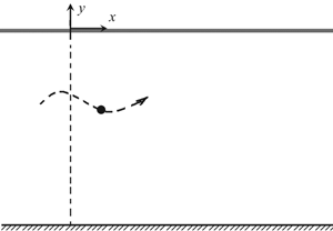
2. Motion of a point source in a water. Problem statement and the general solution
Consider a fixed rectangular coordinate system  $Oxy$, where the
  $x$-axis coincides with the unperturbed upper boundary of the water, and the positive direction of the
  $y$-axis is upward. The water of total depth
  $H$ is assumed to be incompressible, inviscid and homogeneous, and its motion is assumed to be potential. The upper boundary of the water is covered with a relatively thin layer of ice, which is considered as an elastic material of uniform density under a uniform stress. It is assumed that the water motion occurs in the result of the action of a point mass source of a variable intensity; the source turns on at time
  $t = 0$. The source position at
  $t \ge 0$ is determined by its trajectory
  $\boldsymbol {\xi } = (\xi (t), \eta (t))$ and the intensity
  $\mu (t)$, where
  $-H < \eta (t) < 0$ and
  $\mu (t) = 0$ for
  $t < 0$.
As we assumed above that the water motion is irrotational, it can be described by the velocity potential  $\varPhi (x, y, t)$, so that the fluid velocity vector
  ${\boldsymbol {V}} = \boldsymbol {\nabla } \varPhi$, where the potential satisfies the Poisson equation
 \begin{equation} {\rm \Delta} \varPhi = \mu (t) \delta (\boldsymbol{x} - {\boldsymbol\xi}(t)) \quad (|x| < \infty, \ -H \le y \le 0). \end{equation}
Here,  ${\rm \Delta}$ denotes the two-dimensional Laplace operator in the
  $(x, y)$-plane,
  $\boldsymbol {x}=(x, y)$, and
  $\delta$ is the Dirac delta function.
Then we assume that the lower boundary of the ice plate is always in contact with the water. Denoting by  $w(x, t)$ the vertical displacements of the ice plate from the unperturbed position, we present the kinematic and dynamic boundary conditions at
  $y = 0$, respectively (see, for example, Squire et al. Reference Squire, Hosking, Kerr and Langhorne1996)
 \begin{gather} \frac{\partial w}{\partial t} - \frac{\partial \varPhi}{\partial y} = 0, \end{gather}
 \begin{gather}D\frac{\partial^4 w}{\partial x^4} + Q\frac{\partial^2 w}{\partial x^2} + M\frac{\partial^2 w}{\partial t^2} = -\left(\rho\frac{\partial \varPhi}{\partial t} + \rho gw \right), \end{gather}
where  $D = Eh_1^3/[12(1 - \nu ^2)]$,
  $M = \rho _1h_1$,
  $E$ is the Young's modulus of the elastic plate,
  $Q$ is the longitudinal stress (
 $Q > 0$ corresponds to compression, and
  $Q < 0$ to stretching), other parameters are
  $\nu$ the Poisson ratio,
  $\rho _1$ the ice density and
  $h_1$ the thickness of the ice plate;
  $\rho$ is the density of water,
  $g$ is the acceleration due to gravity. The first term in (2.3) describes the elastic property of the ice plate; the second term represents a horizontal stress or strain of the plate; the third term describes the inertial property of ice plate; the two terms on the right-hand side represent a pressure on the surface for small-amplitude potential oscillations of a fluid. The bottom is assumed non-permeable, so that at
  $y = -H$ we have
 \begin{equation} \frac{\partial \varPhi}{\partial y} = 0. \end{equation}
 It is assumed that far from the source the water is calm and the velocity field is identically zero for all  $t > 0$
 \begin{equation} \lim_{r \to \infty} \boldsymbol{\nabla} \varPhi = 0,\quad \text{where } r = |x - \xi (t) |. \end{equation}
 The initial conditions at  $y = 0$ and all
  $x$ are
 \begin{equation} \varPhi = w = \partial w / \partial t = 0, \quad t = 0. \end{equation}
To solve the initial-boundary value problem (2.1)–(2.6) we use the Laplace and Fourier transforms
 \begin{equation} \hat{\varPhi}(k,y,s)=\int_0^\infty \textrm{e}^{-st}\int_{-\infty}^{+\infty} \varPhi(x,y,t)\,\textrm{e}^{-\mathrm{i}kx}\,\textrm{d}x\,\textrm{d}t \end{equation}
with  $\mbox {Re}(s) > 0$ and real
  $k$. In the result, we obtain the ordinary differential equation for
  $\hat {\varPhi } (k, y, s)$ (the prime stands for differentiation with respect to
  $y$)
$y$)
 \begin{equation} \hat{\varPhi}''-k^2\hat{\varPhi}=\int_0^\infty\mu(t)\exp({-st-\mathrm{i}k\xi(t)}) \delta(y-\eta(t))\,\textrm{d}t \end{equation}
with the boundary conditions
 \begin{equation} [\varUpsilon(k)+Ms^2]\hat{\varPhi}'+\rho s^2\hat{\varPhi}=0 \ (y=0), \quad \hat{\varPhi}'=0 \ (y=-H), \end{equation}
where  $\varUpsilon (k) = Dk^4 - Qk^2 + \rho g$.
Our main interest in this problem is the determination of the vertical displacements of the ice plate from the unperturbed plane position. The Laplace and Fourier transforms for the function  $w(x, t)$ can be found from the formula
  $\hat {w}(k, s) = \hat {\varPhi }'(k, 0, s)/s$ which follows from (2.2). Solving (2.8) with the boundary conditions (2.9a,b) and substituting to this formula, we find
 \begin{equation} \hat{w}=\frac{\rho s}{B(k)[s^2+\omega^2(k)]\cosh{kH}}\int_0^\infty\mu(t)\exp({-st-\mathrm{i}k\xi(t)}) \cosh{[k(H+\eta(t))]}\,\textrm{d}t, \end{equation}
where  $B(k) = \rho + Mk\tanh {kH}$ and the dispersion relation for the linear wave perturbations is
 \begin{equation} \omega(k) = \sqrt{\frac{Dk^4 - Qk^2 + \rho g}{\rho + Mk\tanh{kH}}k\tanh{kH}}. \end{equation}
 The ice plate deformation in the real  $(x, t)$-space can be formally obtained by means of inverse Fourier and Laplace transforms
 \begin{equation} w(x,t)=\frac{\rho}{2{\rm \pi}}\int_{-\infty}^\infty\frac{G(k,x,t)\,\textrm{d}k}{B(k)\cosh{kH}}, \end{equation}
where
 \begin{gather} G(k,x,t) = \int_0^\infty\mu(\tau)\exp({\mathrm{i}k(x-\xi(\tau))})\cosh{[k(H+\eta(\tau))]}Z(k,t,\tau)\,\textrm{d}t, \end{gather}
 \begin{gather}Z(k,t,\tau) = \frac{1}{2\mathrm{i}{\rm \pi}}\int_{\lambda-\mathrm{i}\infty}^{\lambda+\mathrm{i} \infty}\frac{s\,\textrm{e}^{s(t-\tau)}}{s^2+\omega^2(k)}\,\textrm{d}s. \end{gather}
 The value of  $\lambda$ should be chosen such that the integration path in (2.14) lies to the right of all singular points of the integrand, which are the roots of the equation
  $s^2 + \omega ^2 (k) = 0$. It is clear that this equation has only two purely imaginary roots
  $s = \pm \mathrm {i} \omega (k)$. The function
  $Z$ is non-zero only for
  $t > \tau$ and is equal to
 \begin{equation} Z = \cos{[\omega(k)(t-\tau)]}, \quad (t > \tau). \end{equation}
 Finally, the solution for the function  $w(x,t)$ takes the form
 \begin{align} w(x,t)&=\frac{\rho}{\rm \pi}\int_0^\infty\frac{\textrm{d}k}{B(k)\cosh{kH}}\nonumber\\ &\quad \times{} \int_0^t\mu(\tau) \cos{[k(x-\xi(\tau))]}\cos{[\omega(k)(t-\tau)]}\cosh{[k(H+\eta(\tau))]}\,\textrm{d}\tau. \end{align}
3. The motion of a dipole
In this paper we consider the linearized problem, therefore the solution to the set of equations (2.1)–(2.6) can be presented as a linear combination of mass sources and sinks. The simplest example of a moving body that can be modelled by point sources in the two-dimensional case is a horizontal circular cylinder moving perpendicular to its axis. The motion of such a cylinder is simulated by a dipole with the moment  ${\boldsymbol {M}}(t) = M_0{\boldsymbol {U}}(t)$, where
  $M_0 = 2{\rm \pi} R^2$,
  ${\boldsymbol {U}} = (U_1, U_2) = \textrm {d}{\boldsymbol \xi }(t)/\textrm {d}t$,
  $\boldsymbol {x} = {\boldsymbol {\xi }}(t)$ is the trajectory of the cylinder centre, and
  $R$ is its radius.
Solution for vertical displacement of the elastic ice plate caused by the motion of a dipole, has the form
 \begin{align} w(x,t) &= \frac{\rho M_0}{\rm \pi}\int_0^\infty\frac{k\,\textrm{d}k}{B(k)\cosh{kH}} \int_0^t\left\{U_1(\tau)\sin{[k(x-\xi(\tau))]}\cosh{[k(H+\eta(\tau))]} \right.\nonumber\\ &\quad \left.+ U_2(\tau)\cos{[k(x-\xi(\tau))]}\sinh{[k(H+\eta(\tau))]}\right\}\cos{[\omega(k)(t-\tau)]}\,\textrm{d}\tau. \end{align}
 Further, we restrict ourselves to considering the motion of the dipole moving only in the horizontal direction at a fixed depth  $h$ and set
  $U_2(t)=0$,
  $\eta (t) = -h$.
3.1. Horizontally translating dipole with constant speed
When a dipole instantly accelerates from zero to a constant speed  $U_0$, its trajectory is determined by the formula
 \begin{equation} \xi(t)=U_0 t, \quad U_1(t)=U_0. \end{equation}
 Then, in the moving coordinate system  $X = U_0t - x$ associated with the stationary dipole and oriented such that the flow runs on it from the left, solution (3.1) takes the form
 \begin{equation} w(X,t) = \frac{\rho M_0U_0}{\rm \pi}\int_0^\infty\frac{k\cosh{[k(H-h)]}}{B(k)\cosh{kH}}\int_0^t \sin{[k(U_0p - X)]}\cos{[\omega(k)p]}\,\textrm{d}p\,\textrm{d}k. \end{equation}
After evaluation of the inner integral, we obtain
 \begin{equation} w(X,t) = \frac{\rho M_0U_0}{2{\rm \pi}}\int_0^\infty\frac{k\cosh{[k(H-h)]}}{B(k)\cosh{kH}} \left[I_c(k)\cos{kX} - I_s(k)\sin{kX}\right] \textrm{d}k, \end{equation}
where
 \begin{gather} I_c(k) = \frac{1-\cos{[(U_0k+\omega(k))t]}}{U_0k + \omega(k)} + \frac{1-\cos{[(U_0k - \omega(k))t]}}{U_0k - \omega(k)}, \end{gather}
 \begin{gather}I_s(k) = \frac{\sin{[(U_0k + \omega(k))t]}}{U_0k + \omega(k)} + \frac{\sin{[(U_0k - \omega(k))t]}}{U_0k - \omega(k)}. \end{gather}
Next, we consider a horizontally oscillating dipole with zero mean velocity.
3.2. Horizontally oscillating dipole with zero mean velocity
When a dipole oscillates horizontally with constant amplitude  $\gamma$ and frequency
  $\varOmega$, its trajectory has the form
 \begin{equation} \xi(t) = \gamma \sin{\varOmega t}, \quad U_1(t) = \gamma \varOmega\cos{\varOmega t}. \end{equation}
Then, the vertical oscillations of elastic ice plate are
 \begin{align} w(x,t) &= \frac{\rho\gamma\varOmega M_0}{\rm \pi}\int_0^\infty\frac{k\cosh{[k(H-h)]}}{B(k)\cosh{kH}}\nonumber\\ &\quad \times \int_0^t\cos{\varOmega\tau}\sin{[k(x-\gamma\sin(\varOmega \tau))]}\cos{[\omega(k)(t-\tau)]}\,\textrm{d}\tau\,\textrm{d}k. \end{align}
 For small-amplitude oscillations when  $\gamma \to 0$, this formula can be simplified and presented as
 \begin{equation} w(x,t) = \gamma[w_c(x,t)\cos{\varOmega t} + w_s(x,t)\sin{\varOmega t}], \end{equation}
where
 \begin{gather} w_{c,s}(x,t) = \frac{\rho\varOmega M_0}{2{\rm \pi}}\int_0^\infty\frac{k\sin{kx}\cosh{[k(H-h)]}}{B(k)\cosh{kH}}P_{c,s}(k,t)\,\textrm{d}k, \end{gather}
 \begin{gather}P_c(k,t) = \frac{\sin{[(\varOmega + \omega(k))t]}}{\varOmega + \omega(k)} + \frac{\sin{[(\varOmega-\omega(k))t]}}{\varOmega - \omega(k)}, \end{gather}
 \begin{gather}P_s(k,t) = \frac{1-\cos{[(\varOmega+\omega(k))t]}}{\varOmega + \omega(k)} + \frac{1-\cos{[(\varOmega-\omega(k))t]}}{\varOmega - \omega(k)}. \end{gather}
Now we can combine the two types of dipole motion described above using the principle of superposition for a linear system.
3.3. Horizontally moving and oscillating dipole
Assume now that a dipole moves horizontally and periodically oscillates in the direction of motion. Its trajectory is described by the formula
 \begin{equation} \xi(t) = U_0 t + \gamma \sin{\varOmega t}, \quad U_1(t) = U_0 + \gamma\varOmega\cos{\varOmega t}. \end{equation}
 In the moving coordinate system  $X = U_0t - x$, the solution (3.1) has the form
 \begin{align} w(X,t)&=\frac{\rho M_0}{\rm \pi}\int_0^\infty\frac{k\cosh{[k(H-h)]}}{B(k)\cosh{kH}}\int_0^t(U_0 + \gamma\varOmega\cos{\varOmega \tau}) \nonumber\\ &\quad \times \sin{\{k[U_0(t - \tau) - X - \gamma\sin{\varOmega \tau}]\}}\cos{[\omega(k)(t - \tau)]}\,\textrm{d}\tau\,\textrm{d}k. \end{align}
For small-amplitude oscillations of the dipole this formula can be further linearized with respect to  $\gamma$, as above, and presented in the form
 \begin{equation} w(X,t) = w_0(X,t) + \gamma\left[W_c(X,t)\cos{\varOmega t} + W_s(X,t)\sin{\varOmega t}\right], \end{equation}
where function  $w_0(X,t)$ is the same as in (3.4), and functions
  $W_c(X,t)$ and
  $W_s(X,t)$ are given by the formulae
 \begin{align} W_c(X,t) &= \frac{\rho M_0\varOmega}{\rm \pi}\int_0^\infty\frac{k\cosh{[k(H-h)]}}{B(k)\cosh{kH}} \nonumber\\ &\quad \times \int_0^t\cos{\varOmega p}\sin{[k(U_0p-X)]}\cos{[\omega(k) p]}\,\textrm{d}p\,\textrm{d}k,\end{align}
 \begin{align} W_s(X,t) &= \frac{\rho M_0\varOmega}{\rm \pi}\int_0^\infty\frac{k\cosh{[k(H-h)]}}{B(k)\cosh{kH}} \nonumber\\ &\quad \times \int_0^t \sin{\varOmega p}\sin{[k(U_0p-X)]}\cos{[\omega(k) p]}\,\textrm{d}p\,\textrm{d}k. \end{align}
 To study the behaviour of functions  $W_c$ and
  $W_s$ in the far-field zone when
  $|X|,t \to \infty$ we will use the method of stationary phase to estimate asymptotically the double integral (3.16) and (3.17). The phase functions in these integrals have the following forms:
 \begin{gather} \varPsi_{1,2}(k,p) = k(U_0p - X)\pm p[\varOmega + \omega(k)], \end{gather}
 \begin{gather}\varPsi_{3,4}(k,p) = k(U_0p - X)\pm p[\varOmega - \omega(k)]. \end{gather}
The stationary points are solutions of the following set of simultaneous equations:
 \begin{gather} \frac{\partial\varPsi_i}{\partial k} = 0, \quad \rightarrow \quad \frac{\textrm{d}\omega}{\textrm{d}k} = \pm\left(U_0 - \frac{X}{p}\right), \end{gather}
 \begin{gather}\frac{\partial\varPsi_i}{\partial p} = 0, \quad \rightarrow \quad \frac{\omega}{k} = \pm\frac{\varOmega}{k} \pm U_0. \end{gather}
We will use these equations in the following sections, and now we will present the analysis of the dispersion relation (2.11).
4. Analysis of the dispersion relation
The behaviour of flexural–gravity waves (FGW) in a fluid covered by a floating elastic plate is determined by the dispersion relation, which establishes a relationship between the wavenumber  $k$ and frequency
  $\omega$ as per (2.11). The phase and group velocities can be readily found from the dispersion relation
 \begin{gather} c_p \equiv \frac{\omega}{k} = \sqrt{\frac{(Dk^4-Qk^2+\rho g)\tanh{kH}}{k(\rho+kM\tanh{kH})}}, \end{gather}
 \begin{gather}c_g \equiv \frac{\textrm{d}\omega}{\textrm{d}k} = \frac{Z(k)}{2\omega(k)(\rho+kM\tanh{kH})^2}, \end{gather}
where
 \begin{align} Z(k) &= 2k^3M(2Dk^2-Q)\tanh^2{kH} + \rho Hk(Dk^4-Qk^2+\rho g)(1 - \tanh^2{kH}) \nonumber\\ &\quad + \rho(5Dk^4-3Qk^2+\rho g)\tanh{kH}. \end{align}
 As is well known, the dispersion relation (2.11) imposes a restriction on the maximal value of a compression force. The stability of oscillations of a floating ice plate is guaranteed by the condition  $Q < Q_* \equiv 2\sqrt {g\rho D}$, whereas at
  $Q > Q_*$ the ice plate shatters (see, for example, Kheisin Reference Kheisin1967; Bukatov Reference Bukatov2017). There is one more critical value of the parameter
  $Q$ such that for
  $Q < Q_0 < Q_*$ the group velocity of FGW is positive for all wavenumbers
  $k \ge 0$. Such a case when
  $c_g > 0$ will be called normal dispersion in contrast to the case of anomalous dispersion for
  $Q_0 < Q < Q_*$, which is characterized by the presence of a wavenumber interval within which the group velocity is negative (see below). Both these critical values
  $Q_*$ and
  $Q_0$, as well as the corresponding wavenumbers
  $k_*$ and
  $k_0$, can be determined from the joint solution of two simultaneous equations
  $c_g(k) = 0$ and
  $\textrm {d}c_g/\textrm {d}k = 0$.
In the case of infinitely deep water when  $kH \to \infty$ the formulae (2.11) and (4.1)–(4.3) simplify and become
 \begin{gather} \omega(k) = \sqrt{\frac{k(Dk^4-Qk^2+\rho g)}{\rho+kM}}, \end{gather}
 \begin{gather}c_p = \sqrt{\frac{Dk^4-Qk^2+\rho g}{k(\rho+kM)}}, \end{gather}
 \begin{gather}c_g = \frac{2k^3M(2Dk^2-Q)+\rho(5Dk^4-3Qk^2+\rho g)}{2\omega(k)(\rho+kM)^2}, \end{gather}
 \begin{gather}\frac{\textrm{d}c_g}{\textrm{d}k} = \frac{3\rho^2 k^4 Q^2 - 2k^2AQ + B}{4\omega^3(k)(\rho+kM)^4}, \end{gather}
where
 \begin{align} A = 6DM^2k^6 + 14DM\rho k^5 + 11D\rho^2k^4 + 2M^2\rho gk^2 + 2M\rho^2gk + 3\rho^3 g, \end{align}
 \begin{align} B &= 8D^2M^2k^{10} + 20D^2M\rho k^9 + 15D^2\rho^2k^8 + 24DM^2\rho gk^6 + 48DM\rho^2gk^5 \nonumber\\ &\quad + 30D\rho^3g k^4 - 4M\rho^3g^2k - \rho^4 g^2. \end{align}
 Equating the group velocity (4.6) and its derivative (4.7) to zero and eliminating  $Q$, we find the equation to determine the critical values for
  $k$
$k$
 \begin{equation} \left(Dk^4 - \rho g\right)\left(8DMk^5 + 15\rho Dk^4 - 3g\rho^2\right) = 0. \end{equation}
 From the expression in the first bracket we find  $k_* = \sqrt [4]{\rho g/D}$, and from the expression in the second bracket we obtain a fifth degree polynomial the positive root of which defines the second critical point
  $k_0$
$k_0$
 \begin{equation} 8DMk_0^5 + 15\rho Dk_0^4 - 3g\rho^2 = 0. \end{equation}
Then we find
 \begin{equation} Q_* = 2\sqrt{\rho gD}, \quad Q_0 = \frac{10Dk_0^2}{3}. \end{equation}
If  $M$ is negligibly small, then
  $k_0 = k_*/\sqrt [4]{5} \approx 0.67k_*$, and
  $Q_0 = 2\sqrt {5}Dk_*^2/3$.
Figure 1 illustrates a fragment of the polynomial (4.11) in the dimensionless form  $P(\kappa , K) = 8K\kappa ^5 + 15\kappa ^4 - 3$, where
  $\kappa = k/k_*$, and
  $K = \sqrt [4]{\rho g/D}$.

Figure 1. Fragment of the polynomial  $P(\kappa , K)$ for three values of
  $K$. Line 1 pertains to
  $K = 1$, line 2 to
  $K = 10$, and line 3 to
  $K = 10^{-3}$. Dashed vertical line restricts the admissible values of
  $\kappa < 1$; small vertical arrow indicates the limiting value of
  $\kappa _0 \equiv k_0/k_* = 1/\sqrt [4]{5} \approx 0.67$ when
  $K \to 0$.
4.1. Numerical solution of the dispersion relation
To investigate the dispersion relation quantitatively, we set the following values for the parameters:
 \begin{equation} \left.\begin{gathered}
\rho_1 = 922.5\ \mbox{kg} \ \textrm{m}^{-3},\quad h_1 =
1 \ \mbox{m}, \quad E = 5\times 10^9\ \mbox{Pa}, \ \nu =
0.3,\\ \rho = 1025\ \mbox{kg} \ \textrm{m}^{-3}, \quad h =
10 \ \mbox{m}, \quad R = 5\ \mbox{m}, \quad g = 9.81 \
\mbox{m} \ \textrm{s}^{-2}. \end{gathered}\right\}
\end{equation}
\begin{equation} \left.\begin{gathered}
\rho_1 = 922.5\ \mbox{kg} \ \textrm{m}^{-3},\quad h_1 =
1 \ \mbox{m}, \quad E = 5\times 10^9\ \mbox{Pa}, \ \nu =
0.3,\\ \rho = 1025\ \mbox{kg} \ \textrm{m}^{-3}, \quad h =
10 \ \mbox{m}, \quad R = 5\ \mbox{m}, \quad g = 9.81 \
\mbox{m} \ \textrm{s}^{-2}. \end{gathered}\right\}
\end{equation}
We remind the reader that, here,  $R$ is the radius of a cylinder moving at the depth
  $h$ (see § 3). Three values for the total depth were chosen,
  $H=100$ m,
  $H=40$ m and infinite depth,
  $(H = \infty )$.
Figure 2 shows the dispersion relation (2.11) in dimensionless form for the parameters indicated above (4.13) and  $H=40$ m. The dispersion curves were plotted for five values of the parameter
  $\tilde {Q} \equiv Q/\sqrt {g\rho D} = 0, 1.2, 1.8, 1.95, 2$. As one can see, the dispersion is normal (the corresponding curves are monotonically increasing) for the first two values of
  $\tilde {Q}$ and anomalous for the other three values.

Figure 2. Dispersion relations for the FGW for the different values of the compression parameter  $Q$.
$Q$.
In table 1 we present the values of  $k_0R$ and
  $\tilde {Q}_0 \equiv Q_0/\sqrt {g \rho D}$ for the parameters indicated above (4.13) for three different depths.
Table 1. Values of  $k_0R$ and
  $\tilde {Q}_0$ for the typical parameters indicated in (4.13) for three different depths.

The influence of water depth is noticeable only for relatively small wavenumbers. This is illustrated by figure 3, where the dispersion relation is shown in the range  $0 \le kR \le 0.3$ for three values of the water depth and two values of the parameter
  $\tilde {Q}$ characterizing the compression effect.

Figure 3. Dispersion relation of FGW for three values of water depth  $H$ and two values of the compression parameter
  $\tilde {Q}$. (a)
  $\tilde {Q} = 1.2$, (b)
  $\tilde {Q} = 2$. In both panels line 1 pertains to
  $H = 40$ m, line 2 pertains to
  $H = 100$ m and line 3 pertains to infinite depth
  $H = \infty$ m.
In figures 4 and 5 we present the dependences of phase and group speeds at  $H = 40$ m (solid lines) and
  $H = \infty$ (dashed-dotted lines) for two values of the compression parameter
  $\tilde {Q} = 1.2$ and
  $\tilde {Q} = 1.95$, respectively. For a finite fluid depth in the long-wave limit we obtain
  $c_p(0) = c_g(0) = \sqrt {gH}$, whereas for infinitely deep water when
  $k \to 0$ we have
  $c_p = 2c_g \approx \sqrt {g/k}$. When
  $k \to \infty$,
  $c_g = 2c_p \approx 2k\sqrt {D/M}$ regardless of fluid depth.

Figure 4. Phase  $c_p$ and group
  $c_g$ speeds of FGW for
  $\tilde {Q} = 1.2$. Solid lines pertain to
  $H = 40$ m, and dashed lines to
  $H = \infty$ m.

Figure 5. The same as figure 4, but for  $\tilde {Q} = 1.95$.
From these figures we see again that the effect of water depth is noticeable only at relatively small wavenumbers  $0 \le kR \le 0.3$. The behaviours of both phase and group velocities are non-monotonic for FGW, since both speeds have local minima. As can be seen from the graphs for the group velocity with the abnormal dispersion, figure 5, there are two values of the wavenumber
  $k_1$ and
  $k_2$ (
 $k_1 < k_2$) where the group velocity turns to zero. The dispersion curve has local extrema at these points, and
  $\omega (k_1) > \omega (k_2)$. The dependencies
  $k_1$,
  $k_2$ and
  $\omega (k_1)$,
  $\omega (k_2)$ on the parameter
  $\tilde {Q}$ are shown in figures 6 and 7, respectively, for two different fluid depths,
  $H = 40$ m (solid lines) and
  $H = \infty$ m (dashed lines).

Figure 6. Dependences of  $k_1R$ and
  $k_2R$ on the parameter
  $\tilde {Q}$ for
  $H = 40$ m (solid line) and
  $H = \infty$ m (dashed line).

Figure 7. Dependences of  $\omega _1\sqrt {R/g}$ and
  $\omega _2\sqrt {R/g}$ on the parameter
  $\tilde {Q}$ for
  $H = 40$ m (solid line) and
  $H = \infty$ m (dashed line).
The  $\times$-symbol in figure 6 marks the value of
  $\tilde {Q}_0$ for a particular water depth, so that we have the dependence of
  $k_1R(\tilde {Q})$ to the left and
  $k_2R(\tilde {Q})$ to the right of this point.
5. Analysis of wave perturbations with a different character of dipole motion
5.1. Flexural–gravity waves generated by the uniform horizontal motion of a dipole
In this particular case, when  $\varOmega = 0$, we see from the expressions (3.18), (3.19) that the only solution for the stationary points is possible when
 \begin{equation} c_p(k_c) = U_0, \quad p_c = \frac{X}{U_0 - c_g(k_c)}. \end{equation}
The first equation in (5.1a,b) has
(i) no roots for
 $U_0 < (c_p)_{min}$, where $(c_p)_{min}$ is the minimum phase velocity of FGW;
(ii) two roots
$k_{1,2} \ (k_1 < k_2)$ for $(c_p)_{min} < U_0 < \sqrt {gH}$; and(iii) only one root
$k_{2}$ for $U_0 > \sqrt {gH}$.


Therefore, for  $U_0 < (c_p)_{min}$, the wave motion far from the dipole is absent. For
  $(c_p)_{min} < U_0 < \sqrt {gH}$ a wave with the wavenumber
  $k_{1}$ exists only for
  $X > 0$, and a wave with the wavenumber
  $k_{2}$ only if
  $X < 0$. This means that the wave motion exists both in front and behind the moving dipole; moreover, the length of the generated wave for
  $X > 0$ is greater than for
  $X < 0$. For
  $U_0 > \sqrt {gH}$, a wave motion exists only in front of a moving dipole at
  $X < 0$. From the second equation (5.1a,b) it follows that the wave fronts (i.e. the boundaries dividing the regions of water perturbed by the waves from the regions where water is unperturbed) move relative to the source to the right and to the left with speeds
  $U_0 - c_g(k_{1,2})$, respectively. In the motionless coordinate system the wave fronts move in the corresponding directions with the group velocities of generated waves.
5.2. Flexural–gravity waves generated by a horizontally oscillating dipole
Consider now a horizontally oscillating dipole and the flexural–gravity waves generated by it. In this case, in expressions (3.18), (3.19) we have  $U_0 = 0$, and the asymptotic analysis shows that the wave pattern has a certain symmetry relative to the origin and can contain from one to three wave harmonics. Stationary points now have only the functions
  $\varPsi _ {3,4}$ in (3.19), and those equations reduce to
 \begin{equation} \varPsi_{3}(k,p) = kx + p[\varOmega-\omega(k)], \quad \varPsi_{4}(k,p) = kx-p[\varOmega-\omega(k)]. \end{equation}
 In the case of normal dispersion, i.e. for  $Q < Q_0$, each function
  $\varPsi _3$ and
  $\varPsi _4$ in (5.2a,b) has a unique stationary point with the same wavenumber
  $k_1$, which is defined by the expression
 \begin{equation} \omega(k_1) = \varOmega. \end{equation}
The value of  $p_1$ in the immovable coordinate system equals to
  $\pm x/c_g (k_1)$, respectively. Therefore, the wave defined by the stationary point of the function
  $\varPsi _3$ exists only for
  $x > 0$, and the wave determined by the stationary point of the functions
  $\varPsi _4$ exists only for
  $x < 0$. The speeds of front propagations of these waves are equal to
  $\pm c_g(k_1)$, respectively.
In the case of anomalous dispersion when  $Q_0 < Q <Q_*$, as shown above, there are values of
  $k_1$ and
  $k_2$
$k_2$  $(k_1 < k_2)$ in which the group velocity of the FGW vanishes, and the group velocity is negative in the interval
  $k_1 < k < k_2$. In the frequency range
  $\omega (k_2) < \varOmega < \omega (k_1)$, the functions
  $\varPsi _{3,4}$ in (5.2a,b) have three stationary points, which we denote
  $k^{(1)}$,
  $k^{(2)}$ and
  $k^{(3)}$
  $(k^{(1)} < k^{(2)} < k^{(3)})$. The values of
  $k^{(\,j)}$ with
  $(\,j = 1, 2, 3)$ satisfy (5.3) with the replacement of
  $k_1$ by
  $k^{(\,j)}$. In this case, the waves which are determined by the stationary points
  $k^{(1)}$ and
  $k^{(3)}$ of the function
  $\varPsi _3$ exist only at
  $x > 0$, whereas a wave determined by
  $k^{(2)}$ exists only at
  $x < 0$. The opposite situation occurs for waves determined by the stationary points of the function
  $\varPsi _4$. As the result, we have a symmetrical wave pattern with respect to
  $x$. Far from the dipole there is a system of three waves whose front propagation velocities are
  $\pm c_g(k^{(\,j)})$
  $(\,j = 1, 2, 3)$.
5.3. Flexural–gravity waves generated by the superposition of the translating and oscillating dipole motion
In this subsection we restrict ourselves to the consideration of an infinitely deep fluid, because in this case, the definition of stationary points of the functions  $\varPsi _i(k, p)$
  $(i = 1, 2, \ldots , 4)$ in (3.18), (3.19) reduces to the determination of the roots of polynomials, whereas in the case of a fluid of finite depth it is necessary to solve transcendental equations.
It is convenient to transform the dimensionless variables in which the radius of a cylinder  $R$ plays a role of the length scale, and the parameter
  $\sqrt {R/g}$ plays a role of the time scale. Then the main dimensionless parameters are as follows:
 \begin{equation} \bar{D} = \frac{D}{g\rho R^4}, \quad \bar{M} = \frac{M}{\rho R}, \quad \bar{Q} = \frac{Q}{g\rho R^2}, \quad F=\frac{U_0}{\sqrt{gR}}, \quad \sigma = \varOmega\sqrt{\frac{R}{g}}. \end{equation}
The dispersion relation (4.4) in the dimensionless variables has a form
 \begin{equation} \bar{\omega}(\bar{k}) = \sqrt{\frac{\bar{k}(\bar{D}\bar{k}^4 - \bar{Q}\bar{k}^2 + 1)}{1 + \bar{k}\bar{M}}}, \end{equation}
where  $\bar {\omega } = \omega \sqrt {R/g}$,
  $\bar {k} = kR$.
Function  $\varPsi _1$ in (3.18) does not have stationary points, because the determining equation
 \begin{equation} \bar{k}F + \sigma + \bar{\omega}(\bar{k}) = 0 \end{equation}
does not have positive real roots.
Function  $\varPsi _2$ in (3.18) also does not have stationary points if
  $F < V_1(\sigma )\equiv \bar {c}_g(k_1^*)$, where
  $\bar {c}_g = c_g/\sqrt {gR}$ and the wavenumber
  $k_1^*$ is the root of equation
 \begin{equation} \bar{k}\bar{c}_g(\bar{k}) - \bar{\omega}(\bar{k}) = \sigma. \end{equation}
 If, however,  $F > V_1(\sigma )$, then function
  $\varPsi _2$ in (3.18) has two stationary points and the determining equation
 \begin{equation} \bar{k}F - \sigma - \bar{\omega}(\bar{k}) = 0 \end{equation}
has two roots, which we denote as  $k_2^{(1)}$ and
  $k_2^{(2)}$
  $(k_2^{(1)}<k_2^{(2)})$. The values of
  $k_2^{(i)}$
  $(i = 1,2)$ can be found as the positive roots of the fifth-degree polynomial
 \begin{equation} \bar{k}^2[\bar{D}\bar{k}^3-\bar{k}(\bar{Q}+\bar{M}F^2)-F(F-2\sigma\bar{M})]+\bar{k}(1+2\sigma F-\sigma^2\bar{M})-\sigma^2=0, \end{equation}
satisfying (5.8).
It follows from the dispersion relation (5.5) that  $k_1^* \to k_p$ and
  $V_1 \to F_p$ when
  $\sigma \to 0$, where
  $k_p$ determines the dimensionless wavenumber that corresponds to the minimal dimensionless phase velocity of FGW,
  $F_p = U_p/\sqrt {gR}$, and
  $U_p\equiv (c_p)_{min}$. The equation which allows us to determine
  $k_p$ has the form
 \begin{equation} \bar{D}k_p^4(2\bar{M}k_p+3) - \bar{Q}k_p^2-2\bar{M}k_p-1 = 0. \end{equation}
 Function  $\varPsi _3$ in (3.19) has at most three stationary points. Equation
 \begin{equation} \bar{k}F+\sigma-\bar{\omega}(\bar{k})=0 \end{equation}
always has one positive root  $k_3^{(1)}$ and two additional roots
  $k_3^{(2)}$ and
  $k_3^{(3)}$ provided that
  $\sigma < \sigma ^* \equiv \bar {\omega }(k_g) - k_gF_g$ and
  $V_3 < F < V_2$. The value of
  $k_g$ is such that the dimensionless group velocity of FGW
  $\bar {c}_g$ has a minimum
  $F_g$ at
  $\bar k = k_g$; it can be calculated as the positive root of the tenth-degree polynomial which is obtained by equating to zero the numerator in (4.7) and in dimensionless variables has the form
 \begin{align} &\bar{D}\bar{k}^5[4\bar{D}\bar{M}(2\bar{M}\bar{k} + 5)\bar{k}^4+C_1\bar{k}^3-28\bar{Q}\bar{M}\bar{k}^2+C_2\bar{k}+48\bar{M}]\nonumber\\ &\quad + \bar{k}^4C_3-4\bar{Q}\bar{M}\bar{k}^3-6\bar{Q}\bar{k}^2-4\bar{M}\bar{k}-1 = 0, \end{align}
where  $C_1 = 3(5\bar {D}-4\bar {Q}\bar {M}^2)$,
  $C_2 = 2(12\bar {M}^2-11\bar {Q})$,
  $C_3 = 30\bar {D} + 3\bar {Q}^2 - 4 \bar {Q}\bar {M}^2$. The value of
  $F_g$ can be evaluated from the dimensionless form of equation (4.6).
Functions  $V_2(\sigma )$ and
  $V_3(\sigma )$ are determined as follows:
  $V_2 = \bar {c}_g(k_2^*)$ and
  $V_3 = \bar {c}_g(k_3^*)$, where
  $k_2^* < k_g < k_3^*$ are the roots of the equation
 \begin{equation} \bar{\omega}(\bar{k}) - \bar{k}\bar{c}_g(\bar{k}) = \sigma. \end{equation}
As follows from the dispersion relation (5.5),  $k_2^* \to 0$,
  $k_3^* \to k_p$ and
  $V_2 \to \infty$,
  $V_3 \to F_p$ when
  $\sigma \to 0$, but
  $\{k_2^*, k_3^*\} \to k_g$ and
  $\{V_2, V_3\} \to F_g$ when
  $\sigma \to \sigma ^*$. The values of
  $k_3^{(\,j)}$
  $(\,j=1, 2, 3)$ are the positive roots of the fifth-degree polynomial
 \begin{equation} \bar{k}^2[\bar{D}\bar{k}^3-\bar{k}(\bar{Q}+\bar{M}F^2) - F(F+2\sigma\bar{M})] + \bar{k}(1 - 2\sigma F - \sigma^2\bar{M}) - \sigma^2=0, \end{equation}
which satisfy (5.11).
Function  $\varPsi _4$ in (3.19) has at most three stationary points. Equation
 \begin{equation} \bar{k}F - \sigma + \bar{\omega}(\bar{k}) = 0 \end{equation}
always has one positive root  $k_4^{(1)}$ and two additional roots
  $k_4^{(2)}$ and
  $k_4^{(3)}$ provided that
  $Q_0 < Q < Q_*$. The values
  $k_4^{(i)}$
  $(i = 1,2,3)$ can be determined as the positive roots of (5.9) which satisfy (5.15).
The direction of wave propagation which is determined by the stationary points of functions  $\varPsi _2$ and
  $\varPsi _3$ depends on the sign of the expression
  $F - \bar {c}_g(k)$, and for the function
  $\varPsi _4$ it depends on the sign of the expression
  $F + \bar {c}_g(k)$. In these expressions, the wavenumbers k must be replaced by the stationary values of the corresponding functions. Waves with a positive value of expressions
  $F \pm \bar {c}_g(k)$ propagate downstream
  $(X > 0)$, whereas waves with a negative value propagate upstream
  $(X < 0)$.
Figure 8 shows the dependences of  $V_j$
$V_j$  $(\,j = 1, 2, 3)$ on the dimensionless frequency
  $\sigma$ for three different values of the compression parameter
  $\tilde {Q} = 1.2$ (a),
  $\tilde {Q} = 1.8$ (b) and
  $\tilde {Q} = 1.95$ (c). Curves
  $V_1$,
  $V_2$,
  $V_3$ divide the plane of parameters
  $(\sigma -F)$ into several domains. In the case of normal dispersion (
 $\tilde {Q} = 1.2$), the plane
  $(\sigma -F)$ is divided into four domains
  $G_n$
$G_n$  $(n = 1, \ldots , 4)$. The domain
  $G_1$ (marked by vertical hatching) is bounded on the right by curve
  $V_1$, and on the left by curve
  $V_2$. The domain
  $G_2$ (marked by the combination of horizontal and vertical hatching) is bounded on the right by curve
  $V_2$, below by curve
  $V_1$ and on the left by the vertical
  $F$-axis. The domain
  $G_3$ (marked by horizontal hatching) is bounded on the right by curve
  $V_2$, on the left by curve
  $V_3$ and above by curve
  $V_1$. The remaining part of the plane
  $(\sigma -F)$ (not shaded domain) is denoted by
  $G_4$.

Figure 8. Dependences  $V_j$
$V_j$  $(\,j = 1, 2, 3)$ on the dimensionless frequency
  $\sigma$ for three values of the compression parameter
  $\tilde {Q} = 1.2$ (a),
  $\tilde {Q} = 1.8$ (b) and
  $\tilde {Q} = 1.95$ (c).
In the case of anomalous dispersion ( $\tilde {Q} =1.8, 1.95$), the domains
  $G_1$ and
  $G_2$ have the same boundaries as above, and the domain
  $G_3$ is now bounded by curves
  $V_1$,
  $V_2$,
  $V_3$ and
  $-V_3$. Meanwhile, two new domains appear:
  $G_5$ (shown by oblique hatching), bounded by curves
  $V_2$,
  $-V_2$,
  $-V_3$, as well as the domain
  $G_6$ (shown by combined horizontal and oblique hatching), bounded by the horizontal axes
  $\sigma$ and curves
  $V_2$,
  $-V_3$.
The vertical arrows on the horizontal axis show the values of  $\sigma ^*$, and the horizontal arrows on the vertical axis show the values of
  $|F_g|$. The common point of curves
  $V_1$ and
  $V_3$ on the vertical axis corresponds to the value of
  $F_p$.
Values of parameters  $k_p$,
  $F_p$,
  $k_g$,
  $F_g$ and
  $\sigma ^*$ for the used values of
  $\tilde {Q}$ are given in table 2.
Table 2. Values of parameters  $k_p$,
  $F_p$,
  $k_g$,
  $F_g$ and
  $\sigma ^*$ for the used values of
  $\tilde {Q}$.

In the case of normal dispersion (e.g. for  $\tilde {Q} = 1.2$):
(i) For the parameters
$\sigma$ and $F$ from the domain $G_1$, there are four stationary points $k_2^{(1)}$, $k_2^{(2)}$, $k_3^{(1)}$, $k_4^{(1)}$, two of which ($k_2^{(1)}$, and $k_4^{(1)}$) cause wave perturbations running downstream and the other two ($k_2^{(2)}$, $k_3^{(1)}$) running upstream.(ii) For the domain
$G_2$ there are six stationary points three of which ($k_2^{(1)}$, $k_3^{(2)}$, $k_4^{(1)}$) cause wave perturbations running downstream, and the other three ($k_2^{(2)}$, $k_3^{(1)}$, $k_3^{(3)}$) running upstream.(iii) For the domain
$G_3$ there are four stationary points two of which ($k_3^{(2)}$ and $k_4^{(1)}$) cause wave perturbations running downstream, and the other two ($k_3^{(1)}$ and $k_3^{(3)}$) running upstream.(iv) For the domain
$G_4$ there are only two stationary points, one of which $k_4^{(1)}$ causes wave perturbation propagating downstream, and another, $k_3^{(1)}$, running upstream.


In the case of anomalous dispersion, (e.g. for  $\tilde {Q} = 1.8$ or
  $\tilde {Q} = 1.95$):
(i) For the domain
$G_5$ there are four stationary points two of which ($k_4^{(1)}$ and $k_4^{(3)}$) cause wave perturbations running downstream, and the other two ($k_3^{(1)}$ and $k_4^{(2)}$) running upstream.(ii) For the domain
$G_6$ there are six stationary points, three of which ($k_3^{(2)}$, $k_4^{(1)}$ and $k_4^{(3)}$) cause wave perturbations running downstream, and the other three ($k_3^{(1)}$, $k_3^{(3)}$ and $k_4^{(2)}$) running upstream.


In the conclusion to this section we mention that the main properties of FGW were investigated by Bukatov (Reference Bukatov1980) by means of a different method (see also Bukatov Reference Bukatov2017). However, in our opinion the method described above is more visual. The three-dimensional case for an infinitely deep fluid with normal dispersion was described in detail by Sturova (Reference Sturova2013).
5.4. Analysis of vertical displacements of the ice plate
To get an idea of the real displacements of an ice plate caused by the motion of a dipole, we calculated the vertical displacements for the case of an infinitely deep water for the translational motion of the dipole using the integral representation (3.4), and for the superposition of the translational and oscillatory motions based on the integral representations (3.14), (3.15). The results can be characterized by the dimensionless parameter, the Froude number F =  $U_0/\sqrt {gR}$. Two typical values of the Froude number were chosen for the calculations, they are
  $F = 0.25$ and
  $F = 0.5$; the dimensionless frequency of oscillations were chosen as
  $\sigma = 0.2$ and 0.25; and the compression parameter was set to
  $\tilde {Q} = 0$ (no stress in the ice cover),
  $\tilde {Q} = 1.2$ and
  $\tilde {Q} = 1.95$.
The time variation of the vertical displacements of the ice plate in the case of translational motion of the dipole source with the Froude number  $F = 0.5$ is shown in the videos for the different values of the parameter
  $\tilde {Q}$ (see the links below).
(i)
$\tilde {Q} = 0$, https://eportfolio.usq.edu.au/view/view.php?t=4AoZqtbj07wsy8BWTrH1;(ii)
$\tilde {Q} \kern-0.2pt=\kern-0.4pt 1.2$, https://eportfolio.usq.edu.au/view/view.php?t=rDFPhJGxZNs8EKBHp2uo;(iii)
$\tilde {Q} = 1.95$, https://eportfolio.usq.edu.au/view/view.php?t=LAR34te01uXwV2fgkcvF.


Only in the case (iii) when  $\tilde {Q} = 1.95$ is the dipole motion supercritical. As shown in Savin & Savin (Reference Savin and Savin2012) and Il'ichev & Savin (Reference Il'ichev and Savin2017), in infinitely deep water after long-term motion of a dipole, a stationary wave
  $w_0(X)$ sets in the elastic plate
  $w_0(X, \infty )$ in the co-moving coordinate frame. In the subcritical regime of motion (
 $F < F_p$), a symmetrical-in-
 $X$ perturbation is formed in the elastic plate, which is a plate reaction to the dipole motion, and the minimum of the elevation is located directly above the dipole. In the dimensional variables the solution for the plate displacement
  $w_0(X)$ in the subcritical regime has the form
 \begin{equation} w_0(X) = -2\rho R^2 U_0^2\int_0^\infty \frac{k \,\textrm{e}^{-kh}\cos(kX)\,\textrm{d}k}{Dk^4 - \left(Q+MU_0^2\right)k^2 - \rho U_0^2k + g\rho}. \end{equation}
 In the supercritical regime ( $F> F_p$), the solution for the
  $w_0(X)$ has a more complex form
 \begin{equation} w_0(X) = 2\rho R^2 U_0^2\left[\left(\mu + 1\right)\chi(k_1)\sin(k_1X) + (\mu-1)\chi(k_2)\sin(k_2X) + K(X)\right], \end{equation}
where
 \begin{gather} K(X) = \int_0^\infty\frac{k\left[G(k)\cos(hk) + \rho U_0^2k\sin(hk)\right]}{G^2(k) + \rho^2U_0^4k^2}\,\textrm{e}^{-|X|k}\,\textrm{d}k,\end{gather}
 \begin{gather} G(k) = Dk^4 + \left(MU_0^2 + Q\right)k^2 + g\rho, \quad \chi(k_j) = \frac{{\rm \pi} k_j\,\textrm{e}^{-k_jh}}{P(k_j)}, \end{gather}
 \begin{gather} P(k) = 4Dk^3 - 2(Q + MU_0^2)k - \rho U_0^2. \end{gather}
Here,  $\mu = \mbox {sign}(X)$,
  $k_1$ and
  $k_2\ (k_1 < k_2)$ are roots of the equation
  $kU_0 = \omega (k)$. In the case of infinitely deep fluid this equation reduces to the polynomial
 \begin{equation} Dk^4 - \left(Q + MU_0^2\right)k^2 - \rho U_0^2k + g\rho = 0. \end{equation}
In the videos presented above the limiting solutions are shown in the very end by the dotted lines for the comparison with the transient solutions.
The behaviour of the elastic ice plate in superposition of the translational and oscillatory dipole motions is shown for  $F = 0.25$ and
  $\sigma = 0.25$ in figure 9. Panel (a) shows the plate oscillation for
  $\tilde {Q} = 1.2$ (this corresponds to the domain G4 in figure 8), and (b) shows the oscillation for
  $\tilde {Q} = 1.95$ (this corresponds to the domain G6).

Figure 9. Vertical displacements of elastic ice plate  $w(X, t)$ for superpositions of translational and oscillatory motions of the dipole with
  $F = 0.25$,
  $\sigma = 0.25$. Panel (a) pertains to
  $\tilde {Q} = 1.2$, and (b) to
  $\tilde {Q} = 1.95$. The time instants for each curve are indicated on the right of each panel. Calculations were performed on the basis of the linearized solution (3.15).
Figure 10 shows plate oscillations for  $F = 0.5$ and
  $\sigma = 0.2$. Panel (a) shows the plate oscillation for
  $\tilde {Q} = 1.2$ (this corresponds to the domain G4 in figure 8), and (b) shows the oscillation for
  $\tilde {Q} = 1.95$ (this corresponds to the domain G3).


The calculations were performed on the basis of the linearized solution (3.15) for  $\gamma /R = 0.5$ (the applicability of this solution presumes that
  $\varOmega R \ll 2U_0$). For comparison, in figure 10(a) we show by dark dots the complete solution (3.14) for the following parameters
  $F = 0.5$,
  $\sigma = 0.2$,
  $\tilde {Q} = 1.2$ and
  $\bar {t} = 3, \ 5$. It can be seen that, for the chosen amplitude of the dipole oscillation, the complete (3.14) and approximate (3.15) solutions practically coincide, whereas the calculation of the double integral in (3.14) requires significantly more computer resources and time-consuming calculation than the calculation of the single integral in (3.15) after analytic evaluation of the inner integrals in (3.16) and (3.17).
An increase in the compression coefficient  $\tilde {Q}$ leads to an increase of wave intensity both for the translational motion of the dipole and in the superposition of translational and oscillatory motions.
6. Steady-state oscillations of a circular cylinder under an ice cover
The modelling of a moving cylinder under an ice cover by the point dipole can look a bit doubtful because such modelling is correct, strictly speaking, only for a cylinder moving in an unbounded uniform fluid. The presence of the ice cover results in a correction to the shape of a body modelled by a dipole. The shape of the body can be determined, in principle, at each instant of time. However, the correction to the circular cylindrical shape caused by the presence of the ice sheet can be small if the cylinder moves relatively slowly and not too close to the ice sheet. It is intuitively expected that the generated small-amplitude waves in the linear approximation are not too sensitive to the shape of a moving body. In this section, we demonstrate quantitatively when these assumptions and expectations are correct by comparison of the characteristics of the wave motions onsetting at the flow around a solid circular cylinder and the dipole approximation of the cylinder. We present a solution for the steady oscillation of the ice plate generated by the moving circular cylinder, taking into account the boundary conditions on its surface. We compare wave amplitudes in the far-field zone and the damping coefficients derived by the multipole expansion method and within the dipole approximation. This aims to underpin the applicability of the dipole approximation if the aforementioned restrictions are fulfilled.
6.1. The problem statement
We assume that the wave motion is caused in the initially quiescent fluid by forced oscillations of a horizontal circular cylinder of a radius  $R$ with the frequency
  $\varOmega$ and amplitudes of horizontal and vertical displacements
  $\eta _{1,2}$ respectively. Assuming that the fluid motion is steady state, we write down the full velocity potential in the form
 \begin{equation} \varPhi(x,y,t) = \mbox{Re} \left[\textrm{i}\varOmega\sum_{j=1}^2\eta_j\varphi_j(x,y)\exp(\textrm{i}\varOmega t)\right]. \end{equation}
 Vertical displacements of the ice cover  $W(x,t)$ are determined from the relation
 \begin{equation} \frac{\partial W}{\partial t} = \left.\frac{\partial \varPhi}{\partial y}\right|_{y=0} \end{equation}
and by analogy with (6.1), it is convenient to write
 \begin{equation} W(x,t) = \mbox{Re}\left[\sum_{j=1}^2\eta_jw_j(x)\exp(\textrm{i}\varOmega t)\right]. \end{equation}
 In the bulk of water for the radiation potentials  $\varphi _j(x,y) \ (\,j = 1,2)$ the Laplace equation is satisfied
 \begin{equation} {\rm \Delta} \varphi_j=0 \quad (|x| < \infty,\ -\infty < y\leq 0). \end{equation}
At the upper boundary of the fluid,  $y = 0$, the kinematic and dynamic conditions are satisfied in accordance with conditions (2.2) and (2.3)
 \begin{equation} w_j(x)=\frac{\partial \varphi_j}{\partial y}, \quad \left(D\frac{\partial^4}{\partial x^4}+Q\frac{\partial^2}{\partial x^2}-M\varOmega^2 +\rho g\right)w_j-\rho \varOmega^2\varphi_j=0 \ (|x|<\infty). \end{equation}
On the circular contour of the cylinder  $\{S: \ x^2 + (y + h)^2 = R^2\}$, the non-leakage condition is assumed
 \begin{equation} \partial \varphi_j/\partial n=n_j \ (x,y \in S), \quad (\,j=1,2), \end{equation}
where  ${\boldsymbol {n}} = (n_1, n_2)$ is the internal normal to the contour
  $S$,
$S$,  $h$ is the distance of the cylinder centre from the upper boundary of the fluid
  $(h > R)$. For the infinitely deep fluid, the following condition secures the absence of fluid motion in the depth:
 \begin{equation} \nabla \varphi_j \to 0 \quad (y\to -\infty). \end{equation}
One more condition we use in the far-field zone requires the fulfilment of the radiation condition, that means that the generated waves are outgoing.
6.2. The multipole expansion method
To solve problem (6.4)–(6.7), the multipole expansion method is used (see, for example, Linton & McIver Reference Linton and McIver2001), which is the most effective method in studying bodies of a simple geometry: in the two-dimensional case – circles, in the three-dimensional case – spheres. Even and odd in  $x$ multipoles,
  $\cos (m\theta )/r^m$ and
  $\sin (m\theta )/r^m$, where
  $r = \sqrt {x^2 + (y + h)^2}$,
  $\theta = \arctan [x/(y + h)]$, are fundamental solutions of the Laplace equation singular at the point
  $x = 0$,
  $y = -h$.
The boundary condition (6.6) in terms of  $r,\theta$ has the form
 \begin{equation} \partial \varphi_1/\partial r = \sin{\theta}, \quad \partial \varphi_2/\partial r = \cos{\theta} \quad (r = R). \end{equation}
According to these boundary conditions, function  $\varphi _1(x,y)$ is odd, and function
  $\varphi _2(x,y)$ is even in the variable
  $x$.
$x$.
For the vertical oscillations of the cylinder solution  $\varphi _2(x,y)$ has the form
 \begin{equation} \varphi_2(x,y) = \sum_{m=1}^\infty p_m R^m\left[\frac{\cos(m\theta)}{r^m}+f_m(x,y)\right], \end{equation}
where
 \begin{gather} f_m(x,y) = \frac{1}{(m-1)!}\int_0^\infty k^{m-1}\cos(kx)A(k)\,\textrm{e}^{k(y+h)}\,\textrm{d}k, \end{gather}
 \begin{gather}A(k) = \frac{kP(k)+\rho \varOmega^2}{Z(k)}\,\textrm{e}^{-2kh}, \end{gather}
 \begin{gather}P(k) = Dk^4-Qk^2-M\varOmega^2+\rho g, \end{gather}
 \begin{gather}Z(k) = kP(k)-\rho\varOmega^2. \end{gather}
 The integrand in (6.10) has simple poles that are the roots of the equation  $Z(k) = 0$ which can be written as
  $\varOmega ^2 = \omega ^2(k)$, where
  $\omega (k)$ is the dispersion relation (4.4) for flexural–gravity waves in an infinitely deep fluid.
The function  $Z(k)$ is the fifth-degree polynomial which has only one real root
  $k = k_1 > 0$ if
  $Q < Q_0$, whereas for
  $Q_0 < Q < Q_*$ it has three real positive roots
  $k_n \ (n = 1,2,3)$ which we will arrange in the ascending order:
  $k_1 < k_2 < k_3$. The remaining roots of the polynomial are complex.
Taking into account the radiation condition in the far-field zone, we can present (6.10) in the form
 \begin{align} f_m(x,y) &= \frac{1}{(m-1)!}\left[P.V.\int_0^\infty k^{m-1}A(k)\,\textrm{e}^{k(y+h)}\cos{(kx)}\,\textrm{d}k \right.\nonumber\\ &\quad -\left. \textrm{i}{\rm \pi}\sum_{n=1}^N\chi_n k_n^{m-1}A^{(n)}\,\textrm{e}^{k_n(y+h)}\cos{(k_nx)}\right]. \end{align}
Here,  $N = 1$ for
  $Q < Q_0$ and
  $N = 3$ for
  $Q_0 <Q < Q_*$;
  $P.V.$ means that the principal value of the integral should be considered;
  $A^{(n)}$ is the residue of function
  $A(k)$ in
  $k=k_n$;
  $\chi _n = 1 \ (\chi _n = -1)$ if the group velocity is positive (negative).
Taking into account the dispersion relation, we obtain  $\omega (k_n) = \varOmega \ (n=1,2,3)$, and the group velocity (4.6) for
  $k = k_n$ is
 \begin{equation} c_g(k_n) = \frac{5Dk_n^4-3Qk_n^2 + \rho g - M\varOmega^2} {2\varOmega(\rho+k_nM)}. \end{equation}
The constructed solution satisfies (6.4) and the boundary conditions (6.5a,b) and (6.7), but does not satisfy the non-leakage condition on the cylinder surface (6.8b). To account for this boundary condition, the known relation is used:
 \begin{equation} \exp[k(\textrm{i}x+y+h)]=\sum_{l=0}^\infty\frac{(kr)^l}{l!}\exp(\textrm{i}l\theta). \end{equation}
Then, (6.10) takes the form
 \begin{equation} f_m(x,y)=\frac{1}{(m-1)!}\sum_{l=0}^\infty \frac{r^l}{l!}\cos{(l\theta)}I_{ml}, \end{equation}
where
 \begin{equation} I_{ml} = P.V.\int_0^\infty k^{m+l-1}A(k)\,\textrm{d}k -\textrm{i}{\rm \pi}\sum_{n=1}^N\chi_n k_n^{m+l-1}A^{(n)}, \quad I_{ml}=I_{lm}. \end{equation}
 Using (6.17), we can present  $\varphi _2(x,y)$ in (6.9) in the form
 \begin{equation} \varphi_2 = \sum_{m=1}^\infty p_m R^m\left[\frac{\cos{(m\theta)}}{r^m} + \frac{1}{(m-1)!}\sum_{l=1}^\infty\frac{r^l}{l!}\cos{(l\theta)}I_{ml}\right]. \end{equation}
In contrast to (6.17), the term with  $l = 0$ is not taken into account in (6.19) when we sum over
  $l$, since the radiation potential is determined up to an arbitrary constant.
This problem was solved by Das & Sahu (Reference Das and Sahu2019) in the absence of compression forces in the elastic ice plate  $(Q = 0)$ by performing numerical integration in (6.18). In the current paper, we use the recurrence formulae and integral exponential functions to calculate the integral in (6.18). To this end, we make the following conversion:
 \begin{equation} \int_0^\infty k^{m+l-1}\,\textrm{e}^{-2kh}\left[1 + \frac{2\rho \varOmega^2}{Z(k)}\right]\textrm{d}k = \frac{(m+l-1)!} {(2h)^{m+l}} + 2\rho\varOmega^2\int_0^\infty\frac{ k^{m+l-1}\,\textrm{e}^{-2kh}}{Z(k)}\,\textrm{d}k. \end{equation}
The denominator in the integrand, which is the fifth-degree polynomial in  $k$, can be represented as
 \begin{equation} Z(k) = D\prod_{n=1}^5(k-k_n), \end{equation}
where  $k_n$ are the roots of the polynomial. Then, we use the expansion
 \begin{equation} \frac{1}{Z(k)} = \frac{1}{D}\sum_{n=1}^5\frac{\alpha_n}{k-k_n}, \end{equation}
where the coefficients  $\alpha _n$ can be calculated from the solution of the corresponding system of linear algebraic equations obtained from the requirement of equality of the numerator on the right- and left-hand sides of (6.22).
Further we will use the recurrent formulae to calculate the integrals in (6.20) using the substitution equation (6.22). Denoting
 \begin{equation} I_J = \int_0^\infty \frac{k^J\,\textrm{e}^{-2kh}}{k-k_n}\,\textrm{d}k. \end{equation}
 For the real roots  $k_n$, taking into account the radiation condition in the far-field zone, we obtain
 \begin{equation} I_J = \tilde{I}_J-i{\rm \pi}\chi_nk_n^J\,\textrm{e}^{-2k_nh}, \quad \mbox{where} \ \tilde{I}_J = P.V.\int_0^\infty\frac{k^J\,\textrm{e}^{-2kh}}{k-k_n}\,\textrm{d}k. \end{equation}
The recurrent formulae for  $\tilde {I}_J$ are
 \begin{equation} \tilde{I}_{J+1}=\frac{J!}{(2h)^{J+1}}+k_n\tilde{I}_J, \quad \tilde{I}_0=-\textrm{e}^{-2k_nh}{Ei}(2k_nh), \end{equation}
where  ${Ei}$ is the integral exponential function of a real argument (Abramowitz & Stegun Reference Abramowitz and Stegun1964).
For the complex roots  $k_n$, we obtain in (6.23)
 \begin{equation} I_J=\frac{1}{(2h)^J}G_J(-2hk_n), \end{equation}
where
 \begin{equation} G_{J+1}(z) = J! - zG_J(z) \quad (J\geq 1), \quad G_1(z) = 1 - z\textrm{e}^z{E}_1(z), \end{equation}
where  ${E}_1$ is the integral exponential function of a complex argument (Abramowitz & Stegun Reference Abramowitz and Stegun1964).
Differentiating (6.9) with respect to  $r$ and taking into account the boundary conditions (6.8b) and the orthogonality of trigonometric functions, we obtain a set of linear algebraic equations for the determining of the coefficients
  $p_m$ in (6.9)
 \begin{equation} p_m - \sum_{l=1}^\infty \frac{p_l R^{l+m}I_{ml}} {m!(l-1)!} = -R\delta_{ml}, \end{equation}
where  $\delta$ is the Kronecker symbol.
After determining the coefficients  $p_m$, we can calculate all the characteristics of the fluid motion and ice plate oscillations. The radiation forces
  ${\boldsymbol {F}} = (F_1, F_2)$ are usually written in the matrix form (for more details see, for example, Linton & McIver Reference Linton and McIver2001)
 \begin{equation} F_k = \sum_{j=1}^2\eta_j\tau_{kj} \ (k=1,2), \quad \tau_{kj} = \rho\varOmega^2\int_S\varphi_jn_k\,\textrm{d}s = \varOmega^2\mu_{kj}-\textrm{i}\varOmega\lambda_{kj}, \end{equation}
where  $\mu _{kj}$ and
  $\lambda _{kj}$ are the coefficients of the added mass and damping, respectively. Similarly to Das & Sahu (Reference Das and Sahu2019), we have
  $\tau _{21} = 0$,
  $\tau _{22} = -{\rm \pi} \rho R\varOmega ^2 (2p_1+R)$.
For the horizontal oscillations of the cylinder, the solution for  $\varphi _1(x,y)$ can be presented in a form similar to (6.9)
 \begin{equation} \varphi_1(x,y) = \sum_{m=1}^\infty q_mR^m\left[\frac{\sin(m\theta)}{r^m}+g_m(x,y)\right], \end{equation}
where
 \begin{equation} g_m(x,y)=\frac{1}{(m-1)!}\int_0^\infty k^{m-1}\sin(kx)A(k)\,\textrm{e}^{k(y+h)}\,\textrm{d}k, \end{equation}
and  $A(k)$ is presented in (6.11).
The derivation of the solution presented above is largely repeated for the vertical oscillations, and for an infinitely deep liquid we ultimately obtain
 \begin{equation} q_m = p_m, \quad \tau_{11} = \tau_{22}, \quad \tau_{12}=0. \end{equation}
 Further, we use the following notations for non-zero components of the radiation load:  $\mu = \mu _{jj}$,
  $\lambda = \lambda _{jj} \ (\,j=1,2)$.
6.3. Vertical displacement of the ice cover
For the horizontal oscillations of the cylinder, from (6.30), taking into account (6.5a), we obtain
 \begin{equation} w_1(x)=2\rho \varOmega^2\sum_{m=1}^\infty \frac{p_m R^m} {(m-1)!}\int_0^\infty\frac{k^m\sin(kx)}{Z(k)}\,\textrm{e}^{-kh}\,\textrm{d}k. \end{equation}
 The function  $w_2(x)$ for the vertical oscillations of the cylinder has the same form but with the replacement of the factor
  $\sin {(kx)}$ in the integrand by
  $\cos {(kx)}$.
The integral in (6.33) can be represented in alternative form taking into account the poles of the integrand in (6.33) (see § 6.2) and the radiation conditions in the far-field zone
 \begin{equation} \int_0^\infty\frac{k^m\sin{(kx)}}{Z(k)}\,\textrm{e}^{-kh}\,\textrm{d}k = P.V.\int_0^\infty\frac{k^m\sin{(kx)}}{Z(k)} \,\textrm{e}^{-kh}\,\textrm{d}k - \textrm{i}{\rm \pi}\sum_{n=1}^N \chi_n\frac{k_n^m\sin{(k_nx)}}{Z'(k_n)}\,\textrm{e}^{-k_nh}, \end{equation}
where  $Z'(k_n) \equiv (\textrm {d}Z/\textrm {d}k)|_{k=k_n}$.
Vertical displacements of the elastic plate in the far-field zone at  $|x| \to \infty$ are determined only by the second term in (6.34), since the integral term vanishes for large values of
  $|x|$. Therefore, displacement in the far-field zone can be written as
 \begin{equation} (w_1(x),w_2(x))\approx\sum_{n=1}^N C_n(\sin{(k_nx)},\cos{(k_nx)})\quad (|x|\to \infty), \end{equation}
where
 \begin{equation} C_n = -2\textrm{i}{\rm \pi} \rho\varOmega^2\frac{\chi_n\,\textrm{e}^{-k_n h}}{Z'(k_n)}\sum_{m=1}^\infty \frac{p_mR^mk_n^m}{(m-1)!}. \end{equation}
 In the case of the normal dispersion  $(N = 1)$, there are reciprocity relations connecting the damping coefficients and wave amplitudes in the far-field zone. These relations can be used for the verification of the accuracy of numerical calculations. In the absence of compression in the elastic plate
  $(Q = 0)$, there is a relation given in the paper by Li, Wu & Ji (Reference Li, Wu and Ji2018) for the case of a fluid of finite depth. In the presence of compression
  $(Q < Q_0)$, i.e. when the dispersion for flexural–gravity waves is normal, this relation for an infinitely deep fluid has the form
 \begin{equation} \lambda = 2|C_1|^2\left[\frac{k_1}{\varOmega}(2Dk_1^2-Q) + \frac{\varOmega\rho}{2k_1^2}\right]. \end{equation}
 In the dipole approximation, wave amplitudes in the far-field zone for each of the generated modes  $C_n^{(d)} \ (n = 1,2,3)$ can be determined using the stationary phase method or the solution of Savin & Savin (Reference Savin and Savin2013) on wave generation by a pulsating source in infinitely deep water under an ice sheet
 \begin{equation} |C_n^{(d)}| = \frac{{\rm \pi} \rho \varOmega R^2 k_n\,\textrm{e}^{-k_nh}}{(\rho+k_nM)c_g(k_n)} = \frac{2{\rm \pi} \rho \varOmega^2 R^2 k_n\,\textrm{e}^{-k_nh}}{5Dk_n^4-3Qk_n^2+\rho g - M\varOmega^2}. \end{equation}
Here, the (6.15) has been used for  $c_g(k_n)$.
6.4. The numerical results
The added mass and damping coefficients for the various values of bending stiffness  $D$ and submerged depth
  $h$ of a cylinder have been presented by Das & Sahu (Reference Das and Sahu2019) for
  $Q = 0$. Our results completely coincide with their values. To conduct the numerical computations, the infinite summations in (6.9) and (6.30) were truncated at a finite number
  $m = \mathcal {M}$. The results for the hydrodynamic load were obtained by setting
  $\mathcal {M} = 6$. It was found that a further increase of
  $\mathcal {M}$ does not affect the first four decimal places.
The added mass and damping coefficients for a submerged cylinder under a free surface ( $h_1 = 0$) and under an ice cover of various thicknesses (
 $h_1 = 0.5$, 1, 2 m) without compressive forces (
 $Q = 0$) are shown in figure 11 for the parameters presented in (4.13) besides the value
  $h_1$. The following dimensionless quantities are used for the added mass and damping factors:
  $\bar {\mu } = \mu /({\rm \pi} \rho R^2)$,
  $\bar {\lambda } = \lambda /({\rm \pi} \rho \varOmega R^2)$.

Figure 11. The added masses (a) and damping coefficients (b) as functions of dimensionless frequency  $\sigma$ for the free surface
  $(h_1 = 0)$ and ice cover with
  $Q = 0$ and various ice thicknesses:
  $h_1 = 0.5$, 1, 2 m. Thick lines pertain to the coefficients for a circular cylinder, and thin lines pertain to the dipole approximation of the damping coefficients.
It is seen from this figure that the extreme hydrodynamic loads in the case of uncompressed ice are less than in the case of a free surface. It should be noted that, regardless of the upper boundary conditions (the free surface or ice cover), the solution in the limit of low-frequency oscillations of a cylinder reduces to the solution for the cylinder moving under a rigid horizontal cover. Therefore, for  $\sigma \to 0$, the added mass depends only on the depth of cylinder submersion, and for
  $h/R = 2$, the value of
  $\bar {\mu }(0) \approx 1.135$ (see, for example, Eatock Taylor & Hu Reference Eatock Taylor and Hu1991). In figure 11(b), the values for the damping coefficients obtained for a circular cylinder by the multipole expansion method (thick lines) and in the dipole approximation (thin lines) are compared using (6.38) in (6.37). It can be seen that the discrepancy between the exact solution and the dipole approximation decreases with increasing ice-cover thickness.
The effect of compressive forces on the hydrodynamic loads in the ice cover at the thickness  $h_1 = 1$ m is shown in figure 12. A few cases of
  $\tilde {Q}$ were considered:
  $\tilde {Q} = 1.2$, 1.4, 1.8. In the two former cases the normal dispersion of FGW takes place, whereas in the latter case it is anomalous so that FGW with the negative group velocities appear in the range of dimensionless frequencies
  $0.240 < \sigma < 0.319$. It can be seen that, in the presence of ice-cover compression, the extreme value of the hydrodynamic load significantly increases in the vicinity of frequencies where the group velocity of FGW becomes very small or negative. The damping coefficient becomes very small at the frequency
  $\sigma \approx \sigma _2$, which corresponds to the local maximum of the dispersion curve in the case of anomalous dispersion.

Figure 12. The added masses (a) and damping coefficients (b) as functions of dimensionless frequency  $\sigma$ for the ice cover of thickness
  $h_1 = 1$ m and
  $\tilde {Q} = 1.2$, 1.4, 1.8.
The displacement amplitudes of the ice cover in the far-field zone are presented in figure 13. The solutions obtained by the multipole expansion method (6.36) are compared with the solutions obtained in the dipole approximation (6.38) for  $h_1 = 1$ m and various values of the normalized longitudinal stress parameter:
  $\tilde {Q} = 0$, 1.2, 1.4, 1.8. Panels (a–c) in figure 13 pertain to the case of normal dispersion when only one wave propagates in the far-field zone. In the case of anomalous dispersion, there are three waves with different wavenumbers propagating in the far-field zone; the amplitudes of these three generated waves are shown separately in figure 13(d). Arrows on the horizontal axis of figure 13(d) show the values
  $\sigma _1 = 0.240$ and
  $\sigma _2 = 0.319$ for the considerate case. It is seen that the maxima of wave amplitudes in the far-field zone increase with increasing compression of the ice cover. The solution obtained by the multipole expansion method and within the dipole approximation are in a good agreement. In the presented calculations, the reciprocity relation (6.37) is fulfilled with high accuracy in the case of the normal dispersion of the FGW.

Figure 13. Amplitudes of ice-sheet displacements in the far-field zone determined by the multipole expansion method (solid lines) and within the dipole approximation (dots) as functions of the dimensionless frequency of the oscillating cylinder at  $h_1 = 1$ m and various compression parameters: (a)
  $\tilde {Q} = 0$, (b)
  $\tilde {Q} = 1.2$, (c)
  $\tilde {Q} = 1.4$, (d)
  $\tilde {Q} = 1.8$.
7. Conclusion
In this paper we have studied in the linear approximation wave motions of a compressed elastic ice plate caused by the motion of a two-dimensional dipole in the water beneath the plate. At first, the velocity potential for a source of arbitrary strength, starting from rest and moving along an arbitrary path, was derived. Using the solution, some special cases were studied extensively. For the dipole steadily moving in a horizontal direction at some depth or horizontally oscillating, or moving with oscillations, we have derived the formulae for the plate displacement on a fluid of finite depth. The derived formulae have been analysed then in detail for an infinitely deep fluid. We have shown that the character of the solutions is different in the different domains of the parameter plane, the Froude number versus frequency of oscillation. All possible cases have been considered and classified. The wave patterns on the ice plate have been calculated for the different regimes of dipole motion and typical values of plate parameters.
The problem of dipole motion studied here can be considered as the model of the motion of a circular cylinder (or heavily elongated body) under an ice cover. To demonstrate that the resultant wave motion in the far-field zone, as well as the load characteristics, are almost the same for the both cases of cylinder and dipole, we have studied in § 6 the effect of ice compression on wave disturbances caused by the movement of a submerged circular cylinder and have determined the hydrodynamic loads acting on it with the help of the multipole expansion method. It has been shown that the difference in the results for both mentioned cases is small and quickly decreases when the ice-cover thickness increases. The similar problem for a cylinder oscillating horizontally or vertically beneath an ice sheet was recently studied for a fluid of infinite depth (Das & Sahu Reference Das and Sahu2019) but for an uncompressed ice plate. The added masses and damping coefficients have been determined. In another paper (Li et al. Reference Li, Wu and Shi2019), a uniform horizontal motion of a circular cylinder beneath an ice cover in a fluid of finite depth was considered for the uncompressed ice plate too. The wave resistance and lifting force have been determined along with the vertical displacements of the ice sheet. In our paper we have studied the influence of ice compression on the added masses and damping coefficients of a circular cylinder. Such a problem is very important from the practical point of view because the knowledge of force loads makes it possible to predict the movement of heavily elongated bodies (e.g. underwater pipelines) under the influence of external forces.
As follows from our estimates for the Froude number  $F = 0.25$ and the compression parameter
  $\tilde {Q} \equiv Q/\sqrt {g\rho D} = 1.95$, the amplitude of a wave on the ice plate generated by a uniformly moving cylinder of radius
  $R$ in the stationary regime is
  $w_0 \approx 0.05R$, and the wavelength is
  $\lambda \approx 20R$. For the cylinder of radius
  $R = 5$ m, we obtain the following:
  $U = 1.75\ \textrm {m}\,\textrm {s}^{-1}$,
  $Q = 4.2\times 10^6\ \textrm {Kg}\,\textrm {s}^{-2}$; then,
  $w_0 = 0.25$ m, and
  $\lambda = 100$ m. For the greater Froude number,
  $F = 0.5$, the amplitude of the stationary wave is four times as much, whereas the wavelength is approximately the same. This can be seen from the corresponding movies (see the links above).
In the case of superposition of translational ( $U = 3.5\ \textrm {m}\,\textrm {s}^{-1}$) and oscillatory motions (with the frequency
  $\varOmega = 0.28\ \textrm {rad}\,\textrm {s}^{-1}$;
  $\sigma = 0.2$) of the cylinder of the same radius and Froude number
  $F = 0.5$, we obtain for the stationary regime shown in figure 10
  $w_0 = 1.5$ m, and
  $\lambda = 100$ m.
Thus, as one can see from these estimates, the wave patterns generated by a horizontally moving cylinder are quite notable. The wave energy, apparently, can be transmitted on long distances. Perhaps, in some regimes of motion, this can lead to ice destruction.
The multipole expansion method used in this paper to study wave motion in the compressed ice by the oscillatory motion of a circular cylinder can also be applied to solving the steady-state problem by the superposition of the translational and oscillatory motions of a cylinder; this is planned in future work.
In this paper we did not consider the influence of the blocking phenomenon on the deflection of floating ice sheets. Such a phenomenon can occur in the ocean with a horizontally varying flow and can be very important. It has been partially studied in the linear approximation in the papers by Das et al. (Reference Das, Kar, Sahoo and Meylan2018a,Reference Das, Sahoo and Meylanb,Reference Das, Sahoo and Meylanc); it is worthy of further study, taking into consideration nonlinear effects arising in the vicinity of a blocking point (Liu & Mollo-Christensen Reference Liu and Mollo-Christensen1988).
Acknowledgements
The work of Y.S. was supported by the grant number SPARC/2018–2019/P751/SL through the Scheme for Promotion of Academic and Research Collaboration of the Ministry of Human Resource Development, Government of India. Y.S acknowledges also the funding of this study from the State task program in the sphere of scientific activity of the Ministry of Science and Higher Education of the Russian Federation (project no. FSWE-2020-0007) and the grant of President of the Russian Federation for state support of leading Scientific Schools of the Russian Federation (grant no. NSH-2485.2020.5).
Declaration of interests
The authors report no conflict of interest.


