


1. Introduction
In flight, the leading-edge region of a hypersonic vehicle is exposed to extreme thermal loads and thus, on a practical vehicle, is likely to be fabricated of a high-temperature ceramic material. Although able to withstand high temperatures, such materials are susceptible to ablation and scouring from the hot gas (Zeng et al. Reference Zeng, Wang, Xiong, Zhang, Withers, Sun, Smith, Bai and Xiao2017), potentially leading to the shedding of particulate matter from the leading-edge region. These particles will be quickly accelerated along the vehicle and, if they impact structures further downstream, will potentially be carrying sufficient kinetic energy to inflict damage. In such situations it is important to be able to predict the likely trajectories of these shed particles and, in particular, to ascertain whether certain areas may have a higher probability of being impacted. A physically similar problem, but on a larger scale, was encountered during the ascent of STS-102, when a piece of foam insulation detached from the external tank and struck the left wing of the orbiter, causing damage that resulted in the demise of the vehicle upon re-entry (Bertin & Cummings Reference Bertin and Cummings2006). The process of store separation from a hypersonic vehicle also shares the basic physical nature of these two other problems, i.e. a free-flying object separating from a slender parent geometry at high Mach numbers.
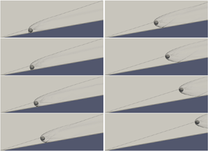
The present two-part work is concerned with studying a simplified version of such a separation problem, in which the parent geometry is represented by a two-dimensional ramp and the shed object by a spherical body of uniform density. To provide a well-defined initial condition for the shed body, we limit ourselves to the situation in which it lies on the ramp with zero initial velocity and is released instantaneously into the flow. Although somewhat idealized, the problem as studied captures much of the key physics of the situations described above, and we thus expect it to give insight into more realistic scenarios. We illustrate this problem in the sequence of numerical schlieren images in figure 1, taken from an inviscid free-flight simulation with a ramp angle of 10 $^\circ$ and a free-stream Mach number of 6. In this example, the ramp-generated oblique shock initially intersects the sphere's bow shock just above the sphere, and in the resulting trajectory the sphere appears to ride the shock downstream. Our objective is to characterize such sphere trajectories as the Mach number, ramp angle and starting position along the ramp are varied, for both inviscid and viscous flows. The inviscid case is the focus of the present article; the effects of flow viscosity are examined in Part 2 (Butler et al. Reference Butler, Whalen, Sousa and Laurence2021).

Figure 1. Numerical schlieren images of a sphere being shed from a 10 $^\circ$ ramp in a Mach-6 inviscid flow.
In figure 1, it is clear that there are two distinct phases to the sphere trajectory: at earlier times the sphere is affected by the near-wall flow created by its interaction with the ramp itself, but at later times only by the external ramp flow (and in this particular case, the ramp-generated shock). We first summarize what can be expected of the later phase based on the literature to date. To begin, note that this part of the trajectory will depend very little on whether the flow is viscous or inviscid, as the forces on a blunt body in high-speed flow are dominated by pressure components. If the sphere is immersed entirely within either the shock layer or the free-stream flow, the dynamics will be rather trivial as they will be determined purely by the drag force in that respective region (in the corresponding flow direction). If the sphere is interacting with the shock itself, however, the situation becomes more interesting. The detailed flow structures created when an oblique shock impinges on the bow shock generated by a blunt body were first elucidated by Edney (Reference Edney1968a,Reference Edneyb), who identified six qualitatively different shock–shock interaction patterns (denoted type I to type VI). The aerodynamic forces that are produced on a spherical geometry when exposed to such interactions were examined by Laurence & Deiterding (Reference Laurence and Deiterding2011), who also used these results to predict the dynamical behaviour of a sphere interacting with an isolated planar oblique shock. Cases were examined in which the sphere is initially stationary and released upstream of or on the shock; it was found that there are a range of initial conditions for which the sphere ‘surfs’ the shock downstream, i.e. moves along the shock while oscillating about a stable point lying at a fixed location relative to the shock. This behaviour is possible because the maximum lift-to-drag ratio of the sphere as it interacts with the shock can exceed the tangent of the shock angle. From a vehicle standpoint then, one concern in the current context may be that the shock generated at the leading edge would act as a guide to channel particles towards (or away from) particular regions.
In contrast to the interaction of the sphere with the oblique shock, the initial phase of sphere separation from the wall will be highly dependent on whether the fluid is inviscid or viscous, as the presence of a ramp boundary layer will significantly alter the flow field near the wall. We assume for the time being that this near-wall flow is unaffected by the ramp shock (this will be a reasonable assumption in cases such as that shown in figure 1, for which the sphere starts from an appreciable distance downstream of the leading edge). For an inviscid flow, the ramp wall will act simply as a reflecting boundary condition, and the near-wall flow will be exactly the same as if the wall were replaced by a second, mirroring sphere. The separation of such identical blunt bodies from one another has been studied in the context of meteoroid fragmentation. Artem'eva & Shuvalov (Reference Artem'eva and Shuvalov1996) performed numerical simulations and found that the normalized separation (transverse) velocity of two hemi-cylinders once separation was complete was  $V'_T = \sqrt {\rho _b/\rho _a}V_T/V \approx 0.2$, where
  $V_T$ is the dimensional transverse velocity of each object,
  $V$ is the free-stream velocity and
  $\rho _b$ and
  $\rho _a$ are the densities of the bodies and the atmosphere. Laurence, Parziale & Deiterding (Reference Laurence, Parziale and Deiterding2012) conducted both experiments and simulations of separating spheres at Mach 4, and found that
  $V'_T=0.24$. Further investigations of this or similar problems have been carried out, for example, by Park & Park (Reference Park and Park2020) and Register et al. (Reference Register, Aftosmis, Stern, Brock, Seltner, Willems, Guelhan and Mathias2020). In such configurations, the mutual repulsion of the two bodies is caused by the confined, high-pressure region that develops between them when they are closely spaced. If a boundary layer is present on the ramp, however, the resulting flow field will be much more complicated, as the sphere bow shock will produce a shock-wave/boundary-layer interaction (SWBLI) where it impinges upon the wall. We might thus expect the forces on the sphere in the presence of an SWBLI to be quite different from the inviscid case, which in turn will affect the sphere dynamics; such viscous effects will be the focus of Part 2.
For the present article, the main implication of the inviscid approximation will be to neglect the boundary layer that develops on the ramp, and therefore any interactions between this and the flow around the sphere. This approximation will thus become increasingly realistic in the limit of the sphere radius being much larger than the ramp boundary-layer thickness. Neglecting the ramp boundary layer here will enable us to explore a wider range of ramp angles and free-stream Mach numbers than would otherwise be possible; nevertheless, much of the insight gained (especially in cases where the sphere/shock effects are dominant) can be expected to carry over to the viscous scenario.
In the inviscid separation event of figure 1, the sphere is repulsed away from the ramp wall in the initial part of its trajectory; this is a result of both the wall and shock interactions. In this example, we note that even though the influences of both these interactions are present at early times, they are effectively decoupled from one another since they affect different regions of the sphere surface. Such decoupling will generally hold unless the sphere is initially positioned close to the leading edge of the ramp. Therefore, in the following analysis, we consider first the sphere–shock interactions (§ 3) and then the sphere–wall interactions (§ 4) independently of one another, before examining their combined influence on the sphere dynamics in § 5. Additional effects are investigated in § 6 before conclusions are drawn. To begin, however, we describe the numerical approach employed.
2. Numerical methodology
As in Laurence & Deiterding (Reference Laurence and Deiterding2011), we employ the Cartesian fluid solver framework AMROC (Deiterding Reference Deiterding2003, Reference Deiterding2011; Ziegler et al. Reference Ziegler, Deiterding, Shepherd and Pullin2011) to simulate numerically the interaction of a spherical body with a two-dimensional ramp. The equations solved to model the inviscid compressible fluid are the Euler equations in conservation-law form
 \begin{align} \partial_t \rho + \boldsymbol{\nabla}\!\boldsymbol{\cdot}(\rho \boldsymbol{u}) = 0, \enspace \partial_t (\rho \boldsymbol{u}) + \boldsymbol{\nabla}\boldsymbol{\cdot}(\rho \boldsymbol{u}\otimes\boldsymbol{u}) + \boldsymbol{\nabla} p = 0, \enspace \partial_t (\rho E) + \boldsymbol{\nabla}\boldsymbol{\cdot}((\rho E+p)\boldsymbol{u}) = 0. \end{align}
Here,  $\rho$ is the fluid density,
  $\boldsymbol {u}$ the velocity vector and
  $E$ the specific total energy. The hydrostatic pressure
  $p$ is given by the polytropic gas equation,
  $p = (\gamma -1)(\rho E - \frac {1}{2}\rho \boldsymbol {u}^T\boldsymbol {u})$, where
  $\gamma$ is the ratio of specific heats. We approximate (2.1a–c) in three spatial dimensions using a discretely conservative Cartesian finite-volume discretization built on dimensional splitting. The flux vector splitting approach by Van Leer is used to evaluate an upwinded numerical flux at cell interfaces; the monotonic upstream-centred scheme for conservation laws (MUSCL)-Hancock reconstruction technique with Minmod-limiter is employed to construct a high-resolution method that is of second-order approximation accuracy away from shocks and contact discontinuities, cf. Deiterding (Reference Deiterding2003).
The spherical bodies are represented on the Cartesian mesh with a scalar level-set function,  $\varphi$, that stores the signed distance to the nearest point on either sphere surface to each finite-volume cell centre. For non-overlapping spheres, the evaluation of
  $\varphi$ is straightforward and we adopt the convention
  $\varphi >0$ in the fluid domain and
  $\varphi <0$ inside the solid bodies. By utilizing the sign of
  $\varphi$, the first layer of cells inside each body can be identified; the vector of state in these cells is then adjusted to model the relevant non-Cartesian boundary conditions, i.e. a rigid sphere moving with velocity
  $\boldsymbol {v}$, before applying the unaltered Cartesian finite-volume discretization. The last step involves the interpolation and mirroring of
  $\rho$,
  $\boldsymbol {u}$, and
  $p$ across the sphere boundary and the modification of the normal velocity in the immersed boundary cells to
  $(2\boldsymbol {v}\boldsymbol {\cdot }\boldsymbol {n}-\boldsymbol {u}\boldsymbol {\cdot }\boldsymbol {n})\boldsymbol {n}$, with
  $\boldsymbol {n}=\boldsymbol {\nabla }\varphi /|\boldsymbol {\nabla }\varphi |$, cf. Deiterding (Reference Deiterding2009). The benefit of this immersed boundary, aka ‘ghost fluid’ method (Fedkiw et al. Reference Fedkiw, Aslam, Merriman and Osher1999) is the natural incorporation of moving bodies. However, the approach usually reduces the approximation accuracy along the immersed boundary, in the present implementation to first order. We mitigate this error by applying automatic, dynamic mesh adaptation along
  $\varphi =0$ and additionally to important flow features, specifically to gradients larger than a certain threshold in the fluid density. The adopted mesh adaptation method is the recursive block-structured algorithm for explicit finite-volume discretizations after Berger & Colella (Reference Berger and Colella1988), allowing simultaneous adaptive mesh refinement (AMR) in time and space by the same factor,
  $l_j$, for each additional level
  $j$. In AMROC, the AMR method is fully parallelized for distributed memory machines, including automatic load balancing and parallel re-partitioning as the mesh refinement hierarchy changes throughout a computation (Deiterding Reference Deiterding2005).
In the simulations described hereinafter, the sphere and ramp surface are always fully enveloped by cells at the highest level of mesh adaptation, and no exchange of kinetic energy by direct contact is allowed to take place. The hydrodynamic force,  $\boldsymbol {f}$, on the sphere is updated after every highest-level time step by integrating the pressure over the body surface, for the purpose of which spherical longitude–latitude grids are temporarily constructed. The position of the sphere's centre,
  $\boldsymbol {x}$, is then updated by advancing the equation of motion,
  $\ddot {\boldsymbol {x}}=\boldsymbol {f}/m$, with mass
  $m=\frac {4}{3}{\rm \pi} r^3\rho _b$ (
 $r$ being the sphere radius and
  $\rho _b$ its density). Finally, the level-set function is re-calculated.
This inviscid computational approach has been applied and experimentally validated in our earlier work on high-speed interactions between two spheres (Laurence Reference Laurence2006; Laurence, Deiterding & Hornung Reference Laurence, Deiterding and Hornung2007; Laurence et al. Reference Laurence, Parziale and Deiterding2012). The present sphere–ramp geometry is somewhat simpler and includes just a single moving body; we can thus expect the methodology to provide accurate and reliable results.
Two different categories of simulations were employed within this general framework. The first was free-flight simulations, in which the initial sphere velocity was zero and the sphere density was typically set to a value such that the sphere would traverse the computational domain of interest while typically maintaining a velocity that was negligible compared to that of the free stream. An example of such a simulation is shown in figure 1; here, the sphere velocity remains below 2.5 % of the free stream throughout the simulation. One such computation, however, can only provide information about a single initial condition, and as such, free-flight simulations were primarily performed to analyse the sphere dynamics near the ramp leading edge (§ 5.3), where the approximations used elsewhere (as described in § 5.1) become tenuous. In such simulations, a typical base grid was  $60 \times 40 \times 20$ (physical dimensions
  $3.0 \times 2.0 \times 1.0$), with three levels of additional refinement, each of factor two. The sphere diameter was 0.4 in physical units, which corresponded to 64 cells at the finest level. The sphere velocity remained below 0.5 % of the free stream in all simulations investigating the leading-edge behaviour.
The second category of simulation we refer to as ‘forced’, in that the sphere density was set to an artificially high value and an impulsive velocity was imparted on the sphere once the flow over it had been established; thus, the sphere traced out a prescribed straight-line trajectory that was not influenced by the aerodynamic forces. In this way the aerodynamic forces as functions of the position relative to the ramp wall or shock could be characterized in an efficient manner. Two sub-categories of forced simulations were performed. In the first, the ramp was present and the sphere was started with a lateral velocity from an initial position either touching the ramp (if a characterization of the aerodynamic influences from both the ramp wall and shock was desired, as in § 5.1) or out in the shock layer (if only the influence of the shock was of interest, as in § 3). The sphere velocity in the forced sphere-ramp simulations was generally 1.5 % of the free-stream velocity. A typical computation had a base grid of  $280 \times 90 \times 20$ cells (
 $14.0\times 4.0 \times 1.0$ in physical units), with three levels of additional refinement, each of factor two. The sphere diameter was 0.5 physical units, corresponding to 80 cells at the finest level – this was found to be sufficiently resolved for converged force calculations (results of a mesh refinement study involving such a forced simulation are provided in § 3). Such a computation would typically require
  $\sim$1800 CPU hours on 20 Intel Xeon cores, including both the flow start-up period and the time for sphere traversal. In some cases, a refinement factor of four at only the highest level was used to improve the quality of flow visualization, while additional simulations with only two levels of additional refinement were used to fill out the relevant parameter space in § 3 and § 5.
In the second sub-category of forced simulations, the angle of the ramp was set to zero, and the ramp thus acted simply as a reflecting wall boundary condition. The sphere was again traversed normal to the free-stream flow (this time with a lateral velocity of 0.7 % of the free-stream value). The base grid was  $60\times 30 \times 50$ cells, with three levels of additional refinement (factor two); the sphere diameter was again 80 cells at the finest level. Such simulations were performed to explore the interaction of the sphere solely with the ramp surface and will be described in further detail in § 4.
In all inviscid simulations, the fluid was a perfect gas with a ratio of specific heats of 1.4 (unless otherwise stated). The Courant–Friedrichs–Lewy (CFL) number ranged from 0.6 to 0.95, the lower value being necessary to maintain numerical stability at higher Mach numbers.
3. Interactions between a sphere and an oblique shock
In an earlier work (Laurence & Deiterding Reference Laurence and Deiterding2011), two of the present authors discovered a phenomenon referred to as ‘shock-wave surfing’, whereby it is possible for a sphere to follow a stable trajectory downstream along a planar oblique shock. Since the main focus of that earlier work was the interaction between two spheres, only a brief description of the ramp-sphere case was given; for the present work, it is instructive to both review this surfing phenomenon and examine it in further detail.
To begin, a sequence of flow visualizations from a forced sphere-ramp simulation is shown in figure 2. Here, the free-stream Mach number is 6 and the ramp angle,  $\theta$, is 10
 $^\circ$. The lateral position of the sphere centre (
 $y$) is varied while the streamwise location (
 $x$) remains constant (with the origin of the coordinate system being the leading edge of the ramp). A numerical schlieren (magnitude of the density gradient) on the plane through the sphere centre is visualized at each time step, along with a colour map showing contours of pressure on the surface of the sphere. Corresponding drag and lift coefficients (
 $C_D$ and
  $C_L$) are plotted in figure 3(a) (high refinement curve); here, the abscissa is the lateral distance from the sphere centre to the extrapolated location of the oblique shock at the streamwise location of the sphere centre (
 $y_s = x\tan \beta$, where
  $\beta$ is the shock angle), normalized by the sphere radius. Force coefficients are calculated based on the free stream rather than post-shock conditions. We observe that the drag coefficient decreases essentially monotonically as the sphere passes from inside to outside the shock layer. The lift coefficient has a finite, positive value inside the shock layer (because of the non-zero flow angle behind the shock), increases further as the sphere passes through the shock, reaches a maximum value at
  $y$ slightly below
  $y_s$, and then decreases again as the sphere moves out into the free stream. The small non-zero value of
  $C_L$ in the free stream is a result of the finite lateral velocity of the sphere; for a stationary sphere,
  $C_L$ would of course be zero here. The increase in
  $C_L$ during interaction with the shock is caused primarily by the lower side of the sphere being exposed to doubly shocked flow, which results in a higher pressure than the singly shocked flow on the upper side of the sphere.

Figure 2. Numerical schlieren images with pressure contour maps on the surface of the sphere as it interacts with the oblique shock generated by a 10 $^\circ$ ramp at Mach 6. The pressure scale is different for each visualization.

Figure 3. (a) Drag (upper curves) and lift (lower curves) coefficients computed for a sphere as its position is varied relative to the shock generated by a 10 $^\circ$ ramp at Mach 6 for a range of refinement levels: (
 $\cdots$) coarse; (– –) medium; (–
  $\cdot$ –
  $\cdot$ –) medium-high; (—) high. (b) Lift-to-drag ratio as the sphere position is varied at Mach 6 (–
  $\cdot$ –
  $\cdot$ –), 10 (– –) and 20 (—). For each curve,
  $\tan \beta$ is indicated by the horizontal dotted line. The symbols on the Mach-6 curve indicate the locations of the visualizations in figure 2.
As the force coefficients are integrated quantities, they are relatively insensitive to the grid resolution. To demonstrate this, in figure 3(a) we also show curves derived from three other numerical simulations with different total levels of refinement: the coarse through medium–fine simulations have one through three levels of additional refinement over the base grid, each of factor two, while the fine simulation (referred to previously) has a refinement factor of four only at the third additional level. Each simulation is thus effectively twice as resolved as the one before. Although some small changes are noted as we move from coarse to medium–fine, the medium–fine and fine results are essentially identical. To conserve computational resources then, medium–fine refinement was used for the bulk of the force characterization described in this section, while the highly refined simulations were used primarily for flow visualization in a few select cases, such as that shown in figure 2. In these highly refined simulations, a smaller computational domain was used with the sphere located further upstream than in the force-characterization simulations.
The lift-to-drag ratio ( $L/D$) of the sphere as it is translated through the shock is shown in the right part of figure 3, together with corresponding curves for two other Mach numbers. To reduce the effects of the sphere motion on the calculated forces (primarily the lift, as the drag is largely unaffected), the lift profile used to calculate this curve has been shifted so that the free-stream value is zero, and scaled such that
  $L/D$ is equal to the tangent of the ramp angle when the sphere is fully immersed in the shock layer. The points in this simulation corresponding to the visualizations of figure 2 are indicated by symbols on the curve. The maximum
  $L/D$ ratio,
  $(L/D)_{max}$, occurs when the sphere is experiencing a type-IV Edney interaction (second visualized time step). Changes in the slope of the
  $L/D$ curve are generally observed at transitions between shock–shock interaction types (e.g. type-III to type-II near the penultimate visualized time step) or when other qualitative changes in the flow field take place (e.g. the shear layer generated in the type-III interaction moving off the sphere surface in the fourth visualized time step). Also shown is a dotted horizontal line indicating the value of
  $\tan \beta$ for this Mach number. The maximum
  $L/D$ is seen to be larger than
  $\tan \beta$ in this case, and
  $L/D$ is equal to
  $\tan \beta$ at two values of
  $(y-y_s)/r$. Both of these locations will therefore be stationary points, i.e. if the sphere is released at either of those points with zero velocity, it will remain at the same value of
  $(y-y_s)/r$ as it moves downstream; however, the slope of the
  $L/D$ curve tells us that only the outer point will be a stable one (see Laurence & Deiterding (Reference Laurence and Deiterding2011) for further discussion).
Similar curves for Mach numbers of 10 and 20 (again for  $\theta =10^\circ$) are also shown in figure 3(b). We see that the degree to which the maximum
  $L/D$ exceeds the tangent of the shock angle increases substantially as the Mach number is increased. This is a result of both a decreasing
  $\tan \beta$ (for a fixed
  $\theta$) and an increasing
  $(L/D)_{max}$; the former effect is well-known oblique shock behaviour, while the second we shall return to shortly. The distance between the two stationary points also increases with Mach number.
As was shown in Laurence & Deiterding (Reference Laurence and Deiterding2011), to analyse the sphere dynamics it is instructive to utilize the reduced coordinates  $\eta =(y-y_s)/r$ and
  $v_\eta =\textrm {d}\eta /\textrm {d}\hat {t}=\hat {v}_y-\tan \beta \,\hat {v}_x$, with
  $\hat {v}_x = \sqrt {\rho _b/\rho _a}v_x/V$,
  $\hat {v}_y = \sqrt {\rho _b/\rho _a}v_y/V$ and
  $\hat {t}=\sqrt {\rho _a/\rho _b}Vt/r$. We can then reduce the original four equations of motion to the following two-equation system:
 \begin{gather} \frac{\textrm{d}\eta}{\textrm{d}\hat{t}} = v_\eta, \end{gather}
 \begin{gather}\frac{\textrm{d} v_\eta}{\textrm{d} \hat{t}} = \frac{3}{8}\left[ C_L(\eta) - \tan\beta C_D(\eta) \right]. \end{gather}
This allows a phase-plane analysis to be employed to describe the sphere dynamics, with trajectories obtained by integrating the combined equation
 \begin{equation} \frac{\textrm{d} v_\eta}{\textrm{d} \eta} = \frac{3(C_L - \tan\beta C_D)}{8v_\eta}, \end{equation}
giving
 \begin{equation} v_\eta^2 = \tfrac{3}{4}\int (C_L - \tan\beta C_D) \, \textrm{d} \eta. \end{equation}
Note that by writing  $C_L$ and
  $C_D$ as functions solely of
  $\eta$ (and not of sphere velocity), we are assuming that the sphere velocity remains negligible in comparison to the free stream throughout the time period of interest. Phase diagrams of the sphere motion for a Mach-6 free stream and ramp angles of 5
 $^\circ$, 10
 $^\circ$, and 20
 $^\circ$ are shown in figure 4. For the smallest ramp angle, there are no stationary points: in this case, the maximum value of the lift-to-drag ratio is smaller than
  $\tan \beta$, which precludes the possibility of the sphere following the shock downstream. Therefore, all sphere trajectories eventually lead to the sphere becoming entrained inside the shock layer. Increasing the ramp angle to 10
 $^\circ$ brings about a qualitative change in the phase portrait. Now the maximum L/D is greater than
  $\tan \beta$ and two stationary points appear on the phase diagram: the inner (
 $\eta <0$), unstable point is a saddle, while the outer (
 $\eta >0$), stable point is a centre. The separatrix to the right of the saddle point is a closed curve that forms the boundary of all stable orbits about the centre. Increasing the ramp angle to 20
 $^\circ$ does not bring about a qualitative change in the phase portrait, although we see that the stable region becomes more extended along both the
  $\eta$ and
  $v_\eta$ axes. Manipulating the coefficient curves revealed that the extent of the stable region in the
  $v_\eta$ dimension is directly related to the degree by which
  $(L/D)_{max}$ exceeds
  $\tan \beta$.

Figure 4. Phase diagrams of the sphere behaviour for a Mach-6 free stream and ramp angles of (a) 5 $^\circ$, (b) 10
 $^\circ$ and (c) 20
 $^\circ$. Separatrices are shown by dashed lines.
One point regarding (3.3) that will become important is that if  $v_\eta =0$,
  $\textrm {d} v_\eta /\textrm {d} \eta$ is infinite (unless
  $C_L = \tan \beta C_D$), and therefore trajectories starting from rest will initially trace out vertical lines in the phase plane (except those that begin exactly at stationary points). We also note that, for
  $\eta \lesssim -1, C_D$ is constant and
  $C_L = C_D \tan \theta$ (as the sphere is fully immersed inside the shock layer). In this case we can directly integrate equation (3.4) to obtain
 \begin{equation} v_\eta^2 = c - \tfrac{3}{4}(\tan\beta - \tan\theta) C_D \eta, \end{equation}
 $c$ being a constant of integration. We thus see that these parts of the sphere trajectories in the phase plane are parabolas. Similarly, for
  $\eta \gtrsim 1$ (outside the shock),
  $C_D$ is constant and
  $C_L =0$, and the trajectories are parabolas of the form
 \begin{equation} v_\eta^2 = c - \tfrac{3}{4}\tan\beta C_D \eta. \end{equation}
 In figure 5 we have graphed the phase-plane separatrices for ramp angles of 5 $^\circ$, 10
 $^\circ$ and 20
 $^\circ$, in each case for Mach numbers of 6, 10 and 20. The most consistent trend observed is that increasing
  $M$ enlarges the stable region in the phase plane along both axes. At Mach 6 and 10, increasing the ramp angle to 20
 $^\circ$ similarly extends the stable region along both axes, but the corresponding effect at Mach 20 is not so clear: the extent in the
  $\eta$ dimension is in fact maximum for 5
 $^\circ$, whereas the
  $v_\eta$ extent grows (if modestly) up to 20
 $^\circ$. To the left of the saddle point, the slope of the separatrix becomes shallower as the Mach number is increased, and steeper as the ramp angle is increased.

Figure 5. Separatrices of the phase diagrams for a sphere interacting with a ramp-generated oblique shock for ramp angles of (a) 5 $^\circ$, (b) 10
 $^\circ$ and (c) 20
 $^\circ$, in each case for free-stream Mach numbers of (– –) 6, (—) 10 and (–
  $\cdot$ –
  $\cdot$ –) 20. The symbols indicate the centre locations for (
 $+$) Mach 6, (
 $\times$) Mach 10 and (
 $\circ$) Mach 20.
The effects of varying  $\theta$ and
  $M$ on the stationary-point locations are shown more explicitly in figure 6. In panel (a),
  $\theta$ is varied for Mach numbers of 6, 10 and 20, whereas in (b),
  $M$ is varied for each of
  $\theta =5^\circ$, 10
 $^\circ$ and 20
 $^\circ$. The location of the centre is relatively unaffected by the ramp angle, but does change more substantially with
  $M$, being pushed out to larger
  $\eta$ as
  $M$ is increased. The saddle point, on the other hand, shows a weak general trend to more negative
  $\eta$ as both
  $M$ and
  $\theta$ are increased. The net result is that the spacing between the two stationary points grows with increasing
  $M$, but remains relatively constant as
  $\theta$ is varied.

Figure 6. Locations of (unfilled symbols) saddle point and (filled symbols) centre (a) as the ramp angle is varied at constant  $M$ (
$M$ ( $\triangle$, 6;
  $\circ$, 10;
  $\square$, 20) and (b) as
  $M$ is varied for a several ramp angles (
 $\triangle$, 5
 $^\circ$;
  $\circ$, 10
 $^\circ$;
  $\square$, 20
 $^\circ$).
As we will see, the slope of the separatrix at the saddle point is an important parameter in determining the separation behaviour; this value can be determined from (3.3). Noting that both the numerator and denominator are zero at the saddle point, we use l'Hôpital's rule to obtain
 \begin{equation} \left.\frac{\textrm{d} v_\eta}{\textrm{d} \eta}\right|_{sp} = \pm \sqrt{\frac{3}{8}[C_L'(\eta_{sp}) - \tan\beta C_D'(\eta_{sp}) ]}, \end{equation}
where the subscript  $sp$ refers to the saddle point. For the Mach-6 phase portraits, this slope takes the values of 0.41 and 0.62 for 10
 $^\circ$ and 20
 $^\circ$ ramps; at Mach 10, the values are 0.48, 0.73 and 0.80 for 5
 $^\circ$, 10
 $^\circ$ and 20
 $^\circ$ ramps. We thus observe that this slope tends to increase with both Mach number and ramp angle, but remains somewhat below unity for the cases considered.
We noted earlier that the source of the large lift coefficients generated as the sphere moves through the shock is the difference in pressures resulting from the singly shocked flow on the upper surface and the doubly shocked flow on the lower surface. We finish the present section by examining this effect in more detail. In Laurence & Deiterding (Reference Laurence and Deiterding2011), it was noted that a reasonable approximation to the lift and drag curves could be obtained if it were assumed that the oblique shock effectively divided the flow over the sphere into two regions of Newtonian flow. Then the local pressure coefficient is  $C_p = C_p^*\sin ^2\theta$, where
  $\theta$ is the angle between the local surface element and the incoming flow, and
  $C_p^*$ is a reference pressure coefficient, which according to the modified Newtonian theory of Lees (Reference Lees1955), will simply be the Pitot pressure in the relevant flow region. An examination of the Pitot pressure upstream and downstream of the ramp-generated oblique shock should thus provide some understanding of the lift behaviour of the sphere.
Formulae for the ratios of Pitot pressure across an oblique shock in terms of the shock angle and Mach number are given by Graham & Davis (Reference Graham and Davis1965) for cases in which the post-shock flows are both subsonic and supersonic. In figure 7(a) we have plotted this ratio,  $p_{t2}/p_{t1}$, against the ramp angle for Mach numbers of 6, 10 and 20. We see that
  $p_{t2}/p_{t1}$ reaches a maximum on the weak-shock branch at a ramp angle that decreases from 23.1
 $^\circ$ for Mach 6 to 15.3
 $^\circ$ for Mach 20. The peak value of
  $p_{t2}/p_{t1}$ increases with
  $M$, and would reach a maximum of 6 for
  $M = \infty$,
  $\theta =0$. At a very basic level, we might thus expect the peak
  $C_L$ of the sphere to increase with
  $M$ for a given
  $\theta$ and, for a given Mach number (within the range considered in the present work), to occur at an angle somewhere in the range of 15–25
 $^\circ$. In figure 7(b), we have plotted this peak,
  $C_{L,max}$, versus ramp angle for the same Mach numbers, as computed in the forced numerical simulations. We do indeed observe a monotonic increase in
  $C_{L,max}$ with Mach number and although
  $C_{L,max}$ is increasing with
  $\theta$ over the range plotted, for
  $M=20$ it does appear to be approaching a maximum near
  $\theta =25^\circ$. The peak
  $L/D$ values from these simulations are also plotted on the same axes. We see that these again increase monotonically with Mach number, although the curves do not appear to be approaching a maximum with
  $\theta$ (this is because the drag values at peak
  $L/D$ begin to decrease with
  $\theta$). Nevertheless, we conclude that a simple consideration of the Pitot pressures before and after the oblique shock gives significant insight into the prevalence of surfing over a range of conditions.

Figure 7. (a) Ratio of Pitot pressure before and after obliques shocks with varying turn angle for Mach numbers of (- $\blacktriangle$-) 6, (-
 $\bullet$-) 10 and (-
 $\blacksquare$-) 20. The weak-shock branch in each case is indicated by the solid curve with symbols, the corresponding strong-shock branch by the dashed curve. (b) Computed maximum lift coefficient (closed symbols) and maximum lift-to-drag ratio (open symbols) as functions of ramp angle for a sphere interacting with an oblique shock for Mach numbers of (-
 $\blacktriangle$-) 6, (-
 $\bullet$-) 10 and (-
 $\blacksquare$-) 20.
4. Near-wall aerodynamics
It is clear from the first two images of figure 1 that the presence of the ramp significantly alters the flow over the lower part of the sphere, in particular, by maintaining a stronger shock down to the ramp wall. This increases the pressure on the lower half of the sphere, leading to a repulsive force that propels the sphere out towards the ramp-generated oblique shock. If the near-wall part of the flow field is free from the influence of the oblique shock, as we have assumed thus far, variation of just two flow parameters – the Mach number behind the oblique shock and the wall-normal displacement of the sphere – is sufficient to fully characterize such near-wall aerodynamic effects. Therefore, we may elucidate these effects by considering the simpler problem of a sphere separating from a reflecting, inviscid wall aligned with the incoming flow.
We performed forced simulations of a sphere translating away from a reflecting wall boundary at various Mach numbers, as described in § 2. Figure 8 shows the computed flow fields at different stages during the sphere–wall separation for Mach numbers of 3 and 12. The flow field development is seen to be qualitatively similar in the two cases. When the sphere is in contact with the wall, the sphere bow shock extends down to the wall with little decrease in strength; the flow ahead of the lower part of the sphere is then entirely subsonic and generates high pressure levels on the sphere surface. As the sphere translates away from the wall, the flow between the sphere and the wall accelerates to supersonic conditions, resulting in first a Mach throat and then a three-dimensional regular reflection. The reflected shock initially impinges on the lower sphere surface, causing a local increase in pressure, but once the shock moves off the rear of the sphere, the presence of the wall has negligible further influence on the sphere aerodynamics (the only effect possible being to modify the wake flow). For the higher Mach number, the bow shock lies closer to the sphere and the transitions between these different flow configurations occur at smaller values of  $y/r$: for example, in the second image showing the Mach reflection for the Mach-3 sequence (figure 8b), the sphere is at
  $y/r=1.39$, while for the corresponding Mach-12 image (figure 8e), the sphere is at
  $y/r=1.15$.

Figure 8. Sequences of numerical schlieren slices and pressure contours on the sphere as it is translated away from an inviscid wall in (a–c) Mach-3 and (d–f) Mach-12 free-stream flows.
In figure 9 we plot the lift and drag coefficients as functions of normalized wall-normal distance for Mach numbers of 3, 6, 10 and 14. In the lift-coefficient profiles (note that these have been shifted vertically so that they asymptote to zero, in order to remove the influence of the wall-normal motion), we observe that the lateral force in each case decreases monotonically as the sphere moves away from the wall. The maximum lift value increases slightly as the Mach number increases (from 0.259 for  $M=3$ to 0.277 for
  $M=14$), but much more significant is the extended range of
  $y/r$ over which the influence of the wall is felt at lower Mach numbers. For
  $M=14$,
  $C_L$ drops below 0.005 at
  $y/r=1.44$, while for
  $M=3$, this does not occur until
  $y/r=1.64$. The sphere drag is moderately enhanced through being in close proximity to the wall, increasing by approximately 20 % compared to the uninfluenced value in the free stream. For each Mach number, the drag initially decreases as the sphere moves away from the wall, then undershoots slightly before rising to the free-stream value; this undershoot occurs when the reflected shock from the wall impinges towards the rear of the sphere, increasing the back-side pressure. The effect of increasing Mach number is to decrease the overall drag coefficient and limit the
  $y/r$ range over which the sphere is influenced, as with the lift.

Figure 9. (a) Lift and (b) drag coefficients of a near-wall sphere as functions of normalized distance from the wall, for Mach numbers of (- $\blacktriangle$-) 3, (-
 $\blacksquare$-) 6, (-
 $\blacklozenge$-) 10 and (-
 $\bullet$-) 14.
The effects of these Mach number trends on the sphere parameters once separated from the wall are summarized in figure 10, where we plot the normalized wall-normal distance,  $y_{sep}/r$, at which the lift coefficient has fallen to 1 % of its maximum value, as well as the normalized sphere velocities at this point (e.g.
  $\hat {v}_{y,sep} = \sqrt {\rho _b/\rho _a}v_{y,sep}/V$, where
  $v_{y,sep}$ is the physical
  $y$ velocity at
  $y_{sep}$), versus the Mach number. The velocities are obtained by integrating the force-coefficient profiles; note that
  $\hat {v}_{y,sep}$ is identical to the normalized separation velocity,
  $V'_T$, discussed in the introduction. As would be expected from the discussion of the previous paragraph, all plotted separation parameters (
 $y_{sep}/r$,
  $\hat {v}_{y,sep}$ and
  $\hat {v}_{x,sep}$) decrease with increasing Mach number, falling rapidly at first but then more gradually as the Mach number increases above
  $\sim$4. Despite the enhanced lateral impulse the sphere receives at lower Mach numbers, the angle at which it is travelling once it escapes the influence of the wall increases slightly as the Mach number rises (from 8.6
 $^\circ$ at
  $M=2$ to 10.4
 $^\circ$ at
  $M=14$). Comparing
  $C_L$ and
  $C_D$ at
  $y/r=1$ in figure 9, it is clear that this trend also holds true for the initial direction of travel.

Figure 10. Parameters of the sphere motion when it is effectively free of wall influence (the subscript  $sep$ refers to the point at which the lift coefficient has decreased to 1 % of its maximum value): (a) separation distance,
  $y_{sep}/r$; (b,c) normalized lateral and streamwise velocities at
  $y_{sep}/r$.
Ultimately we are interested in how this behaviour will affect the separation of the sphere from a ramp oriented at a non-zero angle to the free stream. Each of the forced sphere–wall computations allows us to simulate a range of sphere-ramp separation cases, all sharing their post-shock Mach number with the free-stream value in the relevant computation (but through different combinations of free-stream Mach number and ramp angle to achieve this). The trajectory of the sphere in  $\eta{-}v_\eta$ space in these simulated separation events will then provide insight into how this initial wall interaction affects the possibility of subsequent surfing in the full separation problem. In figure 11(a), we present such phase-plane trajectories for a 10
 $^\circ$ ramp and three free-stream Mach numbers (
 $M=6.59$, 8.49 and 14.30, corresponding to post-shock Mach numbers of 5, 6 and 8); the abscissa here is the change in
  $\eta$, since the initial value of
  $\eta$ is arbitrary. To obtain these trajectories, the sphere–wall force-coefficient curves are integrated and then rotated;
  $\rho _a$ and
  $V$ are then rescaled (in calculating
  $v_\eta$) based on the oblique-shock relations. For the reason noted in discussing (3.3), all trajectories start off vertically, but then curve around as the influence of the wall diminishes, resulting in a peak
  $v_\eta$ in all cases. This peak increases notably with increasing Mach number, and typically occurs when
  $v_\eta$ is of the same order of or slightly larger than
  $\Delta \eta$. In figure 11(b), we show phase-plane trajectories for a fixed free-stream Mach number of 10 and various ramp angles. The trajectories are all of a similar shape, but the trend with
  $\theta$ is non-monotonic insofar as the 16.2
 $^\circ$ trajectory reaches a higher value of
  $v_\eta$ than those of either the smaller or larger ramp angles. Overall, however, the influence of the ramp angle on the phase-plane trajectory is somewhat less than that of the Mach number (at least over the range of parameters considered here).

Figure 11. Initial sphere trajectories in the  $\eta$–
 $v_\eta$ phase plane produced by isolated wall interactions: (a) for
  $\theta =10^\circ$ and free-stream Mach numbers of (—) 6.59, (– –) 8.49 and (–
  $\cdot$ –
  $\cdot$ –) 14.30; (b) for
  $M=10$ and ramp angles of (—) 5.85
 $^\circ$, (– –) 12.24
 $^\circ$, (–
  $\cdot$ –
  $\cdot$ –) 16.18
 $^\circ$ and (
 $\cdots$) 21.40
 $^\circ$.
We can explore the trends in the value of  $v_\eta$ following separation in more detail by interpolating the data shown in figure 10 to determine the value of
  $v_\eta$ once separation from the wall is complete – which we denote
  $v_{\eta ,sep}$ (note from figure 11 that this will be slightly lower than the peak value of
  $v_\eta$) – for varying ramp angles and Mach numbers. We do this by following a procedure similar to that just described for the trajectories in figure 11, i.e. a rotation of the interpolated values of
  $v_{x,sep}$ and
  $v_{y,sep}$ followed by a rescaling of the density and velocity to calculate
  $v_{\eta ,sep}$. In figure 12(a),
  $v_{\eta ,sep}$ is plotted versus Mach number for ramp angles of 5
 $^\circ$, 10
 $^\circ$, 15
 $^\circ$, 20
 $^\circ$ and 25
 $^\circ$, and in figure 12(b) versus the ramp angle for free-stream Mach numbers of 6, 8, 10, 12, 16 and 20. For all ramp angles,
  $v_{\eta ,sep}$ increases monotonically with Mach number; this we can attribute primarily to the decreasing shock angle (for a given
  $\theta$) as the Mach number is increased, together with a small contribution from the increase in the angle of the sphere velocity relative to the wall noted earlier. In contrast, the trend with
  $\theta$ (for fixed
  $M$) is non-monotonic, with
  $v_\eta$ attaining a maximum at a ramp angle that decreases with increasing Mach number (generally between
  $\theta =10^\circ$ and 15
 $^\circ$).

Figure 12. Normalized shock relative velocity when the sphere is free of the wall influence: (a) versus Mach number for ramp angles of (— $\blacktriangle$—) 5
 $^\circ$, (—
 $\blacksquare$—) 10
 $^\circ$, (—
 $\blacklozenge$—) 15
 $^\circ$, (—
 $\bullet$—) 20
 $^\circ$ and (—
 $\blacktriangledown$—) 25
 $^\circ$; and (b) versus ramp angle for Mach numbers of (—
 $\blacktriangle$—) 6, (—
 $\blacksquare$—) 8, (—
 $\blacklozenge$—) 10, (—
 $\bullet$—) 12, (—
 $\blacktriangleleft$—) 16 and (—
 $\blacktriangleright$—) 20.
Before proceeding further, let us consider how the behaviour observed thus far is likely to affect the possibility of surfing. We note that the trends for the sphere–wall separation in the present section in some way reflect those seen in the extent of the stable surfing region in § 3. In particular, for fixed  $\theta$, the stable region contracts with decreasing Mach number; however, since the effective repulsion from the wall interaction (in terms of
  $v_\eta$) is also reduced as the Mach number is decreased, we might expect these effects to counteract one another (to some extent) when considering the full separation problem. Also, if the ramp angle is increased from zero for fixed
  $M$, both the extent of the stable region and the wall repulsion increase to a maximum before falling again. Again, these two effects would be expected to work against one another with regard to enabling stable surfing trajectories. Which of these effects are dominant, however, remains to be seen.
5. Full separation behaviour
5.1. Decoupled force model
Having investigated the aerodynamic interactions of the sphere with the ramp-generated shock and ramp wall independently, we are now in a position to examine the full separation behaviour. To allow complete sphere trajectories to be calculated in an efficient manner, a decoupled approach based on forced simulations was developed as follows. For a given  $M$ and
  $\theta$, force-coefficient data were generated for sphere positions from the ramp surface out into the free stream. The streamwise sphere location in each of these simulations was chosen such that there was a finite intermediate region over which the sphere was free from the influence of both the wall and the shock, and thus the coefficients were constant, say,
  $C_{Di}$ and
  $C_{Li}$. The force coefficients as functions of
  $y/r$ for such a simulation with
  $M=10$ and
  $\theta =10^\circ$ are shown in figure 13(a); in this case
  $x/r=48$ and the boundaries of the intermediate region are indicated by dashed lines. For any larger
  $x/r$, the coefficient profiles will be identical except that the intermediate region will be stretched as a result of the increased distance between the wall and shock (which will grow as
  $[\tan \beta -\tan \theta ]x$). For smaller
  $x/r$, this intermediate region will shrink until a critical value,
  $x_c/r$, is reached at which its extent is exactly zero. If we decrease
  $x/r$ further from this critical point, the sphere will begin to experience the effects of the oblique shock before it is free from the wall influence. Nevertheless, as we have noted earlier, these two effects will be largely independent of one another unless the sphere is very close to the leading edge; this means their combined influence on the force coefficients will be additive. Thus, if
  $x<x_c$, we modify the parts of the coefficient curves over which the sphere is influenced by both the shock and the wall in the following way (illustrated in figure 13b). For the drag, let
  $\Delta C_{Dw}$ be the additional increment in the drag coefficient compared to
  $C_{Di}$ produced by the influence of the wall at a given
  $y$ location (as calculated from the original
  $C_D$ curve); similarly, let
  $\Delta C_{Ds}$ be the increment (compared to
  $C_{Di}$) at that
  $y$ produced by the interaction with the oblique shock. The total drag coefficient is then calculated simply as
  $C_D=C_{Di}+\Delta C_{Dw}+\Delta C_{Ds}$, and similarly for
  $C_L$. In this way the forces experienced by the sphere anywhere in the flow field can be well approximated, with the exception of locations close to the leading edge (just how close to the leading edge this decoupled assumption is valid will be examined in § 5.3). Thus, for any initial sphere position, we can integrate the equations of motion and derive the resulting sphere trajectory. Again, the assumption that the sphere velocity remains negligible in comparison to the free-stream flow is required here (since
  $C_L$ and
  $C_D$ are assumed to be functions solely of the sphere position).

Figure 13. (a) Full force-coefficient curves (—,  $C_D$; –
  $\cdot$ –
  $\cdot$ –,
  $C_L$) including wall- and shock-affected regions for
  $M=10, \theta =10^\circ$; the vertical dashed lines indicate the boundaries of the region over which the sphere is free from the influence of both the wall and the shock, and the dotted line is the shock location (
 $y_s$). (b) Construction of composite curve using the decoupled model for values of
  $x/r$ for which the wall and shock simultaneously influence the sphere; the wall-only and shock-only parts of the original curve are plotted in dashed and dashed-dotted lines, respectively.
5.2. Sphere trajectories with the decoupled model
Example trajectories for a ramp angle of 10 $^\circ$ and a Mach number of 10 are shown in figure 14. Those trajectories for which the sphere is shed further upstream (
 $x_0/r \leq 15$) appear to exhibit stable surfing; for
  $x_0/r=36$ the sphere is clearly entrained within the shock layer, while for
  $x_0/r=25$ and 32 its fate is less clear. The corresponding phase-plane trajectories for these cases are shown in figure 15(b). Here we see that for
  $x_0/r=9$, 11, 13, and 15, the sphere does indeed attain an orbit within the stable region of the phase diagram. For
  $x_0/r=25$ and 32, the initial repulsion from the wall takes the sphere trajectory above the upper branch of the separatrix – the sphere will thus temporarily move outside the shock layer but will subsequently re-enter and become entrained within. If the initial position of the sphere is shifted further rearwards (e.g.
  $x_0/r=36$), it will simply become entrained without first exiting the shock. We can generalize to say that one of these three categories of trajectories – stable surfing, temporary escape/ejection followed by re-entrainment or direct entrainment – will be the fate of any spherical body shed from a ramp. Ejection/re-entrainment trajectories are only possible (for initially stationary spheres) because of the repulsive influence of the ramp interactions, whereas the other two trajectory types would be possible for an isolated oblique shock without any direct ramp influence. What remains to determine then is how the boundaries of
  $x_0/r$ delineating these behaviours vary for different free-stream Mach numbers and ramp angles. For combinations of Mach number and ramp angle for which there is no stable region (e.g. the Mach-6,
  $\theta =5^\circ$ case shown in figure 4a), ejection/re-entrainment and direct entrainment will be the only possibilities, but there will be no distinct boundary between the two.

Figure 14. Calculated separation trajectories for a Mach 10 free stream and a ramp angle of 10 $^\circ$; the starting positions are
  $x_0/r=9$, 11, 13, 15, 25, 32 and 36.

Figure 15. Separation trajectories in the phase plane for a Mach 10 free stream with ramp angles of: (a) 5 $^\circ$,
  $x_0/r=9$, 11, 13, 15, 25, 32 and 36; (b) 10
 $^\circ$,
  $x_0/r=9$, 11, 13, 15, 25, 32 and 36; (c) 20
 $^\circ$,
  $x_0/r=9$, 11, 13, 15, 21 and 25. In each case, the trajectory that corresponds to the largest
  $x_0/r$ is the one that originates from the minimum value of
  $\eta$ on the
  $v_\eta =0$ axis. Separatrices are shown in dashed lines.
Some insight into the effect of varying the ramp angle can be gained by comparing the graph just described with the other two of figure 15, which show phase-plane trajectories for angles of 5 $^\circ$ and 20
 $^\circ$ (at Mach 10). We see in both cases the limiting
  $x_0/r$ for stable surfing is shifted forward, with only the
  $x_0/r=9$ case of those plotted producing a stable orbit. This is despite the extent of the stable region along the
  $v_\eta$ coordinate being significantly larger for
  $\theta =20^\circ$ than for
  $\theta =10^\circ$.
For Mach-6 trajectories at ramp angles of 10 $^\circ$, 15
 $^\circ$ and 20
 $^\circ$, figure 17 demonstrates that there is in fact no possibility of stable surfing according to the decoupled model, with all sphere trajectories being pushed outside the stable boundary during the wall-separation phase (figure 16 shows the trajectories in physical space for
  $\theta =10^\circ$). In contrast, for the Mach-20 trajectories with
  $\theta =5^\circ$, 10
 $^\circ$ and 20
 $^\circ$ (figure 18), a wide range of initial locations can produce surfing, especially for the smaller ramp angles.

Figure 16. Calculated separation trajectories for a Mach 6 free stream and a ramp angle of 10 $^\circ$; the starting positions are
  $x_0/r=5$, 7, 9, 11, 13, 15.5 and 17.
In general, we observe from figures 15, 17, and 18 that, for surfing to be initiated, the sphere must initially lie within the stable region of the phase plane. In discussing figure 11 it was noted that the sphere–wall interactions impart a combination of  $\Delta v_\eta$ and
  $\Delta \eta$ that is somewhat steeper than the slope of the separatrix near the saddle point. As a result, there is no way for the wall interaction to push the sphere trajectory into the stable region if it begins outside (the opposite tendency rather prevailing). Therefore, if
  $\eta _0$ is the initial value of
  $\eta$,
  $\eta _0\geq \eta _{sp}$ is a necessary (but not sufficient) condition for surfing, and thus surfing trajectories are only possible if the ramp-generated oblique shock is initially incident on the sphere.

Figure 17. Separation trajectories in the phase plane for a Mach 6 free stream with ramp angles of: (a) 10 $^\circ$,
  $x_0/r=5$, 7, 9, 11, 13, 15.5 and 17; (b) 15
 $^\circ$,
  $x_0/r=5$, 7, 9, 11, 13, 15 and 17; (c) 20
 $^\circ$,
  $x_0/r=5$, 7, 9, 11, 13, 13.5 and 15.

Figure 18. Separation trajectories in the phase plane for a Mach 20 free stream with ramp angles of: (a) 5 $^\circ$,
  $x_0/r=15$, 23, 31, 33, 65, 95 and 100; (b) 10
 $^\circ$,
  $x_0/r=13$, 19, 25, 27, 45, 65 and 70; (c) 20
 $^\circ$,
  $x_0/r=9$, 11, 13, 14, 22, 28 and 33.
5.3. Sphere dynamics near the ramp leading edge
The decoupled force model will not be a good approximation close to the leading edge of the ramp, as there the shock–shock interactions will affect the lower part of the sphere and thus the flow in the vicinity of the wall, in violation of our decoupled assumption. This is clear from figure 19(a), which shows the flow field over a sphere at the surface of a 10 $^\circ$ ramp with
  $x/r=5$ in a Mach-6 free stream. The shock–shock interaction produces a complex flow pattern near the wall, with a Mach stem extending to the ramp surface and a localized region of very high pressure on the underside of the sphere. This is quite different from the near-wall flow field effectively assumed in the decoupled model, of which the first image in figure 1 is representative.

Figure 19. (a) Numerical schlieren image of a sphere sitting on a 10 $^\circ$ ramp in a Mach-6 free stream at a distance downstream of
  $x/r=5$; pressure contours on the sphere surface are also shown. (b) Comparison of the initial part of the sphere trajectory for this starting location as predicted by the decoupled model (– –) and in the free-flight simulation (—).
In order to obtain more accurate predictions for such upstream starting locations, as well as to verify that the decoupled model performs well elsewhere, free-flight simulations were conducted for a range of initial sphere positions (but concentrating on cases relatively close to the leading edge). The initial part of the trajectory in physical space for the case shown in figure 19(a)  $(M=6, \theta =10^\circ , x_0/r=5)$ is compared with the decoupled prediction in (b). The free-flying sphere leaves the wall at a steeper angle than the decoupled model predicts, as the localized high-pressure region on the underside of the sphere generates higher lift than in the decoupled model (with little difference in drag). As the sphere moves away from the wall, however, the free-flight trajectory curves around more sharply than the decoupled one, leading to a shallower angle of travel at later times. This is a result of the shock–shock interaction displacing the high-pressure region on the underside of the sphere downstream, meaning that although the lift coefficient is initially higher than in the decoupled prediction, it drops off rapidly as the sphere moves away from the wall. The overall influence of the sphere–wall interaction is thus decreased.
With these observations in mind, in figure 20 we compare free-flight and decoupled trajectories in the phase plane for a 10 $^\circ$ ramp at Mach 10, as well as 10
 $^\circ$ and 15
 $^\circ$ ramps at Mach 6. In all three graphs, for starting locations near or upstream of the centre, the overprediction of the wall repulsion just noted results in decoupled trajectories that are pushed out to larger
  $v_\eta$ values than those of the free-flying spheres. For
  $M=10, \theta =10^\circ$, this discrepancy does not modify the qualitative behaviour, although the decoupled model will slightly underpredict the
  $x_0/r$ value at which the transition from surfing to ejection/re-entrainment occurs. Similarly, for
  $M=6, \theta =10^\circ$, no change in qualitative behaviour is noted for the free-flight trajectories compared to the decoupled ones, despite the reduced wall repulsion; in particular, surfing is still not possible for any starting location. For
  $M=6, \theta =15^\circ$, however, the free-flight simulations show that there is in fact a range of near-leading-edge initial positions for which surfing is possible (
 $x_0/r \lesssim 5$), contrary to the predictions of the decoupled model. For all three Mach-number/ramp-angle combinations considered here, the decoupled model provides accurate predictions for starting locations with
  $\eta _0 \lesssim 0$.

Figure 20. Trajectories near the leading edge for: (a) Mach 10, 10 $^\circ$ ramp and initial sphere locations of
  $x_0/r=5$, 9, 13, 17 and 21; (b) Mach 6, 10
 $^\circ$ ramp and initial sphere locations of
  $x_0/r=3$, 5, 7, 9 and 11; (c) Mach 6, 15
 $^\circ$ ramp and initial sphere locations of
  $x_0/r=3$, 5, 7, 9 and 11. In each case, the solid lines show the results of free-flight simulations and the dot-dashed lines indicate the predicted trajectory from the decoupled force model.
Our objective in the following subsection is to use the decoupled model to determine how the transition boundaries between the different trajectory types vary with Mach number and ramp angle; the comparisons just made provide a means to gauge how accurate these predictions will be. First, we note that the ejection/re-entrainment to direct entrainment boundary will be well predicted, given that this transition occurs when  $\eta _0<\eta _{sp}$, which will always be sufficiently far downstream that the decoupled assumption is valid. The trajectories in figure 20 show that the transition
  $x_0/r$ from surfing to ejection/re-entrainment will be slightly underpredicted by the decoupled model (and, in cases where surfing is marginal, may be erroneously predicted not to exist). Nevertheless, as this underprediction appears to be consistent across ramp angle and Mach number (at least for the cases examined), we may still expect that the trends predicted by the model to be accurate.
5.4. Boundaries of sphere behaviour
From decoupled trajectory predictions such as those shown in figures 15, 17 and 18, for a given  $M$ and
  $\theta$ it is straightforward to determine the critical values of
  $x_0/r$ at which the sphere behaviour transitions between the different categories – surfing, ejection/re-entrainment, direct entrainment – with the minor caveats mentioned in the previous paragraph. In figure 21 we plot these boundaries in
  $x_0/r$–
 $\theta$ space for Mach numbers of 6, 10, and 20 (a) and in
  $x_0/r$–
 $M$ space for ramp angles of 5
 $^\circ$, 10
 $^\circ$, and 20
 $^\circ$ (b). In (a), we see that the transition between surfing and ejection/re-entrainment at Mach 10 exhibits a relatively weak dependence on
  $\theta$ for ramp angles between 5
 $^\circ$ and 25
 $^\circ$. The trend is not monotonic, but rather the transition
  $x_0/r$ increases to a maximum of 14.0 for
  $\theta =10^\circ$ as the ramp angle is increased, before gradually decreasing to reach
  $x_0/r=7.6$ at
  $\theta =25^\circ$. The maximum range of initial locations leading to surfing is thus found near
  $\theta =10^\circ$. For
  $M=20$, the surfing to ejection/re-entrainment transition
  $x_0/r$ is larger and the curve is shifted to lower
  $\theta$, with the maximum
  $x_0/r$ now occurring near or below
  $\theta =5^\circ$. For both Mach 10 and Mach 20, the ejection/re-entrainment to direct entrainment boundary shows the same qualitative behaviour as the surfing to ejection/re-entrainment boundary at the same Mach number, just shifted to larger
  $x_0/r$. For
  $M=10$, the range of
  $x_0/r$ for ejection/re-entrainment is maximum at
  $\theta \approx 7.5^\circ (13.1\leq x_0/r \leq 33.6)$. For
  $M=20$, the range of
  $x_0/r$ over which this behaviour is observed reaches a maximum (of the ramp angles simulated) of
  $32.3 \leq x_0/r \leq 98.3$ at
  $\theta =5^\circ$. The corresponding
  $M=6$ curve (note that there is no surfing to ejection/re-entrainment boundary at this Mach number) is somewhat flatter and shifted to smaller
  $x_0/r$; the maximum here is
  $x_0/r=15.7$ at
  $\theta =10^\circ$.

Figure 21. Boundaries between regions of different sphere behaviours: (a) in  $x_0/r$–
 $\theta$ space for Mach numbers of (
 $\blacktriangle$) 6, (
 $\circ$,
  $\bullet$) 10 and (
 $\square$,
  $\blacksquare$) 20; (b) in
  $x_0/r$–
 $M$ space for ramp angles of (
 $\triangle$,
  $\blacktriangle$) 5
 $^\circ$, (
 $\circ$,
  $\bullet$) 10
 $^\circ$ and (
 $\square$,
  $\blacksquare$) 20
 $^\circ$. Open symbols with dashed lines indicate transitions from surfing to ejection/re-entrainment, and closed symbols with solid lines indicate transitions from ejection/re-entrainment to direct entrainment.
Figure 21(b) shows how these transition boundaries vary with Mach number. The most obvious trend is that both transition boundaries shift to larger  $x_0/r$ as Mach number is increased. For
  $\theta =20^\circ$, there is little change above
  $M=16$, behaviour which might be expected from the Mach number independence principle (Anderson Reference Anderson2006); however, for
  $\theta =10^\circ$ and especially for
  $\theta =5^\circ$, the transition
  $x_0/r$ values are still increasing significantly at
  $M=20$. In general then, the range of
  $x_0/r$ over which both surfing and ejection/re-entrainment are possible will increase with Mach number, especially for small ramp angles.
One factor that has not been considered thus far, but will certainly influence the  $x_0/r$ values plotted in figure 21, is the initial lateral distance from the sphere centre to the shock. We have noted that surfing is only possible if the shock is initially impinging on the sphere, and if the shock angle is larger relative to the ramp angle, the sphere will need to be located further upstream to produce such a flow configuration. In figure 22 we plot the quantity
  $\tan \beta -\tan \theta$, i.e. the lateral separation between ramp and shock at unit distance downstream of the leading edge, versus the ramp angle. As would be expected, this quantity decreases with Mach number; however, perhaps less intuitively, we see that the minimum for a given (finite)
  $M$ is reached at non-zero
  $\theta$, which shifts closer to zero as
  $M$ is increased. We note that the minima in the Mach 6, 10 and 20 curves in figure 22 fall at roughly the same angles as the corresponding extrema in figure 21(a), which may indicate that the initial sphere–shock spacing plays an important role here.

Figure 22. Lateral distance between shock and ramp at unit distance downstream for Mach numbers of (uppermost to lowermost curve) 4, 6, 8, 10, 15, 20.
As an aside, since the  $\theta$ values for minimum separation in figure 22 are small and the Mach numbers of interest large, the corresponding shock angles will also be small and we can approximate
  $\tan \beta -\tan \theta \approx \tan (\beta -\theta )$. Differentiating the oblique-shock relation
 \begin{equation} \tan(\beta-\theta)=\tan\beta\frac{(\gamma-1)M_1^2\sin^2\beta+2}{(\gamma+1)M_1^2\sin^2\beta}, \end{equation}
it is straightforward to show that  $\tan (\beta -\theta )$ has a minimum when
 \begin{equation} \tan\beta=\left(1+\frac{\gamma-1}{2}M^2\right)^{-1/2}. \end{equation}
No such simple relation is known by the authors for the minimum in  $\tan \beta -\tan \theta$.
In figure 23 we replot the boundary curves of figure 21 but now versus the normalized initial lateral distance from the sphere centre to the shock,  $\eta _0 = (y_0-y_s)/r$. This successfully collapses much of the data for the surfing to ejection/re-entrainment transition boundary; indeed, we see that the value of
  $\eta _0$ for this transition is close to constant (
 $\eta _0 \approx 0$) over the range of cases considered, with discrepancies only for small ramp angles and lower Mach numbers. We thus conclude that the dynamical behaviour of the sphere as it transitions from surfing to ejection/re-entrainment is determined primarily by the initial lateral location of the sphere relative to the shock, regardless of Mach number and ramp angle. This suggests that it is the sphere–shock interactions (rather than the sphere–wall interactions) that are most important in determining the sphere dynamics in this region of the parameter space. The ejection/re-entrainment to direct entrainment boundaries, in contrast, are poorly collapsed by this scaling, for variations in both ramp angle and Mach number. The main Mach number trend observed here is that the transition
  $\eta _0$ becomes more negative, i.e. the sphere lies further inside the shock, as the Mach number is increased (and more rapidly for smaller
  $\theta$). The trend with ramp angle depends on the specific Mach number, but we do see that for large ramp angles, the boundary appears to be asymptoting to
  $\eta _0 \approx -1.5$ (from above for low
  $M$ and from below for high
  $M$). The poor collapse of the data for this boundary points to the increased significance of the initial sphere–wall interactions compared to the surfing to ejection/re-entrainment boundary.

Figure 23. Boundaries between regions of different sphere behaviours: (a) in  $(y_0-y_s)/r$–
 $\theta$ space for Mach numbers of (
 $\blacktriangle$) 6, (
 $\circ$,
  $\bullet$) 10 and (
 $\square$,
  $\blacksquare$) 20; (b) in
  $(y_0-y_s)/r$–
 $M$ space for ramp angles of (
 $\triangle$,
  $\blacktriangle$) 5
 $^\circ$, (
 $\circ$,
  $\bullet$) 10
 $^\circ$ and (
 $\square$,
  $\blacksquare$) 20
 $^\circ$. Open symbols with dashed lines indicate transition from surfing to ejection/re-entrainment and closed symbols with solid lines indicate transition from ejection/re-entrainment to direct entrainment.
6. Additional effects
6.1. Influence of non-negligible sphere velocity
In all results derived from the forced simulations, we have effectively assumed that the aerodynamic forces experienced by the sphere are independent of the sphere velocity, which will be appropriate if this remains a negligible fraction of the flow velocity. Similarly, in the free-flight simulations presented thus far, we have specified the sphere density such that this would be the case. In a more realistic situation, however, as the sphere accelerates downstream the assumption of negligible sphere velocity will become increasingly tenuous. It is of interest then to evaluate the effects of finite velocity on the sphere dynamics, and in particular how the surfing phenomenon is affected. To this end, a set of free-flight simulations was conducted on an extended domain (150 sphere radii in downstream extent) in which the sphere density was varied so as to achieve a range of sphere velocities with otherwise identical computational parameters. In all cases the Mach number was 10 and the ramp angle 10 $^\circ$. To make such large-domain simulations feasible, the degree of refinement was reduced to a single level of factor two above the base grid (equivalent to the coarse computation in figure 3). Although this will have some influence on the force coefficients compared to the better-resolved simulations, we expect the effects of finite sphere velocity to be consistent within this set and representative of such effects overall. Results from these simulations are shown as phase-plane trajectories in figure 24. Three starting locations close to the boundary between surfing and ejection/re-entrainment were chosen (
 $x_0/r=13$, 14 and 15) and the sphere density was varied by a factor of sixteen (
 $\rho _b/\rho _a=21.4\times 10^3, 5.36\times 10^3$ and
  $1.34\times 10^3$), resulting in sphere velocities towards the downstream end of the computational domain of typically 8 %, 16 % and 29 % of the free-stream velocity. The effects of such sphere velocities on the surfing behaviour is seen to be limited. For the largest sphere density, the qualitative behaviour is exactly the same as if the sphere velocity was entirely negligible, with the
  $x_0/r=13$ and 14 trajectories stably surfing (despite the
  $x_0/r =14$ trajectory temporarily leaving the stable region) and the
  $x_0/r =15$ trajectory exhibiting expulsion/re-entry. For
  $\rho _b/\rho _a=5.36\times 10^3$, the
  $x_0/r=14$ trajectory has now (just) transitioned from surfing to expulsion/re-entry, while the other two remain qualitatively unchanged; this remains the case when the sphere density is again decreased to
  $\rho _b/\rho _a=1.34\times 10^3$. We note that for hypersonic flight at
  $30$ km altitude and assuming a sphere density of
  $6\times 10^3$ kg m
 $^{-3}$ (typical of high-temperature ceramics), we will have
  $\rho _b/\rho _a \approx 3.3 \times 10^5$; the finite-velocity effects on surfing seen here would thus only manifest themselves a substantial distance further downstream than was simulated. We conclude that a non-negligible sphere velocity may decrease the prevalence of surfing, but its effects will be limited and generally only become important hundreds of sphere radii downstream.

Figure 24. Phase trajectories for  $M=10, \theta =10^\circ$ showing the effect of non-negligible sphere velocity on the sphere behaviour. In each case the starting locations are
  $x_0/r=13$, 14 and 15, and the sphere densities are set such that the maximum streamwise sphere velocities are approximately (a) 8 %, (b) 16 % and (c) 29 % of the free stream.
6.2. Variable ratios of specific heats
Thus far we have assumed that the fluid is a perfect gas with a constant ratio of specific heats of  $\gamma =1.4$. As the free-stream Mach number increases, however, high-temperature effects (primarily vibrational excitation and molecular dissociation) will emerge (Anderson Reference Anderson2006) and this perfect-gas assumption will become increasingly inaccurate. A detailed examination of these effects is beyond the scope of this paper, but at least a qualitative estimate of how they will affect the sphere dynamics is possible through considering variations in the ratio of specific heats. Activation of the internal energy modes will decrease the effective
  $\gamma$ towards unity; approximating high-temperature effects through variations in
  $\gamma$ is thus common in the literature (see, for example, Gnoffo et al. Reference Gnoffo, Weilmuenster, Braun and Cruz1996). To begin, we note that decreasing
  $\gamma$ will reduce the shock angle for a given
  $\theta$, and from this alone we would expect the transition boundaries between the categories of sphere behaviour to be shifted to larger
  $x_0/r$; however, changes in
  $\gamma$ will also affect both the sphere–shock and sphere–wall interactions, and we consider these briefly now.
Regarding sphere–shock interactions, we noted earlier in our discussion of figure 7 that the maximum  $L/D$ that the sphere experiences as it passes through the shock is closely linked to the ratio of pressures before and after the oblique shock, and that this in turn dictates the surfing behaviour (i.e. the existence and size of the stable surfing region). In figure 25(a) we have plotted the ratio of Pitot pressures across a Mach-10 oblique shock against the ramp angle for values of
  $\gamma$ from 1.1 to 1.4. For a fixed
  $\theta$, this Pitot-pressure ratio increases with decreasing
  $\gamma$, and the maximum value over the range of possible
  $\theta$ also increases: for
  $\gamma =1.1$, this maximum is more than double that for
  $\gamma =1.4$. Based on our earlier arguments then, we would expect the maximum sphere
  $L/D$ to increase as
  $\gamma$ is decreased. In figure 25(b), which shows the sphere
  $L/D$ versus
  $(y-y_s)/r$ for forced simulations with
  $\gamma$ values of 1.2 and 1.4 (both for
  $M=10, \theta =10^\circ$), we see that this is indeed the case. As a result, the stable region in the phase plane is larger for
  $\gamma =1.2$ compared to
  $\gamma =1.4$, and we can generalize to predict this as a consistent trend.

Figure 25. (a) Ratio of Pitot pressure before and after an oblique shock with varying turn angle for a Mach number of 10 and ratios of specific heat of (- $\blacktriangle$-) 1.1, (-
 $\blacksquare$-) 1.2, (-
 $\blacklozenge$-) 1.3 and (-
 $\bullet$-) 1.4. The weak-shock branch in each case is indicated by the solid curve with symbols, the corresponding strong-shock branch by the dashed curve. (b) Lift-to-drag ratio for a sphere as it is translated through the oblique shock created by a 10
 $^\circ$ ramp at Mach 10 for (– –)
  $\gamma =1.2$ and (—)
  $\gamma =1.4$.
As for the effect of decreasing the ratio of specific heats on the sphere–wall interactions, a series of forced simulations similar to those described in § 4 were performed with varying  $\gamma$. As
  $\gamma$ tends towards unity, the bow shock around the sphere moves closer to the sphere surface, which decreases the value of
  $y_{sep}/r$ (i.e. the wall-normal distance at which the wall effects on the forces become negligible), and thus also the net repulsion that the sphere experiences from the wall. Overall then, decreasing
  $\gamma$ would be expected to promote the likelihood of surfing for a given Mach number and ramp angle. This is confirmed in figure 26, which shows phase-plane trajectories for
  $M=10, \theta =10^\circ$, and ratios of specific heats of
  $\gamma =1.2$, 1.3 and 1.4, all with the same
  $x_0/r$ values (note that the
  $\gamma =1.4$ case is the same as figure 15b). Clearly, decreasing
  $\gamma$ shifts the transition boundaries downstream, expanding the range of
  $x_0/r$ for which surfing and ejection/re-entrainment will occur. For example, the
  $x_0/r=15$ trajectory is ejected just outside the stable region for
  $\gamma =1.4$, but remains inside for
  $\gamma =1.3$, and even more so for
  $\gamma =1.2$.

Figure 26. Separation trajectories in the phase plane for a Mach 10 free stream, a ramp angle of 10 $^\circ$ and ratios of specific heats of (a) 1.4, (b) 1.3 and (c) 1.2. The starting locations are
  $x_0/r=9$, 11, 13, 15, 25, 32 and 36 (as in figure 15b).
We finally note that the trends observed in this section (pertaining to both finite sphere velocities and high-temperature effects) can be expected to carry over to viscous scenarios.
7. Conclusions
In this first of a two-part work, we have examined the dynamical behaviour of a sphere released suddenly into a hypersonic inviscid flow from the surface of a planar ramp. A variety of numerical simulations were performed to investigate the separation behaviour. Forced simulations, in which the aerodynamic forces acting on the sphere along a specified trajectory were computed, were used to study the interactions first between the sphere and the ramp-generated oblique shock and then between the sphere and the ramp wall itself. The sphere–shock simulations provided insight into the conditions under which shock-wave surfing – a phenomenon in which the sphere rides the oblique shock downstream – is possible for different free-stream Mach numbers and ramp angles. This was facilitated by a phase-plane analysis that showed that the size of the stable region associated with surfing increases monotonically with increasing free-stream Mach number; however, the trend with ramp angle was less clear. For the sphere/ramp-wall interactions, forced simulations were conducted of a sphere translating away from a wall aligned with the free-stream flow (i.e. zero ramp angle); results were then extrapolated to finite ramp angles with the same post-shock Mach numbers (equal to the free-stream value in the corresponding simulation). The wall exerts a repulsive force on the sphere, and this is felt further away from the wall as the local Mach number is reduced. Nevertheless, as the free-stream Mach number is increased for a given ramp angle, the wall interactions result in an increased tendency for the sphere to be expelled out of the stable surfing region in the phase plane.
To enable full sphere trajectories to be simulated in a computationally efficient manner, a decoupled model was developed in which the influences of both shock and wall interactions contributed to the overall sphere forces, but were assumed to act independently of one another. Predictions from the model were compared to results from free-flight simulations, with generally good agreement except when the sphere was released close to the ramp leading edge. Three types of sphere trajectories were found to be possible: in order of increasing distance of release from the ramp leading edge these were (i) surfing of the sphere down the shock, (ii) initial expulsion from the shock layer followed by re-entry and entrainment or (iii) direct entrainment inside the shock layer. At Mach 6, the decoupled model predicted surfing to be unattainable because of the tendency of the wall interaction to push the sphere trajectory outside of the stable region in the phase plane (though free-flight simulations showed that surfing was in fact possible for a very limited range of ramp angles and release locations). At lower hypersonic Mach numbers then, type (ii) and (iii) trajectories are predominant. By raising the Mach number, however, surfing becomes possible over an increasing range of ramp angles and sphere release locations. This demonstrates that, in terms of Mach number trends, the enlargening of the stable region in the phase plane with increasing Mach number is more significant for the sphere behaviour than the increased wall-induced expulsion. In all cases, however, the nature of the wall interaction is to expel the sphere trajectory from the stable region of the phase plane rather than bring it inside, meaning that the sphere must initially lie within the stable region for surfing to be initiated.
The decoupled model was used to predict the transition boundaries (in terms of the downstream release location,  $x_0/r$) between the different trajectory types as functions of the free-stream Mach number and ramp angle. For large Mach numbers and small ramp angles, the range of initial sphere locations over which surfing and ejection/re-entrainment occur can become quite large; however, it should be noted that in such cases the ramp boundary layer would become very thick, resulting in pronounced viscous interactions and making the inviscid assumption increasingly untenable, even for large sphere radii. The observed trends were clearly linked to the spacing between the oblique shock and the ramp surface at the release location, which motivated recasting the transition boundaries in terms of the initial lateral sphere displacement from the shock. This re-parameterization was found to give a good collapse of the type (i) to (ii) transition boundary, but was less successful in collapsing the type (ii) to (iii) boundary data.
We noted in the introduction that, from a hypersonic-vehicle standpoint, one concern associated with the surfing phenomenon may be that the leading-edge shock would guide shed particles preferentially towards downstream parts of the vehicle. Based on our present findings, we expect that this concern should be more significant at higher Mach numbers, and that particles shed very close to the leading edge are most likely to follow such trajectories. Indeed, it is also closest to the leading edge that heating levels are highest and we might thus surmise that particulate shedding is most likely to occur. Alternatively, it may be possible to take advantage of the surfing phenomenon to direct shed objects away from vulnerable parts of the vehicle.
As a closing observation, we note clear parallels between the separation behaviour here and that observed for two spheres in Laurence & Deiterding (Reference Laurence and Deiterding2011) and Laurence et al. (Reference Laurence, Parziale and Deiterding2012). In the earlier works, as the secondary (smaller) sphere size was increased, the behaviour transitioned from entrainment within the shock layer of the primary (larger) sphere, to an increased tendency to surf the primary shock downstream, to expulsion of the secondary sphere from the primary shock layer beyond a critical radius ratio. This behaviour is clearly mirrored in the present work as the sphere release location is moved progressively closer to the ramp leading edge. The primary difference in behaviours arises from the constant shock angle in the present case. This means that the force-coefficient profiles resulting from the sphere–shock interactions are unchanging as the sphere moves downstream, allowing clear distinctions between the trajectory types that are not possible in the two-sphere case.
Future work might consider shedding from a non-planar parent body. An axisymmetric configuration, for example, would have a decreased shock angle for the equivalent final deflection angle and, as we have seen in the current study, a shallower shock angle increases the likelihood of surfing. Additionally, it may be of interest to examine the effects of sudden or gradual changes in ramp angle on sphere trajectories. Such geometrical changes are characteristic of scramjet intakes (see, for example, the X-43 vehicle), and might in some cases cause a jump from one trajectory type to another. Finally, non-spherical geometries for the shed body may exhibit behaviour distinct from that found in the present study, especially if rotations play a significant role.
Declaration of interests
The authors report no conflict of interest.


