


1 Introduction
Problems involving particle–fluid interactions are widely encountered in different applications, such as sediment transport, air pollution, the pharmaceutical industry, blood flow, and petrochemical and mineral processing plants. Controlling heat transfer in particulate suspensions also has many important applications, such as packed- and fluidized-bed reactors and industrial dryers. In these cases, in addition to momentum and/or mechanical interactions between particles and fluid, the flow is also characterized by heat transfer between the two phases. Owing to the complex phenomena related to the diffusion and convection of heat in particulate flows, a better understanding of the heat transfer between the two phases in the presence of a flow is essential to improve the current models. The aim of this study is to validate the proposed numerical algorithm against existing experimental and numerical studies and then to examine, in particular, the effect of finite particle inertia and the difference in fluid- and solid-phase thermal diffusivity on the heat transfer across a sheared particle suspension. Ensemble-averaged equations are derived to disentangle the heat transfer in the fluid and solid phases.
Simplified theoretical approaches and experiments have been used previously to study these challenging physical phenomena. The experiments of Ahuja (Reference Ahuja1975) on sheared suspensions of polystyrene particles at finite particle Reynolds numbers (
 $Re_{p}>1$
) revealed a significant enhancement of heat transfer. The author attributed this enhancement to a mechanism based on the inertial effects, in which the fluid around the particle is centrifuged by the particle rotation. Sohn & Chen (Reference Sohn and Chen1981) investigated the eddy transport, associated with microscopic flow fields in shearing two-phase flows with volume fraction of spherical particles up to
$Re_{p}>1$
) revealed a significant enhancement of heat transfer. The author attributed this enhancement to a mechanism based on the inertial effects, in which the fluid around the particle is centrifuged by the particle rotation. Sohn & Chen (Reference Sohn and Chen1981) investigated the eddy transport, associated with microscopic flow fields in shearing two-phase flows with volume fraction of spherical particles up to
 $30\,\%$
. At low Reynolds numbers and high Péclet numbers
$30\,\%$
. At low Reynolds numbers and high Péclet numbers
 $Pe$
, they found an increase in the heat transfer, which approaches a power-law relationship with
$Pe$
, they found an increase in the heat transfer, which approaches a power-law relationship with
 $Pe$
. The Péclet number
$Pe$
. The Péclet number
 $Pe$
defines the ratio between fluid viscosity and heat diffusivity in the fluid. Chung & Leal (Reference Chung and Leal1982) measured experimentally the effective thermal conductivity of a sheared suspension of rigid spherical particles. These authors compared their results to the theoretical prediction of Leal (Reference Leal1973) for a sheared dilute suspension at low particle Péclet number,
$Pe$
defines the ratio between fluid viscosity and heat diffusivity in the fluid. Chung & Leal (Reference Chung and Leal1982) measured experimentally the effective thermal conductivity of a sheared suspension of rigid spherical particles. These authors compared their results to the theoretical prediction of Leal (Reference Leal1973) for a sheared dilute suspension at low particle Péclet number,
 $Pe$
, reporting good agreement. In addition, they investigated moderate concentrations (volume fraction
$Pe$
, reporting good agreement. In addition, they investigated moderate concentrations (volume fraction
 $\unicode[STIX]{x1D719}<25\,\%$
) and higher Péclet numbers compared to the study by Leal (Reference Leal1973). It was later suggested by Zydney & Colton (Reference Zydney and Colton1988) that the increase in solute transport, previously observed for particle suspensions, is caused by shear-induced particle diffusion (Madanshetty, Nadim & Stone Reference Madanshetty, Nadim and Stone1996; Breedveld et al.
Reference Breedveld, Van Den Ende, Bosscher, Jongschaap and Mellema2002) and the resulting dispersive fluid motion. These authors proposed a model, based on existing experimental results, concluding that the augmented solute transport is expected to vary linearly with the Péclet number. Shin & Lee (Reference Shin and Lee2000) experimentally studied the heat transfer of suspensions with low volume fractions (
$\unicode[STIX]{x1D719}<25\,\%$
) and higher Péclet numbers compared to the study by Leal (Reference Leal1973). It was later suggested by Zydney & Colton (Reference Zydney and Colton1988) that the increase in solute transport, previously observed for particle suspensions, is caused by shear-induced particle diffusion (Madanshetty, Nadim & Stone Reference Madanshetty, Nadim and Stone1996; Breedveld et al.
Reference Breedveld, Van Den Ende, Bosscher, Jongschaap and Mellema2002) and the resulting dispersive fluid motion. These authors proposed a model, based on existing experimental results, concluding that the augmented solute transport is expected to vary linearly with the Péclet number. Shin & Lee (Reference Shin and Lee2000) experimentally studied the heat transfer of suspensions with low volume fractions (
 $\unicode[STIX]{x1D719}<10\,\%$
) for different shear rates and particle sizes. They found that the heat transfer increases with shear rate and particle size; however, it saturates at large shear rates.
$\unicode[STIX]{x1D719}<10\,\%$
) for different shear rates and particle sizes. They found that the heat transfer increases with shear rate and particle size; however, it saturates at large shear rates.
Recently, the rapid development of computer resources and efficient numerical algorithms have directed more attention to approaches based on the direct numerical simulation (DNS) of heat transfer in particle suspensions. Numerical algorithms coupling the heat and mass transfer are complex and require considerable computational resources, which limits the number of available direct simulations. Hence, in the first attempts, researchers used DNS only for the hydraulic characteristics of the flow and modelled the energy or mass transport equation. Among more recent studies, we consider here Wang et al. (Reference Wang, Koch, Yin and Cohen2009), who presented experimental, theoretical and numerical investigations of the transport of fluid tracers between the walls bounding a sheared suspension of neutrally buoyant solid particles. In their simulation, these authors used a lattice Boltzmann method (Ladd Reference Ladd1994a
,Reference Ladd
b
) to determine the fluid velocity and solid particle motion and a Brownian tracer algorithm to determine the chemical mass transfer. They reported that the chaotic fluid velocity disturbances, caused by the motion of the suspended particles, led to enhanced hydrodynamic diffusion across the suspension. In addition, it was found that for moderate values of the Péclet numbers the Sherwood number, quantifying the ratio of the total rate of mass transfer to the rate of diffusive mass transport alone, changes linearly with
 $Pe$
. At higher Péclet numbers, however, the Sherwood number grows more slowly due to the increase in the mass transport resistance by a molecular-diffusion boundary layer near the solid walls. Further, these authors report that the fluid inertia enhances the rate of mass transfer in suspensions with particle Reynolds numbers in the range between
$Pe$
. At higher Péclet numbers, however, the Sherwood number grows more slowly due to the increase in the mass transport resistance by a molecular-diffusion boundary layer near the solid walls. Further, these authors report that the fluid inertia enhances the rate of mass transfer in suspensions with particle Reynolds numbers in the range between
 $0.5$
and
$0.5$
and
 $7$
.
$7$
.
The effect of shear-induced particle diffusion on the transport of the heat across a suspension was investigated more recently by Metzger, Rahli & Yin (Reference Metzger, Rahli and Yin2013) through a combination of experiments and simulations. In this study, the effects of particle size, particle volume fraction and applied shear are investigated. Using index matching and laser-induced fluorescence imaging, these authors measured individual particle trajectories and calculated their diffusion coefficients. They also performed numerical simulations using a lattice Boltzmann method for the flow field and a passive Brownian tracer algorithm to model the heat transfer. Their numerical results are in good agreement with experiments and show that fluid fluctuations due to particle movement can lead to more than
 $200\,\%$
increase in heat transfer through the suspension. A correlation is presented in this study for the effective thermal diffusivity of the suspension in the limit of inertialess regimes, i.e. when the particle Reynolds number is sufficiently small. This correlation is found to be a linear function of both the Péclet number and the solid volume fraction. This correlation is suggested to be valid up to volume fraction of
$200\,\%$
increase in heat transfer through the suspension. A correlation is presented in this study for the effective thermal diffusivity of the suspension in the limit of inertialess regimes, i.e. when the particle Reynolds number is sufficiently small. This correlation is found to be a linear function of both the Péclet number and the solid volume fraction. This correlation is suggested to be valid up to volume fraction of
 ${\approx}40\,\%$
, where a sudden decrease in effective thermal diffusivity is reported.
${\approx}40\,\%$
, where a sudden decrease in effective thermal diffusivity is reported.
Souzy et al. (Reference Souzy, Yin, Villermaux, Abid and Metzger2015) investigated the mass transport in a cylindrical Couette cell of a sheared suspension with non-Brownian spherical particles. They found that a rolling–coating mechanism (particle rotation convects the dye layer around the particles) convectively transports the dye directly from the wall towards the bulk.
Including buoyancy forces, Feng & Michaelides (Reference Feng and Michaelides2008) used DNS to study the dynamics of non-isothermal cylindrical particles in particulate flows. These authors resolve the momentum and energy equations to compute the effect of heat transfer on the sedimentation of particles. They found that the drag force on non-isothermal particles strongly depends on the Reynolds number and the Grashof number, reporting that the drag coefficient is higher for the hottest particles at relatively low Reynolds numbers. Grashof number quantifies the ratio of the buoyancy to viscous force acting on a fluid. The same numerical method is also used to study a pair of hot particles settling in a container at different Grashof numbers. The simulations demonstrated that the well-known drafting–kissing–tumbling (DKT) motion (see e.g. Ardekani et al.
Reference Ardekani, Costa, Breugem and Brandt2016) observed for isothermal particles (Feng & Michaelides Reference Feng and Michaelides2008) disappears in the case of particles hotter than the fluid. Feng & Michaelides (Reference Feng and Michaelides2009) extended these earlier works to three-dimensional (3D) cases using a finite difference method in combination with the immersed boundary method (IBM) for treating the particulate phase. They used an energy density function to represent thermal interaction between the particle and the fluid, similar to that of a force density to represent the momentum interaction, without solving the differential energy equation inside the solid particles. Dan & Wachs (Reference Dan and Wachs2010) suggested a distributed Lagrange multiplier/fictitious domain (DLM/FD) method to compute the temperature distribution and the heat exchange between the fluid and solid phases. The Boussinesq approximation was used to model density variations in the fluid. These authors employed a finite element method (FEM) to solve the mass, momentum and energy conservation equations and a discrete element method (DEM) to compute the motion of particles. Distributed Lagrange multipliers for both the velocity and temperature fields are introduced to treat the fluid–solid interaction. Tavassoli et al. (Reference Tavassoli, Kriebitzsch, van der Hoef, Peters and Kuipers2013) extended the IBM proposed by Uhlmann (Reference Uhlmann2005) to systems with interphase heat transport. Their numerical method treats the particulate phase by introducing momentum and heat source terms at the surface of the solid particle, which represent the momentum and thermal interactions between the fluid and the particle. The method is used to investigate the non-isothermal flows past stationary random arrays of spheres. Hashemi, Abouali & Kamali (Reference Hashemi, Abouali and Kamali2014) studied numerically the heat transfer from spheres, settling under gravity in a box filled with liquid. The simulations in this study employ a 3D lattice Boltzmann method to simulate fluid–particle interactions, investigating the effects of Reynolds, Prandtl and Grashof numbers (
 $Re$
,
$Re$
,
 $Pr$
,
$Pr$
,
 $Gr$
) for the case of a settling particle at fixed and varying temperature. These authors also studied the hydraulic and heat transfer interactions of
$Gr$
) for the case of a settling particle at fixed and varying temperature. These authors also studied the hydraulic and heat transfer interactions of
 $30$
hot spherical particles settling in an enclosure. Recently, Sun et al. (Reference Sun, Tenneti, Subramaniam and Koch2016) investigated and modelled the pseudo-turbulent heat flux in a suspension. These authors report results for a wide range of mean slip Reynolds numbers and solid volume fractions using particle-resolved direct numerical simulations (PR-DNS) of steady flow through a random assembly of fixed isothermal monodisperse spherical particles. They revealed that the transport term in the average fluid temperature equation, corresponding to the pseudo-turbulent heat flux, is significant when compared to the average gas–solid heat transfer.
$30$
hot spherical particles settling in an enclosure. Recently, Sun et al. (Reference Sun, Tenneti, Subramaniam and Koch2016) investigated and modelled the pseudo-turbulent heat flux in a suspension. These authors report results for a wide range of mean slip Reynolds numbers and solid volume fractions using particle-resolved direct numerical simulations (PR-DNS) of steady flow through a random assembly of fixed isothermal monodisperse spherical particles. They revealed that the transport term in the average fluid temperature equation, corresponding to the pseudo-turbulent heat flux, is significant when compared to the average gas–solid heat transfer.
In the present work, the numerical algorithm developed by Breugem (Reference Breugem2012), previously used to study suspensions in laminar and turbulent flows (Lashgari et al. Reference Lashgari, Picano, Breugem and Brandt2014; Picano, Breugem & Brandt Reference Picano, Breugem and Brandt2015; Fornari et al. Reference Fornari, Formenti, Picano and Brandt2016a ; Lashgari et al. Reference Lashgari, Picano, Breugem and Brandt2016), is extended to resolve the temperature field in the fluid and solid phases of a suspension with the possibility to examine different particle and fluid thermal diffusivities, using a volume-of-fluid (VoF) approach. The accurate IBM, resolving the solid–fluid interactions, together with VoF to resolve the heat equation enable us to investigate the different heat transport mechanisms at work. We quantify the heat flux across a plane Couette flow when varying the particle volume fraction, the particle Reynolds number (thus including inertial effects) and the ratio between the fluid and solid thermal diffusivities, aiming to identify the conditions for enhancement or reduction of heat transfer.
2 Governing equations and numerical method
2.1 Governing equations
The equations describing the flow field are the incompressible Navier–Stokes equations:
 $$\begin{eqnarray}\displaystyle & \displaystyle \unicode[STIX]{x1D70C}_{f}\left(\frac{\unicode[STIX]{x2202}\boldsymbol{u}}{\unicode[STIX]{x2202}t}+\boldsymbol{u}\boldsymbol{\cdot }\unicode[STIX]{x1D735}\boldsymbol{u}\right)=-\unicode[STIX]{x1D735}p+\unicode[STIX]{x1D707}_{f}\unicode[STIX]{x1D6FB}^{2}\boldsymbol{u}+\unicode[STIX]{x1D70C}_{f}\boldsymbol{f}, & \displaystyle\end{eqnarray}$$
 $$\begin{eqnarray}\displaystyle & \displaystyle \unicode[STIX]{x1D735}\boldsymbol{\cdot }\boldsymbol{u}=0. & \displaystyle\end{eqnarray}$$
Here
 $\boldsymbol{u}$
is the fluid velocity,
$\boldsymbol{u}$
is the fluid velocity,
 $p$
the pressure,
$p$
the pressure,
 $\unicode[STIX]{x1D70C}_{f}$
the fluid density and
$\unicode[STIX]{x1D70C}_{f}$
the fluid density and
 $\unicode[STIX]{x1D707}_{f}$
the dynamic viscosity of the fluid. It should be noted that the density variation due to thermal expansion is neglected in this work since the Grashof number,
$\unicode[STIX]{x1D707}_{f}$
the dynamic viscosity of the fluid. It should be noted that the density variation due to thermal expansion is neglected in this work since the Grashof number,
 $Gr$
, is small compared to the Reynolds number,
$Gr$
, is small compared to the Reynolds number,
 $Re$
, for the studied cases. The ratio,
$Re$
, for the studied cases. The ratio,
 $Gr/Re^{2}$
, can be used as a measure for the importance of natural convection (Incropera et al.
Reference Incropera, Lavine, Bergman and Dewitt2007). The additional term
$Gr/Re^{2}$
, can be used as a measure for the importance of natural convection (Incropera et al.
Reference Incropera, Lavine, Bergman and Dewitt2007). The additional term
 $\boldsymbol{f}$
is added on the right-hand side of (2.1) to account for the presence of particles. This force is active in the immediate vicinity of a particle surface to impose the no-slip and no-penetration boundary conditions indirectly (see the description of the numerical algorithm below).
$\boldsymbol{f}$
is added on the right-hand side of (2.1) to account for the presence of particles. This force is active in the immediate vicinity of a particle surface to impose the no-slip and no-penetration boundary conditions indirectly (see the description of the numerical algorithm below).
The motion of rigid spherical particles is described by the Newton–Euler Lagrangian equations:
 $$\begin{eqnarray}\displaystyle & \displaystyle \unicode[STIX]{x1D70C}_{p}V_{p}\frac{\text{d}\boldsymbol{U}_{p}}{\text{d}t}=\oint _{\unicode[STIX]{x2202}S_{p}}\unicode[STIX]{x1D749}\boldsymbol{\cdot }\boldsymbol{n}\,\text{d}A-V_{p}\unicode[STIX]{x1D735}p_{e}+(\unicode[STIX]{x1D70C}_{p}-\unicode[STIX]{x1D70C}_{f})V_{p}\boldsymbol{g}+\boldsymbol{F}_{c}, & \displaystyle\end{eqnarray}$$
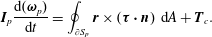 $$\begin{eqnarray}\displaystyle & \displaystyle \boldsymbol{I}_{p}\frac{\text{d}(\unicode[STIX]{x1D74E}_{p})}{\text{d}t}=\oint _{\unicode[STIX]{x2202}S_{p}}\boldsymbol{r}\times \left(\unicode[STIX]{x1D749}\boldsymbol{\cdot }\boldsymbol{n}\right)\,\text{d}A+\boldsymbol{T}_{c}. & \displaystyle\end{eqnarray}$$
Here
 $\boldsymbol{U}_{p}$
and
$\boldsymbol{U}_{p}$
and
 $\unicode[STIX]{x1D74E}_{p}$
are the translational and the angular velocity of the particle, and
$\unicode[STIX]{x1D74E}_{p}$
are the translational and the angular velocity of the particle, and
 $\unicode[STIX]{x1D70C}_{p}$
,
$\unicode[STIX]{x1D70C}_{p}$
,
 $V_{p}$
and
$V_{p}$
and
 $\boldsymbol{I}_{p}$
are the particle’s mass density, volume and moment of inertia. The outward unit normal vector at the particle surface is denoted by
$\boldsymbol{I}_{p}$
are the particle’s mass density, volume and moment of inertia. The outward unit normal vector at the particle surface is denoted by
 $\boldsymbol{n}$
, and
$\boldsymbol{n}$
, and
 $\boldsymbol{r}$
is the position vector from the particle’s centre. The integrated stress tensor
$\boldsymbol{r}$
is the position vector from the particle’s centre. The integrated stress tensor
 $\unicode[STIX]{x1D749}=-p\boldsymbol{I}+\unicode[STIX]{x1D707}_{f}(\unicode[STIX]{x1D735}\boldsymbol{u}+\unicode[STIX]{x1D735}\boldsymbol{u}^{\text{T}})$
on the surface of particles and the force terms
$\unicode[STIX]{x1D749}=-p\boldsymbol{I}+\unicode[STIX]{x1D707}_{f}(\unicode[STIX]{x1D735}\boldsymbol{u}+\unicode[STIX]{x1D735}\boldsymbol{u}^{\text{T}})$
on the surface of particles and the force terms
 $-\unicode[STIX]{x1D70C}_{f}V_{p}\boldsymbol{g}$
,
$-\unicode[STIX]{x1D70C}_{f}V_{p}\boldsymbol{g}$
,
 $V_{p}\unicode[STIX]{x1D735}p_{e}$
and
$V_{p}\unicode[STIX]{x1D735}p_{e}$
and
 $\boldsymbol{g}$
account for the fluid–solid interactions, the hydrostatic pressure, any external constant pressure gradient and the gravitational acceleration, respectively. Finally,
$\boldsymbol{g}$
account for the fluid–solid interactions, the hydrostatic pressure, any external constant pressure gradient and the gravitational acceleration, respectively. Finally,
 $\boldsymbol{F}_{c}$
and
$\boldsymbol{F}_{c}$
and
 $\boldsymbol{T}_{c}$
are the force and the torque, acting on the particles, due to the particle–particle (particle–wall) collisions.
$\boldsymbol{T}_{c}$
are the force and the torque, acting on the particles, due to the particle–particle (particle–wall) collisions.
The energy equation for incompressible flows can be simplified to
 $$\begin{eqnarray}\displaystyle \unicode[STIX]{x1D70C}C_{p}\left[\frac{\unicode[STIX]{x2202}T}{\unicode[STIX]{x2202}t}+\boldsymbol{u}\boldsymbol{\cdot }\unicode[STIX]{x1D735}T\right]=\unicode[STIX]{x1D735}\boldsymbol{\cdot }(k\unicode[STIX]{x1D735}T), & & \displaystyle\end{eqnarray}$$
where
 $C_{p}$
and
$C_{p}$
and
 $k$
are the specific heat capacity and thermal conductivity, and
$k$
are the specific heat capacity and thermal conductivity, and
 $T$
the temperature. Considering the same
$T$
the temperature. Considering the same
 $\unicode[STIX]{x1D70C}C_{p}$
for the fluid and particles (i.e.
$\unicode[STIX]{x1D70C}C_{p}$
for the fluid and particles (i.e.
 $(\unicode[STIX]{x1D70C}C_{p})_{p}=(\unicode[STIX]{x1D70C}C_{p})_{f}$
), as in this study, equation (2.5) reduces to
$(\unicode[STIX]{x1D70C}C_{p})_{p}=(\unicode[STIX]{x1D70C}C_{p})_{f}$
), as in this study, equation (2.5) reduces to
 $$\begin{eqnarray}\displaystyle \frac{\unicode[STIX]{x2202}T}{\unicode[STIX]{x2202}t}+\boldsymbol{u}\boldsymbol{\cdot }\unicode[STIX]{x1D735}T=\unicode[STIX]{x1D735}\boldsymbol{\cdot }(\unicode[STIX]{x1D6FC}\unicode[STIX]{x1D735}T), & & \displaystyle\end{eqnarray}$$
where
 $\unicode[STIX]{x1D6FC}$
is the thermal diffusivity, equal to
$\unicode[STIX]{x1D6FC}$
is the thermal diffusivity, equal to
 $k/(\unicode[STIX]{x1D70C}C_{p})$
.
$k/(\unicode[STIX]{x1D70C}C_{p})$
.
Equation (2.6) is resolved on every grid point in the computational domain, i.e. in the fluid and solid phases, with different thermal diffusivities:
 $\unicode[STIX]{x1D6FC}_{f}$
for the fluid phase and
$\unicode[STIX]{x1D6FC}_{f}$
for the fluid phase and
 $\unicode[STIX]{x1D6FC}_{p}$
for the particles.
$\unicode[STIX]{x1D6FC}_{p}$
for the particles.
2.2 Numerical scheme
Uhlmann (Reference Uhlmann2005) developed a computationally efficient IBM to fully resolve particle-laden flows. Breugem (Reference Breugem2012) introduced improvements to this method, making it second-order-accurate in space while increasing the numerical stability of the method for mass density ratios (particle over fluid density ratio) near unity (see also Kempe & Fröhlich Reference Kempe and Fröhlich2012). The IBM is coupled here with a VoF approach (Hirt & Nichols Reference Hirt and Nichols1981) to study the heat transfer in a suspension of rigid particles. The VoF approach has been suggested among others by Ström & Sasic (Reference Ström and Sasic2013) for resolving both heat and momentum transfer in the presence of solid particles.
Details on the IBM accounting for fluid–solid interactions are discussed in Breugem (Reference Breugem2012) and several validations can be found elsewhere (Lambert et al. Reference Lambert, Picano, Breugem and Brandt2013; Picano et al. Reference Picano, Breugem and Brandt2015; Ardekani et al. Reference Ardekani, Costa, Breugem and Brandt2016; Lashgari et al. Reference Lashgari, Picano, Breugem and Brandt2016). For clarity a short description of the IBM is given in the first two sections below, followed by the VoF method for heat transfer within the suspension.
2.2.1 Solution of the flow field
The flow field is resolved on a uniform (
 $\unicode[STIX]{x0394}x=\unicode[STIX]{x0394}y=\unicode[STIX]{x0394}z$
), staggered, Cartesian grid, while particles are represented by a set of Lagrangian points, uniformly distributed on the surface of each particle. The number of Lagrangian grid points
$\unicode[STIX]{x0394}x=\unicode[STIX]{x0394}y=\unicode[STIX]{x0394}z$
), staggered, Cartesian grid, while particles are represented by a set of Lagrangian points, uniformly distributed on the surface of each particle. The number of Lagrangian grid points
 $N_{L}$
on the surface of each particle is defined such that the Lagrangian grid volume
$N_{L}$
on the surface of each particle is defined such that the Lagrangian grid volume
 $\unicode[STIX]{x0394}V_{l}$
becomes equal to the volume of the Eulerian mesh
$\unicode[STIX]{x0394}V_{l}$
becomes equal to the volume of the Eulerian mesh
 $\unicode[STIX]{x0394}x^{3}$
. Thus
$\unicode[STIX]{x0394}x^{3}$
. Thus
 $\unicode[STIX]{x0394}V_{l}$
is obtained by assuming the particle to be a thin shell with the same thickness as the Eulerian grid size. A first prediction velocity is obtained by advancing (2.1) in time without considering the force field
$\unicode[STIX]{x0394}V_{l}$
is obtained by assuming the particle to be a thin shell with the same thickness as the Eulerian grid size. A first prediction velocity is obtained by advancing (2.1) in time without considering the force field
 $\boldsymbol{f}$
and neglecting the pressure-correction term (see Breugem (Reference Breugem2012) for the details of the pressure-correction scheme), using an explicit low-storage Runge–Kutta method. The first prediction velocity is then interpolated from the Eulerian grid to each Lagrangian point on the surface of the particle,
$\boldsymbol{f}$
and neglecting the pressure-correction term (see Breugem (Reference Breugem2012) for the details of the pressure-correction scheme), using an explicit low-storage Runge–Kutta method. The first prediction velocity is then interpolated from the Eulerian grid to each Lagrangian point on the surface of the particle,
 $\boldsymbol{U}_{l}^{\ast }$
(2.7), using the regularized Dirac delta function
$\boldsymbol{U}_{l}^{\ast }$
(2.7), using the regularized Dirac delta function
 $\unicode[STIX]{x1D6FF}_{d}$
of Roma, Peskin & Berger (Reference Roma, Peskin and Berger1999). The IBM point force
$\unicode[STIX]{x1D6FF}_{d}$
of Roma, Peskin & Berger (Reference Roma, Peskin and Berger1999). The IBM point force
 $F_{l}$
is then calculated at each Lagrangian point based on the difference between the particle surface velocity (
$F_{l}$
is then calculated at each Lagrangian point based on the difference between the particle surface velocity (
 $\boldsymbol{U}_{p}+\unicode[STIX]{x1D74E}_{p}\times \boldsymbol{r}$
) and the first interpolated prediction velocity (2.8). Lagrangian forces
$\boldsymbol{U}_{p}+\unicode[STIX]{x1D74E}_{p}\times \boldsymbol{r}$
) and the first interpolated prediction velocity (2.8). Lagrangian forces
 $F_{l}$
are interpolated back to the Eulerian grid by the same regularized Dirac delta function (see (2.9) below) and added to the first prediction velocity to obtain a second prediction velocity
$F_{l}$
are interpolated back to the Eulerian grid by the same regularized Dirac delta function (see (2.9) below) and added to the first prediction velocity to obtain a second prediction velocity
 $\boldsymbol{u}^{\ast \ast }$
(2.10). The second prediction velocity
$\boldsymbol{u}^{\ast \ast }$
(2.10). The second prediction velocity
 $\boldsymbol{u}^{\ast \ast }$
is then used to update velocities and pressure following a classic pressure-correction scheme. The calculation of
$\boldsymbol{u}^{\ast \ast }$
is then used to update velocities and pressure following a classic pressure-correction scheme. The calculation of
 $\boldsymbol{u}^{\ast \ast }$
is summarized below for a Runge–Kutta substep
$\boldsymbol{u}^{\ast \ast }$
is summarized below for a Runge–Kutta substep
 $q$
:
$q$
:
 $$\begin{eqnarray}\displaystyle & \displaystyle \boldsymbol{U}_{l}^{\ast }=\mathop{\sum }_{ijk}\boldsymbol{u}_{ijk}^{\ast }\unicode[STIX]{x1D6FF}_{d}(\boldsymbol{x}_{ijk}-\boldsymbol{X}_{l}^{q-1})\unicode[STIX]{x0394}x\unicode[STIX]{x0394}y\unicode[STIX]{x0394}z, & \displaystyle\end{eqnarray}$$
 $$\begin{eqnarray}\displaystyle & \displaystyle \boldsymbol{F}_{l}^{q-1/2}=\frac{\boldsymbol{U}(\boldsymbol{X}_{l}^{q-1})-\boldsymbol{U}_{l}^{\ast }}{\unicode[STIX]{x0394}t}, & \displaystyle\end{eqnarray}$$
 $$\begin{eqnarray}\displaystyle & \displaystyle \boldsymbol{f}_{ijk}^{q-1/2}=\mathop{\sum }_{l}\boldsymbol{F}_{l}^{q-1/2}\unicode[STIX]{x1D6FF}_{d}(\boldsymbol{x}_{ijk}-\boldsymbol{X}_{l}^{q-1})\unicode[STIX]{x0394}V_{l}, & \displaystyle\end{eqnarray}$$
 $$\begin{eqnarray}\displaystyle & \displaystyle \boldsymbol{u}^{\ast \ast }=\boldsymbol{u}^{\ast }+\unicode[STIX]{x0394}t\boldsymbol{f}^{q-1/2}, & \displaystyle\end{eqnarray}$$
where capital letters indicate the variable at a Lagrangian point with index
 $l$
and
$l$
and
 $\boldsymbol{x}_{ijk}$
refers to an Eulerian grid point.
$\boldsymbol{x}_{ijk}$
refers to an Eulerian grid point.
2.2.2 Solution of the particle motion
Taking into account the motion of rigid spherical particles and the mass of the fictitious fluid phase inside the particle volumes, Breugem (Reference Breugem2012) showed that (2.3) and (2.4) can be rewritten as
 $$\begin{eqnarray}\displaystyle & \displaystyle \unicode[STIX]{x1D70C}_{p}V_{p}\frac{\text{d}\boldsymbol{U}_{p}}{\text{d}t}\approx -\unicode[STIX]{x1D70C}_{f}\mathop{\sum }_{l=1}^{N_{L}}\boldsymbol{F}_{l}\unicode[STIX]{x0394}V_{l}+\unicode[STIX]{x1D70C}_{f}\frac{\text{d}}{\text{d}t}\left(\int _{V_{p}}\boldsymbol{u}\,\text{d}V\right)+(\unicode[STIX]{x1D70C}_{p}-\unicode[STIX]{x1D70C}_{f})V_{p}\boldsymbol{g}+\boldsymbol{F}_{c}, & \displaystyle\end{eqnarray}$$
 $$\begin{eqnarray}\displaystyle & \displaystyle \frac{\text{d}(\boldsymbol{I}_{p}\unicode[STIX]{x1D74E}_{p})}{\text{d}t}\approx -\unicode[STIX]{x1D70C}_{f}\mathop{\sum }_{l=1}^{N_{L}}\boldsymbol{r}_{l}\times \boldsymbol{F}_{l}\unicode[STIX]{x0394}V_{l}+\unicode[STIX]{x1D70C}_{f}\frac{\text{d}}{\text{d}t}\left(\int _{V_{p}}\boldsymbol{r}\times \boldsymbol{u}\,\text{d}V\right)+\boldsymbol{T}_{c}, & \displaystyle\end{eqnarray}$$
where the first term on the right-hand side of the equations is the IBM force and torque exerted on the particle. The second term directly accounts for the inertia of the fluid that is trapped inside the particles, when using IBM. The interaction force
 $\boldsymbol{F}_{c}$
and torque
$\boldsymbol{F}_{c}$
and torque
 $\boldsymbol{T}_{c}$
are activated when the gap width between the two particles (or between one particle and the wall) is less than one Eulerian grid size. Indeed, when the gap width reduces to less than one Eulerian mesh, the lubrication force is underpredicted by the IBM. To avoid computationally expensive grid refinements, a lubrication model based on the asymptotic analytical expression for the normal lubrication force between two equal spheres (Brenner Reference Brenner1961) is used here for particle–particle interactions, whereas the solution for two unequal spheres, one with infinite radius, is employed for particle–wall interactions. A soft-sphere collision model with Coulomb friction takes over the interaction when the particles touch. The restitution coefficients, used for normal and tangential collisions, are
$\boldsymbol{T}_{c}$
are activated when the gap width between the two particles (or between one particle and the wall) is less than one Eulerian grid size. Indeed, when the gap width reduces to less than one Eulerian mesh, the lubrication force is underpredicted by the IBM. To avoid computationally expensive grid refinements, a lubrication model based on the asymptotic analytical expression for the normal lubrication force between two equal spheres (Brenner Reference Brenner1961) is used here for particle–particle interactions, whereas the solution for two unequal spheres, one with infinite radius, is employed for particle–wall interactions. A soft-sphere collision model with Coulomb friction takes over the interaction when the particles touch. The restitution coefficients, used for normal and tangential collisions, are
 $0.97$
and
$0.97$
and
 $0.1$
, with Coulomb friction coefficient
$0.1$
, with Coulomb friction coefficient
 $0.15$
. More details about the short-range models and corresponding validations can be found in Costa et al. (Reference Costa, Boersma, Westerweel and Breugem2015) and Ardekani et al. (Reference Ardekani, Costa, Breugem and Brandt2016).
$0.15$
. More details about the short-range models and corresponding validations can be found in Costa et al. (Reference Costa, Boersma, Westerweel and Breugem2015) and Ardekani et al. (Reference Ardekani, Costa, Breugem and Brandt2016).
The equations above are integrated in time using the same explicit low-storage Runge–Kutta method used for the flow.
2.2.3 Solution of the temperature field
A phase indicator,
 $\unicode[STIX]{x1D709}$
, is used to distinguish the solid and the fluid phases within the computational domain. The
$\unicode[STIX]{x1D709}$
, is used to distinguish the solid and the fluid phases within the computational domain. The
 $\unicode[STIX]{x1D709}$
value is computed at the velocity (cell faces) and the pressure points (cell centre) throughout the staggered Eulerian grid. This value varies between
$\unicode[STIX]{x1D709}$
value is computed at the velocity (cell faces) and the pressure points (cell centre) throughout the staggered Eulerian grid. This value varies between
 $0$
and
$0$
and
 $1$
based on the solid volume fraction of a cell of size
$1$
based on the solid volume fraction of a cell of size
 $\unicode[STIX]{x0394}x$
around the desired point. As we know the exact location of the fluid–solid interface for rigid spheres, a level-set function
$\unicode[STIX]{x0394}x$
around the desired point. As we know the exact location of the fluid–solid interface for rigid spheres, a level-set function
 $\unicode[STIX]{x1D701}$
given by the signed distance to the particle surface
$\unicode[STIX]{x1D701}$
given by the signed distance to the particle surface
 ${\mathcal{S}}$
is employed to determine
${\mathcal{S}}$
is employed to determine
 $\unicode[STIX]{x1D709}$
at each point. With
$\unicode[STIX]{x1D709}$
at each point. With
 $\unicode[STIX]{x1D701}<0$
inside and
$\unicode[STIX]{x1D701}<0$
inside and
 $\unicode[STIX]{x1D701}>0$
outside the particle, the solid volume fraction is calculated similar to Kempe & Fröhlich (Reference Kempe and Fröhlich2012):
$\unicode[STIX]{x1D701}>0$
outside the particle, the solid volume fraction is calculated similar to Kempe & Fröhlich (Reference Kempe and Fröhlich2012):
 $$\begin{eqnarray}\displaystyle \unicode[STIX]{x1D709}=\frac{\mathop{\sum }_{n=1}^{8}-\unicode[STIX]{x1D701}_{n}{\mathcal{H}}(-\unicode[STIX]{x1D701}_{n})}{\mathop{\sum }_{n=1}^{8}|\unicode[STIX]{x1D701}_{n}|}, & & \displaystyle\end{eqnarray}$$
where the sum is over all eight corners of a box of size
 $\unicode[STIX]{x0394}x$
around the target point and
$\unicode[STIX]{x0394}x$
around the target point and
 ${\mathcal{H}}$
is the Heaviside step function. Figure 1 indicates the staggered Eulerian grid and the phase indicator
${\mathcal{H}}$
is the Heaviside step function. Figure 1 indicates the staggered Eulerian grid and the phase indicator
 $\unicode[STIX]{x1D709}$
around the velocity point
$\unicode[STIX]{x1D709}$
around the velocity point
 $u_{i-1/2,j}$
.
$u_{i-1/2,j}$
.
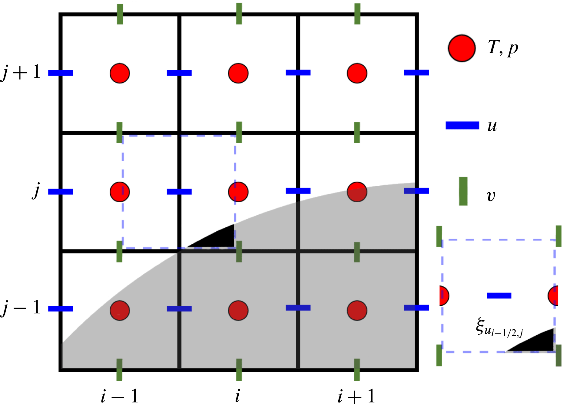
Figure 1. The staggered Eulerian grid and the phase indicator
 $\unicode[STIX]{x1D709}$
around the velocity point
$\unicode[STIX]{x1D709}$
around the velocity point
 $u_{i-1/2,j}$
.
$u_{i-1/2,j}$
.
Using a VoF approach (Hirt & Nichols Reference Hirt and Nichols1981), the velocity and the thermal diffusivity of the combined phase are defined at each point in the domain as
 $$\begin{eqnarray}\displaystyle & \displaystyle \boldsymbol{u}_{cp}=(1-\unicode[STIX]{x1D709})\boldsymbol{u}_{f}+\unicode[STIX]{x1D709}\boldsymbol{u}_{p}, & \displaystyle\end{eqnarray}$$
 $$\begin{eqnarray}\displaystyle & \displaystyle \unicode[STIX]{x1D6FC}_{cp}=(1-\unicode[STIX]{x1D709})\unicode[STIX]{x1D6FC}_{f}+\unicode[STIX]{x1D709}\unicode[STIX]{x1D6FC}_{p}, & \displaystyle\end{eqnarray}$$
where
 $\boldsymbol{u}_{f}$
is the fluid velocity and
$\boldsymbol{u}_{f}$
is the fluid velocity and
 $\boldsymbol{u}_{p}$
the solid-phase velocity, obtained by the rigid-body motion of the particle at the desired point;
$\boldsymbol{u}_{p}$
the solid-phase velocity, obtained by the rigid-body motion of the particle at the desired point;
 $\unicode[STIX]{x1D6FC}_{f}$
and
$\unicode[STIX]{x1D6FC}_{f}$
and
 $\unicode[STIX]{x1D6FC}_{p}$
denote the thermal diffusivity of the fluid and the solid phase.
$\unicode[STIX]{x1D6FC}_{p}$
denote the thermal diffusivity of the fluid and the solid phase.
Substituting
 $\boldsymbol{u}_{cp}$
and
$\boldsymbol{u}_{cp}$
and
 $\unicode[STIX]{x1D6FC}_{cp}$
in (2.6) and taking into account that the velocity field
$\unicode[STIX]{x1D6FC}_{cp}$
in (2.6) and taking into account that the velocity field
 $\boldsymbol{u}_{cp}$
is divergence-free results in
$\boldsymbol{u}_{cp}$
is divergence-free results in
 $$\begin{eqnarray}\displaystyle \frac{\unicode[STIX]{x2202}T}{\unicode[STIX]{x2202}t}+\unicode[STIX]{x1D735}\boldsymbol{\cdot }(\boldsymbol{u}_{cp}T)=\unicode[STIX]{x1D735}\boldsymbol{\cdot }(\unicode[STIX]{x1D6FC}_{cp}\unicode[STIX]{x1D735}T), & & \displaystyle\end{eqnarray}$$
which is discretized around the Eulerian cell centres (pressure and temperature points on the Eulerian staggered grid) and integrated in time, using the same explicit low-storage Runge–Kutta method used for marching the flow and particle equations.
2.3 Flow configuration
In the present work, the Couette flow between two infinite walls a distance
 $2h$
apart in the wall-normal direction,
$2h$
apart in the wall-normal direction,
 $y$
, is investigated. The size of the computational domain is
$y$
, is investigated. The size of the computational domain is
 $L_{x}=4h$
,
$L_{x}=4h$
,
 $L_{y}=2h$
and
$L_{y}=2h$
and
 $L_{z}=2h$
in the streamwise, wall-normal and spanwise directions. Periodic boundary conditions for velocity, temperature and particles are imposed in both streamwise and spanwise directions (
$L_{z}=2h$
in the streamwise, wall-normal and spanwise directions. Periodic boundary conditions for velocity, temperature and particles are imposed in both streamwise and spanwise directions (
 $x$
and
$x$
and
 $z$
), while the upper and lower walls are moving with velocity
$z$
), while the upper and lower walls are moving with velocity
 $0.5U_{b}$
and
$0.5U_{b}$
and
 $-0.5U_{b}$
. Here
$-0.5U_{b}$
. Here
 $U_{b}$
is the reference velocity, used to define the flow Reynolds number
$U_{b}$
is the reference velocity, used to define the flow Reynolds number
 $Re_{b}=U_{b}2h/\unicode[STIX]{x1D708}$
, with
$Re_{b}=U_{b}2h/\unicode[STIX]{x1D708}$
, with
 $\unicode[STIX]{x1D708}$
the kinematic viscosity of the fluid phase. The diameter of the particles considered in this study is equal to one-sixth of the distance between the planes (
$\unicode[STIX]{x1D708}$
the kinematic viscosity of the fluid phase. The diameter of the particles considered in this study is equal to one-sixth of the distance between the planes (
 $2h/D=6$
) and the particle Reynolds number is defined as
$2h/D=6$
) and the particle Reynolds number is defined as
 $Re_{p}=\dot{\unicode[STIX]{x1D6FE}}D^{2}/\unicode[STIX]{x1D708}$
, where
$Re_{p}=\dot{\unicode[STIX]{x1D6FE}}D^{2}/\unicode[STIX]{x1D708}$
, where
 $\dot{\unicode[STIX]{x1D6FE}}=U_{b}/2h$
is the shear rate. The temperature is non-dimensionalized by
$\dot{\unicode[STIX]{x1D6FE}}=U_{b}/2h$
is the shear rate. The temperature is non-dimensionalized by
 $(T-T_{avg})/(T_{hot}-T_{cold})$
, where
$(T-T_{avg})/(T_{hot}-T_{cold})$
, where
 $T_{hot}$
and
$T_{hot}$
and
 $T_{cold}$
are the operating temperatures at the walls and
$T_{cold}$
are the operating temperatures at the walls and
 $T_{avg}$
is their average. Therefore, the non-dimensional temperatures
$T_{avg}$
is their average. Therefore, the non-dimensional temperatures
 $T$
for the upper and lower walls are fixed at
$T$
for the upper and lower walls are fixed at
 $T=-0.5$
and
$T=-0.5$
and
 $0.5$
.
$0.5$
.
Simulations are performed at different particle Reynolds number
 $Re_{p}$
, volume fraction
$Re_{p}$
, volume fraction
 $\unicode[STIX]{x1D719}$
(total volume of the particles over the volume of the computational domain) and thermal diffusivity ratio
$\unicode[STIX]{x1D719}$
(total volume of the particles over the volume of the computational domain) and thermal diffusivity ratio
 $\unicode[STIX]{x1D6E4}\equiv \unicode[STIX]{x1D6FC}_{p}/\unicode[STIX]{x1D6FC}_{f}$
. We investigate the effect of each parameter on the heat transfer between the two walls and quantify the results in terms of
$\unicode[STIX]{x1D6E4}\equiv \unicode[STIX]{x1D6FC}_{p}/\unicode[STIX]{x1D6FC}_{f}$
. We investigate the effect of each parameter on the heat transfer between the two walls and quantify the results in terms of
 $\unicode[STIX]{x1D6FC}_{r}\equiv \unicode[STIX]{x1D6FC}_{e}/\unicode[STIX]{x1D6FC}_{f}$
, with
$\unicode[STIX]{x1D6FC}_{r}\equiv \unicode[STIX]{x1D6FC}_{e}/\unicode[STIX]{x1D6FC}_{f}$
, with
 $\unicode[STIX]{x1D6FC}_{e}$
denoting the effective thermal diffusivity of the suspension. This is the diffusivity that would correspond to the heat flux extracted from the numerical data,
$\unicode[STIX]{x1D6FC}_{e}$
denoting the effective thermal diffusivity of the suspension. This is the diffusivity that would correspond to the heat flux extracted from the numerical data,
 $q^{\prime \prime }$
, with the temperature gradient of the single-phase flow:
$q^{\prime \prime }$
, with the temperature gradient of the single-phase flow:
 $$\begin{eqnarray}\displaystyle \left.\unicode[STIX]{x1D6FC}_{e}=q^{\prime \prime }\!/\frac{\text{d}T}{\text{d}y}\right|_{\unicode[STIX]{x1D719}=0\,\%}. & & \displaystyle\end{eqnarray}$$
The different parameters investigated are reported in table 1. Simulations are performed with an Eulerian grid of
 $24$
grid points per diameter of the spherical particles, corresponding to
$24$
grid points per diameter of the spherical particles, corresponding to
 $288\times 144\times 144$
Eulerian grid points over the computational domain, with
$288\times 144\times 144$
Eulerian grid points over the computational domain, with
 $1721$
Lagrangian points used to represent the surface of each particle.
$1721$
Lagrangian points used to represent the surface of each particle.
To check if the grid resolution is adequate to carry out the simulations, two cases (
 $Re_{p}=16$
,
$Re_{p}=16$
,
 $\unicode[STIX]{x1D6E4}=1$
at
$\unicode[STIX]{x1D6E4}=1$
at
 $\unicode[STIX]{x1D719}=10\,\%$
and
$\unicode[STIX]{x1D719}=10\,\%$
and
 $20\,\%$
) are re-simulated with resolutions of
$20\,\%$
) are re-simulated with resolutions of
 $32$
and
$32$
and
 $40$
grid points per particle diameter. The effective thermal diffusivities obtained from these high-resolution cases are depicted in figure 2, where the results are normalized by the value of
$40$
grid points per particle diameter. The effective thermal diffusivities obtained from these high-resolution cases are depicted in figure 2, where the results are normalized by the value of
 $\unicode[STIX]{x1D6FC}_{r}$
for the resolution of
$\unicode[STIX]{x1D6FC}_{r}$
for the resolution of
 $24$
. It can be observed that the difference is less than
$24$
. It can be observed that the difference is less than
 $3.8\,\%$
when increasing the resolution to
$3.8\,\%$
when increasing the resolution to
 $40$
grid points per particle diameter; therefore, we choose the resolution of
$40$
grid points per particle diameter; therefore, we choose the resolution of
 $24$
to be able to perform the parameter study presented here with numerous simulations.
$24$
to be able to perform the parameter study presented here with numerous simulations.
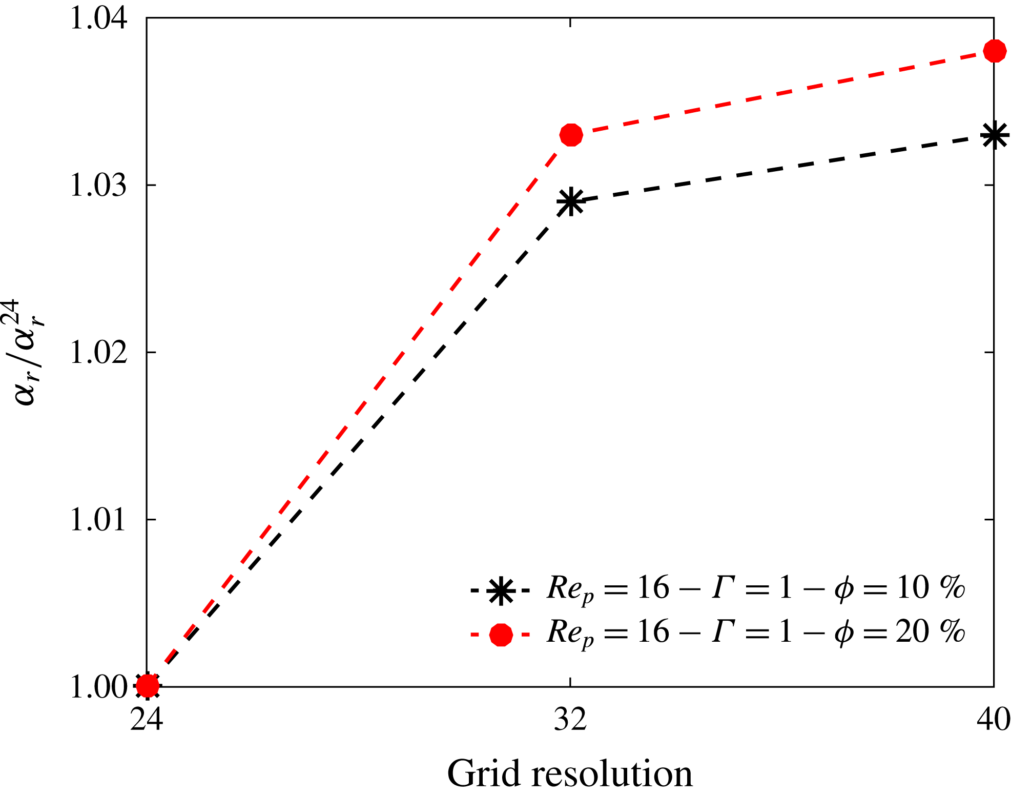
Figure 2. The effective thermal diffusivities, normalized by the value of
 $\unicode[STIX]{x1D6FC}_{r}$
for
$\unicode[STIX]{x1D6FC}_{r}$
for
 $24$
grid points per particle diameter (
$24$
grid points per particle diameter (
 $\unicode[STIX]{x1D6FC}_{r}^{24}$
), versus grid resolution per particle diameter.
$\unicode[STIX]{x1D6FC}_{r}^{24}$
), versus grid resolution per particle diameter.
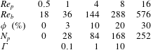
Table 1. Summary of the different parameters under investigation. From the top: particle Reynolds number
 $Re_{p}$
and the corresponding bulk Reynolds number
$Re_{p}$
and the corresponding bulk Reynolds number
 $Re_{b}$
; suspension volume fraction
$Re_{b}$
; suspension volume fraction
 $\unicode[STIX]{x1D719}$
and corresponding number of particles
$\unicode[STIX]{x1D719}$
and corresponding number of particles
 $N_{p}$
inside the computational domain; and ratio between the thermal diffusivity of the particles and of the fluid,
$N_{p}$
inside the computational domain; and ratio between the thermal diffusivity of the particles and of the fluid,
 $\unicode[STIX]{x1D6E4}$
.
$\unicode[STIX]{x1D6E4}$
.
The simulations are started with a random distribution of particles inside the domain and a linear temperature field between
 $-0.5$
and
$-0.5$
and
 $0.5$
for both the fluid and the particles. Statistics are collected over an interval of almost
$0.5$
for both the fluid and the particles. Statistics are collected over an interval of almost
 $10\,000$
in units of
$10\,000$
in units of
 $D/U_{b}$
after the wall-normal heat flux has reached a steady-state value with small oscillations in time. The statistics presented are averages in time and wall-parallel directions.
$D/U_{b}$
after the wall-normal heat flux has reached a steady-state value with small oscillations in time. The statistics presented are averages in time and wall-parallel directions.
3 Validation
The IBM used in this study to resolve the fluid–solid interaction has been fully validated by Breugem (Reference Breugem2012) and Picano et al. (Reference Picano, Breugem, Mitra and Brandt2013, Reference Picano, Breugem and Brandt2015). The validation of the temperature solver with the mentioned VoF approach for the heat transfer between the phases is presented here, considering first a single sphere.

Figure 3. (a) A two-dimensional section of the boundary-fitted orthogonal grid used in the finite volume solver. (b) Effective thermal diffusivity
 $\unicode[STIX]{x1D6FC}_{e}$
normalized by the thermal diffusivity of the fluid (
$\unicode[STIX]{x1D6FC}_{e}$
normalized by the thermal diffusivity of the fluid (
 $\unicode[STIX]{x1D6FC}_{r}\equiv \unicode[STIX]{x1D6FC}_{e}/\unicode[STIX]{x1D6FC}_{f}$
) for different thermal diffusivity ratios
$\unicode[STIX]{x1D6FC}_{r}\equiv \unicode[STIX]{x1D6FC}_{e}/\unicode[STIX]{x1D6FC}_{f}$
) for different thermal diffusivity ratios
 $\unicode[STIX]{x1D6E4}$
between the particle and the fluid.
$\unicode[STIX]{x1D6E4}$
between the particle and the fluid.
The numerical code developed for this study enjoys the ability to resolve the temperature field across the domain with different thermal diffusivities for the particles and the fluid. When there is a significant difference between the thermal diffusivities of the solid and the fluid, the coefficient in the diffusion term of the temperature equation experiences a jump across the interface. This jump is smoothed around the interface in the present numerical scheme. To evaluate how the present numerical model performs for these situations, a simpler validation case is chosen.
We consider a computational domain of size
 $3D\times 3D\times 3D$
with a sphere in the centre and vary the ratio of the thermal diffusivities of the sphere and of the surrounding fluid,
$3D\times 3D\times 3D$
with a sphere in the centre and vary the ratio of the thermal diffusivities of the sphere and of the surrounding fluid,
 $\unicode[STIX]{x1D6E4}$
. The non-dimensional temperatures at the upper and lower walls of the domain are set to
$\unicode[STIX]{x1D6E4}$
. The non-dimensional temperatures at the upper and lower walls of the domain are set to
 $T=-0.5$
and
$T=-0.5$
and
 $0.5$
, respectively, while periodic boundary conditions are imposed on the other four faces of the cube. The fluid and the particle are at rest and we thus solve only the temperature equation, in particular, the diffusive terms. This case is simulated with the present numerical code over a uniform Cartesian grid with a resolution of
$0.5$
, respectively, while periodic boundary conditions are imposed on the other four faces of the cube. The fluid and the particle are at rest and we thus solve only the temperature equation, in particular, the diffusive terms. This case is simulated with the present numerical code over a uniform Cartesian grid with a resolution of
 $24$
grid points per diameter of the sphere. The results of this simulation are compared with a finite volume solver (ANSYS Fluent commercial software), using an orthogonal body-fitted grid around the sphere and the box surfaces, in which the body-fitted mesh allows the solver to capture the sharp temperature gradients at the interface accurately. Figure 3(a) shows a two-dimensional section of the grid across the middle of the computational domain. In the commercial solver the diffusion terms of the temperature equation are discretized by a central difference scheme and an implicit solver for the discretized equation. The same case is simulated with
$24$
grid points per diameter of the sphere. The results of this simulation are compared with a finite volume solver (ANSYS Fluent commercial software), using an orthogonal body-fitted grid around the sphere and the box surfaces, in which the body-fitted mesh allows the solver to capture the sharp temperature gradients at the interface accurately. Figure 3(a) shows a two-dimensional section of the grid across the middle of the computational domain. In the commercial solver the diffusion terms of the temperature equation are discretized by a central difference scheme and an implicit solver for the discretized equation. The same case is simulated with
 $100\,000$
and
$100\,000$
and
 $360\,000$
grid cells to ensure grid convergence. The temperature field reaches a steady-state solution in time, given the constant temperatures at the walls. We report the effective thermal diffusivity, computed based on (2.17), normalized by the thermal diffusivity of the fluid phase in figure 3(b) for both the present numerical code and the finite volume solver over the boundary-fitted grid. It is observed that the results perfectly match each other for the range of thermal diffusivity ratios
$360\,000$
grid cells to ensure grid convergence. The temperature field reaches a steady-state solution in time, given the constant temperatures at the walls. We report the effective thermal diffusivity, computed based on (2.17), normalized by the thermal diffusivity of the fluid phase in figure 3(b) for both the present numerical code and the finite volume solver over the boundary-fitted grid. It is observed that the results perfectly match each other for the range of thermal diffusivity ratios
 $\unicode[STIX]{x1D6E4}$
investigated in this study.
$\unicode[STIX]{x1D6E4}$
investigated in this study.

Figure 4. Effective thermal diffusivity, normalized by the thermal diffusivity of the single-phase flow,
 $\unicode[STIX]{x1D6FC}_{r}$
, for the different volume fractions under investigation. The parameters for these simulations are set to
$\unicode[STIX]{x1D6FC}_{r}$
, for the different volume fractions under investigation. The parameters for these simulations are set to
 $Pr=20$
,
$Pr=20$
,
 $2h/D=6$
,
$2h/D=6$
,
 $Re_{p}=0.5$
and
$Re_{p}=0.5$
and
 $Pe=Re_{p}Pr=10$
.
$Pe=Re_{p}Pr=10$
.
As further validation, directly relevant to this work, we recall that Metzger et al. (Reference Metzger, Rahli and Yin2013) have proposed a correlation (
 $\unicode[STIX]{x1D6FC}_{e}/\unicode[STIX]{x1D6FC}_{f}=1+0.046\unicode[STIX]{x1D719}Pe$
) based on experimental and numerical data of spherical particles in a Couette flow in the inertialess Stokes regime, i.e. valid when the particle Reynolds number is less than
$\unicode[STIX]{x1D6FC}_{e}/\unicode[STIX]{x1D6FC}_{f}=1+0.046\unicode[STIX]{x1D719}Pe$
) based on experimental and numerical data of spherical particles in a Couette flow in the inertialess Stokes regime, i.e. valid when the particle Reynolds number is less than
 $0.5$
. As validation of our numerical code, simulations are therefore performed at
$0.5$
. As validation of our numerical code, simulations are therefore performed at
 $Re_{p}=0.5$
for different volume fractions
$Re_{p}=0.5$
for different volume fractions
 $10,~20$
and
$10,~20$
and
 $30\,\%$
with
$30\,\%$
with
 $\unicode[STIX]{x1D6E4}=1$
. The Prandtl number is set to
$\unicode[STIX]{x1D6E4}=1$
. The Prandtl number is set to
 $20$
and the results compared to the correlation in Metzger et al. (Reference Metzger, Rahli and Yin2013). Figure 4 depicts the comparison between the effective thermal diffusivity of the suspension, normalized by the thermal diffusivity of the single-phase flow,
$20$
and the results compared to the correlation in Metzger et al. (Reference Metzger, Rahli and Yin2013). Figure 4 depicts the comparison between the effective thermal diffusivity of the suspension, normalized by the thermal diffusivity of the single-phase flow,
 $\unicode[STIX]{x1D6FC}_{r}$
, obtained in this work and the suggested correlation. It is observed that the present numerical results are in good agreement with the empirical fit in the literature, as further shown when discussing the results.
$\unicode[STIX]{x1D6FC}_{r}$
, obtained in this work and the suggested correlation. It is observed that the present numerical results are in good agreement with the empirical fit in the literature, as further shown when discussing the results.
4 Heat transfer in a particle suspension subject to uniform shear
4.1 Effect of the particle inertia on the heat transfer

Figure 5. Snapshots of the temperature in the suspension flow for the volume fractions
 $\unicode[STIX]{x1D719}=10,~20$
and
$\unicode[STIX]{x1D719}=10,~20$
and
 $30\,\%$
at
$30\,\%$
at
 $Re_{p}=16$
.
$Re_{p}=16$
.
Having shown that the current implementation can reproduce the correlations obtained experimentally and numerically in the limit of vanishing inertia, when particle Reynolds number is sufficiently small
 $Re_{p}\leqslant 0.5$
(Metzger et al.
Reference Metzger, Rahli and Yin2013), we shall focus first on the effect of Reynolds number, finite inertia, on the heat transfer. We will consider dilute and semi-dilute suspensions at volume fractions
$Re_{p}\leqslant 0.5$
(Metzger et al.
Reference Metzger, Rahli and Yin2013), we shall focus first on the effect of Reynolds number, finite inertia, on the heat transfer. We will consider dilute and semi-dilute suspensions at volume fractions
 $\unicode[STIX]{x1D719}=3,~10,~20$
and
$\unicode[STIX]{x1D719}=3,~10,~20$
and
 $30\,\%$
with Prandtl number
$30\,\%$
with Prandtl number
 $Pr=7$
and particles of the same diffusivity as the fluid (
$Pr=7$
and particles of the same diffusivity as the fluid (
 $\unicode[STIX]{x1D6E4}=\unicode[STIX]{x1D6FC}_{p}/\unicode[STIX]{x1D6FC}_{f}=1$
). The simulations are performed with four values of the particle Reynolds number,
$\unicode[STIX]{x1D6E4}=\unicode[STIX]{x1D6FC}_{p}/\unicode[STIX]{x1D6FC}_{f}=1$
). The simulations are performed with four values of the particle Reynolds number,
 $Re_{p}=1,~4,~8$
and
$Re_{p}=1,~4,~8$
and
 $16$
.
$16$
.
Snapshots of the temperature in the suspension flow are shown in figure 5 for the volume fractions
 $\unicode[STIX]{x1D719}=10,~20$
and
$\unicode[STIX]{x1D719}=10,~20$
and
 $30\,\%$
at
$30\,\%$
at
 $Re_{p}=16$
. The instantaneous temperature is represented on different orthogonal planes with the bottom plane located near the bottom wall. Finite-size particles are displayed only on one half of the domain to give a visual feeling on how dense the solid phase is. The layering of the particles and movement between the layers can be observed for
$Re_{p}=16$
. The instantaneous temperature is represented on different orthogonal planes with the bottom plane located near the bottom wall. Finite-size particles are displayed only on one half of the domain to give a visual feeling on how dense the solid phase is. The layering of the particles and movement between the layers can be observed for
 $\unicode[STIX]{x1D719}=30\,\%$
. There is a noisy pattern in the temperature distribution due to the particles motion and fluctuations. At higher volume fractions these noisy patterns are stronger and more observable, as we will quantify in the following.
$\unicode[STIX]{x1D719}=30\,\%$
. There is a noisy pattern in the temperature distribution due to the particles motion and fluctuations. At higher volume fractions these noisy patterns are stronger and more observable, as we will quantify in the following.
Figure 6. The effective thermal diffusivity of the plain Couette flow, normalized with that for the single-phase flow,
 $\unicode[STIX]{x1D6FC}_{r}$
, versus (a) volume fraction percentage
$\unicode[STIX]{x1D6FC}_{r}$
, versus (a) volume fraction percentage
 $\unicode[STIX]{x1D719}$
, (b) particle Reynolds number
$\unicode[STIX]{x1D719}$
, (b) particle Reynolds number
 $Re_{p}$
and (c)
$Re_{p}$
and (c)
 $\unicode[STIX]{x1D719}Pe$
. The linear correlation, suggested by Metzger et al. (Reference Metzger, Rahli and Yin2013) is depicted in (a) and (c) by black dotted lines and the difference between this correlation and the DNS results are depicted in (d). The cases denoted as NR show the results of the simulations with non-rotating particles.
$\unicode[STIX]{x1D719}Pe$
. The linear correlation, suggested by Metzger et al. (Reference Metzger, Rahli and Yin2013) is depicted in (a) and (c) by black dotted lines and the difference between this correlation and the DNS results are depicted in (d). The cases denoted as NR show the results of the simulations with non-rotating particles.
The effective thermal diffusivity of the suspension, normalized with that of the single-phase flow,
 $\unicode[STIX]{x1D6FC}_{r}$
, is reported in figure 6(a) for all cases under investigation. The correlation suggested by Metzger et al. (Reference Metzger, Rahli and Yin2013) is also depicted. This correlation shows a linear variation of the effective thermal diffusivity of the suspension with the particle volume fraction in the Stokes regime. The data are observed to follow the relation proposed in Metzger et al. (Reference Metzger, Rahli and Yin2013) at the two lowest
$\unicode[STIX]{x1D6FC}_{r}$
, is reported in figure 6(a) for all cases under investigation. The correlation suggested by Metzger et al. (Reference Metzger, Rahli and Yin2013) is also depicted. This correlation shows a linear variation of the effective thermal diffusivity of the suspension with the particle volume fraction in the Stokes regime. The data are observed to follow the relation proposed in Metzger et al. (Reference Metzger, Rahli and Yin2013) at the two lowest
 $Re_{p}$
and then deviate as
$Re_{p}$
and then deviate as
 $Re_{p}$
increases. At high
$Re_{p}$
increases. At high
 $Re_{p}$
, the almost-linear profile of
$Re_{p}$
, the almost-linear profile of
 $\unicode[STIX]{x1D6FC}_{r}$
changes to a curve, which is underpredicted and overpredicted (by the mentioned correlation) for low and high volume fractions, respectively. Metzger et al. (Reference Metzger, Rahli and Yin2013) report a sudden decrease of the effective thermal diffusivity when the volume fraction exceeds
$\unicode[STIX]{x1D6FC}_{r}$
changes to a curve, which is underpredicted and overpredicted (by the mentioned correlation) for low and high volume fractions, respectively. Metzger et al. (Reference Metzger, Rahli and Yin2013) report a sudden decrease of the effective thermal diffusivity when the volume fraction exceeds
 $40\,\%$
, due to steric effects. This sudden decrease seems to be substituted by a smooth saturation of the effective thermal diffusivity at lower volume fractions in the inertial regimes (high
$40\,\%$
, due to steric effects. This sudden decrease seems to be substituted by a smooth saturation of the effective thermal diffusivity at lower volume fractions in the inertial regimes (high
 $Re_{p}$
).
$Re_{p}$
).
An attempt is made in this work to study the role of particle rotation on the heat and momentum transfer between the two walls. For this purpose, a set of additional simulations are performed at
 $Re_{p}=16$
with different volume fractions, while imposing zero particle angular velocity, i.e. the particles are free to move but they cannot rotate. The results of these simulations are depicted in figure 6(a), denoted as NR (non-rotating). The data show a significant increase in the heat transfer for volume fractions
$Re_{p}=16$
with different volume fractions, while imposing zero particle angular velocity, i.e. the particles are free to move but they cannot rotate. The results of these simulations are depicted in figure 6(a), denoted as NR (non-rotating). The data show a significant increase in the heat transfer for volume fractions
 $\unicode[STIX]{x1D719}=3,~10$
and
$\unicode[STIX]{x1D719}=3,~10$
and
 $20\,\%$
with respect to the reference cases (with rotation) at the same
$20\,\%$
with respect to the reference cases (with rotation) at the same
 $Re_{p}$
. At
$Re_{p}$
. At
 $\unicode[STIX]{x1D719}=30\,\%$
, however,
$\unicode[STIX]{x1D719}=30\,\%$
, however,
 $\unicode[STIX]{x1D6FC}_{r}$
is barely affected.
$\unicode[STIX]{x1D6FC}_{r}$
is barely affected.
Figure 6(b) depicts the same data as in figure 6(a), the normalized effective thermal diffusivity, now displayed versus
 $Re_{p}$
for the different volume fractions considered. The results show that the normalized effective diffusivity
$Re_{p}$
for the different volume fractions considered. The results show that the normalized effective diffusivity
 $\unicode[STIX]{x1D6FC}_{r}$
varies almost linearly with
$\unicode[STIX]{x1D6FC}_{r}$
varies almost linearly with
 $Re_{p}$
at fixed volume fraction in the range of
$Re_{p}$
at fixed volume fraction in the range of
 $Re_{p}$
studied here. It should be noted that the thermal diffusivity inside the particles is the same as that of the fluid for the results in this section, hence only the wall-normal particle motions can enhance the mean diffusion. Depicting the results versus
$Re_{p}$
studied here. It should be noted that the thermal diffusivity inside the particles is the same as that of the fluid for the results in this section, hence only the wall-normal particle motions can enhance the mean diffusion. Depicting the results versus
 $\unicode[STIX]{x1D719}Pe$
as in figure 6(c), where
$\unicode[STIX]{x1D719}Pe$
as in figure 6(c), where
 $Pe$
is the Péclet number defined as
$Pe$
is the Péclet number defined as
 $PrRe_{p}$
, demonstrates that the linear trend suggested by Metzger et al. (Reference Metzger, Rahli and Yin2013) for the Stokes regime can approximate well the effective thermal diffusivity up to roughly
$PrRe_{p}$
, demonstrates that the linear trend suggested by Metzger et al. (Reference Metzger, Rahli and Yin2013) for the Stokes regime can approximate well the effective thermal diffusivity up to roughly
 $Re_{p}=4$
. A difference between the DNS results and the correlation is depicted in figure 6(d), where it can be observed that the difference is less than
$Re_{p}=4$
. A difference between the DNS results and the correlation is depicted in figure 6(d), where it can be observed that the difference is less than
 $\pm 4\,\%$
up to
$\pm 4\,\%$
up to
 $Re_{p}=4$
.
$Re_{p}=4$
.
Figure 7. (a) Effective viscosity of the suspension normalized by the viscosity of the fluid and (b) the ratio between the increase of the heat transfer
 $\unicode[STIX]{x1D6FC}_{r}$
and the increase of the suspension effective viscosity
$\unicode[STIX]{x1D6FC}_{r}$
and the increase of the suspension effective viscosity
 $\unicode[STIX]{x1D708}_{r}$
.
$\unicode[STIX]{x1D708}_{r}$
.
One aspect that should be considered when aiming to increase the heat transfer by employing particulate flows is that the increase of the effective thermal diffusivity usually comes at the price of an increase in the effective viscosity of the flow. This means a higher friction at the walls and higher external power needed to drive the flow. To quantitatively address this issue, the effective viscosity of the suspension
 $\unicode[STIX]{x1D708}_{e}$
, normalized by the viscosity of the single-phase flow,
$\unicode[STIX]{x1D708}_{e}$
, normalized by the viscosity of the single-phase flow,
 $\unicode[STIX]{x1D708}_{r}\equiv \unicode[STIX]{x1D708}_{e}/\unicode[STIX]{x1D708}_{f}$
, is computed for all cases and depicted in figure 7(a) versus
$\unicode[STIX]{x1D708}_{r}\equiv \unicode[STIX]{x1D708}_{e}/\unicode[STIX]{x1D708}_{f}$
, is computed for all cases and depicted in figure 7(a) versus
 $Re_{p}$
. The data confirm an increase of the suspension viscosity with
$Re_{p}$
. The data confirm an increase of the suspension viscosity with
 $\unicode[STIX]{x1D719}$
and with fluid and particle inertia: the former, at low
$\unicode[STIX]{x1D719}$
and with fluid and particle inertia: the former, at low
 $Re_{p}$
, closely follows classical empirical fits, e.g. Eiler’s fit (Stickel & Powell Reference Stickel and Powell2005), whereas the latter, also denoted as inertial shear thickening, is discussed and explained in Picano et al. (Reference Picano, Breugem, Mitra and Brandt2013), among others.
$Re_{p}$
, closely follows classical empirical fits, e.g. Eiler’s fit (Stickel & Powell Reference Stickel and Powell2005), whereas the latter, also denoted as inertial shear thickening, is discussed and explained in Picano et al. (Reference Picano, Breugem, Mitra and Brandt2013), among others.
The ratio between
 $\unicode[STIX]{x1D6FC}_{r}$
and
$\unicode[STIX]{x1D6FC}_{r}$
and
 $\unicode[STIX]{x1D708}_{r}$
can be used to measure the global efficiency of the heat transfer increase, taking into account the external power needed to drive the flow: a value of this ratio larger than 1 means that the presence of particles increases heat transfer more than the momentum transfer, while for a ratio smaller than 1 the opposite is true. This ratio can be interpreted as an effective Prandtl number of the suspension, similarly to the turbulent Prandtl number used to quantify mixing in turbulent flows with respect to laminar flows. The mentioned ratio is depicted versus
$\unicode[STIX]{x1D708}_{r}$
can be used to measure the global efficiency of the heat transfer increase, taking into account the external power needed to drive the flow: a value of this ratio larger than 1 means that the presence of particles increases heat transfer more than the momentum transfer, while for a ratio smaller than 1 the opposite is true. This ratio can be interpreted as an effective Prandtl number of the suspension, similarly to the turbulent Prandtl number used to quantify mixing in turbulent flows with respect to laminar flows. The mentioned ratio is depicted versus
 $Re_{p}$
in figure 7(b) and is observed to increase with
$Re_{p}$
in figure 7(b) and is observed to increase with
 $Re_{p}$
and decrease with the volume fraction
$Re_{p}$
and decrease with the volume fraction
 $\unicode[STIX]{x1D719}$
. The increase of heat transfer obtained on adding particles is always lower than the increase of the suspension viscosity for
$\unicode[STIX]{x1D719}$
. The increase of heat transfer obtained on adding particles is always lower than the increase of the suspension viscosity for
 $\unicode[STIX]{x1D6E4}=1$
and
$\unicode[STIX]{x1D6E4}=1$
and
 $\unicode[STIX]{x1D719}>3\,\%$
except for the case with
$\unicode[STIX]{x1D719}>3\,\%$
except for the case with
 $\unicode[STIX]{x1D719}=10\,\%$
and
$\unicode[STIX]{x1D719}=10\,\%$
and
 $Re_{p}=16$
, where inertial effects are more pronounced on the heat transfer than on the momentum transfer.
$Re_{p}=16$
, where inertial effects are more pronounced on the heat transfer than on the momentum transfer.
Figure 8. Local volume fraction
 $\unicode[STIX]{x1D6F7}(y)$
and the mean streamwise velocity of the fluid versus the normalized distance to the wall
$\unicode[STIX]{x1D6F7}(y)$
and the mean streamwise velocity of the fluid versus the normalized distance to the wall
 $y/h$
for (a,c) the different particle Reynolds number under investigation at
$y/h$
for (a,c) the different particle Reynolds number under investigation at
 $\unicode[STIX]{x1D719}=30\,\%$
and (b,d) different volume fractions at
$\unicode[STIX]{x1D719}=30\,\%$
and (b,d) different volume fractions at
 $Re_{p}=16$
. The results for non-rotating particles are indicated with the same line style as their rotating counterparts, using asterisks in (b) and (d).
$Re_{p}=16$
. The results for non-rotating particles are indicated with the same line style as their rotating counterparts, using asterisks in (b) and (d).
Figure 9. Root-mean-square of wall-normal velocity fluctuations, normalized by the diffusive velocity scale
 $\unicode[STIX]{x1D708}/D$
, for the fluid phase (
$\unicode[STIX]{x1D708}/D$
, for the fluid phase (
 $v_{f}^{\prime }D/\unicode[STIX]{x1D708}$
) and the particles (
$v_{f}^{\prime }D/\unicode[STIX]{x1D708}$
) and the particles (
 $v_{p}^{\prime }D/\unicode[STIX]{x1D708}$
) versus the distance to the wall
$v_{p}^{\prime }D/\unicode[STIX]{x1D708}$
) versus the distance to the wall
 $y/h$
: (a) fluid phase for the different particle Reynolds number under investigation at
$y/h$
: (a) fluid phase for the different particle Reynolds number under investigation at
 $\unicode[STIX]{x1D719}=30\,\%$
; (b) particles – same cases as in (a); (c) fluid phase – different volume fractions at
$\unicode[STIX]{x1D719}=30\,\%$
; (b) particles – same cases as in (a); (c) fluid phase – different volume fractions at
 $Re_{p}=16$
; (d) particles – same cases as in (c). The results for non-rotating particles are indicated with the same line style as their rotating counterparts, using asterisks in (c) and (d).
$Re_{p}=16$
; (d) particles – same cases as in (c). The results for non-rotating particles are indicated with the same line style as their rotating counterparts, using asterisks in (c) and (d).
To understand the mechanisms behind the heat transfer enhancement, mean statistics of the fluid and particle phases are given in figures 8 and 9. The local volume fraction
 $\unicode[STIX]{x1D6F7}(y)$
, describing the concentration of particles as a function of the distance to the wall, is depicted for the different cases under investigation in figure 8, where a tendency for layering is observed. This tendency increases with particle Reynolds number (figure 8
a) and total volume fraction (figure 8
b). The tendency to form layers due to confinement from the wall is consistent with the findings of, for example, Fornari, Picano & Brandt (Reference Fornari, Picano and Brandt2016b
). A clear migration towards the wall is also observable for particles with higher inertia (higher
$\unicode[STIX]{x1D6F7}(y)$
, describing the concentration of particles as a function of the distance to the wall, is depicted for the different cases under investigation in figure 8, where a tendency for layering is observed. This tendency increases with particle Reynolds number (figure 8
a) and total volume fraction (figure 8
b). The tendency to form layers due to confinement from the wall is consistent with the findings of, for example, Fornari, Picano & Brandt (Reference Fornari, Picano and Brandt2016b
). A clear migration towards the wall is also observable for particles with higher inertia (higher
 $Re_{p}$
) as the first peak significantly increases in figure 8(a). A possible explanation for this may be that the repulsive viscous lubrication between the walls and the particles decreases at higher inertia. Different particle concentration profiles are observed for the NR cases: the layering almost disappears and particles tend to avoid the wall, reaching an almost uniform distribution far from it. At
$Re_{p}$
) as the first peak significantly increases in figure 8(a). A possible explanation for this may be that the repulsive viscous lubrication between the walls and the particles decreases at higher inertia. Different particle concentration profiles are observed for the NR cases: the layering almost disappears and particles tend to avoid the wall, reaching an almost uniform distribution far from it. At
 $\unicode[STIX]{x1D719}=30\,\%$
, however, a weak layering is observed.
$\unicode[STIX]{x1D719}=30\,\%$
, however, a weak layering is observed.
The mean fluid velocities are depicted in figure 8(c,d); here we observe a curvy profile close to the wall that increases with the volume fraction and the particle inertia. For the NR cases, this effect is more pronounced as the particles tend to avoid the wall and occupy the regions far from it, creating a high-shear region close to the wall.
The root-mean-square (r.m.s.) values of the wall-normal velocity fluctuations (
 $v^{\prime }$
) are given in figure 9, where the results are normalized by the diffusive velocity scale
$v^{\prime }$
) are given in figure 9, where the results are normalized by the diffusive velocity scale
 $\unicode[STIX]{x1D708}/D$
. Figure 9(a,b) depicts the r.m.s. of the wall-normal velocity for the fluid and the particles, showing the effect of
$\unicode[STIX]{x1D708}/D$
. Figure 9(a,b) depicts the r.m.s. of the wall-normal velocity for the fluid and the particles, showing the effect of
 $Re_{p}$
on the fluctuations at
$Re_{p}$
on the fluctuations at
 $\unicode[STIX]{x1D719}=30\,\%$
. It can be observed that the maxima of
$\unicode[STIX]{x1D719}=30\,\%$
. It can be observed that the maxima of
 $v_{f}^{\prime }$
and
$v_{f}^{\prime }$
and
 $v_{p}^{\prime }$
are smaller than the diffusive velocity scale
$v_{p}^{\prime }$
are smaller than the diffusive velocity scale
 $\unicode[STIX]{x1D708}/D$
only when
$\unicode[STIX]{x1D708}/D$
only when
 $Re_{p}\leqslant 4$
, suggesting that diffusion can only play an important role in the heat transfer between the walls when particle Reynolds number is sufficiently small. For
$Re_{p}\leqslant 4$
, suggesting that diffusion can only play an important role in the heat transfer between the walls when particle Reynolds number is sufficiently small. For
 $Re_{p}>4$
, however,
$Re_{p}>4$
, however,
 $v^{\prime }$
exceeds the diffusive velocity scale
$v^{\prime }$
exceeds the diffusive velocity scale
 $\unicode[STIX]{x1D708}/D$
, except for a thin region close to the wall. The consequences of layering on
$\unicode[STIX]{x1D708}/D$
, except for a thin region close to the wall. The consequences of layering on
 $v^{\prime }$
are observed especially in the particle fluctuations, which increase significantly from layer to layer and remain constant within each layer.
$v^{\prime }$
are observed especially in the particle fluctuations, which increase significantly from layer to layer and remain constant within each layer.
The effect of volume fraction on the velocity fluctuations at
 $Re_{p}=16$
is shown in figure 9(c,d). The results show a saturation of
$Re_{p}=16$
is shown in figure 9(c,d). The results show a saturation of
 $v_{p}^{\prime }D/\unicode[STIX]{x1D708}$
, as it increases slightly from
$v_{p}^{\prime }D/\unicode[STIX]{x1D708}$
, as it increases slightly from
 $\unicode[STIX]{x1D719}=20\,\%$
to
$\unicode[STIX]{x1D719}=20\,\%$
to
 $\unicode[STIX]{x1D719}=30\,\%$
; nonetheless,
$\unicode[STIX]{x1D719}=30\,\%$
; nonetheless,
 $v_{f}^{\prime }$
continues to increase with the volume fraction due to the presence of a larger number of particles in the mentioned layers. In the NR cases,
$v_{f}^{\prime }$
continues to increase with the volume fraction due to the presence of a larger number of particles in the mentioned layers. In the NR cases,
 $v_{f}^{\prime }$
increases at the centreline of the domain for low volume fractions,
$v_{f}^{\prime }$
increases at the centreline of the domain for low volume fractions,
 $3$
and
$3$
and
 $10\,\%$
, while it is lower than ordinary counterparts at
$10\,\%$
, while it is lower than ordinary counterparts at
 $\unicode[STIX]{x1D719}=30\,\%$
. At
$\unicode[STIX]{x1D719}=30\,\%$
. At
 $\unicode[STIX]{x1D719}=20\,\%$
,
$\unicode[STIX]{x1D719}=20\,\%$
,
 $v_{f}^{\prime }$
is barely changed. On the other hand,
$v_{f}^{\prime }$
is barely changed. On the other hand,
 $v_{p}^{\prime }$
is significantly decreased for all the volume fractions.
$v_{p}^{\prime }$
is significantly decreased for all the volume fractions.
Figure 10. Heat flux budget for the volume fractions
 $\unicode[STIX]{x1D719}=10\,\%$
: (a)
$\unicode[STIX]{x1D719}=10\,\%$
: (a)
 $Re_{p}=1$
; (b)
$Re_{p}=1$
; (b)
 $Re_{p}=4$
; (c)
$Re_{p}=4$
; (c)
 $Re_{p}=8$
; (d)
$Re_{p}=8$
; (d)
 $Re_{p}=16$
; and
$Re_{p}=16$
; and
 $\unicode[STIX]{x1D719}=30\,\%$
: (e)
$\unicode[STIX]{x1D719}=30\,\%$
: (e)
 $Re_{p}=1$
; (f)
$Re_{p}=1$
; (f)
 $Re_{p}=4$
; (g)
$Re_{p}=4$
; (g)
 $Re_{p}=8$
; (h)
$Re_{p}=8$
; (h)
 $Re_{p}=16$
.
$Re_{p}=16$
.
To further understand the details of the transport mechanisms in a particle-laden plane Couette flow, it is useful to separate the different contributions to the total heat transfer. Following the rationale on the heat transfer balance given in appendix A, we write the wall-normal heat flux in the following form:
 $$\begin{eqnarray}\displaystyle q_{tot}^{\prime \prime }=-\unicode[STIX]{x1D6F7}\langle v_{p}^{\prime }T_{p}^{\prime }\rangle -(1-\unicode[STIX]{x1D6F7})\langle v_{f}^{\prime }T_{f}^{\prime }\rangle +\unicode[STIX]{x1D6F7}\unicode[STIX]{x1D6FC}_{p}\left\langle \frac{\text{d}T_{p}}{\text{d}y}\right\rangle +(1-\unicode[STIX]{x1D6F7})\unicode[STIX]{x1D6FC}_{f}\left\langle \frac{\text{d}T_{f}}{\text{d}y}\right\rangle . & & \displaystyle\end{eqnarray}$$
The total heat flux, on average constant across the channel, is divided into four terms: (i) convection by the particle velocity fluctuations,
 $q_{C_{p}}^{\prime \prime }$
; (ii) convection by the fluid,
$q_{C_{p}}^{\prime \prime }$
; (ii) convection by the fluid,
 $q_{C_{f}}^{\prime \prime }$
; (iii) molecular diffusion in the solid phase (solid conduction),
$q_{C_{f}}^{\prime \prime }$
; (iii) molecular diffusion in the solid phase (solid conduction),
 $q_{D_{p}}^{\prime \prime }$
; and (iv) molecular diffusion in the fluid phase (fluid conduction),
$q_{D_{p}}^{\prime \prime }$
; and (iv) molecular diffusion in the fluid phase (fluid conduction),
 $q_{D_{f}}^{\prime \prime }$
.
$q_{D_{f}}^{\prime \prime }$
.
Figure 10 shows the wall-normal profiles, from the wall to the centreline, of these four different terms for volume fractions
 $\unicode[STIX]{x1D719}=10$
and
$\unicode[STIX]{x1D719}=10$
and
 $30\,\%$
at the different particle Reynolds numbers under investigation, computed by averaging each term through time and space (periodic directions). The results at
$30\,\%$
at the different particle Reynolds numbers under investigation, computed by averaging each term through time and space (periodic directions). The results at
 $Re_{p}=1$
(figure 10
a,e), which can be considered as representative of the Stokes regime, reveal that the heat flux is almost completely due to the heat molecular diffusion in the fluid and solid phase, and the role of the fluctuations is negligible in both phases. When
$Re_{p}=1$
(figure 10
a,e), which can be considered as representative of the Stokes regime, reveal that the heat flux is almost completely due to the heat molecular diffusion in the fluid and solid phase, and the role of the fluctuations is negligible in both phases. When
 $Re_{p}$
increases, the contribution from the term
$Re_{p}$
increases, the contribution from the term
 $-(1-\unicode[STIX]{x1D6F7})\langle v_{f}^{\prime }T_{f}^{\prime }\rangle$
, the correlation between the fluctuations in the temperature and wall-normal fluid velocity, increases. At
$-(1-\unicode[STIX]{x1D6F7})\langle v_{f}^{\prime }T_{f}^{\prime }\rangle$
, the correlation between the fluctuations in the temperature and wall-normal fluid velocity, increases. At
 $Re_{p}=16$
, this term gives the largest contribution at the centreline. The heat transfer due to conduction in the solid phase,
$Re_{p}=16$
, this term gives the largest contribution at the centreline. The heat transfer due to conduction in the solid phase,
 $q_{D_{p}}^{\prime \prime }$
, is found to reduce with increasing
$q_{D_{p}}^{\prime \prime }$
, is found to reduce with increasing
 $Re_{p}$
, when the particle velocity fluctuations transfer heat by the motion of the particles across layers.
$Re_{p}$
, when the particle velocity fluctuations transfer heat by the motion of the particles across layers.
Figure 11. Wall-normal integral of the heat fluxes transferred by different mechanisms, normalized by total heat flux in single-phase flow for: (a)
 $\unicode[STIX]{x1D719}=10\,\%$
and (b)
$\unicode[STIX]{x1D719}=10\,\%$
and (b)
 $\unicode[STIX]{x1D719}=30\,\%$
.
$\unicode[STIX]{x1D719}=30\,\%$
.
The integral of the contribution to the total heat flux of each term is depicted in figure 11, where the results are normalized by the total heat flux in the absence of particles. Figure 11 shows that the heat flux transferred by the velocity fluctuations increase significantly with
 $Re_{p}$
and this explains the increase of the effective suspension diffusivity shown above; the total amount of diffusive heat flux (in the fluid and solid phases) saturates. Interestingly, the heat flux transferred by conduction in the solid phase reduces as
$Re_{p}$
and this explains the increase of the effective suspension diffusivity shown above; the total amount of diffusive heat flux (in the fluid and solid phases) saturates. Interestingly, the heat flux transferred by conduction in the solid phase reduces as
 $Re_{p}$
increases for
$Re_{p}$
increases for
 $\unicode[STIX]{x1D719}=10\,\%$
(figure 11
a) and
$\unicode[STIX]{x1D719}=10\,\%$
(figure 11
a) and
 $\unicode[STIX]{x1D719}=30\,\%$
(figure 11
b). To explain this behaviour, we refer to figure 9(b), where we report the particle wall-normal velocity fluctuations normalized by the diffusive velocity scale. As discussed above, the order of magnitude of the velocity fluctuations is significantly larger than the diffusive velocity scale for the highest
$\unicode[STIX]{x1D719}=30\,\%$
(figure 11
b). To explain this behaviour, we refer to figure 9(b), where we report the particle wall-normal velocity fluctuations normalized by the diffusive velocity scale. As discussed above, the order of magnitude of the velocity fluctuations is significantly larger than the diffusive velocity scale for the highest
 $Re_{p}$
(note that the heat diffusion velocity is smaller than
$Re_{p}$
(note that the heat diffusion velocity is smaller than
 $\unicode[STIX]{x1D708}/D$
by a factor of the Prandtl number,
$\unicode[STIX]{x1D708}/D$
by a factor of the Prandtl number,
 $Pr$
). This difference in velocity scales, particle fluctuations and heat diffusion explains the reduction of heat transferred by conduction in the solid; in other words, heat diffusion in the solid phase is slow compared to the time it takes the particle to move to a new position. Nevertheless, heat transfer by convective processes in both phases accounts for more than half of the total except for the case at
$Pr$
). This difference in velocity scales, particle fluctuations and heat diffusion explains the reduction of heat transferred by conduction in the solid; in other words, heat diffusion in the solid phase is slow compared to the time it takes the particle to move to a new position. Nevertheless, heat transfer by convective processes in both phases accounts for more than half of the total except for the case at
 $\unicode[STIX]{x1D719}=30\,\%$
and
$\unicode[STIX]{x1D719}=30\,\%$
and
 $Re_{p}=16$
. An increase in the thermal diffusivity of the solid phase can reduce the difference between the velocity scales, increasing the heat transfer.
$Re_{p}=16$
. An increase in the thermal diffusivity of the solid phase can reduce the difference between the velocity scales, increasing the heat transfer.
Figure 12. (a) The effective thermal diffusivity of the suspension, normalized with that of the single-phase flow,
 $\unicode[STIX]{x1D6FC}_{r}$
, versus the particle volume fraction
$\unicode[STIX]{x1D6FC}_{r}$
, versus the particle volume fraction
 $\unicode[STIX]{x1D719}$
and (b) the same data normalized with the effective thermal conductivity of a composite (
$\unicode[STIX]{x1D719}$
and (b) the same data normalized with the effective thermal conductivity of a composite (
 $\unicode[STIX]{x1D6FC}_{ec}$
) with the same volume fraction, estimated according to the Lewis–Nielsen model (Nielsen Reference Nielsen1974).
$\unicode[STIX]{x1D6FC}_{ec}$
) with the same volume fraction, estimated according to the Lewis–Nielsen model (Nielsen Reference Nielsen1974).
Figure 13. Heat flux budget for the volume fractions
 $\unicode[STIX]{x1D719}=10\,\%$
: (a)
$\unicode[STIX]{x1D719}=10\,\%$
: (a)
 $Re_{p}=0.5,\unicode[STIX]{x1D6E4}=0.1$
; (b)
$Re_{p}=0.5,\unicode[STIX]{x1D6E4}=0.1$
; (b)
 $Re_{p}=0.5,\unicode[STIX]{x1D6E4}=10$
; (c)
$Re_{p}=0.5,\unicode[STIX]{x1D6E4}=10$
; (c)
 $Re_{p}=16,\unicode[STIX]{x1D6E4}=0.1$
; (d)
$Re_{p}=16,\unicode[STIX]{x1D6E4}=0.1$
; (d)
 $Re_{p}=16,\unicode[STIX]{x1D6E4}=10$
; and
$Re_{p}=16,\unicode[STIX]{x1D6E4}=10$
; and
 $\unicode[STIX]{x1D719}=30\,\%$
: (e)
$\unicode[STIX]{x1D719}=30\,\%$
: (e)
 $Re_{p}=0.5,\unicode[STIX]{x1D6E4}=0.1$
; (f)
$Re_{p}=0.5,\unicode[STIX]{x1D6E4}=0.1$
; (f)
 $Re_{p}=0.5,\unicode[STIX]{x1D6E4}=10$
; (g)
$Re_{p}=0.5,\unicode[STIX]{x1D6E4}=10$
; (g)
 $Re_{p}=16,\unicode[STIX]{x1D6E4}=0.1$
; (h)
$Re_{p}=16,\unicode[STIX]{x1D6E4}=0.1$
; (h)
 $Re_{p}=16,\unicode[STIX]{x1D6E4}=10$
.
$Re_{p}=16,\unicode[STIX]{x1D6E4}=10$
.
In the NR cases
 $q_{C_{p}}^{\prime \prime }$
is reduced significantly due to the drastic decrease of
$q_{C_{p}}^{\prime \prime }$
is reduced significantly due to the drastic decrease of
 $v_{p}^{\prime }$
with respect to the ordinary cases (figure 9
d). However,
$v_{p}^{\prime }$
with respect to the ordinary cases (figure 9
d). However,
 $q_{C_{f}}^{\prime \prime }$
is increased to a great extent, compensating for the reduction in
$q_{C_{f}}^{\prime \prime }$
is increased to a great extent, compensating for the reduction in
 $q_{C_{p}}^{\prime \prime }$
. The increase in
$q_{C_{p}}^{\prime \prime }$
. The increase in
 $q_{C_{f}}^{\prime \prime }$
can be confusing, especially for
$q_{C_{f}}^{\prime \prime }$
can be confusing, especially for
 $\unicode[STIX]{x1D719}=30\,\%$
, since we report in figure 9(c) a decrease in
$\unicode[STIX]{x1D719}=30\,\%$
, since we report in figure 9(c) a decrease in
 $v_{f}^{\prime }$
compared to the case where the particles are free to rotate. This can be explained by the higher concentration of the non-rotating particles at the centreline: this creates higher temperature fluctuations in this region where
$v_{f}^{\prime }$
compared to the case where the particles are free to rotate. This can be explained by the higher concentration of the non-rotating particles at the centreline: this creates higher temperature fluctuations in this region where
 $v_{f}^{\prime }$
reaches its maximum value, causing the correlation between the fluctuations in the temperature and wall-normal fluid velocity to increase. Therefore, it can be concluded that for the inertial cases, where
$v_{f}^{\prime }$
reaches its maximum value, causing the correlation between the fluctuations in the temperature and wall-normal fluid velocity to increase. Therefore, it can be concluded that for the inertial cases, where
 $q_{C_{f}}^{\prime \prime }$
plays an important role in the heat transfer, the migration of the particles towards the wall and therefore formation of particle layers is less efficient for the heat transfer with respect to the situation where the particles migrate towards the centreline.
$q_{C_{f}}^{\prime \prime }$
plays an important role in the heat transfer, the migration of the particles towards the wall and therefore formation of particle layers is less efficient for the heat transfer with respect to the situation where the particles migrate towards the centreline.
4.2 Different thermal diffusivity of the particle
In this section we present results obtained by varying the particle thermal diffusivity and examine the implications on the heat transfer in the same Couette geometry. We first consider a solid thermal diffusivity higher than (
 $\unicode[STIX]{x1D6E4}=\unicode[STIX]{x1D6FC}_{p}/\unicode[STIX]{x1D6FC}_{f}=10$
), lower than (
$\unicode[STIX]{x1D6E4}=\unicode[STIX]{x1D6FC}_{p}/\unicode[STIX]{x1D6FC}_{f}=10$
), lower than (
 $\unicode[STIX]{x1D6E4}=0.1$
) and equal to the fluid thermal diffusivity at
$\unicode[STIX]{x1D6E4}=0.1$
) and equal to the fluid thermal diffusivity at
 $Re_{p}=0.5$
. The effect of inertia in the presence of particles with different thermal diffusivity is investigated by performing simulations at
$Re_{p}=0.5$
. The effect of inertia in the presence of particles with different thermal diffusivity is investigated by performing simulations at
 $Re_{p}=16$
for
$Re_{p}=16$
for
 $\unicode[STIX]{x1D6E4}=0.1$
and
$\unicode[STIX]{x1D6E4}=0.1$
and
 $10$
. These flow cases are studied at volume fractions
$10$
. These flow cases are studied at volume fractions
 $\unicode[STIX]{x1D719}=10,~20$
and
$\unicode[STIX]{x1D719}=10,~20$
and
 $30\,\%$
with constant Prandtl number
$30\,\%$
with constant Prandtl number
 $Pr=7$
.
$Pr=7$
.
Figure 12(a) depicts the effective diffusivity of the suspension,
 $\unicode[STIX]{x1D6FC}_{r}$
, versus the volume fraction of the solid phase for the different values of the thermal diffusivity ratio
$\unicode[STIX]{x1D6FC}_{r}$
, versus the volume fraction of the solid phase for the different values of the thermal diffusivity ratio
 $\unicode[STIX]{x1D6E4}$
investigated. As expected, at small particle Reynolds number
$\unicode[STIX]{x1D6E4}$
investigated. As expected, at small particle Reynolds number
 $Re_{p}=0.5$
,
$Re_{p}=0.5$
,
 $\unicode[STIX]{x1D6FC}_{r}$
increases or decreases with the particle volume fraction when the thermal diffusivity of the solid particles is higher or lower than that of the fluid. Interestingly, at
$\unicode[STIX]{x1D6FC}_{r}$
increases or decreases with the particle volume fraction when the thermal diffusivity of the solid particles is higher or lower than that of the fluid. Interestingly, at
 $Re_{p}=16$
, the inertial effect overcomes the lower diffusivity (see case
$Re_{p}=16$
, the inertial effect overcomes the lower diffusivity (see case
 $\unicode[STIX]{x1D6E4}=0.1$
), resulting in a considerable global increase of the heat transfer across the flow. The results for the case at
$\unicode[STIX]{x1D6E4}=0.1$
), resulting in a considerable global increase of the heat transfer across the flow. The results for the case at
 $Re_{p}=16$
and
$Re_{p}=16$
and
 $\unicode[STIX]{x1D6E4}=1$
(depicted previously in figure 6
a) are again reported in figure 12(a) for a better comparison. When inertial effects become important, the difference between the results with
$\unicode[STIX]{x1D6E4}=1$
(depicted previously in figure 6
a) are again reported in figure 12(a) for a better comparison. When inertial effects become important, the difference between the results with
 $\unicode[STIX]{x1D6E4}=1$
and
$\unicode[STIX]{x1D6E4}=1$
and
 $\unicode[STIX]{x1D6E4}=0.1$
is negligible. Although the difference in
$\unicode[STIX]{x1D6E4}=0.1$
is negligible. Although the difference in
 $\unicode[STIX]{x1D6FC}_{r}$
is also small at
$\unicode[STIX]{x1D6FC}_{r}$
is also small at
 $Re_{p}=0.5$
between
$Re_{p}=0.5$
between
 $\unicode[STIX]{x1D6E4}=1$
and
$\unicode[STIX]{x1D6E4}=1$
and
 $\unicode[STIX]{x1D6E4}=0.1$
, this is noticeable when calculating the relative decrease of
$\unicode[STIX]{x1D6E4}=0.1$
, this is noticeable when calculating the relative decrease of
 $\unicode[STIX]{x1D6FC}_{r}$
(normalizing the difference with
$\unicode[STIX]{x1D6FC}_{r}$
(normalizing the difference with
 $\unicode[STIX]{x1D6FC}_{r}$
for the case with
$\unicode[STIX]{x1D6FC}_{r}$
for the case with
 $\unicode[STIX]{x1D6E4}=1$
).
$\unicode[STIX]{x1D6E4}=1$
).
In figure 12(a) the effective thermal diffusivity is normalized with that of the single-phase flow. This normalization might not be the most relevant when the thermal diffusivity inside the particles is different from that of the surrounding fluid due to the change in the average thermal diffusivity of the suspension. To highlight how the motion of the particles can enhance the heat transfer of a suspension, it may therefore be better to normalize the effective thermal diffusivity of a sheared suspension to that of a suspension at rest. Pietrak & Wisniewski (Reference Pietrak and Wisniewski2015) recently reviewed the models for effective thermal conductivity of composite materials. The first analytical expression for the effective conductivity of a heterogeneous medium was suggested by Maxwell (Reference Maxwell1904) in his pioneering work on electricity and magnetism. Maxwell’s formula was found to be valid in the range of
 $\unicode[STIX]{x1D719}<25\,\%$
(Pietrak & Wisniewski Reference Pietrak and Wisniewski2015). Later, Nielsen (Reference Nielsen1974) suggested an empirical model, now frequently used in the literature, which provides relatively good results up to
$\unicode[STIX]{x1D719}<25\,\%$
(Pietrak & Wisniewski Reference Pietrak and Wisniewski2015). Later, Nielsen (Reference Nielsen1974) suggested an empirical model, now frequently used in the literature, which provides relatively good results up to
 $\unicode[STIX]{x1D719}<40\,\%$
and covers a wide range of particle shapes. The effective thermal conductivity of a composite (
$\unicode[STIX]{x1D719}<40\,\%$
and covers a wide range of particle shapes. The effective thermal conductivity of a composite (
 $\unicode[STIX]{x1D6FC}_{ec}$
) according to the Lewis–Nielsen model is given by
$\unicode[STIX]{x1D6FC}_{ec}$
) according to the Lewis–Nielsen model is given by
 $$\begin{eqnarray}\displaystyle \unicode[STIX]{x1D6FC}_{ec}=\frac{1+ab\unicode[STIX]{x1D719}}{1-ab\unicode[STIX]{x1D713}},\quad b=\frac{\unicode[STIX]{x1D6FC}_{p}/\unicode[STIX]{x1D6FC}_{f}-1}{\unicode[STIX]{x1D6FC}_{p}/\unicode[STIX]{x1D6FC}_{f}+a},\quad \unicode[STIX]{x1D713}=1+\frac{1-\unicode[STIX]{x1D719}_{m}}{\unicode[STIX]{x1D719}_{m}^{2}}\unicode[STIX]{x1D719}, & & \displaystyle\end{eqnarray}$$
where
 $\unicode[STIX]{x1D719}_{m}$
is the maximum filler volume fraction and
$\unicode[STIX]{x1D719}_{m}$
is the maximum filler volume fraction and
 $a$
is the shape coefficient for the filler particles. For random packing of spherical particles,
$a$
is the shape coefficient for the filler particles. For random packing of spherical particles,
 $\unicode[STIX]{x1D719}_{m}$
has the value
$\unicode[STIX]{x1D719}_{m}$
has the value
 $0.637$
, while
$0.637$
, while
 $a=1.5$
for spherical particles (Nielsen Reference Nielsen1974).
$a=1.5$
for spherical particles (Nielsen Reference Nielsen1974).
The effective thermal diffusivities extracted from the simulations are depicted in figure 12(b) normalized with the effective conductivity of the suspension at rest (
 $\unicode[STIX]{x1D6FC}_{ec}$
). The data show that the largest relative increase of the heat transfer when particles move occurs for
$\unicode[STIX]{x1D6FC}_{ec}$
). The data show that the largest relative increase of the heat transfer when particles move occurs for
 $\unicode[STIX]{x1D6E4}=0.1$
and
$\unicode[STIX]{x1D6E4}=0.1$
and
 $Re_{p}=16$
. This can be explained by the fact that
$Re_{p}=16$
. This can be explained by the fact that
 $\unicode[STIX]{x1D6FC}_{ec}$
is minimum in this case while inertial effects are large at
$\unicode[STIX]{x1D6FC}_{ec}$
is minimum in this case while inertial effects are large at
 $Re_{p}=16$
. Interestingly, a reduction is observed at
$Re_{p}=16$
. Interestingly, a reduction is observed at
 $\unicode[STIX]{x1D719}=30\,\%$
compared to
$\unicode[STIX]{x1D719}=30\,\%$
compared to
 $20\,\%$
for the case with
$20\,\%$
for the case with
 $\unicode[STIX]{x1D6E4}=10$
and
$\unicode[STIX]{x1D6E4}=10$
and
 $Re_{p}=16$
, indicating that
$Re_{p}=16$
, indicating that
 $\unicode[STIX]{x1D6FC}_{ec}$
grows faster than inertial effects at
$\unicode[STIX]{x1D6FC}_{ec}$
grows faster than inertial effects at
 $\unicode[STIX]{x1D719}=30\,\%$
. The trend is different when inertia is negligible,
$\unicode[STIX]{x1D719}=30\,\%$
. The trend is different when inertia is negligible,
 $Re_{p}=0.5$
. In this case,
$Re_{p}=0.5$
. In this case,
 $\unicode[STIX]{x1D6FC}_{ec}$
calculated by the Lewis–Nielsen model matches the value of
$\unicode[STIX]{x1D6FC}_{ec}$
calculated by the Lewis–Nielsen model matches the value of
 $\unicode[STIX]{x1D6FC}_{e}$
from the simulations. The small deviation observed can be related to the layering of particles discussed above, as the particles in the Lewis–Nielsen model are assumed to be randomly distributed. This effect is more pronounced for the case with
$\unicode[STIX]{x1D6FC}_{e}$
from the simulations. The small deviation observed can be related to the layering of particles discussed above, as the particles in the Lewis–Nielsen model are assumed to be randomly distributed. This effect is more pronounced for the case with
 $\unicode[STIX]{x1D6E4}=10$
.
$\unicode[STIX]{x1D6E4}=10$
.
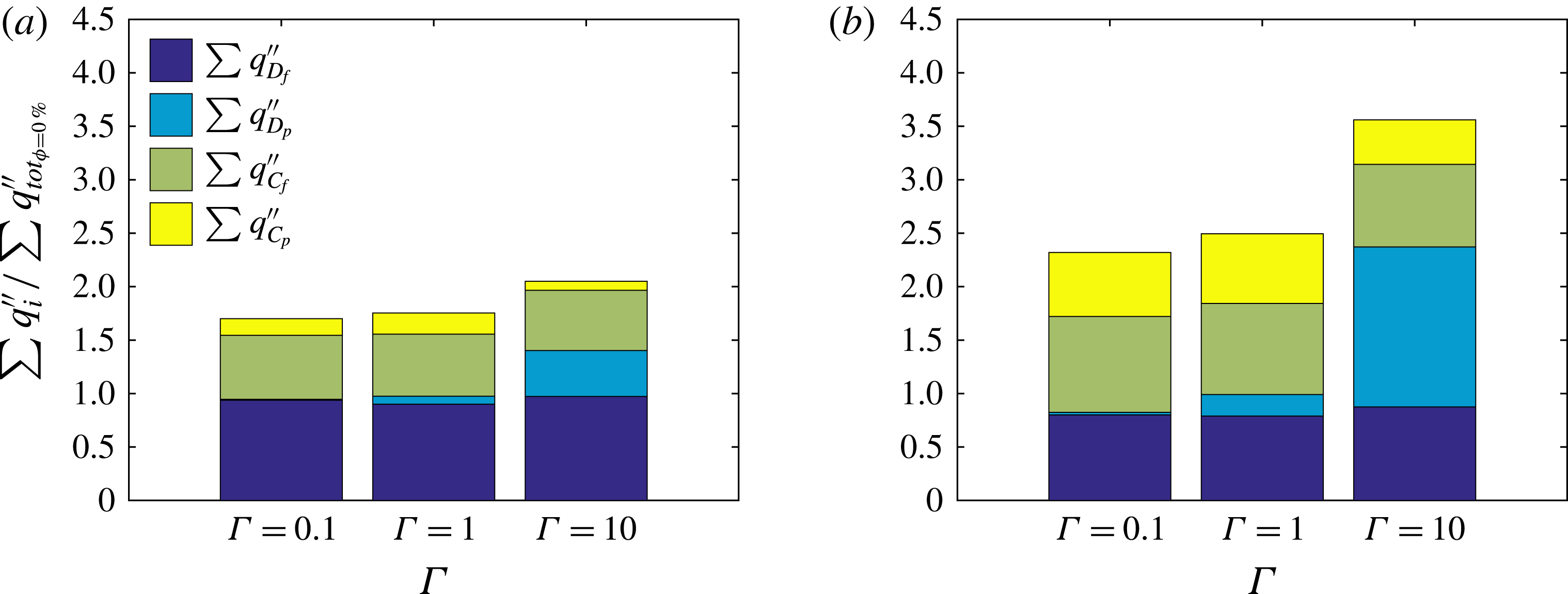
Figure 14. Wall-normal integral of the different terms defining the average heat flux across the channel, normalized by the total heat flux in single-phase flow for: (a)
 $\unicode[STIX]{x1D719}=10\,\%$
and (b)
$\unicode[STIX]{x1D719}=10\,\%$
and (b)
 $\unicode[STIX]{x1D719}=30\,\%$
.
$\unicode[STIX]{x1D719}=30\,\%$
.
The analysis of the averaged heat flux across the gap width between the planes (see (4.1)) is repeated here for the cases with different
 $\unicode[STIX]{x1D6E4}$
. The results are presented in figure 13(a–d) for
$\unicode[STIX]{x1D6E4}$
. The results are presented in figure 13(a–d) for
 $\unicode[STIX]{x1D719}=10\,\%$
and figure 13(e–h) for
$\unicode[STIX]{x1D719}=10\,\%$
and figure 13(e–h) for
 $\unicode[STIX]{x1D719}=30\,\%$
at
$\unicode[STIX]{x1D719}=30\,\%$
at
 $\unicode[STIX]{x1D6E4}=0.1$
,
$\unicode[STIX]{x1D6E4}=0.1$
,
 $10$
and
$10$
and
 $Re_{p}=0.5$
,
$Re_{p}=0.5$
,
 $16$
. As mentioned before, all terms in (4.1) are normalized with the total wall-normal heat flux.
$16$
. As mentioned before, all terms in (4.1) are normalized with the total wall-normal heat flux.
The data show that for the case at
 $Re_{p}=0.5$
and
$Re_{p}=0.5$
and
 $\unicode[STIX]{x1D6E4}=0.1$
, when the flow around the particles is in the Stokes regime, molecular diffusion in the fluid is the dominant contribution to the overall heat flux. The contribution from diffusion in the solid phase is small in this case owing to the low thermal diffusivity of the particles; the terms related to the velocity fluctuations play a very minor role because of the low particle Reynolds number and low level of fluctuations. Indeed, the fluid and particle fluctuations are almost negligible when
$\unicode[STIX]{x1D6E4}=0.1$
, when the flow around the particles is in the Stokes regime, molecular diffusion in the fluid is the dominant contribution to the overall heat flux. The contribution from diffusion in the solid phase is small in this case owing to the low thermal diffusivity of the particles; the terms related to the velocity fluctuations play a very minor role because of the low particle Reynolds number and low level of fluctuations. Indeed, the fluid and particle fluctuations are almost negligible when
 $Re_{p}=0.5$
. When
$Re_{p}=0.5$
. When
 $\unicode[STIX]{x1D6E4}=10$
, the diffusion in the solid is larger than that in the fluid only when the volume fraction
$\unicode[STIX]{x1D6E4}=10$
, the diffusion in the solid is larger than that in the fluid only when the volume fraction
 $\unicode[STIX]{x1D719}=30\,\%$
, except for a small region close to the wall, where the local solid volume fraction tends to zero.
$\unicode[STIX]{x1D719}=30\,\%$
, except for a small region close to the wall, where the local solid volume fraction tends to zero.
Finally, we consider inertial effects, the last two rows of figure 13 pertaining to the results at
 $Re_{p}=16$
. When the particle diffusivity is lower than the fluid one,
$Re_{p}=16$
. When the particle diffusivity is lower than the fluid one,
 $\unicode[STIX]{x1D6E4}=0.1$
, the fraction of heat diffusing through the solid particles is negligible and the fluctuations in the fluid and solid particles play a major role in the heat transfer process. Already at
$\unicode[STIX]{x1D6E4}=0.1$
, the fraction of heat diffusing through the solid particles is negligible and the fluctuations in the fluid and solid particles play a major role in the heat transfer process. Already at
 $\unicode[STIX]{x1D719}=10\,\%$
, the heat transfer due to the fluctuations in the fluid velocity is comparable to the heat diffusing in the fluid towards the centreline of the domain. At higher particle volume fractions,
$\unicode[STIX]{x1D719}=10\,\%$
, the heat transfer due to the fluctuations in the fluid velocity is comparable to the heat diffusing in the fluid towards the centreline of the domain. At higher particle volume fractions,
 $q_{C_{f}}^{\prime \prime }$
dominates over the other transport mechanisms except for a region close to the wall where the velocity and temperature fluctuations vanish. At the highest volume fraction investigated,
$q_{C_{f}}^{\prime \prime }$
dominates over the other transport mechanisms except for a region close to the wall where the velocity and temperature fluctuations vanish. At the highest volume fraction investigated,
 $\unicode[STIX]{x1D719}=30\,\%$
, the wall-normal heat transfer due to the combined effect of temperature and particle velocity fluctuations is almost equal to the heat diffusion in the fluid. For the cases with
$\unicode[STIX]{x1D719}=30\,\%$
, the wall-normal heat transfer due to the combined effect of temperature and particle velocity fluctuations is almost equal to the heat diffusion in the fluid. For the cases with
 $\unicode[STIX]{x1D6E4}=10$
, however, all four terms play an important role and none of them can be a priori discarded. At the lowest volume fraction,
$\unicode[STIX]{x1D6E4}=10$
, however, all four terms play an important role and none of them can be a priori discarded. At the lowest volume fraction,
 $\unicode[STIX]{x1D719}=10\,\%$
, the heat diffusion and the transport related to the fluid velocity fluctuations,
$\unicode[STIX]{x1D719}=10\,\%$
, the heat diffusion and the transport related to the fluid velocity fluctuations,
 $q_{D_{f}}^{\prime \prime }$
and
$q_{D_{f}}^{\prime \prime }$
and
 $q_{C_{f}}^{\prime \prime }$
, are dominant especially in the centre of the channel. On the contrary, the diffusion in the solid phase,
$q_{C_{f}}^{\prime \prime }$
, are dominant especially in the centre of the channel. On the contrary, the diffusion in the solid phase,
 $q_{D_{p}}^{\prime \prime }$
, dominates at higher volume fractions, except for the small region close to the wall where the local volume fraction approaches zero.
$q_{D_{p}}^{\prime \prime }$
, dominates at higher volume fractions, except for the small region close to the wall where the local volume fraction approaches zero.
The global contribution of each term to the steady-state heat flux is depicted in figure 14, where the results are normalized by the total heat flux in the absence of particles. Interestingly, the heat flux due to the particle velocity fluctuations reduces when
 $\unicode[STIX]{x1D6E4}=10$
. Indeed, as we discussed in the previous section, the ratio between the velocity and time scale of thermal diffusion inside the particles and transport with the particles (proportional to the particle velocity fluctuations) can affect the relative importance of these two transport mechanisms; for example, for
$\unicode[STIX]{x1D6E4}=10$
. Indeed, as we discussed in the previous section, the ratio between the velocity and time scale of thermal diffusion inside the particles and transport with the particles (proportional to the particle velocity fluctuations) can affect the relative importance of these two transport mechanisms; for example, for
 $\unicode[STIX]{x1D6E4}=10$
the velocity of thermal diffusion is significantly larger than for
$\unicode[STIX]{x1D6E4}=10$
the velocity of thermal diffusion is significantly larger than for
 $\unicode[STIX]{x1D6E4}=1$
, causing the particles to reach the surrounding fluid temperature fast in comparison to the particle’s own motion.
$\unicode[STIX]{x1D6E4}=1$
, causing the particles to reach the surrounding fluid temperature fast in comparison to the particle’s own motion.
The above results shed some light on the contribution of the solid-phase thermal diffusivity to the heat transfer in particle suspensions. We show that, in a suspension of solid particles with a lower thermal diffusivity than the fluid, the heat transfer through the suspension can become smaller than that in single-phase flow. However, as the inertia of the particles increases, the heat transfer can be enhanced by the wall-normal velocity fluctuations even in the presence of particles with lower diffusivity,
 $\unicode[STIX]{x1D6E4}<1$
. The results indicate that the thermal diffusivity of the solid phase is more important when the flow is in the Stokes regime and inertial effects are negligible.
$\unicode[STIX]{x1D6E4}<1$
. The results indicate that the thermal diffusivity of the solid phase is more important when the flow is in the Stokes regime and inertial effects are negligible.
5 Final remarks
We report results from interface-resolved direct numerical simulations (DNS) of plane Couette flow with rigid spherical particles. In this study, we focus on the heat transfer enhancement when varying particle Reynolds number, total volume fraction (number of particles) and the ratio between the particle and fluid thermal diffusivities. Simulations are performed using a numerical approach proposed in this study to address heat transfer in both phases. The numerical algorithm is based on an immersed boundary method (IBM) to resolve fluid–solid interactions, with lubrication and contact models for the short-range particle–particle (particle–wall) interactions. A volume-of-fluid (VoF) model is used to solve the heat transfer equation both inside and outside of the particles, enabling us to consider different thermal diffusivities in the two phases. In the current work we show how the ratio between the velocity and time scale of thermal diffusion inside the particles and transport with the particles (proportional to the particle velocity fluctuations) can affect the relative importance of these two transport mechanisms. For this purpose we consider similar
 $\unicode[STIX]{x1D70C}C_{p}$
for the particles and the fluid while changing the particle Reynolds number and the thermal diffusivity of the particles. Indeed, having different
$\unicode[STIX]{x1D70C}C_{p}$
for the particles and the fluid while changing the particle Reynolds number and the thermal diffusivity of the particles. Indeed, having different
 $\unicode[STIX]{x1D70C}\ast C_{p}$
between the particles and the fluid can change the ratio of the velocity and time scales, and therefore it will be very interesting also to distinguish the effect of
$\unicode[STIX]{x1D70C}\ast C_{p}$
between the particles and the fluid can change the ratio of the velocity and time scales, and therefore it will be very interesting also to distinguish the effect of
 $C_{p}$
and
$C_{p}$
and
 $K$
in future studies, using the same VoF approach with a slightly different discretization of the energy equation.
$K$
in future studies, using the same VoF approach with a slightly different discretization of the energy equation.
The results of the simulations show that the effective thermal diffusivity of the suspension increases linearly with the volume fraction of the particles at small particle Reynolds numbers, in agreement with the experimental and numerical findings in Metzger et al. (Reference Metzger, Rahli and Yin2013) for the Stokes regime, which serve as validation for the present method. We report that this correlation can predict well the effective thermal diffusivity of the suspension, up to approximately
 $Re_{p}=4$
, where the deviation from the correlation is less than
$Re_{p}=4$
, where the deviation from the correlation is less than
 $\pm 4\,\%$
. At high
$\pm 4\,\%$
. At high
 $Re_{p}$
, the almost-linear profile of effective thermal diffusivity changes to a curve, which is underpredicted and overpredicted by the correlation for low and high volume fractions, respectively.
$Re_{p}$
, the almost-linear profile of effective thermal diffusivity changes to a curve, which is underpredicted and overpredicted by the correlation for low and high volume fractions, respectively.
We also vary the ratio between the particle and fluid thermal diffusivities and show that the results are found to collapse reasonably well for vanishing inertia when rescaled with the conductivity of a composite estimated by the Lewis–Nielsen model (Nielsen Reference Nielsen1974). Inertial effects trigger an increase of the heat transfer, which is, in absolute value, more pronounced for
 $\unicode[STIX]{x1D6E4}=10$
. However, when scaling the data with the average conductivity of a composite, the increase due to inertial effects is relatively more important at
$\unicode[STIX]{x1D6E4}=10$
. However, when scaling the data with the average conductivity of a composite, the increase due to inertial effects is relatively more important at
 $\unicode[STIX]{x1D6E4}=0.1$
.
$\unicode[STIX]{x1D6E4}=0.1$
.
It should be noted that the increase of the effective thermal diffusivity with the addition of particles usually comes at the price of an increase in the effective viscosity of the flow, resulting in higher external power needed to drive the flow. We show in this study that for particle volume fractions lower than
 $10\,\%$
inertial effects (
$10\,\%$
inertial effects (
 $Re_{p}=16$
) increase the heat transfer more than the momentum transfer; in other words the enhancement in the effective thermal diffusivity of the suspension is more than the increase of the effective viscosity, which we denote as an efficient heat transfer enhancement. The increase of the effective thermal diffusivity is limited at low volume fractions. At higher volume fractions, instead, the increase of the effective viscosity exceeds the increase in effective thermal diffusivity.
$Re_{p}=16$
) increase the heat transfer more than the momentum transfer; in other words the enhancement in the effective thermal diffusivity of the suspension is more than the increase of the effective viscosity, which we denote as an efficient heat transfer enhancement. The increase of the effective thermal diffusivity is limited at low volume fractions. At higher volume fractions, instead, the increase of the effective viscosity exceeds the increase in effective thermal diffusivity.
To better understand the heat-transfer process, we ensemble-average the heat transfer equation and obtain four different contributions making up the total heat transfer: (i) transport associated with the particle motion; (ii) convection by fluid velocity; (iii) molecular diffusion in the solid phase (solid conduction); and (iv) molecular diffusion in the fluid phase (fluid conduction). The analysis shows that the increase of the effective conductivity observed at finite inertia can be associated with an increase of the transport associated with fluid and particle velocity. Interestingly, the total contribution of the solid conduction term reduces when increasing the particle Reynolds number. This can be explained by the ratio between the time scale of molecular diffusion in the solid and of the transport by particle motions. As particles move faster, conduction inside the solid becomes negligible. Given the small contribution of the solid conduction term at high particle Reynolds numbers, we expect that decreasing the particle thermal diffusivity does not have a large influence on the total heat transfer. Indeed, the results of the simulations with different thermal diffusivities match the mentioned expectation, as the effective thermal diffusivity at
 $\unicode[STIX]{x1D6E4}=0.1$
is close to that at
$\unicode[STIX]{x1D6E4}=0.1$
is close to that at
 $\unicode[STIX]{x1D6E4}=1$
. On the other hand, a particle thermal diffusivity higher than that of the fluid significantly increases the effective heat transfer.
$\unicode[STIX]{x1D6E4}=1$
. On the other hand, a particle thermal diffusivity higher than that of the fluid significantly increases the effective heat transfer.
We investigate in this study the effect of particle Reynolds number, total volume fraction (number of particles) and the thermal diffusivity of the particles on the effective thermal diffusivity of the suspension. However, the effect of particle shape on the heat transfer still remains unexplored, something that may be addressed in the near future. This is potentially interesting, as particles of different shapes may have different distributions across the channel. We show in this study that for the inertial cases, where the convection by the fluid plays an important role in the heat transfer, the migration of the particles away from the wall and therefore near-wall depletion further enhances the effective heat transfer. In the present study, we obtain depletion of the near-wall region by artificially imposing zero angular velocity on the motion of particles, an effect that may be induced by a different particle shape.
Acknowledgement
L.B. and M.N.A. acknowledge financial support by the European Research Council, Grant No. ERC-2013-CoG-616186, TRITOS. O.A. acknowledges the financial support of Shiraz University for the granted sabbatical leave. Computer time has been provided by SNIC (the Swedish National Infrastructure for Computing).
Appendix A. Different contributions to the total heat transfer
In this section we examine the heat flux in suspension mixtures by phase-ensemble-averaging the heat transfer equation using the framework developed and employed in Marchioro, Tanksley & Prosperetti (Reference Marchioro, Tanksley and Prosperetti1999), Zhang & Prosperetti (Reference Zhang and Prosperetti2010) and Picano et al. (Reference Picano, Breugem and Brandt2015), and find the different contributions to the total heat transfer reported in the main text. We define the phase indicator
 $\unicode[STIX]{x1D709}$
, whose value varies between
$\unicode[STIX]{x1D709}$
, whose value varies between
 $0$
and
$0$
and
 $1$
based on the solid fraction in the considered volume. Defining the phase-ensemble average
$1$
based on the solid fraction in the considered volume. Defining the phase-ensemble average
 $\langle ~\rangle$
as the ensemble average (implicitly) conditioned to the considered phase, the local volume fraction is defined as
$\langle ~\rangle$
as the ensemble average (implicitly) conditioned to the considered phase, the local volume fraction is defined as
 $$\begin{eqnarray}\displaystyle \unicode[STIX]{x1D6F7}=\langle \unicode[STIX]{x1D709}\rangle . & & \displaystyle\end{eqnarray}$$
A generic observable of the combined phase,
 $O_{c}$
, can be constructed in terms of
$O_{c}$
, can be constructed in terms of
 $O_{p}$
and
$O_{p}$
and
 $O_{f}$
(the same observable inside the particles and in the fluid phase), using the phase indicator
$O_{f}$
(the same observable inside the particles and in the fluid phase), using the phase indicator
 $\unicode[STIX]{x1D709}$
. The phase-ensemble average of
$\unicode[STIX]{x1D709}$
. The phase-ensemble average of
 $O_{c}$
is
$O_{c}$
is
 $$\begin{eqnarray}\displaystyle \langle O_{c}\rangle =\langle \unicode[STIX]{x1D709}O_{p}+(1-\unicode[STIX]{x1D709})O_{f}\rangle =\unicode[STIX]{x1D6F7}\langle O_{p}\rangle +(1-\unicode[STIX]{x1D6F7})\langle O_{f}\rangle , & & \displaystyle\end{eqnarray}$$
where we use the subscript inside the brackets to indicate the phase conditioning.
The differential heat transfer equation,
 $$\begin{eqnarray}\displaystyle \unicode[STIX]{x1D70C}C_{p}\frac{\text{D}T}{\text{D}t}=\unicode[STIX]{x1D735}\boldsymbol{\cdot }(k\unicode[STIX]{x1D735}T), & & \displaystyle\end{eqnarray}$$
can be rewritten in terms of both phases as
 $$\begin{eqnarray}\displaystyle \unicode[STIX]{x1D709}(\unicode[STIX]{x1D70C}C_{p})_{p}\frac{\text{D}T_{p}}{\text{D}t}+(1-\unicode[STIX]{x1D709})(\unicode[STIX]{x1D70C}C_{p})_{f}\frac{\text{D}T_{f}}{\text{D}t}=\unicode[STIX]{x1D735}\boldsymbol{\cdot }\left[\unicode[STIX]{x1D709}k_{p}\unicode[STIX]{x1D735}T_{p}+(1-\unicode[STIX]{x1D709})k_{f}\unicode[STIX]{x1D735}T_{f}\right]. & & \displaystyle\end{eqnarray}$$
Phase-ensemble-averaging (A 4) and using (A 1) and (A 2) results in
 $$\begin{eqnarray}\displaystyle & & \displaystyle \unicode[STIX]{x1D6F7}(\unicode[STIX]{x1D70C}C_{p})_{p}\left[\left\langle \frac{\unicode[STIX]{x2202}T_{p}}{\unicode[STIX]{x2202}t}\right\rangle +\langle \boldsymbol{u}_{p}\boldsymbol{\cdot }\unicode[STIX]{x1D735}T_{p}\rangle \right]+\left(1-\unicode[STIX]{x1D6F7}\right)(\unicode[STIX]{x1D70C}C_{p})_{f}\left[\left\langle \frac{\unicode[STIX]{x2202}T_{f}}{\unicode[STIX]{x2202}t}\right\rangle +\langle \boldsymbol{u}_{f}\boldsymbol{\cdot }\unicode[STIX]{x1D735}T_{f}\rangle \right]\nonumber\\ \displaystyle & & \displaystyle \qquad =\unicode[STIX]{x1D735}\boldsymbol{\cdot }\left[\unicode[STIX]{x1D6F7}k_{p}\langle \unicode[STIX]{x1D735}T_{p}\rangle +\left(1-\unicode[STIX]{x1D6F7}\right)k_{f}\langle \unicode[STIX]{x1D735}T_{f}\rangle \right].\end{eqnarray}$$
Next we decompose temperature and velocity into the average and fluctuating part (
 $\boldsymbol{u}=\boldsymbol{U}+\boldsymbol{u}^{\prime }$
and
$\boldsymbol{u}=\boldsymbol{U}+\boldsymbol{u}^{\prime }$
and
 $T=\overline{T}+T^{\prime }$
) and consider the mean of these quantities. With the above decomposition, equation (A 5) can be rewritten as
$T=\overline{T}+T^{\prime }$
) and consider the mean of these quantities. With the above decomposition, equation (A 5) can be rewritten as
 $$\begin{eqnarray}\displaystyle & & \displaystyle \unicode[STIX]{x1D6F7}(\unicode[STIX]{x1D70C}C_{p})_{p}\left[\boldsymbol{U}_{p}\boldsymbol{\cdot }\unicode[STIX]{x1D735}\overline{T}_{p}+\langle \boldsymbol{u}_{p}^{\prime }\boldsymbol{\cdot }\unicode[STIX]{x1D735}T_{p}^{\prime }\rangle \right]+(1-\unicode[STIX]{x1D6F7})(\unicode[STIX]{x1D70C}C_{p})_{f}\left[\boldsymbol{U}_{f}\boldsymbol{\cdot }\unicode[STIX]{x1D735}\overline{T}_{f}+\langle \boldsymbol{u}_{f}^{\prime }\boldsymbol{\cdot }\unicode[STIX]{x1D735}T_{f}^{\prime }\rangle \right]\nonumber\\ \displaystyle & & \displaystyle \qquad =\unicode[STIX]{x1D735}\boldsymbol{\cdot }\left[\unicode[STIX]{x1D6F7}k_{p}\langle \unicode[STIX]{x1D735}T_{p}\rangle +(1-\unicode[STIX]{x1D6F7})k_{f}\langle \unicode[STIX]{x1D735}T_{f}\rangle \right].\end{eqnarray}$$
Assuming
 $(\unicode[STIX]{x1D70C}C_{p})_{p}=(\unicode[STIX]{x1D70C}C_{p})_{f}$
and exploiting the symmetries in the two homogeneous directions, the projection of (A 6) in the inhomogeneous wall-normal direction
$(\unicode[STIX]{x1D70C}C_{p})_{p}=(\unicode[STIX]{x1D70C}C_{p})_{f}$
and exploiting the symmetries in the two homogeneous directions, the projection of (A 6) in the inhomogeneous wall-normal direction
 $y$
gives
$y$
gives
 $$\begin{eqnarray}\displaystyle \frac{\text{d}}{\text{d}y}\left[-\unicode[STIX]{x1D6F7}\langle v_{p}^{\prime }T_{p}^{\prime }\rangle -(1-\unicode[STIX]{x1D6F7})\langle v_{f}^{\prime }T_{f}^{\prime }\rangle +\unicode[STIX]{x1D6F7}\unicode[STIX]{x1D6FC}_{p}\left\langle \frac{\text{d}T_{p}}{\text{d}y}\right\rangle +(1-\unicode[STIX]{x1D6F7})\unicode[STIX]{x1D6FC}_{f}\left\langle \frac{\text{d}T_{f}}{\text{d}y}\right\rangle \right]=0, & & \displaystyle\end{eqnarray}$$
where
 $\unicode[STIX]{x1D6FC}_{p}=k_{p}/(\unicode[STIX]{x1D70C}C_{p})_{p}$
and
$\unicode[STIX]{x1D6FC}_{p}=k_{p}/(\unicode[STIX]{x1D70C}C_{p})_{p}$
and
 $\unicode[STIX]{x1D6FC}_{f}=k_{f}/(\unicode[STIX]{x1D70C}C_{p})_{f}$
.
$\unicode[STIX]{x1D6FC}_{f}=k_{f}/(\unicode[STIX]{x1D70C}C_{p})_{f}$
.
Finally, integrating (A 7) in the wall-normal direction results in the following equation for the total heat flux
 $q_{tot}^{\prime \prime }$
:
$q_{tot}^{\prime \prime }$
:
 $$\begin{eqnarray}\displaystyle q_{tot}^{\prime \prime }=-\unicode[STIX]{x1D6F7}\langle v_{p}^{\prime }T_{p}^{\prime }\rangle -(1-\unicode[STIX]{x1D6F7})\langle v_{f}^{\prime }T_{f}^{\prime }\rangle +\unicode[STIX]{x1D6F7}\unicode[STIX]{x1D6FC}_{p}\left\langle \frac{\text{d}T_{p}}{\text{d}y}\right\rangle +(1-\unicode[STIX]{x1D6F7})\unicode[STIX]{x1D6FC}_{f}\left\langle \frac{\text{d}T_{f}}{\text{d}y}\right\rangle . & & \displaystyle\end{eqnarray}$$


