2.1. Simulation setup

In all the previously cited works, different resolution levels and a large variety of analyses have been performed on the same configuration, providing an extensive framework for validation. The canonical problem consists of a supersonic, fully-turbulent, boundary layer interacting with a $24^{\circ }$ compression/expansion ramp. The computational domain (see figure 1) has been parametrised using the $99$ % thickness of the incoming boundary layer (here denoted as $\delta$). The classical geometry of the present configuration is commonly limited to the compression ramp only. The subsequent expansion corner has been added to study the effect of strong expansions on the turbulence.

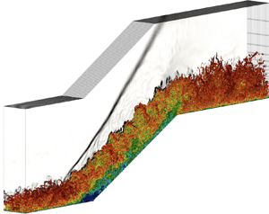
Figure 1. Q-criterion contours coloured by velocity magnitude ($Q=1.0 u_{\infty }^{2}/\delta ^{2}$). In the background, numerical Schlieren is displayed to highlight the primary shock wave. Here, $\delta$ denotes incoming boundary layer thickness.

As geometrical reference, the origin is located at the corner of the compression ramp and the $x$-coordinates are measured starting from this point following wall-tangent directions. In agreement with the DNS by Priebe & Martín (Reference Priebe and Martín2012), the reference supersonic boundary layer has been evaluated at $x=-8\delta$. Upstream of this location, the generation of the turbulent boundary layer itself takes place. In the work by Priebe & Martín (Reference Priebe and Martín2012), a secondary simulation based on recycling/rescaling has been used in order to prescribe a realistic inlet condition at $x=-8\delta$. In the present simulation, instead, an extended domain has been considered, in which the digital filter technique for turbulence generation by Klein, Sadiki & Janicka (Reference Klein, Sadiki and Janicka2003) has been applied at $x=-20\delta$. A weakly Riemann-based, non-reflective, far-field boundary condition has been enforced on the upper boundary. Periodic boundary conditions have been prescribed in the spanwise direction. Notice that the spanwise extent of the domain has been chosen to match previous similar studies (Wu & Martín Reference Wu and Martín2007; Li et al. Reference Li, Fu, Ma and Liang2010; Priebe & Martín Reference Priebe and Martín2012; Tong et al. Reference Tong, Tang, Yu, Zhu and Li2017a,Reference Tong, Yu, Tang and Lib).

The main flow properties of the boundary layer are listed in table 1.

Table 1. Characteristic of the incoming boundary layer.

The Reynolds number is defined as ${Re}_{\theta }=u_{\infty }\theta /\nu _{\infty }$, where $\theta$ represents the momentum thickness, $u_{\infty }$ the free stream velocity and $\nu _{\infty }$ the kinematic viscosity in the free stream flow. The Kármán number is defined as $\delta ^{+}=\delta u_{\tau }/\nu _{w}$, where $u_{\tau }$ denotes the friction velocity and $\nu _{w}$ the kinematic viscosity at the wall. Finally, $\delta ^{*}$ indicates the displacement thickness and $H=\delta ^{*}/\theta$ the shape factor. The kinematic viscosity, defined as $\nu =\mu (T)/\rho$, varies over the domain due to the direct dependence on density and implicit dependence on the temperature through the dynamic viscosity, here modelled using Sutherland's law:

(2.1)\begin{equation} \mu=\mu_{{ref}}\left(\frac{T}{T_{{ref}}}\right)^{3/2} \frac{(T_{{ref}}+\mathcal{S})}{(T+\mathcal{S})}, \end{equation}

with $\mu _{{ref}}=1.834 \times 10^{-5}\ {\rm kg\ \ m}^{-1}\ {\rm s}^{-1}$, $T_{{ref}}=291.15\ {\rm K}$ and $\mathcal {S}=120\ {\rm K}$. No-slip isothermal conditions have been applied to the wall faces. Finally, the temperature at the wall has been enforced as $T_{w}=307\ {\rm K}$, corresponding to approximately $1.14$ the recovery temperature. The free stream density has been set to the nominal value $\rho _{\infty }=7.7 \times 10^{-2} \ {\rm kg\ \ m}^{-3}$.

Regarding the turbulent inlet condition, many different approaches have been proposed in the literature of SWTI to prescribe turbulent inflow generation (see Wu (Reference Wu2017) for an extensive summary). Using the Klein et al. (Reference Klein, Sadiki and Janicka2003) digital filter technique, generalised and validated to the present numerical set-up (Pinto & Lodato Reference Pinto and Lodato2019; Lodato, Tonicello & Pinto Reference Lodato, Tonicello and Pinto2021), the mean profiles, to which perturbations are superposed, have been evaluated using closed-form relations involving van Driest transformed velocity as described by Touber (Reference Touber2010). Given the correlation tensor of the fluid velocity and typical length scales of the desired turbulence field, realistic velocity fluctuations are prescribed at the inlet boundaries, far enough from the flow zone of interest. The values of the correlation tensor have been extrapolated from a turbulent boundary layer DNS performed by Pirozzoli & Bernardini (Reference Pirozzoli and Bernardini2011b) at a similar Reynolds number. Finally, density and temperature fluctuations have been imposed using the strong Reynolds analogy (SRA).

Details regarding the 6th-order accurate numerical discretisation are listed in table 2. The number of total degrees of freedom (DoF) has been chosen in order to match the accuracy of the DNS by Priebe & Martín (Reference Priebe and Martín2012). As is common practice for high-order spectral element schemes, the grid spacings in table 2 have been evaluated using the length of the elements along each direction divided by the order of approximation (denoted as $N$). Wall resolution is enforced by locating the first solution point at $y^{+}\approx 0.3$ and the entire first element within the viscous sublayer ($y^{+} < 10$). The mesh spacing along the streamwise direction varies between ${\rm \Delta} x^{+}=4.75$ and ${\rm \Delta} x^{+}=15$, whereas the spanwise mesh spacing is ${\rm \Delta} z^{+}=4.2$. Such choices are particularly common in the numerical simulation of low- Reynolds-number turbulent boundary layers. To further validate the resolution of the present computation, the Kolmogorov length scale has been estimated a posteriori as $\eta = (\nu ^{3}/\varepsilon )^{1/4}$, with $\varepsilon = 2\langle {\nu S_{ij}^{d} ({\partial u_{i}}/{\partial u_{j}})}\rangle$. The ratio between the effective grid spacing $\varDelta = ({\rm \Delta} x \times {\rm \Delta} y \times {\rm \Delta} z)^{1/3}$ and the Kolmogorov length scale $\eta$ was found to be approximatively equal to unity upstream of the shock, and never larger than $6$ downstream of the interaction region. As shown by Pirozzoli, Bernardini & Grasso (Reference Pirozzoli, Bernardini and Grasso2008), the small-scale eddies in wall-bounded turbulence are characterised by a typical length scale of 5–6 times $\eta$. It is worthwhile mentioning that the use of the resolved flow to evaluate its own characteristic scales gives only an estimation of the order of magnitude of the Kolmogorov length scale. It is also commonly known that the primary limiting factor of wall-bounded turbulent flows is driven mainly by the accurate prediction of the viscous sublayer (see, for instance, Sayadi, Hamman & Moin Reference Sayadi, Hamman and Moin2013), which is properly resolved by the present computation. Consequently, based on such considerations, the prescribed resolution is expected to be sufficiently accurate to properly resolve all the relevant scales of the turbulent structures for the present configuration.

Table 2. Numerical discretisation details, where $N$ denotes order of approximation, $N_{x}, N_{y}, N_{z}$ denote the numbers of elements along the streamwise, wall-normal and spanwise directions, respectively, and ${\rm \Delta} x^{+}, {\rm \Delta} y^{+}, {\rm \Delta} z^{+}$ denote the wall-normalised grid spacings.

The computational domain (figure 2) has been enlarged with respect to most of the previously cited works based on recycling/rescaling techniques. Indeed, the inlet forcing method for turbulence injection necessitates a certain length to develop the desired boundary layer statistical properties, which can vary considerably depending on the specific turbulence injection techniques. The recovery distance can vary from approximately $2/3 \delta$ (Adler et al. Reference Adler, Gonzalez, Stack and Gaitonde2018) up to $15 \delta$ (Morgan et al. Reference Morgan, Larsson, Kawai and Lele2011, Reference Morgan, Duraisamy, Nguyen, Kawai and Lele2013). In the present work, the reference fully-developed boundary layer is evaluated at $x=-8\delta$, which is located $12 \delta$ downstream from the inlet boundary. As will be discussed more thoroughly in the following sections of the paper, such a distance has been shown to be sufficiently long to provide good first- and second-order statistics of the turbulent velocity field. Finally, relevant statistics have been gathered every $0.025 \delta /u_{\infty }$ s for approximatively $1000 \delta /u_{\infty }$ s, which is commonly considered enough time to obtain a reliable temporal convergence for the present configuration (Wu & Martín Reference Wu and Martín2007; Li et al. Reference Li, Fu, Ma and Liang2010; Priebe & Martín Reference Priebe and Martín2012).

Figure 2. Compression/expansion ramp: computational grid. Here, $\delta$ denotes incoming boundary layer thickness.

2.2. Shock capturing

The compressible Navier–Stokes equations are solved using the spectral difference method for unstructured spatial discretisation (Kopriva & Kolias Reference Kopriva and Kolias1996; Sun et al. Reference Sun, Wang and Liu2007; Jameson Reference Jameson2010; Jameson, Vincent & Castonguay Reference Jameson, Vincent and Castonguay2012). Letting $\rho$ be the density, $u_i$ the velocity components, and $E$ the specific total energy (internal plus kinetic), these read

(2.2)$$\begin{gather} \frac{\partial{\rho}}{\partial{t}} +\frac{\partial{}}{\partial{x_{j}}}(\rho u_{j}) = 0, \end{gather}$$

(2.3)$$\begin{gather}\frac{\partial{}}{\partial{t}}(\rho u_{i}) +\frac{\partial{}}{\partial{x_{j}}}(\rho u_{i} u_{j} +p \delta_{ij}) = \frac{\partial{}}{\partial{x_{j}}}(\sigma_{ij}), \end{gather}$$

(2.4)$$\begin{gather}\frac{\partial{}}{\partial{t}}(\rho E) +\frac{\partial{}}{\partial{x_{j}}}[(\rho E + p) u_{j}] = \frac{\partial{}}{\partial{x_{j}}}(\sigma_{ij} u_{i})-\frac{\partial{q_{j}}}{\partial{x_{j}}}, \end{gather}$$

where $\delta _{ij}$ is the Kronecker delta, $\sigma _{ij}$ is the viscous stress tensor, and $q_j$ is the heat flux vector. This last is computed via the Fourier law as $q_j = -\kappa \,\partial T / \partial x_j$, where $\kappa$ is thermal conductivity and $T$ is temperature. The above equations are closed using the ideal gas state equation

(2.5a,b)\begin{equation} p = \rho R T,\quad\rho E = \frac{p}{\gamma-1} + \frac{1}{2}\rho u_k u_k, \end{equation}

where $R$ is the gas constant and $\gamma = c_p/c_v$ is the specific heat ratio.

Shock waves will often represent an under-resolved feature of the flow field, and artificial terms are necessary for their numerical description. Consequently, the term ‘direct numerical simulation’ is here strictly restricted to the scales of turbulence and not to the whole spectrum of scales characterising the physics of the problem. See the works by Margolin (Margolin Reference Margolin2019; Margolin & Plesko Reference Margolin and Plesko2019) for a deeper discussion on artificial viscosity and SGS modelling.

In this work, the shock-capturing technique is based on the subcell shock- capturing method with modal sensors first proposed by Persson & Peraire (Reference Persson and Peraire2006) within a discontinuous Galerkin framework. The spectral behaviour of the resolved variables is evaluated along each direction in order to detect discontinuities in the flow field. The characteristic-based sensor proposed recently by Lodato (Reference Lodato2019a,Reference Lodatob) has been used. Once shock waves are located efficiently, they can be regularised properly using an artificial viscosity (AV) approach based on the bulk viscosity, similar to the one developed by Fernandez et al. (Reference Fernandez, Nguyen and Peraire2018b) and Fernandez, Nguyen & Peraire (Reference Fernandez, Nguyen and Peraire2018a). The artificial terms, added to the compressible Navier–Stokes equations, are based on an augmentation of physical fluid viscosities and diffusivities. Accordingly, considering a Newtonian fluid under Stokes’ hypothesis, the viscous stress tensor and the heat flux become

(2.6)\begin{equation} \sigma_{ij} = 2\mu S^{d}_{ij} + \beta_{{AV}}\,\frac{\partial{u_{k}}}{\partial{x_{k}}}\,\delta_{ij}, \end{equation}

where $S_{ij}^{d}$ indicates the deviatoric part of the strain-rate tensor

(2.7)\begin{equation} S_{ij}^{d}= \frac{1}{2}\left (\frac{\partial{u_{i}}}{\partial{x_{j}}}+\frac{\partial{u_{j}}}{\partial{x_{i}}}\right )-\frac{1}{3}\,\frac{\partial{u_{k}}}{\partial{x_{k}}}\,\delta_{ij}, \end{equation}

and

(2.8a,b)\begin{equation} q_{j}={-}(\kappa+\kappa_{{AV}})\frac{\partial{T}}{\partial{x_{j}}}, \quad \kappa_{{AV}}=\frac{\beta_{{AV}}c_{p}}{Pr_{\beta}}, \end{equation}

where $Pr_{\beta }$ is expressed dynamically as a function of the local Mach number according to the equation

(2.9)\begin{equation} Pr_{\beta}=Pr \{ 1+\exp[{-}4(Ma(\boldsymbol{x})-Ma_{{thr}})]\}. \end{equation}

The parameter $Ma_{{thr}}$ has been set to $3$, to avoid the addition of unnecessary thermal dissipation for low-Mach-number regions of the flow. This approach has been reported recently as a good compromise to capture the expected entropy overshot within the shock zone (Tonicello et al. Reference Tonicello, Lodato and Vervisch2020).

It was found necessary to improve this artificial viscosity model in the case of wall-bounded turbulent flows. While eddy-viscosity, by definition, vanishes at wall boundaries, as dictated by the turbulent boundary layer theory, the artificial viscosity has no constraint from this point of view. However, it is common practice to turn off the artificial viscosity at wall faces (Kawai et al. Reference Kawai, Shankar and Lele2010). Accordingly, to avoid the unnecessary activation of the artificial viscosity close to the wall, a modification of the sensor proposed by Ducros et al. (Reference Ducros, Ferrand, Nicoud, Weber, Darracq, Gacherieu and Poinsot1999) has been coupled with the baseline modal shock detection procedure. The elementwise constant shock sensor by Persson & Peraire (Reference Persson and Peraire2006) ($s_{{modal}}$) has been modified as follows:

(2.10)\begin{equation} s_{e}=s_{{modal}} \times \frac{[0.5(\lvert\langle{\partial{u_{k}}/\partial{x_{k}}}\rangle\rvert -\langle{\partial{u_{k}}/\partial{x_{k}}}\rangle)] ^{2}}{\langle{\partial{u_{k}}/\partial{x_{k}}}\rangle^{2}+ \langle{\sqrt{\omega_{k} \omega_{k}}}\rangle^{2}+\epsilon}, \end{equation}

where $\langle {\cdot }\rangle$ denotes elementwise averaging, $\omega _{i}=\varepsilon _{ijk}(\partial u_{k}/\partial x_{j})$ indicates the $i$th component of the vorticity vector, and $\epsilon$ is a constant of order machine epsilon squared. (To define the vorticity vector, the Levi–Civita symbol has been introduced, denoted as $\varepsilon _{ijk}$.) The present modification has been tested already in the same numerical framework for the simulation of transonic aerofoils (Tonicello, Lodato & Vervisch Reference Tonicello, Lodato and Vervisch2022). The proposed correction also prevents the activation of the artificial viscosity in strongly vortical regions characterised by negligible volumetric compressions. It is, in fact, well-known that excessively large values of bulk viscosity can deteriorate considerably the dilatation field in highly compressible regions (Kawai et al. Reference Kawai, Shankar and Lele2010; Tonicello et al. Reference Tonicello, Lodato and Vervisch2020).

In addition to the shock-capturing numerical approach, a positivity-preserving scheme developed by Zhang & Shu (Reference Zhang and Shu2010), adapted to the spectral difference scheme (Lodato, Vervisch & Clavin Reference Lodato, Vervisch and Clavin2016, Reference Lodato, Vervisch and Clavin2017; Lodato Reference Lodato2019a), has been employed to fully secure the stability of the simulation. The impact on the flow physics of both the shock-capturing and the positivity-preserving schemes are discussed thereafter. More detailed presentations of the shock-capturing technique and the positivity-preserving scheme have been included in Appendices B and C, respectively.

3.1. Wall coefficients and mean profiles

In order to validate the proposed DNS, the averaged friction coefficient and wall pressure have been computed and compared with previous simulations and experimental data of the same configuration in figure 3. In many other works, a perfect agreement within the rich literature of compression ramp simulations has proven to be a very difficult task to achieve. This is commonly true not only in the detached region of the flow, which can be very challenging to be accurately predicted, but also in the upstream region where large deviations of the skin friction coefficient are normally reported in the literature. To highlight such a tendency, the DNS by Zhu et al. (Reference Zhu, Yu, Tong and Li2017) along with experimental data by Ringuette et al. (Reference Ringuette, Bookey, Wyckham and Smits2009) have been added to figure 3. The simulation by Zhu et al. (Reference Zhu, Yu, Tong and Li2017) was performed under the same conditions as the experiments by Ringuette et al. (Reference Ringuette, Bookey, Wyckham and Smits2009) and DNS by Wu & Martín (Reference Wu and Martín2007), which were characterised by a slightly smaller Reynolds number with respect to the present computation (namely, ${Re}_{\theta } =2400$). Another relevant difference can be identified in the upstream boundary layer: the DNS performed by Zhu et al. (Reference Zhu, Yu, Tong and Li2017) did not rely on any artificial injection of turbulence. In fact, the full laminar-to-turbulent transition of the incoming boundary layer was explicitly simulated using a blow-and-suction disturbance technique.

Figure 3. Averaged (a) friction coefficient and (b) wall pressure, along the streamwise direction. Solid line, present simulation; dashed line, DNS by Zhu et al. (Reference Zhu, Yu, Tong and Li2017), dashed-dotted line, DNS by Priebe & Martín (Reference Priebe and Martín2012). Black circle, measurements by Ringuette et al. (Reference Ringuette, Bookey, Wyckham and Smits2009).

In figure 3(a), in the upstream region, the friction coefficient is slightly higher than the reference DNS by Priebe & Martín (Reference Priebe and Martín2012), whereas the simulation by Zhu et al. (Reference Zhu, Yu, Tong and Li2017) reports an even larger value. The experimental separation point is much better predicted by both Zhu et al. (Reference Zhu, Yu, Tong and Li2017) and the present simulation rather than by Priebe & Martín (Reference Priebe and Martín2012). Furthermore, both simulations tend to provide smaller values of the friction coefficient in the downstream region, in agreement with the experimental location of the reattachment point. In figure 3(b), the computed wall pressure profile follows nicely the one obtained by Zhu et al. (Reference Zhu, Yu, Tong and Li2017), which departs from the DNS by Priebe & Martín (Reference Priebe and Martín2012) within the interaction region around $-3 < x/\delta < 0$.

In order to assess the quality of the incoming boundary layer, mean profiles along wall-normal planes at different locations have been extracted. First, in figure 4, velocity profiles have been evaluated before the interaction with the shock wave ($x=-3 \delta$) and after ($x=4 \delta$). Second, in figure 5, the van Driest transformed streamwise velocity and the normalised Reynolds stresses at $x=-8 \delta$ are shown. In both panels of figure 5, the first $6$ solution points of the high-order discretisation are shown to highlight wall resolution. Notice that the first element is entirely contained in the viscous sublayer ($y^{+} < 10$). The van Driest transformed velocity follows accurately the experimental data in the log region, whereas some small differences with respect to the reference DNS are visible, in particular in the buffer layer.

Figure 4. Tangential velocity profiles along the wall-normal direction. (a) $x=-3 \delta$. Solid line, present simulation; dashed line, DNS by Priebe & Martín (Reference Priebe and Martín2012). (b) $x=4 \delta$. Solid line, present simulation; dashed line, DNS by Wu & Martín (Reference Wu and Martín2007); symbols, experimental data by Ringuette et al. (Reference Ringuette, Bookey, Wyckham and Smits2009); the streamwise velocity is normalised by the outer velocity $u_{e}$ downstream of the main shock.

Figure 5. (a) Van Driest (VD) transformed streamwise velocity at $x=-8 \delta$. Solid line, present simulation; dashed line, DNS by Wu & Martín (Reference Wu and Martín2007); symbols, experimental data by Ringuette et al. (Reference Ringuette, Bookey, Wyckham and Smits2009); dash-dotted line, $u_{VD}^{+} = y^{+}$ and $u_{VD}^{+} = 5.25 + \log (y^{+})/0.41$. (b) Normalised Reynolds stresses at $x=-8 \delta$. Solid line, present simulation; dashed line, DNS by Pirozzoli & Bernardini (Reference Pirozzoli and Bernardini2011b).

At $x=-3\delta$, the profile extracted from the present simulation shows a perfect agreement with the reference DNS. Downstream of the shock-interaction region, instead, some discrepancies can be seen, where a much better agreement with the experimental data by Ringuette et al. (Reference Ringuette, Bookey, Wyckham and Smits2009) has been obtained. Similar results in the detached region have been reported only by Kokkinakis et al. (Reference Kokkinakis, Drikakis, Ritos and Spottswood2020) using a $9$th order WENO scheme. In the same work, different schemes were employed and compared. Compared to lower order methods, the $9$th order WENO scheme resulted in higher values of the skin friction in the upstream boundary layer and smaller ones in the downstream region, in agreement with the results shown in figure 3(a).

Finally, the main features of the incoming boundary layer are summarised in table 3. Most of them are in fairly good agreement with the reference values of Priebe's simulation.

Table 3. Characteristics of the incoming boundary layer: reference versus computed.

3.2. Probes

The main variables have been collected over the simulated time through virtual probes located in regions characterised by different thermodynamic states and turbulence structure (see figure 6). Subsequently, temporal and spatial kinetic energy spectra have been related using Taylor's hypothesis. All the probes have been taken far enough from the wall, in order to make Taylor's hypothesis reasonably realistic. The first probe has been located in the log region of the incoming boundary layer, and the second in the detached flow downstream of the interaction with the shock wave. The kinetic energy spectra, computed using Taylor's hypothesis, are shown in figure 7(a). In addition, due to the periodic conditions along $z$, the kinetic energy spectra in the spanwise direction have been evaluated at the same locations; they are shown in figure 7(b). To reduce numerical noise, the spatial kinetic energy spectra have been computed at multiple time steps and subsequently averaged.

Figure 6. Probe locations. In the background, instantaneous normalised velocity magnitude field.

Figure 7. Kinetic energy spectra. Dashed line, $x=-8\delta$; solid line, $x=4\delta$. $\mathbb {E}$ denotes the kinetic energy Fourier spectrum of the velocity signal: (a) applying Taylor's hypothesis to temporal signals; (b) along $z$ ($y=0.7\delta$), where the vertical dashed line represents the Nyquist grid wavenumber. Here, $\kappa$ represents the wavenumber, which is evaluated along the spanwise direction as $\kappa _{z} = 0.5/z$ and, using Taylor's hypothesis, as $\kappa =2 {\rm \pi}f/\langle {\|\boldsymbol {u}\|}\rangle$, with $f$ the temporal frequency of the time signal. Both spectra are normalised by the first mode.

The inertial range is clearly visible in all the spectra, followed by a steeper viscous range where viscous dissipation takes place. Notice that no accumulation of kinetic energy in the proximity of the Nyquist grid wavenumber is observed. The molecular viscosity is then sufficiently large to dissipate the kinetic energy associated with the smallest grid size, indicating a fairly good resolution of the dissipative scales. It is interesting to note that the inertial range is evidently elongated after the interaction with the shock wave. This feature is in good agreement with the widely known evolution of isotropic turbulence across large-scale shock waves. The turbulence downstream of the interaction is, in fact, characterised by smaller scales (see also figure 9), pushing the dissipative range to larger wavenumbers.

In addition, in figure 8, the compensated kinetic energy spectra at the same locations have been computed to evaluate Kolmogorov's constant. In similarity to figure 7(b), notice the elongated inertial subrange due to the more energetic nature of small-scale fluctuations downstream from the interaction. Note that the classical value of Kolmogorov's constant, which is approximately equal to $1.5$, is indicated for reference by a horizontal line. Notice that the kinetic energy spectra depicted in figure 7 present a monotonic behaviour, where the largest values are obtained at the largest wavelengths. Monotonically decreasing spectra are not uncommon in both experimental and numerical studies of turbulence (e.g. Comte-Bellot & Craya Reference Comte-Bellot and Craya1965; Spalart Reference Spalart1988; Phillips Reference Phillips1991; Eggels et al. Reference Eggels, Unger, Weiss, Westerweel, Adrian, Friedrich and Nieuwstadt1994; Matsubara & Alfredsson Reference Matsubara and Alfredsson2001; Pantano & Sarkar Reference Pantano and Sarkar2002; Wu & Moin Reference Wu and Moin2009; Laizet, Lamballais & Vassilicos Reference Laizet, Lamballais and Vassilicos2010, to cite just a few), and although kinetic energy spectra are often characterised by a first increase of energy in proximity of the integral length scale, subsequently followed by the classical inertial range (see, for example, Pirozzoli & Bernardini Reference Pirozzoli and Bernardini2011b), monotonic spectra, which are very similar to those obtained in the present study, were also reported by Wu & Martín (Reference Wu and Martín2007) for the same flow configuration. As pointed out by one of the anonymous reviewers, a possible explanation for this monotonic behaviour of the spectra might point to the integral scales being constrained artificially by the selected spanwise domain size, with a consequent build-up of energy at the lowest wavenumbers. Indeed, the spanwise extent of the domain used by Wu & Martín (Reference Wu and Martín2007) is almost identical to the one adopted in the present DNS, and it could be argued that results therein were affected by excessive artificialspanwise confinement. Yet, other similar DNS with the same imposed spanwise periodicity at about $2\delta$ report autocorrelation functions with a relatively fast decay at length scales that are considerably smaller than the spanwise domain size (Tong et al. Reference Tong, Tang, Yu, Zhu and Li2017a,Reference Tong, Yu, Tang and Lib). In particular, in both of these studies, spanwise autocorrelations drop to zero at a distance of about $0.2\delta$ before the interaction with the shock, which is, however, never larger than half the domain size in the spanwise direction even after the interaction, hence justifying the present choice for the domain width. Moreover, it is worthwhile pointing out that the same monotonic behaviour of the spectra is observed here both upstream and downstream of the shock-interaction region. Within the former region, as already observed, the autocorrelation functions by Tong et al. (Reference Tong, Tang, Yu, Zhu and Li2017a,Reference Tong, Yu, Tang and Lib) suggest the presence of integral scales much smaller than the spanwise extent of the domain, which would exclude the above-mentioned phenomenon of energy accumulation at the largest scales. Even more so, any spanwise confinement would also be excluded after the interaction with the shock, where, as expected, a reduction in the scales of turbulence is observed.

Figure 8. Compensated kinetic energy spectra along $z$ ($y=0.7\delta$). Dashed line, $x=-8\delta$; solid line, $x=4\delta$. The horizontal solid line represents the classical value of Kolmogorov's constant, approximately equal to $1.5$ (Pope Reference Pope2001).

Figure 9. Numerical Schlieren.

Figure 10. Instantaneous absolute value of the normalised spanwise component of the vorticity field (wall view). Vertical white lines represent compression and expansion corners. Three periods along the spanwise direction have been plotted.

Figure 11. PDFs of (a) pressure, (b) density, and (c) temperature, time signals at the downstream probe location. Dash-dotted line, conditional PDF with $Ma<1$; dashed line, conditional PDF with $Ma>1$; solid line, total PDF. Vertical dotted line in (a) represents the pressure mean value.

Another well-known effect of shock waves on isotropic turbulence is the strong amplification of the transverse vorticity component. As a qualitative visualisation of such behaviour, a wall view of the vorticity field is shown in figure 10. From this figure, the recovery of velocity fluctuations right after the turbulent inlet condition is also seen. Knowing the time history of the main variables, the discrete probability density function (PDF) of quantities of interest may be built in a time-averaged statistical sense. At the downstream probe location, the flow regularly oscillates between subsonic and supersonic regimes. Consequently, the PDFs have been conditioned to the local Mach number. The discrete PDFs of density and pressure are shown in figure 11. The PDF of pressure, shown in figure 11(a), is not particularly influenced by the supersonic/subsonic regime. On the other hand, in figure 11(b), a significant dependance on the sonic regime is observed for the density: whenever the Mach number exceeds a unitary value, the density PDF tends to extend to larger values, whereas in subsonic conditions, it is more symmetric with respect to the mean value. This tendency can beexplained partially by the presence of shocklets (Zeman Reference Zeman1990) in the detached flow, causing local compressions, and consequently an abrupt increase of the fluid density. The pressure field, instead, tends to recover the zero-pressure gradient characterising the incoming turbulent boundary layer, and it is not considerably influenced by the compressibility effects arising in the detached region of the flow. Consequently, the pressure field does not deviate considerably from its mean value. The behaviours of pressure and density are then compensated by a decrease in the temperature field due to the ideal gas law. Such a tendency is confirmed by the PDF of the temperature signal, which is depicted in figure 11(c). The temperature is, in fact, clearly skewed towards lower values with respect to the mean for supersonic regimes.

In these simulations, the shock-capturing artificial viscosity must be essentially inactive in the separated flow, which is characterised by strong vortical structures. This is confirmed in figure 12, where the averaged value of the artificial viscosity (AV) is shown. The model is active only in the proximity of the shock wave, whereas vanishing values are observed in the rest of the domain. Similarly, the positivity-preserving scheme has a relatively low and localised activation, as shown in figure 13. To visualise its activation levels, an elementwise constant flag has been introduced, taking a unitary value if the limiter is active and zero if it is not. Such a flag indicator is then averaged in time and along the spanwise direction following the classical paradigm for statistically steady-state and spanwise periodic flows. The maximum value assumed by the limiter flag is approximately $1\times 10^{-4}$, meaning that the limiter is not only active in a very small region of the flow but also mostly inactive in time as well.

Figure 12. Snapshot of averaged artificial viscosity normalised by the molecular viscosity.

Figure 13. Averaged limiter activation.

4.1. Averaged fields

In the DNS featuring a homogeneous direction, the density-weighted ensemble-averaging is defined from an integration in time and along the statistically homogeneous direction:

(4.12)\begin{equation} \tilde{\phi}(x_{1},x_{2})=\frac{\overline{\rho \phi}}{\bar{\rho}} =\frac{\displaystyle\int_{{-}L}^{L}\int_{0}^{T} \rho \phi \, \mathrm{d}\kern0.7pt x_{3}\, \mathrm{d} t}{\displaystyle\int_{{-}L}^{L}\int_{0}^{T} \rho \,\mathrm{d}\kern0.7pt x_{3}\, \mathrm{d} t}, \end{equation}

for a sufficiently large duration $T$ and where $L$ denotes the length of the $x_3$ homogeneous direction. The terms $K_{1}$ (pressure-dilatation) and $K_3$ (dissipation) of (4.8) are thus first considered in a RANS context, for which the balance equations formally take the exact same form as the filtered ones.

Pressure-dilatation ($K_1$) represents a quantity that can be expressed directly as a function of the resolved variables, as opposed to the unresolved dissipation ($K_3$), for which explicit turbulence modelling is needed. The pressure-dilatation term, despite being a large-scale quantity, is particularly important as it represents the primary mechanism of energy exchange between kinetic and internal energies.

Each of these terms is plotted in the whole domain in figures 14 and 15. In figure 14, showing the dissipation, black and red lines have been added to highlight zones of negative and positive values, respectively. Clearly, most of the flow field is characterised by forward transfer of kinetic energy from the mean flow to the turbulent kinetic energy, as expected in RANS. The dissipation term reaches its smallest values right after the interaction with the shock wave, indicating that most of the unresolved dissipation takes place at this location. The presence of non-zero values of dissipation in the proximity of the shock wave is instead caused by the unsteadiness of the shock front, which oscillates along the streamwise direction. As already mentioned, backscatter is rarely observed on average, whereas it is a more common feature in an explicit filtering set-up. However, in the present configuration, even on average, a large portion of the flow experiences an inverse energy transfer, from the fluctuating field to the mean flow, in the proximity of the expansion corner. The correlation between expansion/compression motions and the inverse/direct energy cascade observed by O'Brien et al. (Reference O'Brien, Urzay, Ihme, Moin and Saghafian2014) and Wang et al. (Reference Wang, Wan, Chen and Chen2018a, Reference Wang, Chen, Wang, Li, Wan and Chen2020) is then confirmed also on average. A deeper discussion of the interpretation of such behaviour will be presented in the following sections.

Figure 14. Dissipation of the kinetic energy of the resolved scale ($K_3$ term of (4.8)).

The pressure-dilatation term $\bar {p}(\partial \tilde {u}_j/\partial x_j)$ is shown in figure 15. The large-scale compression and expansion are clearly visible in the proximity of the corresponding corners. In the detached region, most of the flow is mildly compressed due to the presence of local shocklets. Closely after the main shock/turbulence interaction, the secondary shocks caused by the separated flow (visible also in figure 9) produce a relatively extended compression region downstream of the main shock. The presence of secondary shocks is also responsible for the main shock deflection, coinciding in the figure with the intersection between the two white lines. The pressure-dilatation work interacts only partially with the incoming turbulent boundary layer in a very narrow region of the flow, coinciding with the shock in the vicinity of the wall. The Reynolds number is, in fact, not large enough for the shock wave to penetrate entirely in the turbulent boundary layer. To highlight the interaction, the evolution of the most relevant terms of the resolved kinetic energy balance have been computed along the streamwise direction, at height $y^{+}\approx 30$ (figure 17). As already observed in figure 14, the dissipation reaches its local minimum right after the shock. At $x \approx -3 \delta$, the turbulent boundary layer interacts with the main shock wave generating fluctuations at smaller scales, thereby promoting a large amount of dissipation immediately after. For the same reason, downstream of the primary shock, turbulent kinetic energy is locally produced and subsequently advected in the detached region (see figure 16). Similarly to the kinetic energy dissipation, non-zero values of turbulent kinetic energy in proximity of the shock wave are caused mainly by the oscillation of the shock wave. It is worth mentioning that the pressure-dilatation work assumes non-negligible values only in proximity of the shock wave. Across the shock, in fact, kinetic energy is converted locally in internal energy, precisely, through the pressure-dilatation term. In terms of resolved kinetic energy balance, the negative values of dissipation and pressure-dilatation work are compensated mainly by the flux term $K_{0}$, which assumes mostly positive values along the streamwise direction. The sum of all the terms on the right-hand side of (4.8) has been evaluated, and it is additionally shown in figure 17 as a solid black line. The local balance of resolved kinetic energy is very close to zero, indicating an accurate prediction not only of the large-scale terms such as pressure-dilatation and viscous dissipation, but also of the unclosed fluctuating contributions such as the unresolved dissipation term $K_{3}$. Furthermore, an accurate local balance of resolved kinetic energy is also indicative of negligible numerical dissipation, confirming the high resolution of the present DNS.

Figure 15. Pressure-dilatation term ($K_1$ term of (4.8)).

Figure 16. Normalised turbulent kinetic energy: $2 \bar {\rho } k/(\rho _{\infty } u_{\infty }^{2})$.

Figure 17. Main terms of the resolved kinetic energy balance (see (4.8)) along the streamwise direction at height $y^{+}\approx 30$. Dashed line, flux term $K_{0}$; dotted line, pressure-dilatation work $K_{1}$; dash-dotted line, dissipation term of the resolved part of the kinetic energy $K_{3}$; solid line, local balance of the resolved kinetic energy $\sum _{i=0}^{5}K_{i}$ ($K_5$ from (4.13)). All the terms are normalised by $\rho _{\infty }u_{\infty }^{3}/ \delta$.

An additional term in (4.8), representing the contribution of the artificial viscosity model, has been taken into account in the evaluation of the resolved kinetic energy balance shown in figure 17. Such a term can be written as

(4.13)\begin{equation} K_{5} = \frac{\partial{}}{\partial{x_{j}}}\left(\beta_{{AV}}\,\frac{\partial{\tilde{u}_{k}}}{\partial{x_{k}}}\,\tilde{u}_{j}\right) - \beta_{{AV}} \left(\frac{\partial{\tilde{u}_{k}}}{\partial{x_{k}}}\right)^{2} = K_{5}^{f} + K_{5}^{s}. \end{equation}

Its contribution to the total balance of resolved kinetic energy has been shown to be smaller than the other relevant terms. The expression of such a term has been omitted in (4.8) for clarity purposes. In agreement with the classical analysis of kinetic energy balance, the artificial viscosity term has been written as the sum of a flux term and a sink term. A visual comparison of these two terms along the streamwise direction at height $y^{+}\approx 30$ is shown in figure 18. It can be seen that both terms are particularly small in comparison to the other relevant terms (compare with figure 17), even more so away from the main shock. Furthermore, the flux component, which only represents a redistribution of resolved kinetic energy, is the dominant one between the two contributions. The dissipative nature of the artificial viscosity model is then quantified more representatively by the sink contribution, which is negative by construction. The sink contribution is much smaller, not only with respect to the other terms in the balance of resolved kinetic energy, but also with respect to the flux counterpart. It is then confirmed that the bulk artificial viscosity model herein employed has a very small influence in the overall budget of resolved kinetic energy.

Figure 18. Artificial viscosity terms of the resolved kinetic energy balance. Dotted line, flux contribution $K_{5}^{f}$; dashed line, sink contribution $K_{5}^{s}$; solid line, sum of the two, $K_{5} = K_{5}^{f} + K_{5}^{s}$. Notice that the vertical axis units are scaled by $10^{-5}$.

4.2. Space filtered versus averaged fields

The differential filter proposed by Germano (Reference Germano1986) is applied, in which the resolution of a heat-type equation is performed with the spectral difference scheme employed for simulating the flow. Filter widths $\varDelta = 2h$, $\varDelta = 4h$ and $\varDelta = 8h$ have been considered in the following analysis, with $h$ the DNS resolution.

The role of compressibility in kinetic energy transfers has been investigated extensively (O'Brien et al. Reference O'Brien, Urzay, Ihme, Moin and Saghafian2014; Wang, Gotoh & Watanabe Reference Wang, Gotoh and Watanabe2017; Sidharth & Candler Reference Sidharth and Candler2018; Wang et al. Reference Wang, Wan, Chen and Chen2018a,Reference Wang, Wan, Chen, Xie and Chenb; Chen et al. Reference Chen, Wang, Li, Wan and Chen2019; Wang et al. Reference Wang, Chen, Wang, Li, Wan and Chen2020), where the most relevant studies have been focused on the interconnection between large-scale dilatation, turbulent Mach number and dissipation. The first two represent the most relevant indicators of local levels of compressibility, and the last one drives the canonical mechanism of kinetic energy redistribution along scales in turbulent flows.

All the PDFs that will be considered in the following sections have been computed using the nodal values of the variable of interest in the portion of domain downstream from the plane $x=-8 \delta$. For filtered fields, instantaneous PDFs and joint PDFs (JPDFs) have been computed every $5\, \delta /u_{\infty }$ seconds for $30$ distinct flow field snapshots. The resulting PDFs and JPDFs have been averaged subsequently over time, and normalised to integrate to unity.

In figure 19(a), the PDF of the dissipation term of the resolved field (term $K_3$ in (4.8)) is shown using both averaging and filtering approaches. Some peculiar differences can be seen. The first, most relevant, can be identified in an evident prevalence of negative contributions of $K_{3}$ using averaged fields (see figure 19b). On average, within reasonable bounds, the assumption of classic kinetic energy cascade holds, whereas using the filtering operation, a much larger amount of both positive and negative values are observed. Still, the left tail of the PDF is clearly longer than the right one, indicating that forward transfer is still more likely to occur than backscatter. Even if the general behaviour of averaged and filtered PDFs is clearly different, mean values are similar. Such observation is in agreement with the suitability of eddy-viscosity models: their dissipative nature is, in fact, able to represent mean kinetic energy transfers (but not local ones). The influence of the small scales on the resolved flow field is then fairly well approximated, despite the absence of explicit backscatter mechanisms.

Figure 19. (a) PDF of the SGS kinetic energy dissipation term ($K_{3}$). Black line, averaging; blue line, filtering with $\varDelta =2h$; red line, filtering with $\varDelta =4h$; and green line, filtering with $\varDelta =8h$. (b) Detailed view of (a).

Second, as expected, local interactions allow much larger values of both inverse and direct energy cascade due to a less regular flow field. Smaller filter widths lead, in fact, to larger gradients and therefore larger values of dissipation. Such behaviour is clearly visible in figure 19(a), where a narrower PDF is observed for the largest filter size ($\varDelta = 8h$). Similar trends have been reported already in the case of compressible forced isotropic turbulence by Wang et al. (Reference Wang, Wan, Chen and Chen2018a). Finally, the negligible difference between the PDFs for $\varDelta = 2 h$ and $\varDelta = 4h$ is a good accuracy indicator for the present computation. A very small amount of kinetic energy is, in fact, transferred between the two scales, showing that the total kinetic energy can be considered fairly well resolved by the Nyquist grid size (see also figure 7b).

In the present work, as a classical indicator of small-scale compressibility activity, the SGS Mach number has been considered, defined as

(4.14)\begin{equation} Ma_{{SGS}} = \sqrt{\frac{2 \bar{\rho} k}{3 \gamma \bar{p}}}.\end{equation}

The averaged SGS Mach number throughout the domain is shown in figure 20. In figures 21 and 22, the filtered SGS Mach number is displayed for increasing filter size. The maximum value of the averaged SGS Mach number is approximately equal to $0.32$. Using explicit filtering, instead, slightly higher values can be observed (around $0.42$ for $\varDelta =4h$ and $\varDelta =8h$). Non-negligible compressibility effects are expected for values approximately larger than $0.3$ (Passot & Pouquet Reference Passot and Pouquet1987; Erlebacher et al. Reference Erlebacher, Hussaini, Speziale and Zang1990; Sarkar, Erlebacher & Hussaini Reference Sarkar, Erlebacher and Hussaini1991a; Sarkar et al. Reference Sarkar, Erlebacher, Hussaini and Kreiss1991b). Such values have been reported mainly in the detached region of the flow, where compressibility is expected to have a much stronger influence. Non-zero values of the turbulent kinetic energy are observed not only in the detached region but also in the proximity of the shock wave, where the flow is essentially laminar. On average, the generation of turbulent kinetic energy at the shock location is explained by the oscillation of the shock wave in the streamwise direction. Considering LES space filtering, sucha tendency is caused simply by the spatial regularisation of the discontinuity. (A shock wave, from a numerical point of view, will still represent an unresolved feature of the flow even if not directly linked to the classical concept of turbulence under-resolution.)

Figure 20. Averaged SGS Mach number (see (4.14)).

Figure 21. Filtered SGS Mach number ($\varDelta = 4h$).

To focus on the mutual influence between kinetic energy transfers and compressibility, the correlation between large-scale pressure-dilatation work and SGS kinetic energy dissipation is analysed in figure 23, where the JPDF of the $K_3$ and $K_1$ terms is depicted. On average, a large amount of the flow field is characterised by a classical direct energy cascade, as the kinetic energy dissipation term is evidently skewed toward negative values. The evident branch of positive values of dissipation in the second quadrant is instead caused by the expansion fan downstream of the compression ramp (see figure 14 for comparison).

Figure 22. Filtered SGS Mach number ($\varDelta = 8h$).

Considering filtered quantities, both differences and analogies can be seen. Differently with respect to the JPDF of the averaged field, a larger amount of backscatter is present, in particular, in compression regions. Expansion motions are still characterised mainly by backscatter, whereas compressions enhance a direct energy cascade. Such a tendency is more evident for larger filter widths and is connected intrinsically to the previous figures 21 and 22: for larger filter widths, the unresolved kinetic energy is higher, leading to larger SGS Mach numbers and consequently a stronger influence of compressibility in kinetic energy transfers.

Figure 23. JPDFs of dissipation of resolved scales ($K_3$) and resolved pressure-dilatation work ($K_1$). (a) Averaged data; (b) filtered data with $\varDelta = 4h$; (c) filtered data with $\varDelta = 8h$.

A more intuitive visualisation of pressure-dilatation work and dissipation of the resolved scales is shown in figure 24, where local interactions are highlighted: compression regions are characterised by classical forward kinetic energy cascade, whereas, vice versa, expansion regions are more likely to experience backscatter.

Figure 24. Visual comparison of dissipation (bottom, $K_3$) and pressure-dilatation work (top, $K_1$) for a given instantaneous filtered field ($\varDelta = 4h$). The two quantities are shown in a specular way to ease the comparison. White and black circles highlight regions of intense back and forward scattering, respectively.

Notice that the JPDF of the averaged field in figure 23(a) is in large amount restricted to a very narrow region along the $K_{1}=0$ line, meaning that, on average, most of the unresolved activity is restricted to regions of negligible pressure-dilatation work. The strongest kinetic energy transfers are located right downstream of the interaction with the shock wave, where the flow is only mildly compressed due to the presence of shocklets generated by the detached flow. Considering filtered fields, the JPDFs are much wider and characterised by a large amount of both positive and negative pressure-dilatation work. The shape of the JPDF of the averaged field can be explained by the highly intermittent character of the separated flow. The averaging operation causes an overall compensation between compression and expansion regions. Such an effect is an example of the kind of information that is lost when studying averaged fields only.

From the JPDFs of figure 23, the correlation coefficients between resolved dissipation of scales and resolved pressure-dilatation work can be computed easily, providing a more statistically quantitative evaluation of the interplay between the two terms. In the first row of table 4, the correlation coefficients over the whole plane are listed for averaged and filtered fields. $K_{1}$ and $K_{3}$ are more and more correlated for increasing filter widths, and even more correlated on average, with correlation coefficient $0.2775$. In the remaining rows of table 4, the correlation coefficients in the different quadrants of the $K_{1}$–$K_{3}$ plane have been evaluated to identify which one of them has the strongest influence on the overall correlation. Since the fields are mildly correlated, the predominant quadrants to observe are the first and third. It can be seen that on average, the first quadrant is the most influential, with correlation coefficient $0.8781$, whereas an almost null correlation coefficient resulted from the third quadrant. Such general behaviour is clearly visible in figure 23(a), where in the third quadrant, the JPDF is almost perfectly aligned with the $K_{3}$ axis, indicative of a considerably small correlation. In the first quadrant, instead, the JPDF is much closer to the bisector of the first and third quadrant. Similar trends are observed for filtered data too (figure 23a,b), where the correlation coefficient in the first quadrant is larger than the one computed in the third quadrant. The difference between the two values is considerably smaller compared to the averaged case. The large correlation coefficient in the first quadrant indicates that the correlation between dissipation of resolved scales and resolved pressure-dilatation work is stronger in expansion regions undergoing backscatter events rather than in compression motions experiencing classical forward energy cascade. It is then relevant to highlight that the importance of compressibility in the modelling is imposed not entirely by the physics of the problem, but it is also strongly influenced by the filter width and thus by the flow resolution chosen for the simulation. A relatively coarse LES is then more likely to experience a stronger influence of compressibility in the modelling rather than well-resolved simulations.

Table 4. Correlation coefficients between $K_{1}$ and $K_{3}$, in the different quadrants.

Another way to study the relation between compressibility and kinetic energy transfer is to relate the SGS Mach number to the SGS kinetic energy dissipation. In figure 25, the JPDFs of these two quantities are shown considering both averaging and filtering approaches. The amount of forward kinetic energy transfer gets stronger and stronger for increasing values of $Ma_{{SGS}}$, indicating that larger turbulent Mach numbers enhance dissipation of the resolved scales.

Figure 25. JPDFs of SGS kinetic energy dissipation and $Ma_{{SGS}}$. (a) Averaged data; (b) filtered data with $\varDelta = 4h$; (c) filtered data with $\varDelta = 8h$.

Considering the filtered counterparts, a large amount of backscatter is present, even if the JPDF is still clearly asymmetric toward negative values of $K_{3}$. In a similar way with respect to the averaged terms, both forward and back scattering tend to increase for larger SGS Mach numbers. This can be observed clearly in figure 26 as well, where a direct comparison of the two quantities is shown for a given instantaneous filtered field.

Figure 26. Visual comparison of SGS dissipation (bottom) and SGS Mach number (top) for a given instantaneous filtered field ($\varDelta = 4h$). The two quantities are shown in a specular way to ease the comparison. Circles highlight strong energy transfer regions.

Figure 25 links two quantities that are both unresolved, since the definition of SGS Mach number involves the turbulent kinetic energy. On the contrary, figure 23 relates an unclosed term, such as the dissipation of the resolved kinetic energy, to the large- scale pressure-dilatation work, giving more useful information in terms of turbulence modelling.