2.1. Numerical method

DNS were conducted in this study in solving the flow around a diamond cylinder. The governing equations are the continuity and incompressible Navier–Stokes equations

(2.1)\begin{gather}\frac{{\partial {u_i}}}{{\partial {x_i}}} = 0,\end{gather}

(2.2)\begin{gather}\frac{{\partial {u_i}}}{{\partial t}} + {u_j}\frac{{\partial {u_i}}}{{\partial {x_j}}} ={-} \frac{1}{\rho }\frac{{\partial p}}{{\partial {x_i}}} + \nu \frac{{{\partial ^2}{u_i}}}{{\partial {x_j}\partial {x_j}}},\end{gather}

where $({x_1},{x_2},{x_3}) = (x,y,z)$ are the Cartesian coordinates, u_i is the velocity component in the direction x_i, t is time, $\rho$ is fluid density, p is pressure and ν is kinematic viscosity. The numerical simulations were performed with the open-source code OpenFOAM (www.openfoam.org). The finite volume method (FVM) and the PISO (pressure implicit with splitting of operators) algorithm (Issa Reference Issa1986) were used for solving the equations. The convection, diffusion and time derivative terms were discretised, respectively, using a fourth-order cubic scheme, a second-order linear scheme and a blended scheme consisting of the second-order Crank–Nicolson scheme and a first-order Euler implicit scheme. The same numerical approach was used in Jiang et al. (Reference Jiang, Cheng, Draper, An and Tong2016, Reference Jiang, Cheng and An2018a) for the simulations of wake transition of a circular and a square cylinder.

2.2. Computational domain and mesh

A hexahedral computational domain, as sketched in figure 1(a), was used for the present DNS. As shown in figure 1(a), the centre of the diamond cylinder was placed at (x, y) = (0, 0). The computational domain size was −40 ≤ x/h ≤ 40 in the streamwise direction, −40 ≤ y/h ≤ 40 in the transverse direction and 0 ≤ z/h ≤ 12 in the spanwise direction. The spanwise domain size L_z/h = 12 was chosen based on Jiang, Cheng & An (Reference Jiang, Cheng and An2017a), who examined the effect of L_z on the numerical modelling of flow past a circular cylinder over the 3-D wake transition regimes, and demonstrated that an L_z of approximately three times the intrinsic wavelength of mode A is required to avoid inaccurate vortex patterns induced by the restriction of L_z. For the present case of a diamond cylinder, the spanwise wavelength of mode A at the onset of flow three-dimensionality is 4.00h (see § 2.4), such that L_z/h = 12 was used to accommodate three spanwise periods of mode A.

Figure 1. (a) Schematic model of the computational domain (not to scale), and (b) close-up view of the 2-D mesh near the cylinder.

The boundary conditions for the velocity included a uniform velocity (u_x, u_y, u_z) = (U, 0, 0) at the inlet, a Neumann condition (i.e. zero normal gradient) at the outlet and a no-slip condition on the cylinder surface. The boundary conditions for the pressure included a Neumann condition for the inlet and cylinder surface, and a reference of p = 0 at the outlet. Symmetry boundary conditions were applied at the top and bottom boundaries, while periodic boundary conditions were employed at the two lateral boundaries perpendicular to the cylinder span. The periodic boundary conditions allow for travelling waves in the spanwise direction (Jiang et al. Reference Jiang, Cheng and An2017a) and follow the nature of the underlying instability modes which are spanwise periodic (e.g. Henderson Reference Henderson1997; Sheard et al. Reference Sheard, Fitzgerald and Ryan2009). The internal flow followed an impulsive start.

The 2-D mesh in the x–y plane consisted of 92 828 cells. Figure 1(b) shows a close-up view of the 2-D mesh near the cylinder. The cylinder surface was discretised with 128 nodes. The height of the first layer of mesh next to the cylinder was 0.008h, which resulted in the smallest cell size at the four corners of the cylinder being 0.008h × 0.008h. A relatively high resolution was used in the wake region by specifying the streamwise cell size at the wake centreline (y = 0) increasing linearly from 0.04h at x/h = 1.5 to 0.1h at x/h = 20. The 3-D mesh was constructed by replicating the 2-D mesh along the z-direction with a spanwise cell size Δz = 0.1h.

For each case, the time step size was fixed at ΔtU/h = 0.00186, which corresponded to a Courant–Friedrichs–Lewy (CFL) limit of 0.5. The CFL number is defined as

(2.3)\begin{equation}\textrm{CFL} = \frac{{|u |\mathrm{\Delta }t}}{{\Delta l}},\end{equation}

where |u| is the magnitude of the velocity through a cell, and Δl is the cell size in the direction of the velocity.

2.3. Mesh convergence

Based on the reference mesh introduced in § 2.2, a mesh dependence study was performed at Re = 250 (the largest Re for the present DNS by OpenFOAM) with two variations.

1. (i) A mesh refined in the z-direction, where Δz was reduced from 0.1h to 0.05h.

2. (ii) A mesh refined in the x–y plane, where the numbers of cells in both the x- and y-directions were 1.5 times those of the reference mesh, while the general topology of the mesh remained unchanged. In particular, the number of cells around the cylinder surface was increased by 1.5 times, while the height of the first layer of mesh next to the cylinder was reduced by 1.5 times. For this case, the time step size was also reduced by 1.5 times so as to satisfy the CFL limit of 0.5.

Table 1 lists some major flow properties calculated with the three meshes. The drag and lift coefficients (C_D and C_L) and the Strouhal number (St) are defined as

(2.4)\begin{gather}{C_D} = \frac{{{F_D}}}{{\frac{1}{2}\rho {U^2}h{L_z}}},\end{gather}

(2.5)\begin{gather}{C_L} = \frac{{{F_L}}}{{\frac{1}{2}\rho {U^2}h{L_z}}},\end{gather}

(2.6)\begin{gather}St = \frac{{{f_L}h}}{U},\end{gather}

where F_D and F_L are the drag and lift forces on the cylinder, respectively, and f_L is the frequency of the fluctuating lift force, which is determined as the peak frequency derived from the fast Fourier transform (FFT) of the time history of C_L. The time-averaged drag and lift coefficients are denoted $\overline {{C_D}}$ and $\overline {{C_L}}$, respectively. The root-mean-square lift coefficient is calculated as

(2.7)\begin{equation}{C^{\prime}_L} = \sqrt {\frac{1}{N}\sum\limits_{i = 1}^N {{{({C_{L,i}} - \overline {{C_L}} )}^2}} } ,\end{equation}

where N is the number of values in the time history. The wake recirculation length (L_r) is defined as the horizontal distance between the centre of the cylinder (x/h = 0) and the wake stagnation point, which is averaged over both time and the cylinder span. For each case listed in table 1, the time average was performed for at least 650 non-dimensional time units (defined as t* = tU/h), after discarding an initial period of at least 350 non-dimensional time units.

Table 1. Mesh dependence check of some major flow properties for Re = 250. The results other than the reference case are shown by the relative differences with respect to those of the reference case.

As shown in table 1, the flow properties calculated with the two refined meshes are very close to those calculated with the reference mesh.

In addition, for the three cases listed in table 1, figure 2 shows the time-averaged and root-mean-square velocity profiles sampled at a few streamwise locations in the wake. The velocity profiles were also averaged over the cylinder span. The time-averaged streamwise and transverse velocities are denoted as $\overline {{u_x}}$ and $\overline {{u_y}}$, respectively, while the root-mean-square streamwise and transverse velocities are calculated as

(2.8)\begin{gather}{u^{\prime}_x} = \sqrt {\frac{1}{N}\sum\limits_{i = 1}^N {{{({u_{x,i}} - \overline {{u_x}} )}^2}} } ,\end{gather}

(2.9)\begin{gather}{u^{\prime}_y} = \sqrt {\frac{1}{N}\sum\limits_{i = 1}^N {{{({u_{y,i}} - \overline {{u_y}} )}^2}} } .\end{gather}

Figure 2. Mesh dependence check of the velocity profiles sampled at a few streamwise locations for Re = 250: (a) time-averaged streamwise velocity profiles, (b) time-averaged transverse velocity profiles, (c) root-mean-square streamwise velocity profiles and (d) root-mean-square transverse velocity profiles. The velocity profiles were also averaged over the cylinder span.

As shown in figure 2, the velocity profiles calculated with the two variation cases agreed well with those calculated with the reference case, with the largest difference at any (x, y) location being smaller than 0.02U. Based on the results shown in table 1 and figure 2, the reference mesh was considered adequate and was adopted for the present study.

2.4. Onset of three-dimensionality

For flow past a diamond cylinder, the flow transitions from two- to three-dimensional through the mode A wake instability (Tong et al. Reference Tong, Luo and Khoo2008; Sheard et al. Reference Sheard, Fitzgerald and Ryan2009; Yoon et al. Reference Yoon, Yang and Choi2010). Floquet stability analysis has been a preferred method in determining the Re_cr and λ_cr values for this instability, e.g. (Re_cr, λ_cr/h) = (116, 4.0) by Sheard et al. (Reference Sheard, Fitzgerald and Ryan2009) and (120, 4.2) by Yoon et al. (Reference Yoon, Yang and Choi2010). In this section, Floquet analysis was used to confirm the (Re_cr, λ_cr/h) values and to map out the neutral instability curve for mode A. The present Floquet analysis followed the methodology presented in Barkley & Henderson (Reference Barkley and Henderson1996) and the numerical framework embedded in the open-source code Nektar++ (Cantwell et al. Reference Cantwell2015) (since Floquet analysis is not readily available in the standard framework of OpenFOAM but has been well tested in Nektar++). The computational domain size used in Nektar++ for the Floquet analysis was the same as that introduced in § 2.2 for OpenFOAM. The macro-element mesh for Nektar++ used 32 macro-elements around the cylinder perimeter, 0.0388h × 0.0388h for the smallest cell size at the four corners of the cylinder, and a relatively high wake resolution such that the streamwise cell size at the wake centreline increased linearly from 0.196h at x/h = 1.5 to 0.810h at x/h = 40. Overall, the macro-element mesh was approximately 4 to 5 times coarser in both the x- and y-directions than the mesh used in OpenFOAM. The macro-elements were then subdivided using fifth-order Lagrange polynomials (N_p = 5) on the Gauss–Lobatto–Legendre points for the quadrilateral expansions. Owing to the use of the high-order spectral/hp element method for Nektar++ (Karniadakis & Sherwin Reference Karniadakis and Sherwin2005), the overall mesh resolution for Nektar++ was finer than that for the FVM-based OpenFOAM.

Figure 3(a) shows the dependence of the dominant Floquet multiplier μ on the spanwise wavenumber β (= 2π/λ) for Re = 120 and 140, together with similar results predicted by Sheard et al. (Reference Sheard, Fitzgerald and Ryan2009) and Yoon et al. (Reference Yoon, Yang and Choi2010). In figure 3(a), a single peak region of |μ| > 1.0 is observed, where the μ values are real and positive, which suggests that this peak region corresponds to the mode A instability. Figure 3(b) shows the neutral instability curve of mode A. The (Re_cr, λ_cr/h) values for the present Floquet analysis are determined based on a linear interpolation of the peak |μ| values at Re = 121 and 122 to the neutral instability of |μ| = 1.0. The results (Re_cr, λ_cr/h) = (121.3, 4.09) agree well with those reported by Sheard et al. (Reference Sheard, Fitzgerald and Ryan2009) and Yoon et al. (Reference Yoon, Yang and Choi2010). In addition, a mesh convergence check was performed at (Re, λ/h) = (120, 4.107), where an increase in N_p from 5 to 7 resulted in a decrease in |μ| of 0.01%, suggesting the use of N_p = 5 was adequate.

Figure 3. Floquet stability analysis results: (a) dependence of the dominant Floquet multiplier μ on the spanwise wavenumber β, and (b) the neutral instability curve of mode A.

As shown in figure 3(b), the neutral instability curve for mode A was also calculated through 3-D DNS (based on OpenFOAM). For the DNS method, only a half of a spanwise period of the mode A structure was simulated (by using L_z = λ/2, L_z/Δz = 10 and symmetry boundary conditions at the two lateral boundaries to isolate a half of a spanwise period of mode A), such that the computational cost of this method was comparable to that of the Floquet analysis. More details on this method can be found in Jiang et al. (Reference Jiang, Cheng, Draper and An2017b). The present DNS method predicted (Re_cr, λ_cr/h) = (120.7, 4.00), which agreed well with the results predicted by the Floquet analysis. In addition, a mesh convergence check at L_z = λ/2 = 2h showed that by (i) doubling the mesh layers in the spanwise direction (to L_z/Δz = 20), (ii) doubling the cell numbers in both the x- and y-directions or (iii) doubling the domain size in the x–y plane (to −80 ≤ x/h ≤ 80 and −80 ≤ y/h ≤ 80), the variations in Re_cr were all within 1%. In particular, variation case (i) predicted also Re_cr = 120.7. For the 3-D wake transition process investigated in § 3, the mesh resolution used in OpenFOAM was identical to that used in the variation case (i), such that (Re_cr, λ_cr/h) = (120.7, 4.00) was directly applicable to the OpenFOAM cases examined in § 3.

3.1. Three-dimensional wake transition

In the present study, the 3-D wake transition beyond Re_cr = 120.7 was examined up to Re = 250. For each Re, the flow was deemed fully developed after a time integration of 1000 non-dimensional time units, which corresponded to ~180 vortex shedding cycles. After that, at least another 1000 non-dimensional time units were used for the statistics and analysis of the fully developed flow. The wake transition process was identified through visualising the streamwise and spanwise vorticity (ω_x and ω_z) fields, where ω_x and ω_z are defined in a non-dimensional form as

(3.1)\begin{gather}{\omega _x} = \left( {\frac{{\partial {u_z}}}{{\partial y}} - \frac{{\partial {u_y}}}{{\partial z}}} \right)\frac{h}{U},\end{gather}

(3.2)\begin{gather}{\omega _z} = \left( {\frac{{\partial {u_y}}}{{\partial x}} - \frac{{\partial {u_x}}}{{\partial y}}} \right)\frac{h}{U}.\end{gather}

Figure 4 illustrates the streamwise and spanwise vortex structures for Re in different wake transition regimes. In summary, with the increase in Re, the wake undergoes a transition sequence of ‘mode A with global vortex dislocations (Re = Re_cr − 150) → mode swapping between modes A and B (Re = 160–210) → mode B (Re ≥ 220)’.

Figure 4. Instantaneous vorticity fields in the near wake of a diamond cylinder for (a–f) Re = 125 with t* = 80, 120, 320, 400, 480 and 520, (g–i) Re = 150 with t* = 1605, 1645 and 1675, (j–k) Re = 190 with t* = 1360 and 1380 and (l) Re = 240 with t* = 2125. The translucent iso-surfaces represent spanwise vortices with ω_z = ±1.0, while the opaque iso-surfaces represent streamwise vortices with ω_x = ±0.02 for panels (a,b), ω_x = ±0.3 for panel (c), ω_x = ±0.5 for panels (d–f), ω_x = ±0.8 for panels (g–i), and ω_x = ±1.0 for panels (j–l). Dark grey and light yellow denote positive and negative vorticity values, respectively. The flow is from left to right past the cylinder on the left.

Specifically, for Re = Re_cr − 150, the initial 3-D structure developed in the wake is a relatively ordered mode A structure (figure 4b–d). As shown in figure 4(b–d), the mode A structure originates and grows from the primary vortex cores, which is consistent with the origin of the mode A instability identified based on a circular cylinder (Williamson Reference Williamson1996; Leweke & Williamson Reference Leweke and Williamson1998; Thompson et al. Reference Thompson, Leweke and Williamson2001). With the evolution over time, the relatively ordered mode A structure evolves into a pattern with vortex dislocations (figure 4d–f). The origin of the vortex dislocations shown in figure 4(f) can be traced back to a slight difference in strength in the three pairs of the mode A streamwise vortices shown in figure 4(b–e). Ever since the emergence of the three mode A streamwise vortex pairs at t* ~ 100 (from figures 4a to 4b), pair 1 is always slightly stronger than the other two pairs (figure 4b–e). With the evolution in time, this stronger pair of mode A structure grows into a local vortex dislocation in figure 4(e). After that, the local vortex dislocation develops along the spanwise direction and engulfs the other two pairs of mode A structure, resulting in a pattern of global vortex dislocation for the saturated flow (figure 4f).

For the saturated flow, scattered mode A streamwise vortex pairs emerge intermittently. Depending on the Re value, the mode A streamwise vortex pairs developed in the wake (e.g. figure 4d,g,j) may evolve into one of the following two patterns:

1. (i) The mode A streamwise vortex pair evolves into a local vortex dislocation, e.g. pair 1 in figure 4(d,e) and pair 2 in figure 4(g,h).

2. (ii) The mode A streamwise vortex pair evolves into the mode B structure, e.g. pair 1 in figure 4(g) and pairs 2 and 3 in figure 4(j).

For Re = Re_cr − 140, only pattern (i) exists. Any particular mode A streamwise vortex pair that evolves through pattern (i) would engulf the unevolved mode A streamwise vortex pairs and lead to a pattern of global vortex dislocations (e.g. figure 4d–f). For Re = 150–210, both patterns exist. A special condition occurs at Re = 150, where although pattern (ii) exists occasionally, it is always accompanied by the co-existence of pattern (i) and would thus still evolve into global vortex dislocations (e.g. figure 4g–i). In summary, for Re = Re_cr − 150 the saturated flow is always represented by global vortex dislocations.

For Re = 160–210, global vortex dislocations appear intermittently in the saturated flow. Similar to Re = 150, any mode A streamwise vortex pair that evolves through pattern (i) would lead to global vortex dislocations, even when other mode A streamwise vortex pair(s) evolve through pattern (ii) at the same time (e.g. figure 4g–i). In contrast, global vortex dislocation is suppressed when all of the mode A streamwise vortex pairs evolve through pattern (ii) (e.g. figure 4j,k). This pattern (i)/(ii) of evolution results in an intermittent appearance of global vortex dislocations (i.e. mode swapping) for Re = 160–210.

The mode swapping over Re = 160–210 is quantified in figure 5. The shaded and clear blocks indicate dislocation and non-dislocation time periods, respectively, which are determined by visually examining the time evolution of the streamwise vorticity field (e.g. those shown in figure 4) with an interval of 10 non-dimensional time units. The global vortex dislocations are spotted easily as they appear over continuous time periods and normally occupy the entire domain (Jiang et al. Reference Jiang, Cheng, Draper, An and Tong2016). Based on the time histories shown in figure 5, the probability of occurrence of dislocation is further quantified in figure 6. As shown in figure 6, the probability of occurrence of dislocation decreases monotonically with increasing Re. With the increase in Re, the mode B structures are more likely to be destabilised and in turn replace/stabilise the mode A streamwise vortex pairs through the pattern (ii) evolution, which results in a reducing likelihood of pattern (i), i.e. a reducing likelihood of dislocation. It is also noticed that the mode swapping shown in figure 5 is most frequent when the probability of occurrence of dislocation is close to 50%.

Figure 5. Quantification of the intermittent appearance of global vortex dislocations in the range of Re = 150–220. The shaded and clear blocks indicate dislocation and non-dislocation time periods, respectively.

Figure 6. Probability of occurrence of vortex dislocation for Re over the mode swapping regime.

For Re ≥ 220, pattern (i) no longer exists. Scattered mode A streamwise vortex pairs, which evolve through pattern (ii) only, are observed for <8% and <2% of the statistical time periods for Re = 220 and 250, respectively, which suggests that for Re ≥ 220 the influence of mode A is minimal. The wake is dominated by disordered mode B structures, as illustrated in figure 4(l).

3.2. Characteristics of the dislocation and non-dislocation periods

Based on the separation of the dislocation and non-dislocation time periods in figure 5, the flow properties, such as the hydrodynamic forces on the cylinder, can also be decomposed into the values corresponding to the dislocation and non-dislocation time periods. Such an analysis has not been performed before in the literature, and is expected to shed new light on the different characteristics of the dislocation and non-dislocation periods.

Figure 7 shows the time histories of C_L for Re over the mode swapping regime, overlaid with shaded and clear regions representing dislocation and non-dislocation time periods, respectively. As shown in figure 7, the dislocation periods correspond to local reductions in the fluctuation amplitude of C_L, which include some extremely small fluctuation amplitudes over the time history. In particular, the long dislocation periods observed for Re = 160 consist of frequent local reductions in the fluctuation amplitude of C_L, except for the non-dislocation period at t* = 1280–1420, where the fluctuation amplitude is sustained at a relatively large level.

Figure 7. Time histories of the lift coefficient for Re = 160–210, overlaid with shaded and clear regions representing dislocation and non-dislocation time periods, respectively.

The local reductions in the fluctuation amplitude of C_L for the dislocation periods originate from the local dislocations in the mode A streamwise vortices. As shown in figure 4(e,f,h,i), the local dislocations in the mode A streamwise vortices towards the upstream direction would induce an upstream movement of the corresponding fractions of the spanwise vortex rollers and eventually lead to inclined spanwise vortex rollers at the two sides of the local dislocation. The inclined spanwise vortex rollers shown in figure 4(f,i) indicate phase differences in the primary vortex shedding at different spanwise locations up to at least 180 ° (the inclined spanwise vortex rollers may reach the streamwise location for the subsequent spanwise vortex roller), which partially cancels out the integrated lift coefficient. In contrast, the mixed mode A and B structures in the non-dislocation periods do not induce significant inclinations in the spanwise vortex rollers (e.g. figure 4j,k), such that the fluctuation amplitudes of C_L are relatively large.

Figure 8(a) shows the ${C^{\prime}_L}\text{--}Re$ relationship over the wake transition regimes. The ${C^{\prime}_L}$ values over the mode swapping regime are further decomposed into the ones corresponding to the dislocation and non-dislocation time periods. As expected, the ${C^{\prime}_L}$ values for the dislocation periods are consistently smaller than those for the non-dislocation periods. With the gradual decrease in the probability of occurrence of dislocation over Re = 160–210 (figure 6), the overall ${C^{\prime}_L}$ value moves gradually from the dislocation branch to the non-dislocation branch (figure 8a).

Figure 8. (a) The ${C^{\prime}_L}\text{--}Re$ relationship, and (b) the $\varepsilon_x\text{--}Re$ and $\varepsilon_y\text{--}Re$ relationships (integrated over x/h = 0–20) over the wake transition regimes.

Figure 8(b) examines the degree of flow three-dimensionality in the wake, quantified by the time-averaged streamwise and transverse enstrophies ($\varepsilon_x$ and $\varepsilon_y$) defined as

(3.3)\begin{gather}{\varepsilon _x} = \frac{1}{2}\int_V {\omega _x^2\,\textrm{d}V} ,\end{gather}

(3.4)\begin{gather}{\varepsilon _y} = \frac{1}{2}\int_V {\omega _y^2\,\textrm{d}V} ,\quad \textrm{where}\;{\omega _y} = \left( {\frac{{\partial {u_x}}}{{\partial z}} - \frac{{\partial {u_z}}}{{\partial x}}} \right)\frac{h}{U},\end{gather}

where V is the volume of the flow field of interest. The enstrophies shown in figure 8(b) are integrated over the wake region of x/h = 0–20. In general, the degree of three-dimensionality increases gradually with increasing Re. In addition, the $\varepsilon_x$ and $\varepsilon_y$ values over the mode swapping regime are decomposed into the ones corresponding to the dislocation and non-dislocation periods. The enstrophies for the dislocation periods are slightly larger than those for the non-dislocation periods, which suggests that the dislocation periods have larger degrees of flow three-dimensionality than the non-dislocation periods. The larger degrees of flow three-dimensionality for the dislocation periods are consistent with the larger reductions in the ${C^{\prime}_L}$ values from their 2-D counterparts shown in figure 8(a).

In comparison, figure 9 shows the ${C^{\prime}_L}\text{--}Re$ and $\varepsilon_x\text{--}Re$ relationships for flow past a circular cylinder. In the mode swapping regime of Re ~ 230–265 (Williamson Reference Williamson1996; Barkley et al. Reference Barkley, Tuckerman and Golubitsky2000; Sheard et al. Reference Sheard, Thompson and Hourigan2003; Jiang et al. Reference Jiang, Cheng, Draper, An and Tong2016), the ${C^{\prime}_L}$ and $\varepsilon_x$ values corresponding to the dislocation and non-dislocation periods are calculated in the present study by further analysing the numerical cases reported by Jiang et al. (Reference Jiang, Cheng, Draper, An and Tong2016), where the dislocation and non-dislocation time periods are identified in a similar manner to figure 5. Similar to the diamond cylinder, for a circular cylinder the dislocation periods also display larger degrees of flow three-dimensionality and larger reductions in ${C^{\prime}_L}$ (from their 2-D counterparts) than the non-dislocation periods (figure 9).

Figure 9. (a) The ${C^{\prime}_L}\text{--}Re$ relationship, and (b) the $\varepsilon_x\text{--}Re$ relationship (integrated over x/D = 0–10) over the wake transition regimes for flow past a circular cylinder.

However, a major difference between a circular and a diamond cylinder is that for a circular cylinder there is a critical condition at the upper end of the mode swapping regime (Williamson Reference Williamson1996), where a local peak or trough is observed for various flow properties (see e.g. figure 9). In contrast, such a critical condition does not appear for a diamond cylinder (figure 8). Such a difference between a circular and a diamond cylinder originates from the development of particularly ordered and parallel mode B structures for the non-dislocation periods of a circular cylinder (see e.g. figure 14(c) of Jiang et al. Reference Jiang, Cheng, Draper, An and Tong2016) whereas more disordered mode B structures for the non-dislocation periods of a diamond cylinder (see e.g. figure 4k). For a circular cylinder, the particularly ordered mode B structures for the non-dislocation periods induce $\varepsilon_x$ values less than half of those for the dislocation periods (figure 9b) and ${C^{\prime}_L}$ values very close to the largest possible level, i.e. their 2-D counterparts (figure 9a). In contrast, the disordered mode B structures observed for the non-dislocation periods of a diamond cylinder induce relatively large degrees of flow three-dimensionality comparable to those of the dislocation periods (figure 8b) and ${C^{\prime}_L}$ values much smaller than their 2-D counterparts (figure 8a). Since the non-dislocation branches shown in figure 8 are now closer to the dislocation branches than the 2-D curves (for figure 8b the 2-D results are $\varepsilon_x=\varepsilon_y=0$), the overall ${C^{\prime}_L}\text{--}Re$, $\varepsilon_x\text{--}Re$ and $\varepsilon_y\text{--}Re$ curves, which are bounded by the dislocation and non-dislocation branches, do not show obvious peak/trough towards their 2-D counterparts at the upper end of the mode swapping regime. Instead, only slight changes in the variation trends may be observed when the overall curve detaches the dislocation branch at Re ~ 160 and attaches the non-dislocation branch at Re ~ 210. These slight changes may easily be overlooked when the dislocation and non-dislocation branches are switched off.

3.3. Vortex shedding frequency

Figure 10 shows the frequency spectra of C_L for the determination of the vortex shedding frequency. The frequency spectra are obtained from the FFT of the time histories of C_L. Each frequency spectrum shown in figure 10 contains a main peak, accompanied by broadband frequencies at the two sides of the peak, owing to the irregularity of the 3-D flows.

Figure 10. Frequency spectra of C_L for Re = 140–240.

Based on the separation of the time history of C_L into the dislocation and non-dislocation periods in figure 7, the frequency spectrum of C_L can also be decomposed by performing FFT separately on the dislocation and non-dislocation ranges of the time history. Figure 11(a) shows an example of the decomposition of the frequency spectrum of C_L for Re = 180. It is seen that the peak frequency corresponding to the non-dislocation periods is much closer to that of the dislocation periods than that calculated through 2-D DNS, which is similar to the variation trends of $\varepsilon_x$ and $\varepsilon_y$ shown in figure 8(b). Jiang & Cheng (Reference Jiang and Cheng2017) also showed based on a circular cylinder that in the mode swapping regime the degree of reduction in the 3-D St value from its 2-D counterpart correlates well with the degree of flow three-dimensionality. In comparison, figure 11(b) shows a circular cylinder example at Re = 250, where the peak frequency corresponding to the non-dislocation periods is much closer to its 2-D counterpart than that of the dislocation periods. For the circular cylinder, the difference between the peak frequencies corresponding to the dislocation and non-dislocation periods (of ΔSt = 0.0104) can be revealed by the frequency spectrum corresponding to the entire time history of C_L, where two peaks of ΔSt = 0.00997 apart are observed (figure 11b). For the diamond cylinder, however, because the difference between the peak frequencies corresponding to the dislocation and non-dislocation periods (of ΔSt = 0.00195) is even smaller than the range of St under the main frequency peak (of $\mathrm{\Delta }St\mathrm{\ \mathbin{\lower.3ex\hbox{$\buildrel> \over {\smash{\scriptstyle\sim}\vphantom{_x}}$}}\ }0.005$), the frequency spectrum corresponding to the entire time history of C_L cannot display the twin-peaked pattern. The relatively small ΔSt between the dislocation and non-dislocation branches over the mode swapping regime can also be viewed in figure 10 by highlighting the peak frequencies of Re = 150 (just before mode swapping) and Re = 220 (just after mode swapping) using two vertical lines, where a similar minor difference of ΔSt = 0.00318 is observed.

Figure 11. Frequency spectra of C_L for (a) flow past a diamond cylinder at Re = 180, and (b) flow past a circular cylinder at Re = 250.

Figure 12 shows the St–Re relationship over the wake transition regimes for flow past a diamond cylinder. At the onset of three-dimensionality, a sudden drop in the St value (of 5.6%) is observed, which, according to Jiang et al. (Reference Jiang, Cheng and An2018a), is consistent with the subcritical nature of the mode A instability for a diamond cylinder (Sheard et al. Reference Sheard, Fitzgerald and Ryan2009) and the associated sudden increase in the degree of flow three-dimensionality at Re_cr (figure 8b). For Re > Re_cr, a continuous St–Re relationship is observed for the 3-D flows, including the mode swapping regime highlighted in figure 12, since the twin-peaked pattern is not observed for the frequency spectra shown in figure 10.

Figure 12. The St–Re relationship over the wake transition regimes.

3.4. The drag coefficient

Figure 13 shows the $\overline {{C_D}}\text{--}Re$ relationship over the wake transition regimes. In addition, the total drag coefficient is decomposed into the pressure and viscous components. The present 2-D results agree relatively well with those reported by Yoon et al. (Reference Yoon, Yang and Choi2010). As Re exceeds the onset of the primary wake instability, the pressure drag starts to increase while the viscous drag continues to decrease, which is similar to that of a circular cylinder investigated in Henderson (Reference Henderson1995). However, a difference to a circular cylinder (Henderson Reference Henderson1995) or a square cylinder (Jiang & Cheng Reference Jiang and Cheng2018) is that for a diamond cylinder the increase rate of the pressure drag is larger than the decrease rate of the viscous drag, such that the total drag exhibits an increase right after the onset of the primary wake instability. At the onset of the secondary wake instability, both the pressure and viscous drag display an approximately 7% decrease, which is consistent with the sudden decrease/increase in St (figure 12), ${C^{\prime}_L}$ (figure 8a) and the degree of flow three-dimensionality (figure 8b) discussed in §§ 3.2 and 3.3.

Figure 13. The $\overline {{C_D}}\text{--}Re$ relationship over the wake transition regimes.

Based on the decomposition of the pressure and viscous drag coefficients (denoted $\overline {{C_{D,p}}}$ and $\overline {{C_{D,v}}}$, respectively) in figure 13, the ratio between the pressure drag and the total drag $(\overline {{C_{D,p}}} /\overline {{C_D}} )$ is quantified in figure 14. In comparison, figure 14 also shows the results for a circular cylinder, a square cylinder (with α = 0 °) and inclined square cylinders with α = 15.3 ° and 29.7 °, based on the $\overline {{C_{D,p}}}$ and $\overline {{C_{D,v}}}$ values reported by Jiang & Cheng (Reference Jiang and Cheng2018) and Yoon et al. (Reference Yoon, Yang and Choi2010). The red vertical bars in figure 14 indicate the onset of three-dimensionality for circular, square and diamond cylinders, where the 3-D results appear to the right of them. In addition, the 2-D simulations have been extended beyond the onset of three-dimensionality (although unphysical in real situations), and the 2-D results show excellent agreement with the corresponding 3-D results. The agreement between the 2-D and 3-D results is attributed to a very similar percentage decrease in the pressure and viscous drag at the onset of three-dimensionality (e.g. figure 13). Therefore, the 2-D results for α = 15.3 ° and 29.7 ° can be used without having to consider the effect of three-dimensionality.

Figure 14. The ratio between the pressure drag and the total drag for different cylinders. The red vertical bars indicate the onset of three-dimensionality.

A common feature for the cylinders investigated in figure 14 is that, for each cross-sectional shape, the projected length perpendicular to the incoming flow (which contributes to the pressure drag) is the same as the projected length parallel to the incoming flow (which contributes to the viscous drag). Therefore, the ratio $\overline {{C_{D,p}}} /(\overline {{C_{D,p}}} + \overline {{C_{D,v}}} ) = \overline {{C_{D,p}}} /\overline {{C_D}}$ serves as a direct indication of the bluffness of the cylinder. As shown in figure 14, the $\overline {{C_{D,p}}} /\overline {{C_D}}$ value, and hence the bluffness of the cylinder, is largest for a square cylinder, followed by inclined square cylinders with increasing α from 0 ° to 45 °, and smallest for a circular cylinder.

3.5. Floquet analysis of the 3-D wake instability modes

As discussed in § 3.1, the mode B structures observed at Re ≥ 150 are destabilised by the mode A structures that exist in the wake. On the other hand, it is also of interest to examine the global instability of mode B (and other modes) to the 2-D base flow, where the interactions between the modes A and B structures are eliminated. In general, Floquet stability analysis has been a preferred method in determining the 3-D modes that are unstable to the 2-D base flow, e.g. the mode B instability of a circular cylinder (Barkley & Henderson Reference Barkley and Henderson1996; Posdziech & Grundmann Reference Posdziech and Grundmann2001) and a square cylinder (Robichaux et al. Reference Robichaux, Balachandar and Vanka1999; Sheard et al. Reference Sheard, Fitzgerald and Ryan2009; Park & Yang Reference Park and Yang2016), among many others. A necessary condition for the use of the Floquet analysis is that the 2-D base flow is time periodic (Barkley & Henderson Reference Barkley and Henderson1996). For a diamond cylinder, however, Sheard et al. (Reference Sheard, Fitzgerald and Ryan2009) found that the 2-D base flow became aperiodic at $Re\mathrm{\ \mathbin{\lower.3ex\hbox{$\buildrel> \over {\smash{\scriptstyle\sim}\vphantom{_x}}$}}\ }140$, such that no Floquet analysis had been performed for $Re\mathrm{\ \mathbin{\lower.3ex\hbox{$\buildrel> \over {\smash{\scriptstyle\sim}\vphantom{_x}}$}}\ }140$ to identify the instability modes other than mode A.

In the present study, the 3-D instability modes of a diamond cylinder for $Re\mathrm{\ \mathbin{\lower.3ex\hbox{$\buildrel> \over {\smash{\scriptstyle\sim}\vphantom{_x}}$}}\ }140$ are examined by the Floquet analysis with caution. The aperiodicity of the 2-D base flow is illustrated in figure 15(a,b) at Re = 300 with two instantaneous vorticity fields of one primary vortex shedding period (T* = TU/h) apart, where the vorticity fields become aperiodic at $x/h\mathrm{\ \mathbin{\lower.3ex\hbox{$\buildrel> \over {\smash{\scriptstyle\sim}\vphantom{_x}}$}}\ }7$. In addition, figure 15(c) shows the locations of the vortex centres extracted from 19 snapshots of the vorticity field (including the vorticity field shown in figure 15a), which illustrates more clearly that the wake becomes aperiodic at $x/h\mathrm{\ \mathbin{\lower.3ex\hbox{$\buildrel> \over {\smash{\scriptstyle\sim}\vphantom{_x}}$}}\ }7$. The two vertical dashed lines in each panel of figure 15 mark the streamwise locations where the wake transitions from the primary vortex street to the two-layered and the secondary vortex streets. The transition locations are determined as the x/h values corresponding to the local maxima in the time-averaged transverse velocity field shown in figure 15(d) (Jiang & Cheng Reference Jiang and Cheng2019). A mesh convergence check conducted at Re = 300 (the largest Re considered by the Nektar++ model used in this section) shows that an increase in N_p from 5 to 7 results in variations in the two transition locations of 0.5%, which suggests that the use of N_p = 5 is adequate. As shown in figure 15(a–c), the wake remains periodic when the primary vortices rearrange themselves to the two-layered pattern, while the wake gradually becomes aperiodic when the two-layered vortices rearrange themselves for the irregular vortex merging (see e.g. figure 15b) at the transition to the secondary vortex street. In other words, the aperiodicity of the 2-D base flow arises from the transition from the two-layered to the secondary vortex street. Such a transition is not observed for Re = 140 within the wake domain length up to x/h = 40 (and the entire wake is perfectly periodic), but is observed for Re ≥ 160 (and the wake is aperiodic), such that the Floquet analysis of Re ≥ 160 should be conducted with caution.

Figure 15. Characteristics of the 2-D base flow for Re = 300: (a) instantaneous vorticity field at t* = 1400, (b) instantaneous vorticity field at t* = 1400 + T*, (c) locations of the vortex centres extracted from 19 snapshots of the vorticity field (at t* = 1000 to 2800 with an interval of 100) and (d) time-averaged transverse velocity field. The vertical dashed lines mark the two transition locations, while the horizontal dashed line in panels (c,d) marks the wake centreline.

Figure 16 shows the |μ|−β relationships for Re = 300, predicted through the Floquet analysis using two different vortex shedding periods of the base flows, i.e. t* = 1400 − (1400 + T*) and t* = 1600 − (1600 + T*). It is found that the aperiodicity of the base flow results in quantitative uncertainties in the |μ|−β relationship, while, qualitatively, the unstable peaks (i.e. the wake instability modes) are the same. The first peak at βh ~ 0.8–1.8 contains real and positive μ values, which correspond to the mode A instability. The second peak at βh ~ 2.8–4 contains real and negative μ values, which correspond to a subharmonic mode. Based on further computations, the critical Re for the instability of the subharmonic mode is located within 280–285. Other than these two modes, no additional instability modes are identified by the Floquet analysis over Re = 120–300 (with an interval of 20).

Figure 16. The |μ|−β relationships for Re = 300, predicted through the Floquet analysis using different base flows. The horizontal dashed line marks the neutral instability of |μ| = 1.0.

To eliminate the quantitative uncertainties in the |μ|−β relationship induced by the aperiodicity of the base flow, phase-averaged (hence T-periodic) base flow is attempted for the Floquet analysis. The phase-averaged base flow is generated based on 200T of the fully developed original 2-D flow. Figure 17(a,b) illustrates the phase-averaged base flow for Re = 300 at two phases of T/2 apart. The |μ|−β relationship predicted using the phase-averaged base flow is also shown in figure 16, where, similarly, a mode A and a subharmonic mode are obtained, which suggests again that the aperiodicity of the base flow induces a quantitative but not qualitative influence on the Floquet instability modes. Based on the phase-averaged base flow, Floquet analyses were performed for Re ≥ 160. Figure 18 shows the extended neutral instability curve for mode A up to Re = 300 (cf. figure 3b). In addition, the subharmonic instability mode is identified at Re ≥ 285.

Figure 17. Illustration of T-periodic base flows for Re = 300. Panels (a,b) show instantaneous vorticity fields for the phase-averaged base flow at two phases of T/2 apart, while panels (c,d) show instantaneous vorticity fields for the stabilised base flow at two phases of T/2 apart. The base flows in panels (a,c) are shown at the same phase as figure 15(a,b). The vertical dashed lines mark the two transition locations for the original aperiodic 2-D flow.

Figure 18. The neutral instability curves for mode A and the subharmonic mode. The Floquet analyses for Re ≥ 160 are performed based on the phase-averaged base flow.

To further confirm the existence of the subharmonic instability mode predicted by the Floquet analysis, 3-D DNS were conducted using L_z/h = 1–3 to eliminate the influence of mode A and to reveal the relatively small-scale subharmonic instability mode. The present DNS cases and their 2-D or 3-D near-wake patterns are summarised in figure 18 using isolated symbols. The DNS results agree well with the neutral instability curves. For Re = 260 and 280, the near wake becomes three-dimensional when L_z/h increases from 2.5 to 3, and the wake of L_z/h = 3 is represented by one spanwise period of the mode A structure. For Re = 290, the near wake first becomes three-dimensional when L_z/h increases from 1.4 to 1.5, and the near wake is represented by one spanwise period of the subharmonic mode. The subharmonic mode observed at L_z/h = 1.5 is free from the influence of mode A that may appear at larger L_z/h values. The existence of the subharmonic instability mode is thus cross-checked by both DNS and the Floquet analysis, where both methods predict its onset of instability at Re within 280–290.

The subharmonic mode is also observed at Re = 300 when L_z/h increases from 1.3 to 1.4. The subharmonic mode at Re = 300 and L_z/h = 1.4 is investigated in detail by examining the instantaneous ω_z and ω_x fields over a period of 20T. Figure 19 illustrates the ω_z (a,c,e) and ω_x (b,d,f) fields at the plane z/h = 0.1 over a period of 2T. Panels (a,b) of figure 19 are shown at an arbitrary time instant in the fully developed flow, while panels (c,d) and (e,f) are shown at time evolutions of T and 2T, respectively. It is seen that the ω_z fields shown in figure 19(a,c,e) are generally T-periodic at $x/h\mathrm{\ \mathbin{\lower.3ex\hbox{$\buildrel< \over {\smash{\scriptstyle\sim}\vphantom{_x}}$}}\ }7$, which is similar to those of the 2-D flow shown in figure 15(a,b). However, while the |ω_x| fields in figure 19(b,d,f) are generally T-periodic at $x/h\mathrm{\ \mathbin{\lower.3ex\hbox{$\buildrel< \over {\smash{\scriptstyle\sim}\vphantom{_x}}$}}\ }7$, the streamwise vortices change sign every T, resulting in the period doubling of the flow.

Figure 19. Instantaneous ω_z (a,c,e) and ω_x (b,d,f) fields at the plane z/h = 0.1 for the 3-D DNS case of Re = 300 and L_z/h = 1.4. Panels (a,b) are shown at an arbitrary time instant in the fully developed flow, while panels (c,d) and (e,f) are shown at time evolutions of T and 2T, respectively.

The physical mechanism for the development of the subharmonic mode is investigated below. It is anticipated that the development of the subharmonic mode is related to the development of the secondary vortex street relatively close to the cylinder. To prove this point, an additional Floquet analysis was conducted by using a base flow without the transition to the secondary vortex street. The transition to the secondary vortex street can be suppressed by stabilising the two-layered vortex street until the outlet boundary (see figure 17c,d) through the following procedures:

1. (i) Compute the fully developed 2-D flow and the corresponding vortex shedding period T.

2. (ii) Repeat the following until the two-layered vortex street is stabilised till the outlet: advance the flow by a period of T and use the average of the flow fields at the beginning and the end of the T-period as the initial condition for the next iteration.

3. (iii) Compute the updated T for the stabilised flow field.

4. (iv) Repeat steps (ii) and (iii) until the updated T does not change.

It is worth noting that the stabilised base flow is strictly T-periodic, since the aperiodic transition to the secondary vortex street is suppressed.

Based on the stabilised base flow, the |μ|−β relationship for Re = 300 is also shown in figure 16. While the first peak at βh ~ 0.8–1.8 still corresponds to the mode A instability, the second peak, which is marginally unstable at βh = 3.2 with a real and positive μ value (rather than a real and negative μ for the subharmonic mode), corresponds to a wake instability in the two-layered vortex street near the outlet, which would not exist in the original base flow.

The disappearance of the subharmonic mode in the stabilised base flow sheds light on the origin of the subharmonic mode. For the original base flow (and naturally also the phase-averaged base flow), it is found that the time-averaged flow becomes asymmetric about the wake centreline at Re ≥ 285 (e.g. figure 15d). Consistently, the time-averaged lift coefficient becomes non-zero, the trajectories for the positive and negative vortices become asymmetric about the wake centreline (figure 15c) and the corresponding phase-averaged base flow (figure 17a,b) breaks the following spatio-temporal symmetry:

(3.5)\begin{equation}{\omega _z}(x,y,t) ={-} {\omega _z}(x, - y,t + T/2).\end{equation}

Physically, subharmonic modes are often detected by the Floquet analysis when the base flow breaks the above spatio-temporal symmetry (Blackburn & Sheard Reference Blackburn and Sheard2010), even when the bluff body and the incoming flow are symmetric about the wake centreline (e.g. Serson et al. Reference Serson, Meneghini, Carmo, Volpe and Gioria2014). Therefore, it is not surprising that the critical Re for the asymmetry of the time-averaged flow coincides with the critical Re for the instability of the subharmonic mode (both at Re = 280–285). In contrast, the stabilised base flow (figure 17c,d) possesses the spatio-temporal symmetry given in (3.5), such that no subharmonic mode is detected by the Floquet analysis. A comparison between the original/phase-averaged base flow and the stabilised base flow suggests that the breaking of the spatio-temporal symmetry described in (3.5) is induced by the transition to the secondary vortex street relatively close to the cylinder, which rearranges the near-wake vortex pattern upstream of the transition.

Although the subharmonic mode is detected by the Floquet analysis and 3-D DNS with L_z smaller than the spanwise wavelengths of mode A at $Re\mathrm{\ \mathbin{\lower.3ex\hbox{$\buildrel> \over {\smash{\scriptstyle\sim}\vphantom{_x}}$}}\ }285$, it may not exist in the natural 3-D flow. Instead, § 3.1 shows that the mode B structures are observed in the natural 3-D flow at Re ≥ 150 and dominate the wake at Re ≥ 220, although none of the Floquet analysis conducted here detects the mode B instability. In addition, table 2 summarises the wake structures for Re = 300 predicted by the 3-D DNS under different L_z/h constraints. 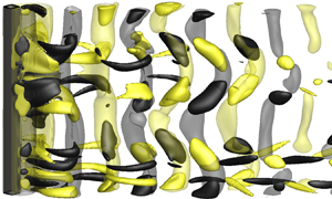A mesh convergence check was performed for the case L_z/h = 12 by increasing N_p from 5 to 6, where the St, $\overline {{C_D}}$ and ${C^{\prime}_L}$ values vary by less than 1%. It is seen in table 2 that with increasing L_z/h from 3 to 6, the wake structure changes from the ordered subharmonic mode (figure 20a) to disordered mode B (figure 20b). The existence of mode B rather than the subharmonic mode for L_z/h = 6 and 12 is supported by the following evidence.

1. (i) The streamwise vortices possess the spatio-temporal symmetry corresponding to mode B rather than the subharmonic mode.

2. (ii) The time-averaged lift coefficient is practically zero (of the order of 10⁻⁴).

3. (iii) The mode B structures emerge at Re ≥ 150, which is much smaller than the onset of the subharmonic mode at Re ~ 285.

Figure 20. Instantaneous vorticity fields for Re = 300 predicted by the 3-D DNS using (a) L_z/h = 3 and (b) L_z/h = 6. The translucent iso-surfaces represent spanwise vortices with ω_z = ±2, while the opaque iso-surfaces represent streamwise vortices with ω_x = ±0.4 for panel (a) and ω_x = ±2 for panel (b). Dark grey and light yellow denote positive and negative vorticity values, respectively. The flow is from left to right past the cylinder on the left.

Table 2. Wake structures for Re = 300 predicted by the 3-D DNS under different L_z/h constraints.

The development of mode B rather than the subharmonic mode in the natural 3-D flow is attributed to the influence of the mode A instability. The mode A streamwise vortices may destabilise mode B through (i) destabilising the braid shear layer region (Jiang et al. Reference Jiang, Cheng, Draper, An and Tong2016) for the hyperbolic instability of mode B (Williamson Reference Williamson1996; Leweke & Williamson Reference Leweke and Williamson1998; Thompson et al. Reference Thompson, Leweke and Williamson2001), and (ii) modulating the pattern of the spanwise vortices (i.e. the base flow) to allow for the instability of mode B. To demonstrate the latter mechanism, the span-averaged spanwise vorticity fields for Re = 300 computed with L_z/h = 3 and 6 are shown in figure 21. For L_z/h = 3, the ordered streamwise vortices of the subharmonic mode do not induce noticeable influence on the spanwise vortices (figure 20a), such that the pattern of the spanwise vortices shown in figure 21(a) is similar to that computed with 2-D DNS (figure 15a,b), where the primary vortex street transitions to the two-layered and secondary vortex streets at x/h ~ 4 and 10, respectively. For L_z/h = 6, the spanwise vortices are highly disordered (figure 20b), such that the spanwise vorticity field shown in figure 21(b) is based on a phase average over 25 vortex shedding cycles. Compared with figure 21(a), the pattern and strength of the spanwise vortices shown in figure 21(b) are significantly modulated by the disordered streamwise vortices (figure 20b) and the associated development of turbulence and turbulent dissipation.

Figure 21. Span-averaged spanwise vorticity fields for Re = 300, obtained from (a) the instantaneous 3-D flow field shown in figure 20(a) computed with L_z/h = 3, and (b) the phase-averaged 3-D flow computed with L_z/h = 6.

It is anticipated that the modulated pattern of the spanwise vortices may give rise to the instability of mode B. Therefore, an additional Floquet analysis is conducted, where the base flow is the phase- and span-averaged spanwise vorticity fields for Re = 300 obtained with L_z/h = 6 (called the modulated base flow hereafter). Figure 22 shows the |μ|−β relationship for Re = 300, predicted through the Floquet analysis using the modulated base flow. The two unstable modes identified in figure 22 both contain real and positive μ values, which correspond to synchronous modes. The streamwise perturbation vorticity fields for the two modes are shown in figure 23(a,b). The perturbation patterns of the two modes agree well with those for modes A and B for circular and square cylinders (see e.g. Robichaux et al. Reference Robichaux, Balachandar and Vanka1999; Carmo, Meneghini & Sherwin Reference Carmo, Meneghini and Sherwin2010). The most unstable spanwise wavelength for mode B (~0.9h) is similar to the wavelengths for mode B for circular and square cylinders (Barkley & Henderson Reference Barkley and Henderson1996; Choi et al. Reference Choi, Jang and Yang2012; Park & Yang Reference Park and Yang2016).

Figure 22. The |μ|−β relationship for Re = 300, predicted through the Floquet analysis using the modulated base flow. The horizontal dashed line marks the neutral instability of |μ| = 1.0.

Figure 23. Streamwise perturbation vorticity fields for Re = 300: (a) mode A predicted by βh = 1.8 of the modulated base flow, (b) mode B predicted by βh = 7 of the modulated base flow, (c) mode A predicted by βh = 1.4 of the phase-averaged base flow and (d) the subharmonic mode predicted by βh = 3.2 of the phase-averaged base flow. Red and blue denote positive and negative vorticity values, respectively.

For completeness, figure 23(c,d) shows the streamwise perturbation vorticity fields for mode A and the subharmonic mode predicted with the phase-averaged base flow illustrated in figure 17(a,b). For mode A, the perturbation structure displays opposite signs for the two sides of the wake centreline (figure 23a,c). For the subharmonic mode, the perturbation structure displays both signs alternately at each side of the wake centreline (figure 23d). The most unstable spanwise wavelength for the subharmonic mode (~1.9h) is similar to the wavelengths for the subharmonic mode observed in the wake of other bluff bodies (e.g. Sheard et al. Reference Sheard, Fitzgerald and Ryan2009; Yildirim, Rindt & van Steenhoven Reference Yildirim, Rindt and van Steenhoven2013).

However, figure 22 shows that the subharmonic mode is suppressed by the modulated pattern of the spanwise vortices shown in figure 21(b). As discussed earlier in this section, the subharmonic mode is unstable to the original and phase-averaged base flows where the spatio-temporal symmetry described in (3.5) is broken by the transition to the secondary vortex street relatively close to the cylinder. For the modulated base flow shown in figure 21(b), the two-layered vortices with significantly weakened vorticity do not transition to the secondary vortex street, and the wake possesses the spatio-temporal symmetry (see e.g. the $|{\overline {{C_L}} } |$ values in table 2), such that the subharmonic mode is suppressed.