


1. Introduction
Recently, scientists have taken a keen interest in the motion of microorganisms swimming in complex fluids (Spagnolie Reference Spagnolie2015; Patteson, Gopinath & Arratia Reference Patteson, Gopinath and Arratia2016). Examples of microscopic ‘swimmers’ moving through complicated biofluids abound: spermatozoa swims through the cervical mucus of the reproductive tract (Fauci & Dillon Reference Fauci and Dillon2006; Suarez & Pacey Reference Suarez and Pacey2006; Katz, Mills & Pritchett Reference Katz, Mills and Pritchett2008), the bacteria Escherichia coli resides in the mucus of the intestine (Sillankorva, Oliveira & Azeredo Reference Sillankorva, Oliveira and Azeredo2012) and Borrelia burgdorferi (the organism responsible for causing Lyme disease) must traverse the extracellular matrix of mammalian skin (Harman etal. Reference Harman, Dunham-Ems, Caimano, Belperron, Bockenstedt, Fu, Radolf and Wolgemuth2012). In each of these cases, the fluid in which the microorganism is immersed exhibits non-Newtonian behaviour due to the presence of large biological molecules creating a rich underlying microstructure (Spagnolie Reference Spagnolie2015). Understanding motility in these environments is not only interesting from a scientific perspective, but may also aid researchers in a variety of engineering applications, including preventing the spread of disease by disrupting biofilm formation (Costerton, Stewart & Greenberg Reference Costerton, Stewart and Greenberg1999). A fundamental understanding of how microorganisms propel in complex fluids also enables the development of more advanced synthetic swimmers, which have been designed for targeted drug delivery (Patra etal. Reference Patra, Sengupta, Duan, Zhang, Pavlick and Sen2013; Gao & Wang Reference Gao and Wang2014), minimally invasive surgery (Yan etal. Reference Yan, Zhou, Vincent, Deng, Yu, Xu, Xu, Tang, Bian and Wang2017) and various other biomedical applications (Li etal. Reference Li, De Ávila, Gao, Zhang and Wang2017).
It is now known that elasticity can impact the ability of an organism to swim, but this varies greatly depending on the kinematics of the gait (Godínez etal. Reference Godínez, Koens, Montenegro-Johnson, Zenit and Lauga2015; Elfring & Goyal Reference Elfring and Goyal2016), the structural properties of the immersed body and the rheology of the surrounding fluid (Dasgupta etal. Reference Dasgupta, Liu, Fu, Berhanu, Breuer, Powers and Kudrolli2013). In many cases, it has been observed that fluid elasticity can lead to a decrease in the swimming speed (Fu, Powers & Wolgemuth Reference Fu, Powers and Wolgemuth2007; Lauga Reference Lauga2007; Fu, Wolgemuth & Powers Reference Fu, Wolgemuth and Powers2009; Shen & Arratia Reference Shen and Arratia2011; Zhu etal. Reference Zhu, Do-Quang, Lauga and Brandt2011; Zhu, Lauga & Brandt Reference Zhu, Lauga and Brandt2012; Binagia, Guido & Shaqfeh Reference Binagia, Guido and Shaqfeh2019). One may then ask under what conditions can elasticity actually enhance the speed of a swimming microorganism? Several mechanisms for viscoelastic speed enhancement have been put forth, beginning with Teran, Fauci & Shelley (Reference Teran, Fauci and Shelley2010), who showed that large-amplitude undulatory motion could lead to a speed increase. Shortly thereafter, Liu, Powers & Breuer (Reference Liu, Powers and Breuer2011) and Spagnolie, Liu & Powers (Reference Spagnolie, Liu and Powers2013) found that large-amplitude motion was also required to observe a speed enhancement for the case of helical motion. Thomases etal. and Riley etal. later demonstrated the importance of the elasticity of the immersed body, finding that microorganisms with sufficiently flexibility would swim faster in viscoelastic fluids (Riley & Lauga Reference Riley and Lauga2014; Thomases & Guy Reference Thomases and Guy2014, Reference Thomases and Guy2017). Lastly, phase separation resulting from the depletion of polymer molecules near bacterial flagellum creates an apparent slip that allows microorganisms to swim faster in shear-thinning fluids (Martinez etal. Reference Martinez, Schwarz-Linek, Reufer, Wilson, Morozov and Poon2014; Man & Lauga Reference Man and Lauga2015; Zöttl & Yeomans Reference Zöttl and Yeomans2019).
In this report we propose an alternative mechanism for the speed enhancement of swimming microorganisms that originates from the coupling of fluid elasticity and local swirling flow. Indeed, previous studies have demonstrated that rotational motion can engender net translational motion in a viscoelastic fluid via hoop stresses that are created by the stretching of polymer molecules around the immersed body (Pak etal. Reference Pak, Zhu, Brandt and Lauga2012; Rogowski etal. Reference Rogowski, Kim, Zhang and JunKim2018; Puente-Velázquez etal. Reference Puente-Velázquez, Godínez, Lauga and Zenit2019). To date, however, no one has explicitly considered how this rotational–translational coupling may affect the propulsion of self-propelled swimming microorganisms. Certainly, it is not immediately clear what the effect will be; while the aforementioned studies consider a synthetic swimmer driven to rotate by an applied torque (created for example by a rotating magnetic field), swimming microorganisms are wholly self-propelled, capable of swimming in the absence of any external forces/torques. In studying this phenomenon, we are particularly motivated by recent experimental work studying the motion of E. coli in a viscoelastic fluid (Patteson etal. Reference Patteson, Gopinath, Goulian and Arratia2015). There, it was hypothesized that the increase in speed as a function of polymer concentration that was observed (Patteson etal. Reference Patteson, Gopinath and Arratia2016) might be a result of normal stress differences that could decrease cell ‘wobbling’ and create straighter and longer swimming trajectories. In this study we use a combination of numerical simulations and asymptotic theory to show that even a microswimmer constrained to swim in a straight line will experience a speed enhancement in a viscoelastic fluid so long as there is sufficient azimuthal swirl in its gait.
2. Mathematical model
2.1. The squirmer model
We first introduce the squirmer model (Lighthill Reference Lighthill1952; Blake Reference Blake1971), which is a spherical microscopic swimmer with a prescribed gait (given as a slip velocity at its surface). Thismodel has been widely used in the area of biological fluid mechanics to better understand the hydrodynamics of swimming microorganisms (Pedley Reference Pedley2016). It has especially been used to examine the effect that complex fluid rheology has on the swimming dynamics (Lauga Reference Lauga2009; Zhu etal. Reference Zhu, Do-Quang, Lauga and Brandt2011; Zhu, Lauga & Brandt Reference Zhu, Lauga and Brandt2012; Li, Karimi & Ardekani Reference Li, Karimi and Ardekani2014; Datt etal. Reference Datt, Zhu, Elfring and Pak2015, Reference Datt, Natale, Hatzikiriakos and Elfring2017; De Corato etal. Reference De Corato, Greco and Maffettone2015; Datt & Elfring Reference Datt and Elfring2019; Pietrzyk etal. Reference Pietrzyk, Nganguia, Datt, Zhu, Elfring and Pak2019). The general slip velocity for a steady axisymmetric squirmer exhibiting purely tangential deformations is given by Pak & Lauga as (Pak & Lauga Reference Pak and Lauga2014)
 \begin{equation} \boldsymbol{{{u}}}^{\boldsymbol{{{s}}}}(\theta,\phi)= \sin(\theta)\left\{\sum_{n=1}^\infty \frac{2P'_n}{(n+1)n}B_n \boldsymbol{{{e}}}_{\theta} + \sum_{n=1}^\infty \frac{P'_n}{a^{n+1}}C_n \boldsymbol{{{e}}}_{\phi}\right\}, \end{equation}
where  $a$ is the squirmer's radius,
  $\theta$ is the polar angle (
 $0\le \theta \le \pi$) and
  $\phi$ is the azimuthal angle (
 $0\le \phi <2\pi$);
  $P_n'(\mu )$ is the first derivative of the Legendre polynomial of degree
  $n$, where
  $\mu =\cos (\theta )$. The polar and azimuthal squirming modes are given by
  $B_n$ and
  $C_n$, and
  $\boldsymbol{e}_{\theta}$ and
  $\boldsymbol{e}_{\phi}$ are the unit vectors in the polar and azimuthal directions, respectively.
Typically, authors only consider the first two polar squirming modes, those related to the coefficients  $B_1$ and
  $B_2$ in (2.1). This is usually done because in a Newtonian fluid the swimming speed is determined solely by the value of
  $B_1$, i.e.
  $U_N=\frac {2}{3} B_1$ (Lighthill Reference Lighthill1952; Blake Reference Blake1971), while
  $B_2$ is the only coefficient appearing in the particle stresslet (Ishikawa, Simmonds & Pedley Reference Ishikawa, Simmonds and Pedley2006). Furthermore, these are the only two modes necessary to differentiate between pushers, i.e. swimmers who generate thrust from behind their body (e.g. E. coli) and pullers, swimmers who generate thrust from the front of their body (e.g. Chlamydomonas reinhardtii). Only recently have authors started to consider the effect of higher-order polar squirming modes (Datt etal. Reference Datt, Zhu, Elfring and Pak2015; De Corato & D'Avino Reference De Corato and D'Avino2017; Pietrzyk etal. Reference Pietrzyk, Nganguia, Datt, Zhu, Elfring and Pak2019) or the azimuthal squirming modes (Ghose & Adhikari Reference Ghose and Adhikari2014; Pak & Lauga Reference Pak and Lauga2014; Felderhof & Jones Reference Felderhof and Jones2016; Pedley Reference Pedley2016; Pedley, Brumley & Goldstein Reference Pedley, Brumley and Goldstein2016). To date, however, no one has considered how the presence of the azimuthal modes of the squirmer model impacts swimming kinematics in a complex fluid.
2.2. Governing equations
We proceed by considering the flow generated by the swimming microorganism, which must obey conservation of momentum and the continuity equation. In dimensionless form these equations are given by
 \begin{equation} {Re} \left(\frac{\partial\boldsymbol{{{u}}}}{\partial t} + \boldsymbol{{{u}}}\boldsymbol{\cdot} \boldsymbol{\nabla}\boldsymbol{{{u}}} \right)= \boldsymbol{\nabla}\boldsymbol{\cdot} \boldsymbol{\sigma}, \quad \boldsymbol{\nabla}\boldsymbol{\cdot}\boldsymbol{{{u}}}=0,\end{equation}
where  $\boldsymbol {{{u}}}$ is the fluid velocity,
  $p$ is pressure and
  $\boldsymbol {\sigma }$ is the Cauchy stress tensor. We have scaled velocities with the first swimming mode
  $B_1$, lengths with the squirmer radius
  $a$, time with the convective time scale
  $a/B_1$ and stresses with
  $\mu _0 B_1/a$, where
  $\mu _0$ is the total zero-shear viscosity of the fluid. The Reynolds number is given by
  ${Re}=\rho B_1 a/\mu _0$ where
  $\rho$ is the fluid density. Owing to their small size and the viscous environments in which they are commonly found, microorganisms swim at virtually zero Reynolds number (Purcell Reference Purcell1977). Thus, we assume Stokes flow (
 ${Re}= 0$) for our asymptotic theory, and conduct our numerical simulations at sufficiently low
  $Re$ such that the kinematics are not significantly affected by inertia; we find
  ${Re} = 0.1$ to be sufficient for these purposes.
For a viscoelastic fluid, the total stress  $\boldsymbol {\sigma }$ can be expressed as
 \begin{equation} \boldsymbol{\sigma} = -p\boldsymbol{{{I}}} + \beta(\boldsymbol{\nabla}\boldsymbol{{{u}}} + \boldsymbol{\nabla}\boldsymbol{{{u}}}^T) + \boldsymbol{\tau}^p, \end{equation}
where  $\boldsymbol{\tau }^p$ is the polymer extra-stress tensor and
  $\beta =\mu _s/(\mu _s + \mu _p)=\mu _s/\mu _0$ is the viscosity ratio for a fluid with solvent viscosity
  $\mu _s$ and polymer viscosity
  $\mu _p$;
  $\boldsymbol{\tau }^p$ is determined with the Giesekus constitutive model (Giesekus Reference Giesekus1982)
 \begin{gather} \boldsymbol{\tau}^{p} = \frac{1-\beta}{{Wi}}(\boldsymbol{{{c}}}-\boldsymbol{{{I}}}) \end{gather}
 \begin{gather} {Wi} \stackrel{\triangledown}{\boldsymbol{{{c}}}} +\ (\boldsymbol{{{c}}}-\boldsymbol{{{I}}}) +\alpha_m(\boldsymbol{{{c}}}-\boldsymbol{{{I}}})^2 = 0. \end{gather}
In (2.4) and (2.5),  $\boldsymbol {{{c}}}$ is the polymer conformation tensor,
  $\stackrel {\triangledown }{\boldsymbol {{{c}}}}\ =\ \partial \boldsymbol {{{c}}}/\partial t+\boldsymbol {{{u}}}\boldsymbol {\cdot }\boldsymbol {\boldsymbol{\nabla} } \boldsymbol {{{c}}}-\boldsymbol {\boldsymbol{\nabla} } \boldsymbol {{{u}}}^T\boldsymbol {\cdot } \boldsymbol {{{c}}}-\boldsymbol {{{c}}} \boldsymbol {\cdot }\boldsymbol {\boldsymbol{\nabla} } \boldsymbol {{{u}}}$ is the upper-convected time derivative, and
  ${Wi} = \lambda B_1/a$ is the Weissenberg number, which describes the degree of fluid elasticity. The Giesekus constitutive equation considers the polymer molecules in the fluid to be Hookean dumbbells, and allows for anisotropic drag on these dumbbells via the Giesekus mobility parameter
  $\alpha _m$ (Bird, Armstrong & Hassager Reference Bird, Armstrong and Hassager1977).
3. Solution methodology
3.1. Numerical solution
We numerically solve the above set of equations as follows. We consider the co-moving frame of reference, i.e. the stationary squirmer experiences a uniform flow given by  $-U\boldsymbol {{{e}}}_{\boldsymbol {{{z}}}}$. This uniform flow is imposed on the outer walls of a cylindrical domain with length
  $40a$ and radius 20
 $a$. This simulation set-up is shown in figure 1(a). This uniform flow is also specified at the inlet (top) of the box, where additionally the conformation tensor is set to identity,
  $\boldsymbol {{{c}}}=\boldsymbol {{{I}}}$. A convective outlet boundary condition is used at the exit of the simulation box.

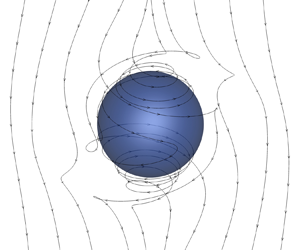
Figure 1. (a) Simulation set-up for a squirmer with swirl as seen in the co-moving frame (swimming in the positive  $z$ direction). Note that the dimensions are not drawn to scale. (b)Streamlines around the neutral squirmer (
 $\xi$) at
  ${Wi} = 0$ and
  $\zeta =5$, shown to illustrate the qualitative shape of the flow that results from the inclusion of the term related to azimuthal swirl in (3.1).
As a minimal model for a squirmer with swirl, we consider the slip velocity given by (2.1) with the first two polar modes (corresponding to  $B_1$ and
  $B_2$) and the second azimuthal mode (corresponding to
  $C_2$) as being non-zero. Thus, in the chosen frame of reference, the boundary condition at the surface of the squirmer is
 \begin{equation} \boldsymbol{{{u}}}|_{r=1} = \left(\sin(\theta) + \frac{\xi}{2}\sin(2\theta)\right) \boldsymbol{{{e}}}_{\theta} +\left(\Omega \sin(\theta) + \frac{3\zeta}{2}\sin(2\theta)\right)\boldsymbol{{{e}}}_{\phi}. \end{equation}
As previously discussed,  $\xi =B_2/B_1$ denotes the type of swimmer: pushers have
  $\xi <0$, pullers have
  $\xi >0$ and ‘neutral’ squirmers have
  $\xi =0$. The new dimensionless group
  $\zeta =C_2/(B_1 a^3)$ denotes the relative magnitude of the azimuthal to the polar flow around the swimming organism. The reason we consider the
  $C_2$ swirling mode, corresponding to a rotlet dipole flow (Pak & Lauga Reference Pak and Lauga2014), is to produce in a simple way the flow field of a microorganism with a rotating flagellum and counter-rotating body. To illustrate this flow qualitatively, in figure 1(b), we visualize streamlines around a neutral squirmer (
 $\xi =0$) for
  $\zeta =5$ and
  ${Wi}=0$.
We solve the above governing equations and boundary conditions using a third-order accurate finite volume flow solver developed by Stanford's Center for Turbulence Research (Ham, Mattsson & Iaccarino Reference Ham, Mattsson and Iaccarino2006). Equation (2.5) is solved as six scalar equations (since  $\boldsymbol {{{c}}}$ is symmetric) using a log-conformation approach to ensure
  $\boldsymbol {{{c}}}$ remains positive–definite (Fattal & Kupferman Reference Fattal and Kupferman2004; Hulsen, Fattal & Kupferman Reference Hulsen, Fattal and Kupferman2005). Further details of the method described thus far, including extensive validation studies and comparison with experiments, can be found in previously published works (Richter, Iaccarino & Shaqfeh Reference Richter, Iaccarino and Shaqfeh2010; Padhy etal. Reference Padhy, Shaqfeh, Iaccarino, Morris and Tonmukayakul2013; Yang, Krishnan & Shaqfeh Reference Yang, Krishnan and Shaqfeh2016; Castillo etal. Reference Castillo, Murch, Einarsson, Mena, Shaqfeh and Zenit2019). Since a microorganism swimming at low Reynolds number must be force and torque free (Lauga & Powers Reference Lauga and Powers2009), we iteratively calculate
  $U$ and
  $\Omega$ through time stepping until the
  $z$-components of the measured net force and torque on the squirmer vanish at steady state (the other components of force and torque vanish due to the axisymmetry of the problem). Since we work in the co-moving frame of reference, it is natural to use a body-fitted mesh; thus we make use of an unstructured mesh of tetrahedral elements with increasing resolution near the squirmer. We have conducted a series of studies on successively refined meshes in space and time to ensure the accuracy of our simulations; the kinematic results presented change by no more than 1 % when moving to a mesh size or time step size that is two times as coarse.
3.2. Asymptotic solution
We augment our simulations with an asymptotic theory valid in the limit of  ${Wi} \ll 1$. Specifically, we consider a regular perturbation expansion to obtain
  $U$ and
  $\Omega$ as a power series in Wi. The theoretical analysis is performed using (2.2), (2.3) and (2.5) for zero Reynolds numbers (
 $Re = 0$), an unbounded flow, and assuming steady state. Because of the particle geometry, the equations are expressed conveniently in a spherical coordinate system
  $r\theta \phi$ where
  $r$ is the distance from the centre of the particle,
  $\theta$ is the polar angle (
 $0\le \theta \le \pi$) and
  $\phi$ is the azimuthal angle (
 $0\le \phi <2\pi$). The domain of definition of the governing equations is
  $\boldsymbol {{{D}}} =\{1<r<\infty,\, 0<\theta <\pi,\, 0\le \phi <2\pi \}$. Although all the components of the velocity are non-zero, the flow is axisymmetric, i.e. there is no dependence of the dependent flow variables on
  $\phi$:
 \begin{align} p=p(r,\theta ),\enspace \boldsymbol{{{u}}}=\sum _{i=r,\theta,\phi } u_{i} (r, \theta )\, \boldsymbol{{{e}}}_{i},\enspace \boldsymbol{\tau}^p=\sum _{i,j=r,\theta,\phi } \tau _{i,j}^{{p}} (r, \theta )\, \boldsymbol{{{e}}}_{i} \boldsymbol{{{e}}}_{j},\enspace \boldsymbol{{{c}}}=\sum _{i,j=r,\theta,\phi }c_{i,j} (r, \theta )\, \boldsymbol{{{e}}}_{i} \boldsymbol{{{e}}}_{j}. \end{align}
Note that  $\boldsymbol{\tau }^p$ and
  $\boldsymbol {{{c}}}$ are connected linearly (see (2.4) above). In the spherical coordinate system, the boundary conditions on the surface of the particle are
 \begin{equation} u_r =0,\quad u_{\theta} =\sin (\theta )+\frac{\xi }{2} \sin (2\theta ),\quad u_{\phi} =\Omega \sin (\theta )+\frac{3}{2}\zeta \sin (2\theta )\quad \textrm{at}\ r=1. \end{equation}
The above conditions in conjunction with the continuity equation give
 \begin{equation} \left. \frac{\partial u_r }{\partial r} \right|_{r=1} =-\frac{\xi }{2} -2\cos (\theta )-\frac{3\xi }{2} \cos (2\theta ). \end{equation}
Far from the particle, the far-field flow is given as
 \begin{equation} u_r^{\infty } =-U\cos (\theta ),\quad u_{\theta}^{\infty } =U\sin (\theta ),\quad u_{\phi}^{\infty } =0,\quad p^{\infty } =0, \end{equation}
where the superscript  $\infty$ denotes value at infinity (
 $r\to \infty$).
The unknown far-field flow velocity,  $U$, and rotation rate of the particle,
  $\Omega$, are determined by ensuring the microswimmer is force and torque free (Lauga & Powers Reference Lauga and Powers2009)
 \begin{equation} \int_{r=1} \boldsymbol{{{e}}}_{r} \boldsymbol{\cdot} \boldsymbol{\sigma} \,\textrm{d}S = \textbf{{0}}, \quad \int_{r=1} \boldsymbol{{{e}}}_{r}\times (\boldsymbol{{{e}}}_{r} \boldsymbol{\cdot} \boldsymbol{\sigma}) \,\textrm{d}S = \textbf{{0}}. \end{equation}
The non-trivial components of the force-free condition (FFC) and the torque-free condition (TFC) are, respectively,
 \begin{align} & \int _{0}^{\pi }\left\{\left(\frac{p}{2} \sin (2\theta )\right)+\beta \left(\left(\frac{1}{r}\frac{\partial u_r}{\partial\theta}+\frac{\partial u_{\theta} }{\partial r} -\frac{u_{\theta}}{r} \right)\sin ^{2} (\theta )-\frac{\partial u_r }{\partial r} \sin (2\theta )\right)\right.\nonumber\\ &\left.\quad +\left(\tau _{r\theta }^{p} \sin ^{2} (\theta )-\tau _{rr}^{p} \frac{\sin (2\theta )}{2} \right)\right\}\textrm{d}\theta =0 \end{align}
 \begin{equation} \int _{0}^{\pi }\left(\beta \left(\frac{\partial u_{\phi} }{\partial r} -\frac{u_{\phi}}{r} \right)+\tau _{r\phi }^{p} \right)\sin ^{2} (\theta )\,\textrm{d}\theta =0. \end{equation}
Although (3.7) and (3.8) are evaluated at  $r=1$ in order to determine
  $U$ and
  $\Omega$, one can prove that, under steady state and creeping conditions, they hold at any radial position,
  $r\ge 1$. Finally, note that with the asymptotic analysis, no boundary conditions are applied (and cannot be imposed) for the polymer extra stress
  $\boldsymbol{\tau }^p$.
In order to solve (2.2), (2.3) and (2.5) accompanied by the auxiliary conditions ((3.3) to (3.5) and (3.8) and § 3.2), we use a regular perturbation scheme in terms of the Weissenberg number. In particular, for a weakly viscoelastic fluid, i.e.  $0<{Wi}<<1$, the solution for all the dependent variables is given as a standard power series expansion in terms of
  ${Wi}$
 \begin{equation} \left. \begin{array}{@{}c@{}} {X\approx X_{0} +{Wi}\, X_{1} +{Wi}^{2} \, X_{2} +\cdots}\\ {X=U,\Omega,p,u_r,u_{\theta},u_{\phi},\tau^p _{rr},\tau^p _{\theta \theta },\tau^p _{r\theta },\tau^p _{\phi \phi },\tau^p _{r\phi },\tau^p _{\theta \phi } }\end{array}\right\}, \end{equation}
where the zero-order term,  $X_{0}$, corresponds to the simple Newtonian fluid. In this type of analysis, the remaining parameters
  $a_{m},\beta,\zeta,\xi$ are considered
  $O(1)$ quantities. The solution procedure for a similar flow problem with no-slip boundary conditions has been described in recent work by Housiadas (Reference Housiadas2019) and the interested reader is referred thereto for more details.
The analytical solution for the Newtonian fluid, i.e. for the Stokes equations, is
 \begin{gather} u_{r,0} =\frac{\xi }{4} \left(\frac{1}{r^{4} } -\frac{1}{r^{2} } \right)\left(1+3\cos (2\theta )\right)+U_0 \left(\frac{1}{r^{3} } -1\right)\cos (\theta ), \end{gather}
 \begin{gather}u_{\theta,0} =U_0\left(1+\frac{1}{2r^{3} } \right)\sin (\theta )+\frac{\xi }{2r^{4} } \sin (2\theta ), \end{gather}
 \begin{gather}u_{\phi,0} =\frac{\Omega _{0} }{r^{2} } \sin (\theta )+\frac{3\zeta }{2r^{3} } \sin (2\theta ), \end{gather}
 \begin{gather}p_{0} =-\frac{\xi }{2r^{3} } \left(1+3\cos (2\theta )\right). \end{gather}
Note that  $U_{0} =\frac {2}{3}$ and
  $\Omega _{0} =0$ have been determined. We have also solved the perturbation equations analytically up to
  $O({Wi}^{4})$ using the ‘Mathematica’ software (Wolfram Research, Inc. 2019). The most important results are the velocity at infinity and the rotation rate of the swimmer. We find
 \begin{equation} U\approx \frac{2}{3} +(1-\beta )\, {Wi} \left(U_{1} + {Wi}\, U_{2} + {Wi}^{2} \, U_{3} + {Wi}^{3} \, U_{4} \right), \end{equation}
where  $U_{1}$ and
  $U_{2}$, respectively, are
 \begin{equation} U_{1} = \frac{2}{15}(\alpha_m - 1)\xi \end{equation}
 \begin{align} U_{2} &=\left(-\frac{772}{2145} -\frac{64\alpha_m}{65} +\frac{128\alpha_{m}^{2} }{195} \right) \nonumber\\ &\quad +\xi ^{2} \left(-\frac{6218}{15015} -\frac{101168a_{m} }{45045} +\frac{7376a_{m}^{2} }{5005} +\left(-\frac{58}{1365} +\frac{3032a_{m} }{45045} -\frac{86a_{m}^{2} }{3465} \right)(1-\beta )\right) \nonumber\\ &\quad +\zeta ^{2} \left(\frac{468}{385} -\frac{21744\alpha_m }{5005} +\frac{15744a_{m}^{2} }{5005} +\left(-\frac{4392}{5005} +\frac{1944a_{m} }{1001} -\frac{5328a_{m}^{2} }{5005} \right)(1-\beta )\right). \end{align}
For the rotation rate of the particle, we have found the solution up to fifth order in Wi
 \begin{equation} \Omega \approx \zeta\, {Wi} (1-\beta) \left(\Omega _{1} +{Wi}\, \Omega _{2} +{Wi}^{2} \, \Omega _{3} +{Wi}^{3} \, \Omega _{4} +{Wi}^{4} \, \Omega _{5} \right), \end{equation}
where  $\Omega _{1}$ and
  $\Omega _{2}$ are given below.
 \begin{gather} \Omega _{1} = \frac{6}{5}(1-\alpha_m), \end{gather}
 \begin{gather} \Omega_2 = \xi\frac{12(1043+2912\alpha_m-2000\alpha_m^2)-6(623-1158\alpha_m+535\alpha_m^2)(1-\beta)}{5005}. \end{gather}
The higher-order corrections for  $U$ and
  $\Omega$ are available upon request. Note that setting
  $\zeta =0$ and
  $\beta =0$ recovers the solution of Datt & Elfring (Reference Datt and Elfring2019, Reference Datt and Elfring2020) through
  $O({Wi}^3)$.
4. Results and discussion
4.1. The effect of azimuthal swirl on the swimming speed
We begin by looking at the effect of azimuthal swirl on the kinematics of the swimmer. Note that, while the rotation rate for our particular swimming gait is zero in a Newtonian fluid and under creeping flow conditions ( $Re = 0$), i.e.
  $\boldsymbol {\Omega }_N= - C_1\boldsymbol {{{e}}}_{\boldsymbol {{{z}}}}/a^3$ as given by Pak& Lauga (Reference Pak and Lauga2014), it is actually non-zero but small (
 $\Omega \le 0.25$) for finite Wi due to the nonlinear coupling between rotation and translation in a viscoelastic fluid (Castillo etal. Reference Castillo, Murch, Einarsson, Mena, Shaqfeh and Zenit2019). Interestingly enough, the effect of this coupling on rotation rate even vanishes in the presence of significant fluid elasticity. We illustrate this in figure 2(b), where we plot the rotation rate scaled by its dominant scaling (as found in the previous section) for the case of a neutral squirmer. From this plot we see that there will only be a slight rotation due to the azimuthal swirl solely for small but finite Wi (i.e.
  $0.1 \lessapprox {Wi} \lessapprox 1$). Because of this, we will focus our attention on the change in translational speed for the remainder of this report. Unless otherwise stated, we will consider
  $\beta =0.5$ and
  $\alpha _m=0.2$ for the rheological properties of the fluid.

Figure 2. (a) Normalized swimming speed ( $U/U_N$) and (b) scaled rotation rate as a function of Wi and
  $\zeta$ for the neutral squirmer (
 $\xi =0$). Filled circles refer to numerical simulations while dashed lines refer to the asymptotic theory through
  $O({Wi}^2)$ for
  $U$ and through
  $O({Wi}^3)$ for
  $\Omega$. The results are presented in this way since only even (odd) terms with respect to Wi are non-zero in the asymptotic expansion for
  $U$ (
$U$ ( $\Omega$) for the neutral squirmer. For significant swirl (
 $\zeta = 3, 5)$, the squirmer swims faster in the viscoelastic fluid, with the speed increase growing with increasing fluid elasticity (Wi).
We first recall the effect of elasticity for the case of no swirl, where it was found that squirmers swim slower in a viscoelastic fluid for all Wi (Zhu etal. Reference Zhu, Do-Quang, Lauga and Brandt2011, Reference Zhu, Lauga and Brandt2012). This result corresponds to the case of  $\zeta =0$ in figure 2, where we plot the swimming speed of the neutral squirmer (
 $\xi = 0$) normalized by the Newtonian swimming speed
  $U_N$ as a function of Wi and
  $\zeta$. Our results for
  $\zeta =0$ differ by no more than 2.8 % from those of Zhu etal. (Reference Zhu, Lauga and Brandt2012), serving as one validation of our current results. Without loss of generality we consider only positive
  $\zeta$ since changing its sign does not alter its effect on
  $U$ from symmetry. For the cases of zero (
 $\zeta =0$) or relatively small (
 $\zeta =1$) azimuthal swirl we see that the squirmer swims slower in a viscoelastic fluid than it does in a Newtonian fluid. In stark contrast, for significant swirling flow (
 $\zeta = 3, 5$), the normalized speed exceeds unity indicating speed enhancement. Increasing Wi causes the effect to become more pronounced before appearing to reach an asymptotic value at large Wi. For all values of
  $\zeta$, our numerical results are corroborated by the asymptotic theory (shown as dashed curves, cf. figures 2a and 3a) for small Wi, i.e. (3.14). The reason the agreement of the numerical solution with the asymptotic results is good only for small Wi is the strongly nonlinear character of the swirling slip velocity with viscoelasticity. It is also an indication of a coil–stretch transition at a finite Weissenberg number
  ${Wi}_c$, a case that does not allow for accurate predictions of the flow close to
  ${Wi}_c$ using high-order perturbations methods (Housiadas Reference Housiadas2017).

Figure 3. Normalized swimming speed ( $U/U_N$) as a function of Wi and
  $\zeta$ for the neutral squirmer (
 $\xi =0$). In (a) we recapitulate the results of figure 2(a) to better visualize the trends at low Wi. Dashed lines refer to the
  $O({Wi}^2)$ solutions. In (b) we examine how the results change in the presence and absence of inertia (
 $Re = 0.1$ and 0, respectively). The latter (
 $Re = 0$) results were obtained by solving (2.2) after discarding the nonlinear convective term.
As mentioned in § 2.1, we nominally perform our simulations at a  $Re$ small enough such that the effect of inertia is minimized. We have also performed an additional set of simulations whereby we solved (2.2) only after completely discarding the second term, which represents convective forces in the fluid. In this way, we can carefully examine the impact inertia has in regards to creating a speed enhancement. These simulations are shown for the case of a neutral squirmer with swirl (
 $\zeta =3, 5$) in figure 3(b). From this figure, we see that at most the error in retaining all terms of the Navier–Stokes equation is approximately 7 % (seen at the largest value of
  ${Wi} = 3$ and
  $\zeta =5$). For smaller
  $\zeta$, the difference is reduced to a few percentage points; indeed, one expects the difference in these two solution methodologies to vanish as
  $\zeta$ decreases since
  $\zeta$ controls the relative amount of rotational inertia in the fluid. An additional conclusion to be made from figure 3(b) is that the nonlinear rotational–translational coupling originating from fluid inertia (rather than fluid elasticity) appears to act synergistically with the latter to further increase the swimming speed. Since we are primarily interested in this work in the coupling originating from fluid elasticity rather than inertia, all subsequent simulations where we expect rotational inertia to be significant (i.e.
  $\zeta \ge 3$) are conducted at
  $Re = 0$ unless stated otherwise. In this way, our simulation results will present a lower bound on the effect of swirl in a viscoelastic fluid since any real swimming microorganism will experience some finite amount of inertia.
4.2. The relationship between speed enhancement and the polymer stress in the surrounding flow
To better understand the origin of the speed enhancement seen in figure 2, we examined the polymer stress field around the neutral squirmer in the case of no azimuthal swirl ( $\zeta = 0$) and a significant degree of swirl (
 $\zeta = 5$) in figure 4. In figure 4, we are viewing the
  $y=0$ plane for a swimmer moving in the positive
  $z$-direction. We first look at the z–z component of the polymer stress tensor, shown in figure 4(a) as a function of
  $\zeta$. It is seen that the large amount of extensional stress in the swimmer's wake in the case of no swirl diminishes dramatically in the presence of significant swirling flow. This follows since for no swirl the back of the swimmer is an extensional point in the flow field, where polymers can readily deform and cause marked decrease in swimming speeds (Shen & Arratia Reference Shen and Arratia2011; Binagia etal. Reference Binagia, Guido and Shaqfeh2019). By changing the slip velocity to include an azimuthal component, we necessarily introduce a vortical component to the flow near this location, thereby decreasing its extensional character. With the diminution of extensional stress, we see the creation of hoop stresses (corresponding to
  $\tau _{\phi \phi }^p$ in spherical coordinates) when azimuthal swirl is included in the model (cf. figure 4b). Note that this is the type of stress alluded to by Patteson etal. (Reference Patteson, Gopinath, Goulian and Arratia2015), who hypothesized that hoop stresses could decrease cell wobbling and thereby lead to straighter swimming trajectories and consequently faster speeds.

Figure 4. Components of the polymer stress tensor ( $\boldsymbol{\tau }^p$) surrounding the neutral squirmer (swimming in the positive
  $z$ direction) at
  ${Wi} = 2$. (a) The z–z component of the polymer stress (
 $\tau _{zz}^p$) is largest behind the swimmer and diminishes once swirl is introduced (
 $\zeta =5$). (b) In contrast, the
  $\phi$–
 $\phi$ component of the polymer stress (
 $\tau _{\phi \phi }^p$) is essentially non-existent in the case of no swirl (
 $\zeta =0$) and becomes the dominant component of the polymer stress tensor at
  $\zeta =5$.
These trends for the polymer stress suggest a possible mechanisms for the speed enhancement seen in figure 2. As the large extensional  $\tau _{zz}^p$ stress found behind the swimmer in the case of no swirl (
 $\zeta =0$) was previously reported to be responsible for speed hindrance (Zhu etal. Reference Zhu, Lauga and Brandt2012), we expect its diminution to lead to an increase in the swimming speed.
To examine this hypothesis in more detail we consider the force tractions acting on the surface of the swimming microorganism. The net force acting on the particle in the swimming direction is given in indicial notation by  $F_z = \int _S \sigma _{z\,j} n_j \,\textrm {d}S = 0$. This net force can be decomposed into pressure, viscous and polymeric contributions according to (2.3): i.e.
  $F_z = F_z^{pres} + F_z^{visc} + F_z^{poly} = 0$. We plot each of these contributions to the net force in figure 5 as a function of Wi for
  $\zeta = 0$ and
  $\zeta =5$. We also further decompose the polymer contribution into that related to the normal stress
  $\tau _{zz}^p$ and the shear stress
  $\tau _{z\rho }^p$ (where
  $\rho$ refers to the radial coordinate in cylindrical coordinates). That is,
  $F_z^{poly} = \int _S \tau ^p_{zz}n_z \,\textrm {d}S + \int _S \tau ^p_{z\rho }n_\rho \,\textrm {d}S$ (with no contribution related to
  $\tau _{z\phi }^p$ since
  $n_{\phi } = 0$). We see from figure 5 that the inclusion of azimuthal swirl (i.e. moving from figures 5a to 5b) only causes a slight change in the contribution related to the polymer shear stress
  $\tau ^p_{z\rho }$. In contrast, the presence of swirl significantly affects the normal stress (
 $\tau ^p_{zz}$) contribution to the net force, causing it to not only increase but actually become propulsive for all Wi. This trend can be anticipated from figure 4(a), where the inclusion of swirl removes the region of high extensional resistance behind the swimmer but does not significantly change the small regions located at the front half of the swimmer that yield positive contributions to the net force.

Figure 5. Net force contributions acting in the swimming ( $z$) direction in the case of (a)
 $\zeta =0$ and (b)
  $\zeta =5$. The pressure, viscous and polymer contributions are given in cylindrical coordinates by
  $F_z^{pres}=-\int _S p n_z \,\textrm {d}S$,
  $F_z^{visc}=\beta \int _S (\boldsymbol {\boldsymbol{\nabla} }_z u_j + \boldsymbol {\boldsymbol{\nabla} }_j u_z) n_j \,\textrm {d}S$ and
  $F^{poly}_z=\int _S \tau ^p_{zj}n_j\,\textrm {d}S$, respectively (i.e.
  $F_z = F_z^{pres} + F_z^{visc} + F_z^{poly} = 0$). The polymer stress contribution,
  $F^{poly}_z$, is further broken down into portions related to normal polymeric stresses (
 $\tau ^p_{zz}$) and shear polymeric stresses (
 $\tau ^p_{z\rho })$; notably, the former becomes positive (acting as a thrust) for all Wi in the presence of significant swirl (
 $\zeta =5$).
To better visualize this, in figure 6 we plot the surface tractions related to  $\tau ^p_{zz}$ and
  $\tau ^p_{z\rho }$ as a function of the polar angle
  $\theta$. We immediately see that the biggest change with the addition of swirl occurs at the back of the swimmer, i.e. near
  $\theta =\pi$. Notably,
  $\tau ^p_{zz}n_z$, which nominally is responsible for the slow down in the case of no swirl (Zhu etal. Reference Zhu, Lauga and Brandt2012), severely decreases in magnitude as
  $\zeta$ is increased. All else equal, one would expect this to lead to an increase in the swimming speed. Of course the net effect depends on how the surface tractions related to the hoop stresses, i.e.
  $\tau ^p_{z\rho }n_{\rho }$, vary with
  $\zeta$. From figure 6(b), we that while there is an increase of
  $\tau ^p_{z\rho }n_{\rho }$ for most values of
  $\theta$ in the presence of swirl, a significant decrease is seen near
  $\theta =\pi$. These two trends appear to offset each other; this explains the minimal change in the component of
  $F_z$ related to
  $\tau ^p_{z\rho }$ seen in figure 5. We thus argue that it is the change in the extensional stress that dominates the change in speed. Thus, taking the results of figures 4 to 6 together, we conclude that the microswimmer experiences an increase in its swimming speed when the rotational flow originating from the rotlet dipole squirming mode is significant enough to disrupt the predominantly extensional flow behind the squirmer.

Figure 6. Surface tractions (a)  $\tau ^p_{zz}n_z$ and (b)
  $\tau ^p_{z\rho }n_z$ as a function of the polar angle
  $\theta$ and the degree of azimuthal swirl,
  $\zeta$, for a neutral squirmer at
  ${Wi} = 2$. With increasing swirl,
  $\tau ^p_{zz}n_z$ degrees in magnitude near the back of the squirmer (
 $\theta =\pi$). In contrast,
  $\tau ^p_{z\rho }n_z$ increases with increasing
  $\zeta$ for most values of
  $\theta$, except near
  $\theta =\pi$ where it decreases significantly and actually changes sign.
4.3. The effect of the swimmer type ( $\xi$) and Giesekus mobility parameter ($\alpha _m$)


We would now like to examine how robust the results seen in figure 2 (namely the speed enhancement for significant azimuthal swirl) are to changes in the swimmer type and the degree of shear-thinning present in the viscoelastic fluid (tuned via the Giesekus mobility parameter  $\alpha _m$). In figure 7 we plot the normalized swimming speed for a pusher (
 $\xi =-1$), a puller (
 $\xi =1$), and a neutral squirmer (
 $\xi =0$) as a function of Wi at
  $\zeta = 5$. We see that the effect of swimming type is modest; pullers exhibit a slightly more pronounced speed enhancement than that of neutral squirmers while the effect is diminished for pushers. This makes sense in light of the results of Zhu etal. (Reference Zhu, Lauga and Brandt2012), where it was found that the pusher had the greatest region of extensional stress behind the swimmer by a large margin when compared with that of the other swimmer types. Given the mechanism we described in the preceding paragraph, we therefore expect the pusher to experience a smaller speed increase compared with the other swimmer types in the presence of significant swirl given that there is a greater degree of extensional resistance in the wake to overcome.

Figure 7. Normalized swimming speed ( $U/U_N$) as a function of fluid elasticity (Wi), swimmer type (
 $\xi$) and fluid rheology (
 $\alpha _m$) in the case of significant swirl (
 $\zeta = 5$). Filled circles refer to numerical simulations while dashed lines refer to the asymptotic theory through
  $O({Wi}^2)$.
In figure 7(b) we plot the normalized swimming speed for the neutral squirmer ( $\xi =0$) as a function of Wi and the Giesekus mobility parameter (
 $\alpha _m$). Note that, in the limit of
  $\alpha _m = 0$, the Oldroyd-B model is recovered, which does not exhibit shear thinning (Giesekus Reference Giesekus1982). Thus, decreasing
  $\alpha _m$ amounts to systematically removing shear thinning from the predictions of the constitutive model for pure shearing. Interestingly, we see from figure 7(b) that the speed enhancement seen in figure 2 for
  $\alpha _m = 0.2$ actually becomes more pronounced as
  $\alpha _m$ is decreased for all but the largest value of
  ${Wi}=3$. We explore this effect further in figure 8, where we examine the swimming speed for a neutral squirmer with significant swirl (
 $\xi =0$,
  $\zeta =5$) at
  ${Wi} = 0.5$ as a function of
  $\alpha _m$. We see that as
  $\alpha _m$ approaches zero, both theory (specifically, the diagonal Padé [2/2] approximant of (3.14); Housiadas Reference Housiadas2017) and simulation predict an increase in the normalized speed. This suggests that the effect of shear thinning is to diminish the enhancement in speed created by the swirling flow; additionally, it means that the results presented at
  $\alpha _m=0.2$ effectively serve as a conservative estimate of the amount by which the swimming speed will be enhanced in a viscoelastic fluid. Thus, after examining figures 7(b) and 8, we believe the mechanism for speed enhancement is not related to the fluid thinning around the swimming microorganism but is rather solely related to the elasticity of the surrounding fluid.

Figure 8. Normalized swimming speed ( $U/U_N$) as a function of the Giesekus mobility parameter (
 $\alpha _m$) for a neutral squirmer (
 $\xi =0$) with significant swirl (
 $\zeta = 5$) at
  ${Wi} = 0.5$. Both the Padé [2/2] approximant of the asymptotic theory (blue, solid line) and numerical simulations (black, dashed line) predict a further enhancement in speed as
  $\alpha _m$ tends to zero, indicating that the value of
  $\alpha _m=0.2$ chosen for the majority of this study is a conservative estimate for the effect of swirl on speed.
The other rheological parameter that remains to be explored is the viscosity ratio  $\beta$. In figure 9 we examine the effect of
  $\beta$ for a neutral squirmer exhibiting a significant degree of swirl,
  $\zeta =5$. Starting from a Newtonian fluid (
 $\beta =1$), it appears that the normalized swimming speed is greater than unity for all Wi for
  $\beta$ as low as 0.5. As
  $\beta$ is decreased further (i.e. larger fraction of polymer in solution), there comes a critical value of the viscosity ratio where the normalized speed actually becomes less than 1 for all Wi. Intuitively, this makes sense, since as
  $\beta$ decreases we expect the viscoelastic wake seen in figure 4(a) (which nominally leads to a decrease in the swimming speed) to become more pronounced. This non-monotonic trend with respect to
  $\beta$ can also be seen in figure 9(b), where we plot the normalized swimming speed at
  ${Wi} = 1$,
  $\zeta =5$,
  $\xi =0$ for a range of
  $\beta$. From this figure we see that the swimming speed increases from unity until a maximum speed enhancement is reached near
  $\beta =0.625$ for this value of Wi. Past this value, decreasing
  $\beta$ leads to a speed decrease until the normalized speed becomes less than one for sufficiently small viscosity ratios.

Figure 9. Normalized swimming speed ( $U/U_N$) for the neutral squirmer (
 $\xi =0$) having a significant degree of azimuthal swirl (
 $\zeta =5$) (a) as a function of Wi for discrete values of
  $\beta$ and (b) as a function of
  $\beta$ at
  ${Wi}=1$.
4.4. Estimating $\zeta$ and $\xi$ for a real swimming microorganism


Could the phenomenon observed in this paper be responsible for the recent observation that E. coli swims faster in a viscoelastic fluid (Patteson etal. Reference Patteson, Gopinath, Goulian and Arratia2015)? To assess the relative significance of the azimuthal flow created by E. coli's rotating flagellum and counter-rotating body, we would like to estimate  $\xi$ and
  $\zeta$ for a typical swimming E. coli. In regards to
  $\xi =B_2/B_1$,
  $B_1$ is set via the Newtonian swimming speed since
  $U_N=\frac {2}{3}B_1$ (Lighthill Reference Lighthill1952; Blake Reference Blake1971), where
  $U_N = 8.3\ {\rm \mu}\textrm {m}\ \textrm {s}^{-1}$ (Patteson etal. Reference Patteson, Gopinath, Goulian and Arratia2015), and
  $B_2$ is calculated via the experimentally measured dipole strength of E. coli (Drescher etal. Reference Drescher, Dunkel, Cisneros, Ganguly and Goldstein2011). We do so by comparing the analytical expression for the far-field disturbance flow of the squirmer (Ishikawa etal. Reference Ishikawa, Simmonds and Pedley2006) to the experimentally measured force dipole flow of E.coli (Drescher etal. Reference Drescher, Dunkel, Cisneros, Ganguly and Goldstein2011), giving an estimate of
  $B_2\approx -3.5\ {\rm \mu}\text {m}\ \text {s}^{-1}$ and thus
  $\xi \approx -0.28$, which is well within the regime considered in figure 2. To calculate
  $\zeta =C_2/(a^3 B_1)$, we estimate
  $C_2/a^3$ by relating the linear velocity of E. coli's rotating helix (rotating at 100 Hz and having a helical diameter of
  $0.5 \ {\rm \mu}\text {m}$ (Lauga Reference Lauga2016)) to the average azimuthal velocity on the back half of the squirmer. We find that
  $\zeta =C_2/(a^3 B_1)\approx 4.2$, indicating that the effect of azimuthal swirl should be quite significant for E. coli swimming in an elastic fluid given the results seen in figure 2.
4.5. The effect of changing the fluid constitutive equation
A natural question at this point is how robust the prior results (e.g. figure 2) are to the particular choice of polymer constitutive equation. To answer this, we have conducted simulations using the FENE-P model (Peterlin Reference Peterlin1966) as opposed to the Giesekus model seen above. The FENE-P model defines the extra polymer stress in terms of  $\boldsymbol {{{c}}}$ as
 \begin{gather} \boldsymbol{\tau}^{p} = \frac{1-\beta}{{Wi}}\left(\frac{\boldsymbol{{{c}}}}{\psi}- \boldsymbol{{{I}}}\right) \end{gather}
 \begin{gather} {Wi} \stackrel{\triangledown}{\boldsymbol{{{c}}}} + \left(\frac{\boldsymbol{{{c}}}}{\psi}-\boldsymbol{{{I}}}\right) = 0, \end{gather}
where  $\psi = 1 - c_{ii}/L^2$ is the spring-stiffening function and
  $c_{ii}$ is the trace of the conformation tensor. The FENE-P model considers polymer molecules to be dumbbells with a finite extensibility
  $L$. Thus, we see that for large
  $L$,
$L$,  $\psi \to 1$ and the FENE-P model reduces to the Oldroyd-B constitutive equation.
In figure 10(a), we examine the effect of swirl on the swimming speed of a neutral squirmer ( $\xi = 0$) using the FENE-P model with
  $L=5$. Note that for this value of
  $L$ the maximum polymer stretch (i.e.
  $c_{ii}$) in the surrounding flow field nearly matches that measured for our previous results with the Giesekus model using
  $\alpha _m = 0.2$. For example,
  $\max c_{ii}$ (where the maximum is taken over the computational domain) differs by less than 2 % when comparing the pair of simulations using different constitutive models at
  $\zeta =0$,
  ${Wi}=1$. Still, from viewing figure 10(b), we see that increasing
  $L$ only induces a slight quantitative change in the swimming speed for all Wi. Note that this range of
  $L$ spans two orders of magnitude for
  $\psi$ since it is the square of
  $L$ that appears in the spring-stiffening function.

Figure 10. (a) Normalized swimming speed ( $U/U_N$) as a function of Wi and
  $\zeta$ for the neutral squirmer (
 $\xi =0$) using the FENE-P constitutive equation (
 $L=5$,
  $\beta =0.5$). (b) Normalized swimming speed as a function of Wi and
  $L$ for a neutral squirmer with
  $\zeta =3$ at
  $\textit {Re} = 0.1$.
For small to intermediate values of Wi, the effect of swirl is as before (i.e. figure 2); increasing swirl ( $\zeta$) increases the swimming speed, even leading to a speed enhancement for large enough values of
  $\zeta$. In contrast to the results seen using the Giesekus constitutive equation, we see a non-monotonic trend of
  $U/U_N$ with respect to Wi for non-zero swirl. Notably, there appears to be a maximum speed enhancement observed near
  ${Wi} = 0.5$ before the normalized speed decreases monotonically at large Wi.
This result implies that qualitative differences can be seen for the effect of fluid rheology on the swimming kinematics if Wi is sufficiently large. Intuitively this is what we expect; at such large Wi the specific way in which the polymer stress is modelled will of course become more pronounced. It should be noted, though, that these values of Wi are unlikely to be seen for real swimming microorganisms. For example, in the work of Patteson etal. (Reference Patteson, Gopinath, Goulian and Arratia2015), the maximum mean cell velocity that they observed,  $12.4\ {\rm \mu}\textrm {m}\ \textrm {s}^{-1}$, occurs in their most elastic fluid, which has a relaxation time
  $\lambda =3.96\times 10^{-2}$. Thus a conservative estimate for Wi (using an effective length of the bacteria
  $l = 7\ {\rm \mu}\textrm {m}$) is
  ${Wi} =\lambda U_0/l \approx 0.07$. Note that our definition of Wi throughout this report defines
  ${Wi} = \lambda B_1/a$ for the squirmer model;
  $U \approx 2/3 B_1$ at small Wi, so we conclude that
  ${Wi} \lessapprox 0.1$ is the relevant regime for microorganisms swimming in viscoelastic fluids. Thus for biologically relevant conditions, our model (regardless of the polymer model used) predicts a speed enhancement for swimmers creating a significant amount of azimuthal flow.
We would also like to examine how the choice of the polymer constitutive equation affects the force decomposition illustrated in figure 5. Interestingly enough, we see that analogous to figure 5, azimuthal swirl has little to no effect on the net force originating from the off-diagonal component of polymer stress,  $\tau _{z\rho }^p$. In contrast, an increase of swirl from
  $\zeta =0$ to
  $\zeta =5$ is again associated with an increase in the net force related to
  $\tau _{zz}^p$ for all Wi. It is interesting to note that in contrast to that seen in figure 5, for the FENE-P model the viscous contribution to
  $F_z$ is non-monotonic for
  $\zeta = 5$. In fact, the local minima for the viscous contribution in figure 11(b) occurs at the same Wi for which the maximum speed enhancement is observed (cf. figure 10). Taken together with figure 5, we see that the trends exhibited by the viscous net force are correlated to the normalized swimming speed. That is,
  $F_z^{visc}>0$ appears to be associated with speed reduction while
  $F_z^{visc}<0$ is indicative of speed enhancement.

Figure 11. Net force contributions acting in the swimming ( $z$) direction in the case of (a)
  $\zeta =0$ and (b)
  $\zeta =5$ when using the FENE-P constitutive equation (
 $L=5$,
  $\beta =0.5$). The polymer stress contribution,
  $F^{poly}_z=\int _S \tau ^p_{zj}n_j \,\textrm {d}S$, is broken down into portions related to normal polymeric stresses (
 $\tau ^p_{zz}$) and shear polymeric stresses (
 $\tau ^p_{z\rho })$.
4.6. Hydrodynamic power and efficiency
Finally, we would like to briefly discuss how the energy expenditure of a squirmer varies with the amount of azimuthal swirl present in its gait. The hydrodynamic power  $P$ and efficiency
  $\eta$ are given by
  $P=-\int _S \boldsymbol {{{u}}} \boldsymbol {\cdot } \boldsymbol{\sigma } \boldsymbol {\cdot } \boldsymbol {{{n}}} \,\textrm {d}S$ and
  $\eta = F U/P$, respectively, where
  $F$ is the force required to tow a passive sphere of the same size as the squirmer at a constant speed
  $U$ (Zhu etal. Reference Zhu, Lauga and Brandt2012). In figure 12, we plot each of these quantities, normalized by their values in a Newtonian fluid,
  $P_N$ and
  $\eta _N$. We define
  $P_N$ and
  $\eta _N$ as the power and efficiency of a squirmer swimming in a Newtonian fluid that has the same gait (i.e. same value of
  $\xi$ and
  $\zeta$) as that under consideration (meaning
  $P_N$ and
  $\eta _N$ are themselves functions of
  $\zeta$). In particular,
  $P_N$ is given by
  $P_N=2\pi (\frac {48}{5}\zeta ^2+\frac {4}{3}(2+\xi ^2))$. With the normalization suitably defined, we can see from figure 12(a) that the power expenditure for a given gait always decreases with increasing fluid elasticity, with the rate of this decrease proportional to the amount of azimuthal swirl present in swimmer's gait. Conversely, the efficiency increases with increasing Wi for each gait; the rate of this increase again proportional to the amount of swirl present. Note that each gait is more efficient in an elastic fluid than its Newtonian counterpart since
  $\eta /\eta _N>1$ for every Wi and
  $\zeta$. This implies that a swimmer with significant azimuthal swirl not only swims faster in a viscoelastic fluid but is also more energy efficient in its power expenditure than its Newtonian counterpart. It should be noted, however, that all else considered equal (e.g. holding Wi constant), increasing
  $\zeta$ leads to a monotonic increase in power expended. For example at
  ${Wi} = 0$,
  $P_N(\zeta =0)\approx 0.22 P_N(\zeta =1)\approx 0.030 P_N(\zeta =3)\approx 0.011 P_N(\zeta =5)$. Thus, if we were to normalize all data in figure 12 by
  $P_N(\zeta =0)$, we would see that power increases and efficiency decrease with respect to increasing swirl. Hence, for a given gait, increasing Wi leads to a relative increase in hydrodynamic efficiency (
 $\eta /\eta _N$), while increasing
  $\zeta$ leads to a decrease in absolute efficiency
  $\eta$. We further remark that comparisons of power and efficiency for swimmers having different gaits (i.e. different values of
  $\xi$ and
  $\zeta$) should be undertaken with caution given recent results suggesting that the squirmer model underestimates the true power expenditure of swimming microorganisms (Ito, Omori & Ishikawa Reference Ito, Omori and Ishikawa2019).

Figure 12. Normalized hydrodynamic power and efficiency as a function of Wi and degree of swirl,  $\zeta$, for a neutral squirmer (
 $\xi =0$).
  $P_N$ and
  $\eta _N$ are defined as the power and efficiency at
  ${Wi} = 0$ for a squirmer with the same gait (i.e. value of
  $\zeta$ and
  $\xi$). (a) For all gaits, power decreases with increasing fluid elasticity; the rate of decreases increases with increasing azimuthal swirl. (b) Efficiency increases as a function of Wi for all gaits. The magnitude of this increase is in proportion to the amount of swirl present in the swimmer's gait.
5. Conclusion
In conclusion, we have studied how flow acting in the azimuthal direction (created by, say, a rotating flagellum) can change swimming kinematics in a viscoelastic fluid. Specifically, we found that when  $\zeta$, characterizing the relative extent of the swirling flow, is sufficiently large, that our numerical simulations and asymptotic theory predict a speed enhancement relative to that in a Newtonian fluid. Through an analysis of the polymer stress in the surrounding flow field and the surface tractions acting on the surface of the swimmer, we found that this speed increase is primarily associated with a decrease in the extensional wake behind the swimmer. After systematically varying the swimmer's gait, the fluid rheology, and the constitutive equation used to describe the fluid elasticity, we find that the speed enhancement seen at large values of
  $\zeta$ persists. Furthermore, while the majority of the simulations presented here are conducted at
  $Re = 0$ and
  $\alpha _m=0.2$ (indicating a substantial amount of shear thinning), results conducted at finite Re and for smaller values of
  $\alpha _m$ actually predict an even greater increase in the swimming speed; hence, our work effectively presents a lower limit on the magnitude of this effect. We concluded our analysis by assessing how the hydrodynamic power and efficiency vary with swirl. For all gaits, increasing fluid elasticity leads to a decrease in power expenditure and an increase in swimming efficiency, with the rate of decrease/increase proportional to the amount of swirl present. Interestingly enough, when comparing across gaits, hydrodynamic power increases strongly in proportion to the amount of swirl present; hence, the gaits with swirl present are less efficient than those without despite the speed enhancement discussed above. By approximating
  $\zeta$ for a true microorganism, we found that a value of
  $\zeta \approx 4.2$ is typical, indicating that the effect of swirl is likely significant in an elastic fluid. Finally, we believe the phenomenon reported in this manuscript should apply to a wide range of biological organisms since fundamentally it merely requires the coupling of rotational flow to translational velocity via the elasticity of the fluid.
Acknowledgements
J.P.B. is supported by a National Science Foundation (NSF) Graduate Research Fellowship (grant no. DGE – 1656518). A.P. was supported by the Stanford Summer Research Program (SSRP) through the Amgen Foundation. This work is also supported by NSF grant no. CBET 1803765.
Declaration of interests
The authors report no conflict of interest.


