


1. Introduction
The interaction between ocean surface waves and turbulent wind is of significant importance to many applications. Examples range from weather models in marine environments, navigation safety of ocean vehicles, offshore wind energy harvesting, to the forecasting of extreme wind waves. There is a critical need for a deep understanding of the physical mechanism underlying the turbulent wind–wave interaction, which is currently far from adequate given the complexity of the problem.
In the past few decades considerable attention has been paid to the scenario of wind and waves in the same direction, which is related to the problem of how the waves are generated by the wind. The effects of the critical layer and wave-induced turbulent stress have been identified and extensively studied. The critical layer, defined as the height at which the mean wind speed equals the celerity of a wave, drew people's attention and has been shown to be one of the key mechanisms governing the energy flux from the wind to the wave (e.g. Miles Reference Miles1957; Lighthill Reference Lighthill1962; Hristov, Miller & Friehe Reference Hristov, Miller and Friehe2003). The wave-induced turbulent stress, defined as the difference between the phase- and ensemble-averaged turbulent stress, has become another research focus later. Some theoretical studies have adopted the eddy viscosity or mixing-length models to relate the wave-induced turbulent stress to the wave-induced velocity (which is the difference between the phase- and ensemble-averaged air velocity) to quantify the contribution of turbulent stress to the energy flux between wind and waves (e.g. Jacobs Reference Jacobs1987; Van Duin & Janssen Reference Van Duin and Janssen1992; Belcher & Hunt Reference Belcher and Hunt1993; Miles Reference Miles1993, Reference Miles1996). Meanwhile, experimental and numerical studies have also examined the structures and effects of wave-induced turbulent stress in the wave boundary layer (e.g. Hsu, Hsu & Street Reference Hsu, Hsu and Street1981; Rutgersson & Sullivan Reference Rutgersson and Sullivan2005; Kihara et al. Reference Kihara, Hanazaki, Mizuya and Ueda2007; Yousefi & Veron Reference Yousefi and Veron2020; Yousefi, Veron & Buckley Reference Yousefi, Veron and Buckley2020). While there still exists discrepancy in the wave growth rate between theoretical predictions and measurements (see the review by Sullivan & McWilliams Reference Sullivan and McWilliams2010), the physical processes in the wind-following-wave case are relatively well understood, at least in a qualitative sense (Belcher & Hunt Reference Belcher and Hunt1998).
On the contrary, the scenario of wind blowing oppositely to the waves has received less attention in previous research compared to the wind-following-wave case and is less understood, but is also an important problem. Such a scenario can happen in the conditions of hurricanes where the direction of the wind changes rapidly (Wright et al. Reference Wright, Walsh, Vandemark, Krabill, Garcia, Houston, Powell, Black and Marks2001), storms (Bowers, Morton & Mould Reference Bowers, Morton and Mould2000) or even normal wind sea (Ardhuin et al. Reference Ardhuin, Herbers, van Vledder, Watts, Jensen and Graber2007). Below, we briefly summarize the main findings in the previous studies on wind opposing waves.
There have been a number of measurements of air pressure in laboratory and field to quantify the momentum flux at the air–sea interface, such as Shemdin & Hsu (Reference Shemdin and Hsu1967), Snyder et al. (Reference Snyder, Dobson, Elliott and Long1981), Young & Sobey (Reference Young and Sobey1985), Banner (Reference Banner1990), Hasselmann & Bösenberg (Reference Hasselmann and Bösenberg1991), Donelan et al. (Reference Donelan, Babanin, Young and Banner2006), and Grare et al. (Reference Grare, Peirson, Branger, Walker, Giovanangeli and Makin2013b), amongst others, which are summarized in detail by Peirson, Garcia & Pells (Reference Peirson, Garcia and Pells2003) and Grare et al. (Reference Grare, Peirson, Branger, Walker, Giovanangeli and Makin2013b). Among those studies, Snyder et al. (Reference Snyder, Dobson, Elliott and Long1981) and Hasselmann & Bösenberg (Reference Hasselmann and Bösenberg1991) showed that the opposing wave-induced air pressure is nearly anti-phase with the wave elevation in the field conditions. This feature of air pressure induced by opposing waves is also reflected in the laboratory measurement by Young & Sobey (Reference Young and Sobey1985) and the numerical simulation using the Reynolds-averaged Navier–Stokes (RANS) equations by Al-Zanaidi & Hui (Reference Al-Zanaidi and Hui1984). However, because measurements are usually performed only at several heights above the wave surface, the detailed spatial structures of the opposing wave-induced pressure and velocity have not been fully accessed, with the opposing wave effects on the turbulence statistics studied even less. Therefore, a comprehensive study on the interaction of turbulent wind with opposing waves is called for.
In addition, the physical mechanisms underlying the opposing wave effects on the airflow have not been fully understood. On one hand, it can be inferred from some previous studies that the wave-induced turbulent stress is unimportant for the main feature of wave-induced airflow. For instance, Wen & Mobbs (Reference Wen and Mobbs2015) performed two-dimensional coupled air–water laminar flow simulation for progressive waves opposing wind without considering the turbulence effect, and they obtained a similar phase difference between the wave-induced air velocity and the wave surface as that measured in the turbulent wind by Young & Sobey (Reference Young and Sobey1985), implying the dominance of linear dynamics of wave-induced airflow. On the other hand, Young & Sobey (Reference Young and Sobey1985) discovered that the linear potential flow theory of Lamb (Reference Lamb1932) is inadequate in explaining the opposing wave-induced air motions, especially their magnitude. Note that the potential flow theory of Lamb (Reference Lamb1932) neglects the viscous stress, the mean wind shear, and the elevation of the wave surface. A more sophisticated model with these effects incorporated is critically needed, which is developed in the present study.
Moreover, there exist different opinions among previous studies on the wave attenuation rate for the opposing waves and the underlying mechanisms. In their field studies, Snyder et al. (Reference Snyder, Dobson, Elliott and Long1981) and Hasselmann & Bösenberg (Reference Hasselmann and Bösenberg1991) measured the correlation between the air pressure and wave slope, and showed that the wave attenuation rate is very small. However, the laboratory measurement of the pressure-slope correlation by Donelan (Reference Donelan, Sajjadi, Thomas and Hunt1999) showed that the air pressure can induce appreciable wave attenuation, and this result is also reflected in the numerical simulations using the RANS equations (e.g. Al-Zanaidi & Hui Reference Al-Zanaidi and Hui1984; Mastenbroek Reference Mastenbroek1996; Harris, Fulton & Street Reference Harris, Fulton, Street, Chew and Tso1995; Cohen Reference Cohen1997). Based on the measured air velocity and pressure above opposing waves in the laboratory, Young & Sobey (Reference Young and Sobey1985) proposed another mechanism for the wave attenuation based on the self-correlation of the wave-induced streamwise velocity, which was however contradicted by Hasselmann & Bösenberg (Reference Hasselmann and Bösenberg1991).
As pointed out by Peirson et al. (Reference Peirson, Garcia and Pells2003), the pressure-slope correlation at the wave surface is difficult to measure directly and is usually extrapolated from the measurement above the surface, which might be affected by the complex airflow behaviour very close to the surface. For example, Grare et al. (Reference Grare, Peirson, Branger, Walker, Giovanangeli and Makin2013b) performed a thorough measurement of the pressure-slope correlation above the wave surface and found that its vertical gradient has a significant change near the surface. With this factor considered, Peirson et al. (Reference Peirson, Garcia and Pells2003) performed measurement of the evolution of surface waves, which showed a higher wave attenuation rate for the waves opposing the wind direction than the previous experimental and numerical studies. Mitsuyasu & Yoshida (Reference Mitsuyasu and Yoshida2005) also directly measured the evolution of waves opposing the wind direction and obtained a wave attenuation rate smaller than Peirson et al. (Reference Peirson, Garcia and Pells2003). Mitsuyasu & Yoshida (Reference Mitsuyasu and Yoshida2005) stated that more data on the wind-induced current in the wind-wave tank are needed to examine the discrepancy of the wave decay rate due to wave–current interaction between these two studies.
Based on the review above, the present study aims to study the opposing wave-induced airflow velocity, pressure and turbulence statistics. The focus of our study is the physical mechanisms underlying the wave-induced airflow, especially the effects of the nonlinear forcing, e.g. the turbulent stress, and the linear forcing, e.g. the viscous stress. We also aim to examine the relationship between the wave-induced airflow and wind–wave momentum flux, and quantify the resulting wave attenuation rate.
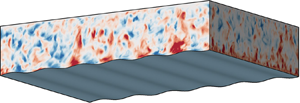
In this study we carry out wall-resolved large-eddy simulation (LES) of the turbulent wind field with the surface wave propagating in the opposite direction of the wind as sketched in figure 1. In the past two decades, because of their high fidelity, direct numerical simulation (DNS) and LES have played an increasingly important role in the study of turbulent wind–wave interaction (e.g. Sullivan, McWilliams & Moeng Reference Sullivan, McWilliams and Moeng2000; Sullivan et al. Reference Sullivan, Edson, Hristov and McWilliams2008; Yang & Shen Reference Yang and Shen2009, Reference Yang and Shen2010; Druzhinin, Troitskaya & Zilitinkevich Reference Druzhinin, Troitskaya and Zilitinkevich2012, Reference Druzhinin, Troitskaya and Zilitinkevich2016; Jiang et al. Reference Jiang, Sullivan, Wang, Doyle and Vincent2016; Yang & Shen Reference Yang and Shen2017; Akervik & Vartdal Reference Akervik and Vartdal2019; Hao & Shen Reference Hao and Shen2019; Wang et al. Reference Wang, Zhang, Hao, Huang, Shen, Xu and Zhang2020). The advantage of the wall-resolved LES is that it allows for a Reynolds number higher than the DNS, but still resolves the viscous sublayer near the wave surface, without the parameterizations of surface roughness and surface stress (Pope Reference Pope2000). From the wall-resolved LES, the three-dimensional turbulent wind field in the presence of the opposing water waves is obtained, and the wave-induced air motions are extracted and examined. To explain the arising of the wave-induced airflow, we also perform a theoretical analysis of the linearised viscous momentum equation for the wave-induced air motions in a mapped computational curvilinear coordinate in the presence of wind shear for the first time.

Figure 1. Sketch of the computational configuration of LES of a wind opposing water wave. The turbulent wind field is driven by a constant velocity  $U_0$ at the top of the computational domain, with the Dirichlet boundary condition applied at the wave surface and periodic boundary condition applied in the horizontal directions. The surface wave propagates in the
  $-x$ direction, with a wavelength
  $\lambda$, an amplitude
  $a$ and a phase speed
  $c$.
$c$.
The remainder of the paper is organized as follows. The configuration of simulation and the methodology for the statistical analysis are shown in § 2. The features of the wave-coherent airflow are illustrated in § 3. The derivation of the viscous linearised equation is provided in § 4, and the physical mechanisms underlying the wave-induced airflow are discussed in § 5. In § 6 we perform a comparison of the wave attenuation rate between the present study and the previous studies. At last, conclusions and discussion are given in § 7.
2. Configuration of simulation and methodology for data analysis
2.1. Configuration of simulation
To solve for the turbulent wind field following or opposing waves, we perform LES of wind turbulence over waves. The filtered Navier–Stokes (NS) equations for the air motions are given as
 \begin{gather} \frac{\partial u_j}{\partial x_j}=0, \end{gather}
 \begin{gather}\frac{\partial u_j}{\partial t}+u_m\frac{\partial u_j}{\partial x_m} =-\frac{1}{\rho_a}\frac{\partial p}{\partial x_j} -\frac{\partial\tau_{jm}^d}{\partial x_m}+\nu\frac{\partial^2u_j} {\partial x_m\partial x_m}, \end{gather}
where  $x$,
$x$,  $y$ and
  $z$ denote the coordinates (figure 1) in the streamwise, spanwise and vertical directions, respectively,
  $u_j (\,j=1,2,3)=(u,v,w)$ is the filtered velocity in LES at the grid scale,
  $p$ is the filtered modified pressure,
  $\tau _{jm}^d$ is the trace-free part of the subgrid-scale (SGS) stress tensor,
  $\rho _a$ is the density of air and
  $\nu$ is the kinematic viscosity of air.
The progressive waves are imposed as a Dirichlet boundary condition for the air velocity at the water surface,  $u_i(z=\eta )= (u_s, v_s, w_s)$, where
  $\eta$ is the surface wave elevation and
  $(u_s, v_s, w_s)$ is the orbital velocity of the wave at the surface, given as
 \begin{gather} \eta(x,y,z,t) = a\sin k(x-ct), \end{gather}
 \begin{gather}u_s(x,y,z,t) = akc\sin k(x-ct), \end{gather}
 \begin{gather}v_s(x,y,z,t) = 0, \end{gather}
 \begin{gather}w_s(x,y,z,t) = - akc\cos k(x-ct), \end{gather}
where  $a$ is the amplitude of the surface wave,
  $k=2{\rm \pi} /\lambda$ is the wavenumber,
  $\lambda$ is the wavelength and
  $c$ is the phase speed. Here, an Airy wave solution is adopted. In the case of a Stokes wave, the effect of nonlinearity by the higher harmonics is of
  $O((ak)^2)$. In our derivation and analysis of the linearised equations in the following sections, the
  $O((ak)^2)$ terms in the governing equations are neglected. Therefore, we only consider the dominant Fourier component in the water wave solution to be consistent.
To accurately capture the effects of the surface wave geometry and motions on the turbulent wind field, the LES solver utilizes a boundary-fitted grid that follows the instantaneous wave surface at each time step. For discretizing the governing equations, we transform the irregular physical domain  $(x, y, z, t)$ above the wave to a rectangular computational domain
  $(\xi , \psi , \zeta , \tau )$ using the following algebraic mapping:
 \begin{equation} \tau=t,\quad \xi=x,\quad \psi=y,\quad \zeta=z+g(\zeta)\eta, \quad \mbox{where}\ g(\zeta) = \frac{\zeta}{H}-1. \end{equation}
Here,  $H$ is the mean physical domain height and
  $g(\zeta )$ denotes the transformation function. We use the index notation to denote the physical and computational coordinates as
  $x_j(\,j=1, 2, 3)=(x,y,z)$ and
  $\xi _j(\,j=1, 2, 3)=(\xi ,\psi ,\zeta )$, respectively. The Jacobian matrix corresponding to the above transformation is
 \begin{equation} \boldsymbol{J}=\left[ \begin{array}{@{}ccc@{}} \displaystyle \dfrac{\partial{\xi}}{\partial x} & \displaystyle \dfrac{\partial{\xi}}{\partial y} & \displaystyle \dfrac{\partial{\xi}}{\partial z} \\ \displaystyle \dfrac{\partial{\psi}}{\partial x} & \displaystyle \dfrac{\partial{\psi}}{\partial y} & \displaystyle \dfrac{\partial{\psi}}{\partial z} \\ \displaystyle \dfrac{\partial{\zeta}}{\partial x} & \displaystyle \dfrac{\partial{\zeta}}{\partial y} & \displaystyle \dfrac{\partial{\zeta}}{\partial z} \end{array} \right] =\left[ \begin{array}{cccc} 1 & 0 & 0 \\ 0 & 1 & 0 \\ \displaystyle \dfrac{g\eta_\xi} {1-g_\zeta \eta} & \displaystyle \dfrac{g\eta_\psi} {1-g_\zeta \eta} & \displaystyle \dfrac{1} {1-g_\zeta \eta} \end{array} \right], \end{equation}
where  $g_\zeta = \mathrm {d} g / \mathrm {d} \zeta$. Because of the surface wave motions, the transformation (2.7) varies with time, resulting in a transformation of time derivative between the computational space and the physical space
 \begin{equation} \frac{\partial}{\partial t} = \frac{\partial}{\partial \tau} + \frac{\partial{\xi_j}}{\partial t} \frac{\partial}{\partial \xi_j} = \frac{\partial}{\partial \tau} + \frac{\partial{\zeta}}{\partial t} \frac{\partial}{\partial \zeta}, \quad \mbox{where} \ \frac{\partial{\zeta}}{\partial t} = \frac{g\eta_\tau} {1-g_\zeta \eta}. \end{equation}
The transformed LES equations in the computational space read as
 \begin{gather} J_{pj} \frac{\partial u_j}{\partial \xi_p} = 0, \end{gather}
 \begin{gather}\frac{\partial u_j}{\partial \tau} + \delta_{p3} \frac{\partial{\zeta}}{\partial t} \frac{\partial u_j}{\partial \xi_p} + J_{lp} \frac{\partial (u_j u_p)}{\partial \xi_l} = - \frac{J_{lj} }{\rho_a} \frac{\partial p}{\partial \xi_l} + J_{lp} \frac{\partial \tau_{jp}^d}{\partial \xi_l} + \nu J_{np} \frac{\partial}{\partial{\xi_n}} \left( J_{lp} \frac{\partial u_j}{\partial{\xi_l}} \right), \end{gather}
where  $J_{lp}$ is the
  $(l,p)$ entry of the mapping matrix
  $\boldsymbol {J}$ and
  $\delta _{lp}$ is the Kronecker delta.
Equations (2.10) and (2.11) are discretized and solved in the rectangular computational space. A Fourier-series-based pseudo-spectral method is used for the  $(\xi , \psi )$ plane discretization with evenly spaced grid points in both directions. A second-order finite difference method is employed for the discretization in the
  $\zeta$ direction with grid points clustered near the upper and lower boundaries. For the filtering operators in the LES, a two-dimensional spectral cutoff filter in the
  $(\xi , \psi )$ plane is adopted. In the momentum equation the SGS stress tensor is calculated using the dynamic Smagorinsky model (Smagorinsky Reference Smagorinsky1963; Germano et al. Reference Germano, Piomelli, Moin and Cabot1991; Lilly Reference Lilly1992). To integrate the momentum equations in time, we use a fractional-step method. First, the advection and viscous terms are advanced in time with the second-order Adam–Bashforth scheme. Second, a nonlinear Poisson equation is solved using iteration to obtain the pressure field, which is used to correct the velocity field such that the continuity equation is satisfied. The detailed numerical procedure and the validation of our numerical method can be found in Yang & Shen (Reference Yang and Shen2011a). The present LES solver simulates the system in a time-dependent domain. The solver was developed for turbulent airflows over a complex wave field (Yang & Shen Reference Yang and Shen2011a,Reference Yang and Shenb). The conservation of momentum is examined in appendix A. The present solver has been extensively utilized to study a turbulent wind field in the presence of monochromatic water waves (Yang & Shen Reference Yang and Shen2009, Reference Yang and Shen2010, Reference Yang and Shen2017) and broadband water wave fields (Yang, Meneveau & Shen Reference Yang, Meneveau and Shen2013, Reference Yang, Meneveau and Shen2014a,Reference Yang, Meneveau and Shenb; Hao & Shen Reference Hao and Shen2019), with extensive validations performed in the references cited above. We note that for monochromatic waves, it is also feasible to perform the simulation in the frame travelling with the wave, where the domain geometry does not change in time (e.g. Sullivan et al. Reference Sullivan, McWilliams and Moeng2000; Druzhinin et al. Reference Druzhinin, Troitskaya and Zilitinkevich2012).
As sketched in figure 1, the turbulent wind is driven by a fixed velocity at the top of the simulation domain:  $(u, v, w)=(U_0, 0, 0)$, and a periodic boundary condition is applied in the horizontal directions on the lateral boundaries. This canonical setup has been extensively used in the previous simulations of turbulent air flows over surface waves (e.g. Sullivan et al. Reference Sullivan, McWilliams and Moeng2000; Druzhinin et al. Reference Druzhinin, Troitskaya and Zilitinkevich2012, Reference Druzhinin, Troitskaya and Zilitinkevich2016). In the present study the wave age
  $c/U_0$ of the waves varies between
  $-0.8$ and
  $0.1$. Two wave steepness values are considered,
  $ak=0.08$ and
  $0.15$ (table 1). Here, a negative wave age denotes the surface wave propagating against the wind direction, while a positive wave age denotes the following-wind surface wave. The wave steepness in the present study is comparable to the typical values adopted in the previous studies of wind opposing waves, e.g.
  $ak = 0.06-0.19$ in Peirson et al. (Reference Peirson, Garcia and Pells2003) and
  $ak \approx 0.06\text {--}0.13$ in Mitsuyasu & Yoshida (Reference Mitsuyasu and Yoshida2005). The Reynolds number based on the wavelength of the surface wave and the driving velocity at the top,
  $U_0\lambda /\nu$, is 30 000, which is higher than the previous DNS of wind over water waves, e.g. 8800 in Sullivan et al. (Reference Sullivan, McWilliams and Moeng2000), 10 000 in Yang & Shen (Reference Yang and Shen2010) and 15 000 in Druzhinin et al. (Reference Druzhinin, Troitskaya and Zilitinkevich2012), but is one to two orders of magnitude lower than the laboratory studies of wind opposing waves (Young & Sobey Reference Young and Sobey1985; Peirson et al. Reference Peirson, Garcia and Pells2003; Mitsuyasu & Yoshida Reference Mitsuyasu and Yoshida2005) as limited by the computation cost of the wall-resolved LES. However, as reviewed by Sullivan & McWilliams (Reference Sullivan and McWilliams2010), despite the lower Reynolds number, DNS and LES are capable of revealing many key physical processes in the turbulent wind–wave interaction. The corresponding Reynolds number based on the friction velocity
  $u_\tau \lambda /\nu$ varies slightly from case to case, but is around
  $800$ for all cases as summarized in table 1. Here,
  $u_\tau$ is defined as the friction velocity
  $u_\tau =\sqrt {\tau _s/\rho _a}$, where
  $\tau _s$ is the mean viscous shear stress at the top of the simulation domain, which equals the mean total stress at any given height in the wave surface layer and the summation of viscous shear stress and form drag at the wave surface.
Table 1. List of LES cases for turbulent wind opposing and following progressive water waves. In the table WFW stands for wind following wave and WOW for wind opposing wave. The bulk Reynolds number  $U_0\lambda /\nu$ is prescribed as 30 000 for all the wave cases, while
  $u_\tau \lambda /\nu$ and the grid resolution are quantified a posterior.

To fully capture the wave-coherent motions in the wind field, a simulation domain of the size  $(L_x, L_y, H) = (6\lambda , 4\lambda , \lambda )$ is adopted. The same domain size has been employed in the previous studies (e.g. Sullivan et al. Reference Sullivan, McWilliams and Moeng2000; Druzhinin et al. Reference Druzhinin, Troitskaya and Zilitinkevich2012, Reference Druzhinin, Troitskaya and Zilitinkevich2016). The turbulent flow field is discretized in the computational space with
  $384^2\times 192$ grid points, providing a resolution of
  ${\rm \Delta} \xi ^+ \simeq 21$,
  ${\rm \Delta} \psi ^+ \simeq 14$, and
  ${\rm \Delta} \zeta _{{min}}^+ \simeq 0.2$, where
  ${\rm \Delta} \zeta _{{min}}^+$ denotes the minimum grid space near the boundary in the
  $\zeta$ direction. The superscript ‘
 $+$’ indicates normalisation by the viscous length scale
  $\nu / u_\tau$. The grid resolution is sufficient for wall-resolved LES according to the criterion given in Choi & Moin (Reference Choi and Moin2012), and we have confirmed the grid convergence with tests described in appendix B. The parameters and resolution of the wave cases considered in this study are summarized in table 1.
For data sampling, the simulations of all cases evolve for approximately  $120$ times of the largest eddy turnover time, i.e.
  $120 H/u_\tau$. Snapshots of three dimensional instantaneous velocity fields were output every
  $0.17 H/u_\tau$, corresponding to
  $150$ viscous time units, i.e.
  $150\nu /u_\tau ^2$, with a total number of 200 snapshots for the statistical analysis in this study.
2.2. Methodology for data analysis
To extract the effects of the progressive water waves on the overlying turbulent wind field, we apply a triple decomposition to the instantaneous flow field (Hussain & Reynolds Reference Hussain and Reynolds1970)
 \begin{equation} f(x,y,z,t)=\bar{f}(\xi, \zeta) + f'(x, y, z, t) = \langle\,f \rangle(\zeta) + \tilde{f}(\xi, \zeta) + f'(x, y, z, t), \end{equation}
where  $f$ denotes an arbitrary physical quantity in the wind field,
  $\bar {f}$ is its phase-averaged part,
  $\langle\,f \rangle$ is its mean value, which is obtained through the average in time and over the
  $(\xi , \psi )$ plane,
  $\tilde {f}$ is its wave-induced fluctuation and
  $f'$ is its turbulent fluctuation. The phase-averaged quantify
  $\bar {f}$ is calculated using the snapshots of the turbulent flow field with two steps: first, because the wave phase is known at each time step from the prescribed surface elevation information (2.3) with
  $k(\xi -ct)$ quantified, each instantaneous flow field is averaged along the spanwise direction and then shifted to the same phase with respect to the surface wave; then an ensemble average of the shifted velocity fields is performed
 \begin{equation} \bar{f}(\xi, \zeta) = \frac{1}{N_t} \frac{1}{N_y} \sum_{p=1}^{N_t} \sum_{m=1}^{N_y} f(\xi(l)-ct(p), \psi(m), \zeta(n)), \end{equation}
where the indices  $l$,
$l$,  $m$,
$m$,  $n$,
$n$,  $p$ denote the discrete points in
  $\xi$,
  $\psi$,
  $\zeta$, and
  $t$, respectively, and
  $N_t$ and
  $N_y$ are the total number of the snapshots employed and the number of the grid points in the spanwise direction, respectively. Then the turbulent fluctuation is calculated by subtracting the phase-averaged part from the instantaneous part, i.e.
  $f'(x, y, z, t)=f(x, y, z, t)-\bar {f}(\xi , \zeta )$, and the wave-induced part is obtained by subtracting the mean value from the phase-averaged quantity, i.e.
  $\tilde {f}(\xi , \zeta ) = \bar {f}(\xi , \zeta ) - \langle\,f \rangle (\zeta )$.
In (2.12),  $\tilde {f}$ is the Cartesian wave-coherent quantity, with the physical coordinate
  $(x,y,z)$ transformed to the mapped curvilinear coordinate
  $(\xi ,\psi ,\zeta )$. Although performing average in the
  $(x,y,z)$ coordinate has the advantage of being independent of the mapped computational curvilinear grid,
  $\tilde {f}$ is not defined for all of the region below the wave crest and above the wave trough. Moreover, for theoretical analysis, because the boundary conditions imposed by the wave elevation and kinematics for the airflow are applied on a curved surface, it is challenging to derive the boundary conditions for
  $\tilde {f}$ in the
  $(x,y,z)$ coordinate. Therefore, many previous experimental, numerical and theoretical studies conducted averaging in the mapped curvilinear coordinates (e.g. Hsu et al. Reference Hsu, Hsu and Street1981; Hsu & Hsu Reference Hsu and Hsu1983; Belcher & Hunt Reference Belcher and Hunt1993; Sullivan et al. Reference Sullivan, McWilliams and Moeng2000; Yang & Shen Reference Yang and Shen2010; Hara & Sullivan Reference Hara and Sullivan2015; Buckley & Veron Reference Buckley and Veron2016; Akervik & Vartdal Reference Akervik and Vartdal2019). Using the various forms of mapped coordinates employed in previous studies, the underlying physical mechanisms revealed are the same (see, e.g. Yang & Shen Reference Yang and Shen2010; Hara & Sullivan Reference Hara and Sullivan2015).
Previous studies showed that  $\tilde {f}$ is dominated by its fundamental mode, i.e. the Fourier coefficient
  $\hat {f}$ corresponding to the wavenumber
  $k$ (Hussain & Reynolds Reference Hussain and Reynolds1970),
 \begin{equation} \tilde{f}=\hat{f}\,\mathrm{e}^{\mathrm{i}k\xi} + \hat{f}^*\mathrm{e}^{-\mathrm{i}k\xi} + \text{harmonics}, \end{equation}
where  $\hat {f}^*$ is the complex conjugate of
  $\hat {f}$. The phase difference between
  $\tilde {f}$ and
  $\tilde {\eta }$ is quantified according to
 \begin{equation} \tilde{f}=2\,\textrm{Re} [\hat{f}]\cos(k\xi)-2\,\textrm{Im}[\hat{f}]\sin(k\xi) = 2| \hat{f}|\sin(k\xi-\phi_{\tilde{f}\tilde{\eta}})+ \text{harmonics}. \end{equation}
Here, ‘ $|\cdot |$’ is the modulus operator for complex numbers and
  $\phi _{\tilde {f}\tilde {\eta }}=\arctan (\textrm {Re}[\hat {f}]/\textrm {Im}[\hat {f}])$ is the phase difference from the wave surface
  $\tilde {\eta } =a\sin (k\xi )$. For the analyses in §§ 4 and 5, we focus on the fundamental mode of the wave-induced quantity, following the previous studies (e.g. Miles Reference Miles1957; Hsu et al. Reference Hsu, Hsu and Street1981; Hsu & Hsu Reference Hsu and Hsu1983; Belcher & Hunt Reference Belcher and Hunt1993; Kihara et al. Reference Kihara, Hanazaki, Mizuya and Ueda2007). The real and imaginary parts of
  $\hat {f}$ have different spatial structures and different physical meanings. Specifically,
  $\textrm {Re}[\hat {f}]$ corresponds to a cosinusoidal perturbation, which is
  ${\rm \pi} /2$ out-of-phase with the wave surface, while
  $\textrm {Im}[\hat {f}]$ corresponds to a sinusoidal perturbation, which is in-phase with the wave surface. In other words,
  $\textrm {Re}[\hat {f}]$ is antisymmetric about the surface wave crest, while
  $\textrm {Im}[\hat {f}]$ has a symmetric spatial distribution.
It is noted that the phase average is adopted to extract the wave-induced quantity  $\tilde {f}$ in the triple decomposition (2.12), which has been widely employed in studies where the effects of a monochromatic wave or the dominant wave component of the wind waves are considered (e.g. Hsu et al. Reference Hsu, Hsu and Street1981; Hsu & Hsu Reference Hsu and Hsu1983; Sullivan et al. Reference Sullivan, McWilliams and Moeng2000; Kihara et al. Reference Kihara, Hanazaki, Mizuya and Ueda2007; Yang & Shen Reference Yang and Shen2010; Druzhinin et al. Reference Druzhinin, Troitskaya and Zilitinkevich2012; Hara & Sullivan Reference Hara and Sullivan2015; Buckley & Veron Reference Buckley and Veron2016; Yang & Shen Reference Yang and Shen2017; Akervik & Vartdal Reference Akervik and Vartdal2019). The wave-coherent quantity can also be identified through the correlation with the wave elevation (Hristov, Friehe & Miller Reference Hristov, Friehe and Miller1998; Hristov & Ruiz-Plancarte Reference Hristov and Ruiz-Plancarte2014) or through the spectral method (Grare, Lenain & Melville Reference Grare, Lenain and Melville2013a, Reference Grare, Lenain and Melville2018). For the monochromatic wave form considered in the present study, the difference among these methods is small as the wave-induced quantity is dominated by the fundamental mode. However, the latter two methods have the advantage of being able to extract the wave-coherent quantity above a broadband wave field.
In the following sections we first show the opposing wave effects on the velocity, pressure and turbulence statistics in the airflow (§ 3). In § 4 we present a physical model to explain the opposing wave-induced airflow. The underlying physical mechanisms and the wave attenuation rate are examined in §§ 5 and 6, respectively. We note that in §§ 3 and 5, we focus on four representative wave cases in table 1, namely WFW01 ( $c/U_0=0.1$,
  $ak=0.15$), WOW01 (
 $c/U_0=-0.1$,
  $ak=0.15$), WOW01L (
 $c/U_0=-0.1$,
  $ak=0.08$) and WOW04 (
 $c/U_0=-0.4$,
  $ak=0.15$), to show the effects of wave propagation direction, wave steepness and wave speed. The other wave cases have consistent results as the four wave cases and thus are not presented in these two sections for space and clarity consideration. In § 6 we present the wave attenuation rates in all of the wave cases listed in table 1 to compare with previous studies.
3. Features of opposing wave effects in the airflow
In this section we show the wave-coherent velocity (§ 3.1), wave-coherent stress  $-\tilde {u}\tilde {w}$ and pressure
  $\tilde {p}$ (§ 3.2), and wave-coherent turbulence variance
  $\widetilde {u'u'}+\widetilde {w'w'}$ and turbulent stress
  $-\widetilde {u'w'}$ (§ 3.3) in the wall-resolved LES. Note that in the expressions of the wave-coherent stress and turbulent stress used here, the constant air density is omitted.
3.1. Wave-induced velocity
The propagation of a surface wave can induce velocity perturbation in the airflow travelling at the same speed as the surface wave celerity, which is usually referred to as the ‘wave-coherent’ or ‘wave-induced’ velocity in the literature. For a plane progressive gravity wave, the wave-induced velocity also exhibits a two-dimensional pattern. In the instantaneous fields the perturbations by the wave are more pronounced in the vertical velocity than in the streamwise velocity owing to the mean shear in the latter. Therefore, we use the instantaneous vertical velocity to illustrate the effects of water waves. Figure 2 shows snapshots of the vertical velocity for the four wave conditions: WFW01, WOW01, WOW01L and WOW04 (table 1). For the same wave speed, both the following wave case WFW01 (figure 2a) and the opposing wave case WOW01 (figure 2b) display a structure of alternating positive and negative vertical velocity  $w$, which corresponds to upward and downward airflow along the wave crest, respectively, with the magnitude in the opposing wave case being slightly larger especially near the wave surface. The strength of this flow structure varies with wave steepness and speed. Compared with case WOW01 (figure 2b), the velocity perturbation becomes weaker for a less steep opposing wave in case WOW01L (figure 2c), while it is strengthened for a faster opposing wave in case WOW04 (figure 2d).

Figure 2. Instantaneous field of the vertical velocity  $w$, normalised by the top-driven velocity
  $U_0$, for the simulation cases: (a) WFW01,
  $c/U_0=0.1$,
  $ak=0.15$; (b) WOW01,
  $c/U_0=-0.1$,
  $ak=0.15$; (c) WOW01L,
  $c/U_0=-0.1$,
  $ak=0.08$; (d) WOW04,
  $c/U_0=-0.4$,
  $ak=0.15$. For positive wave age, the surface wave travels in the
  $+x$ direction, while for negative wave age, the surface wave travels in the
  $-x$ direction. The wind is along with the
  $+x$ direction in all cases.
To show the statistical results of the structure of the upward and downward wave-coherent airflows, we present the wave-induced vertical velocity  $\tilde {w}$ in figure 3. It is noted that in figure 3, the contours are plotted up to
  $z/\lambda =0.4$, because the magnitudes of wave-induced quantities are small above this height, which is also the case for the other figures in §§ 3 and 5. In general, the opposing wave cases (figure 3b–d) show a positive
  $\tilde {w}$ at the windward face and a negative
  $\tilde {w}$ at the leeward side with a nearly antisymmetric structure throughout the wave boundary layer, indicating that its phase difference from the wave profile
  $\tilde {\eta }$ is roughly
  ${\rm \pi} /2$. In the following wave case (figure 3a), although
  $\tilde {w}$ is positive at the windward face and negative at the leeward face as in the opposing wave cases, it does not display antisymmetry. Near the wave surface,
  $\tilde {w}$ is tilted because of the effect of wave orbital velocity at the surface, which induces a negative
  $\tilde {w}$ at the windward side below the critical height (which is comparable to the viscous sublayer thickness in case WFW01 which has
  $c/u_\tau < 5$). Hence, the region corresponding to negative
  $\tilde {w}$ transits sharply from the windward face to the leeward face across the critical height, resulting in the tilting of
  $\tilde {w}$ near the wave surface. As the Reynolds number increases, the viscous sublayer becomes thinner compared to the wavelength and correspondingly the transition of
  $\tilde {w}$ occurs in a thinner region in the airflow, which causes the tilting of
  $\tilde {w}$ to be less obvious as shown in the case
  $(c/u_\tau , ak) = (3.7, 0.13)$ in Buckley & Veron (Reference Buckley and Veron2016). This phenomenon does not happen in the opposing wave cases, as the pattern of
  $\tilde {w}$ induced by the wave kinematics at the wave surface is the same as the behaviour of
  $\tilde {w}$ away from the wave surface. Also shown in figure 3 is that not only the spatial structure but also the magnitude of
  $\tilde {w}$ is affected by the wave conditions. A comparison of the magnitude of
  $\tilde {w}$ between cases WFW01 (figure 3a) and WOW01 (figure 3b) shows that the wave propagating against the wind induces stronger
  $\tilde {w}$ than that induced by the wave following the wind. Additionally, compared with case WOW01, a less steep opposing wave causes a weaker
  $\tilde {w}$ (figure 3c), while a faster opposing wave results in a larger magnitude of
  $\tilde {w}$ (figure 3d), which is consistent with the observation in figure 2.

Figure 3. Spatial distribution of the wave-induced vertical velocity  $\tilde {w}$ for the wave conditions: (a) WFW01,
  $c/U_0=0.1$,
  $ak=0.15$; (b) WOW01,
  $c/U_0=-0.1$,
  $ak=0.15$; (c) WOW01L,
  $c/U_0=-0.1$,
  $ak=0.08$; (d) WOW04,
  $c/U_0=-0.4$,
  $ak=0.15$. The results are normalised by
  $u_\tau$.
Figure 4 shows the spatial distribution of the wave-induced streamwise velocity  $\tilde {u}$ for the wave conditions corresponding to figure 3. For the opposing waves, on the contrary to the antisymmetric distribution of
  $\tilde {w}$,
  $\tilde {u}$ displays nearly symmetric spatial distribution about the wave crest away from the wave surface (figure 4b–d), which is not exhibited in the following wave case (figure 4a). However, near the opposing wave surface,
  $\tilde {u}$ deviates from the symmetric distribution noticeably and reaches its maximum on the windward side near the wave crest, which is similar to the following wave case. While the spatial structure of
  $\tilde {u}$ is similar among different opposing wave cases, its magnitude varies with the opposing wave parameters. Similar to
  $\tilde {w}$, the magnitude of
  $\tilde {u}$ increases with the wave speed and wave steepness.

Figure 4. Spatial distribution of the wave-induced streamwise velocity  $\tilde {u}$ for the wave conditions: (a) WFW01,
  $c/U_0=0.1$,
  $ak=0.15$; (b) WOW01,
  $c/U_0=-0.1$,
  $ak=0.15$; (c) WOW01L,
  $c/U_0=-0.1$,
  $ak=0.08$; (d) WOW04,
  $c/U_0=-0.4$,
  $ak=0.15$. The results are normalised by
  $u_\tau$.
We note that although a strong negative  $\tilde {u}$ is present near the surface at the leeward face in all of the four wave cases, no apparent flow separation is observed in the mean flow. While the flow separation past a steady sinusoidal wavy surface was found to cause a recirculation zone downstream of the wave crest (e.g. Buckles, Hanratty & Adrian Reference Buckles, Hanratty and Adrian1984), the feature and criterion for the occurrence of airflow separation over water waves are still not fully understood, especially when the waves do not break, as pointed out by Buckley & Veron (Reference Buckley and Veron2016). For the non-breaking following waves, airflow separation has been found to happen only sporadically in the instantaneous field, and is difficult to visualize in the mean field. For instance, in their experimental studies, Veron, Saxena & Misra (Reference Veron, Saxena and Misra2007) and Buckley & Veron (Reference Buckley and Veron2016) only visualized the airflow separation in individual detachment events. In DNS, Yang & Shen (Reference Yang and Shen2010) and Druzhinin et al. (Reference Druzhinin, Troitskaya and Zilitinkevich2012) found that although airflow separation presents occasionally in the instantaneous flow field, no apparent separation in the mean flow is observed. For opposing waves, the study of airflow separation has received even less attention in the research literature and requires data of turbulent wind opposing waves with the wave steepness and Reynolds numbers systematically varied, which should be considered in future studies with a large number of simulation cases conducted.
As a summary of this subsection, the LES results illustrate the key features of the wave-induced vertical velocity  $\tilde {w}$ and streamwise velocity
  $\tilde {u}$ under the opposing wave condition. The
  $\tilde {w}$ appears antisymmetric throughout the wave boundary layer while
  $\tilde {u}$ is symmetric away from the surface, which has led some previous studies to use potential flow theory to explain their arising. However, near the wave surface,
  $\tilde {u}$ is no longer symmetric, suggesting that the potential flow theory is inadequate to describe the flow dynamics. The detailed physical mechanisms for
  $\tilde {w}$ and
  $\tilde {u}$ are investigated in §§ 5.1 and 5.2, respectively.
3.2. Wave-induced stress and pressure
The proceeding subsection shows that the wave direction is a key factor in determining the pattern of wave-induced velocity. Consequently, the wave-coherent stress,  $-\tilde {u}\tilde {w}$, also reflects the impact of the wave direction, which is shown in figure 5. In the following wave case WFW01 (which has
  $c/u_\tau =3.46$),
  $-\tilde {u}\tilde {w}$ is mostly negative, especially near the wave surface (figure 5a), which is consistent with the results of the case
  $(c/u_\tau , ak) = (3.7, 0.13)$ in Buckley & Veron (Reference Buckley and Veron2016), but is different from the pattern in the case
  $(c/u_\tau , ak) = (6.27, 0.07)$ in Yousefi et al. (Reference Yousefi, Veron and Buckley2020) because the latter used curvilinear coordinate variables to define the wave-coherent stress. The corresponding opposing wave (figure 5b) results in alternating positive and negative
  $-\tilde {u}\tilde {w}$ along the wave surface, which displays an antisymmetric distribution away from the surface. This feature of
  $-\tilde {u}\tilde {w}$ is also exhibited by the other two opposing wave cases (figures 5c and 5d), and is caused by the nearly antisymmetric
  $\tilde {w}$ and symmetric
  $\tilde {u}$ (figures 3 and 4). Near the wave surface, because
  $\tilde {u}$ deviates from the symmetric distribution,
  $-\tilde {u}\tilde {w}$ no longer exhibits antisymmetry there.

Figure 5. Spatial distribution of the wave-induced stress  $-\tilde {u}\tilde {w}$ for the wave conditions: (a) WFW01,
  $c/U_0=0.1$,
  $ak=0.15$; (b) WOW01,
  $c/U_0=-0.1$,
  $ak=0.15$; (c) WOW01L,
  $c/U_0=-0.1$,
  $ak=0.08$; (d) WOW04,
  $c/U_0=-0.4$,
  $ak=0.15$. The results are normalised by
  $u_\tau ^2$.
In addition to  $-\tilde {u}\tilde {w}$, surface waves also induce pressure perturbation in the airflow to impact the momentum flux. Previous laboratory and field measurements have reported that the pressure induced by opposing waves is nearly symmetric about the surface wave crest (Snyder et al. Reference Snyder, Dobson, Elliott and Long1981; Young & Sobey Reference Young and Sobey1985; Hasselmann & Bösenberg Reference Hasselmann and Bösenberg1991), which is also reflected in the present LES results. In figure 6 we plot the spatial distribution of
  $\tilde {p}$ for the four wave conditions. It is obvious that for the same wave parameters, the pressure induced by the opposing wave (figure 6b) is much stronger and more symmetric about the wave crest compared with that induced by the following wave (figure 6a). In the latter case, the pressure distribution is mostly positive on the windward face of the wave and negative on the leeward side. The seemingly symmetric distribution of
  $\tilde {p}$ induced by opposing waves is also present with a lower wave steepness (figure 6c) and a faster wave speed (figure 6d).

Figure 6. Spatial distribution of the wave-induced pressure  $\tilde {p}$ for the wave conditions: (a) WFW01,
  $c/U_0=0.1$,
  $ak=0.15$; (b) WOW01,
  $c/U_0=-0.1$,
  $ak=0.15$; (c) WOW01L,
  $c/U_0=-0.1$,
  $ak=0.08$; (d) WOW04,
  $c/U_0=-0.4$,
  $ak=0.15$. The results are normalised by
  $\rho _a u_\tau ^2$.
In this subsection the LES results show that the opposing waves induce nearly antisymmetric wave-coherent stress  $-\tilde {u}\tilde {w}$ away from the wave surface, and nearly symmetric wave-coherent pressure
  $\tilde {p}$ throughout the wave boundary layer. Similar to
  $\tilde {w}$ and
  $\tilde {u}$, the pattern of
  $-\tilde {u}\tilde {w}$ and
  $\tilde {p}$ are similar among the different opposing wave cases, but with their magnitudes varying. The detailed physical mechanisms for
  $-\tilde {u}\tilde {w}$ and
  $\tilde {p}$ are investigated in § 5.3.
3.3. Wave-induced turbulence variance and turbulent stress
In this subsection we examine the modulation of turbulence variance  $u'u'+w'w'$ and turbulent stress
  $-u'w'$ by the opposing waves. In the present study, the turbulence variance and turbulent stress are defined using the variables in the Cartesian coordinate. Adopting definitions based on the curvilinear coordinate variables may result in a different appearance, as discussed in Yousefi et al. (Reference Yousefi, Veron and Buckley2020). Figure 7 presents the spatial distribution of the wave-induced turbulence variance
  $\widetilde {u'u'}+\widetilde {w'w'}= \bar {u'u'} - \langle u'u' \rangle +\bar {w'w'} - \langle w'w' \rangle$ (see § 2.2 for definitions of averaging) for different wave conditions to illustrate how the turbulence intensity is affected by the presence of surface waves. It is shown that in the following wave case WFW01 (figure 7a) there is a strong positive
  $\widetilde {u'u'}+\widetilde {w'w'}$ above the leeward face of the wave. In the corresponding opposing wave case WOW01 (figure 7b), the region for the intensified turbulence variance moves further downstream towards the wave trough. More importantly, in the opposing wave case WOW01, the region for strong
  $\widetilde {u'u'}+\widetilde {w'w'}$ is concentrated in a much thinner region compared with the following wave case WFW01. In the less steep wave case WOW01L (figure 7c), the pattern of
  $\widetilde {u'u'}+\widetilde {w'w'}$ is similar to case WOW01 but with a smaller magnitude. In the fast opposing wave case WOW04 (figure 7d),
  $\widetilde {u'u'}+\widetilde {w'w'}$ is much weaker and is confined within an even thinner region compared with case WOW01.

Figure 7. Spatial distribution of the wave-induced turbulence variance  $\widetilde {u'u'}+\widetilde {w'w'}$ for the wave conditions: (a) WFW01,
  $c/U_0=0.1$,
  $ak=0.15$; (b) WOW01,
  $c/U_0=-0.1$,
  $ak=0.15$; (c) WOW01L,
  $c/U_0=-0.1$,
  $ak=0.08$; (d) WOW04,
  $c/U_0=-0.4$,
  $ak=0.15$. The results are normalised by
  $u_\tau ^2$.
In figure 8 we plot the spatial distribution of the wave-induced turbulent shear stress  $-\widetilde {u'w'}= -\bar {u'w'} - \langle -u'w' \rangle$ for different wave conditions, which quantifies how the turbulent shear stress
  $-u'w'$ is modulated by the presence of surface waves. The comparison between cases WFW01 (figure 8a) and WOW01 (figure 8b) shows that, near the wave surface, both the following wave and opposing wave induce a negative
  $-\widetilde {u'w'}$ at the windward side and a positive
  $-\widetilde {u'w'}$ further downstream. However, the strong
  $-\widetilde {u'w'}$ is limited to a much thinner region in the opposing wave cases, which is similar to the behaviour of
  $\widetilde {u'u'}+\widetilde {w'w'}$ shown in figure 7. Furthermore, the region of strong
  $-\widetilde {u'w'}$ becomes even thinner as the opposing wave becomes faster in case WOW04 (figure 8d). Away from the wave surface,
  $-\widetilde {u'w'}$ is relatively weak and exhibits a quasi-antisymmetric spatial distribution about the wave crest for the opposing wave cases WOW01 and WOW04, which is not observed in the following wave case WFW01 for the same wave steepness.

Figure 8. Spatial distribution of the wave-induced turbulent stress  $-\widetilde {u'w'}$ for the wave conditions: (a) WFW01,
  $c/U_0=0.1$,
  $ak=0.15$; (b) WOW01,
  $c/U_0=-0.1$,
  $ak=0.15$; (c) WOW01L,
  $c/U_0=-0.1$,
  $ak=0.08$; (d) WOW04,
  $c/U_0=-0.4$,
  $ak=0.15$. The results are normalised by
  $u_\tau ^2$.
To summarize this subsection, we have observed that the strong opposing wave-induced turbulence variance and turbulent stress is limited to a much thinner region in the airflow, compared with the wind over a slow following wave case. This result is consistent with the conclusion we obtain in § 5.1.2 below that the region where the in-phase component of  $\tilde {w}$ is affected by the wave-induced turbulent stress is much thinner for the opposing wave than the corresponding following wave.
To conclude § 3, we have investigated the features of wave-induced velocity, pressure and turbulence statistics in the opposing wave condition. Next, we present a viscous linearised model for  $\tilde {w}$ in the mapped computational curvilinear coordinate in § 4, based on which the physical mechanisms underlying the arising of the opposing wave-induced airflow
  $\tilde {w}$,
  $\tilde {u}$,
  $-\tilde {u}\tilde {w}$ and
  $\tilde {p}$ shown in § 3 are explained in § 5.
4. Viscous linearised model for the opposing wave effects
In § 3 we have shown the key characteristics of the opposing wave effects on the velocity, pressure and turbulence statistics in the airflow based on the LES data. To investigate the mechanisms underlying the opposing wave effects, in this section, we develop a new viscous model for the wave-induced velocity by linearising the phase-averaged Navier–Stokes equations for the mean wind velocity in the mapped computational curvilinear coordinate.
The transformation between the physical coordinate  $(x,y,z)$ and mapped computational curvilinear coordinate
  $(\xi , \psi , \zeta )$ given by (2.7) is non-orthogonal and follows the form of Hsu et al. (Reference Hsu, Hsu and Street1981) and Hsu & Hsu (Reference Hsu and Hsu1983), which has been widely adopted in the literature to study the wave-induced quantities using a variety of mapping functions (e.g. Snyder et al. Reference Snyder, Dobson, Elliott and Long1981; Young & Sobey Reference Young and Sobey1985; Mastenbroek Reference Mastenbroek1996; Yang & Shen Reference Yang and Shen2010; Hara & Sullivan Reference Hara and Sullivan2015; Akervik & Vartdal Reference Akervik and Vartdal2019). As suggested by Hsu et al. (Reference Hsu, Hsu and Street1981), in principle, any function
  $g$ can be considered if it satisfies
  $g(0)=-1$ and increases monotonically to zero at the top of the boundary layer. A function that satisfies this condition guarantees that the transformation is one to one but may result in sampling points that are not at the ideal offset, e.g. constant distance, from the wave surface, and the resulting transformed coordinate is not necessarily aligned with the mean streamlines. The use of the transformation of the form (2.7) has been able to reveal important results of the turbulent wind–wave interaction (see the above mentioned studies). In the following derivation we assume that the transformation follows the form of (2.7), but we do not specify a particular transformation function
  $g$.
$g$.
To derive the viscous linearised model, we use the LES equations in the mapped computational curvilinear coordinate in the strongly conservative form (e.g. Hara & Sullivan Reference Hara and Sullivan2015)
 \begin{gather} \frac{\partial (J^{-1} u_j)}{\partial t}+\frac{\partial }{\partial \xi_m} \left(u_j U_m + J^{-1}p\frac{\partial \xi_m}{\partial x_j}+J^{-1}\sigma_{jl}\frac{\partial \xi_m}{\partial x_l}+J^{-1}\tau_{jl}^d\frac{\partial \xi_m}{\partial x_l}\right)=0, \end{gather}
 \begin{gather}\frac{\partial U_j}{\partial \xi_j}=0, \end{gather}
where  $J$ is the determinant of the transformation matrix
  $\boldsymbol {J}$, and
  $\sigma _{jm}=-2\nu S_{jm}$ is the viscous stress tensor with
  $S_{jm}=(\partial u_j / \partial x_m+\partial u_m / \partial x_j)/2$ being the deformation tensor,
  $\tau _{jm}^d$ is the SGS stress tensor in (2.2), and
  $U_j=J^{-1} u_m{\partial \xi _j}/{\partial x_m}$ is the velocity in the curvilinear coordinate system. Physically,
  $U_j$ is the velocity component perpendicular to the constant
  $\xi _j$ surface and quantifies the volume flux in the curvilinear coordinate. In (4.1),
  $u_iU_j$ represents the flux of the
  $x_i$-component momentum across a constant
  $\xi _j$ plane caused by the advection velocity
  $U_j$ (Sullivan et al. Reference Sullivan, McWilliams and Moeng2000; Chou & Fringer Reference Chou and Fringer2010; Hara & Sullivan Reference Hara and Sullivan2015).
The equations governing the phase-averaged flow field are obtained by the phase average of (4.1) and (4.2) in the reference frame travelling with the surface wave  $\xi -ct$,
 \begin{gather} \frac{\partial}{\partial \xi_m}\left(\bar{u}_j\bar{U}_m+\bar{\tau}_{jm}+\bar{\tau}_{jm}^p+\bar{\tau}_{jm}^v \right) = 0, \end{gather}
 \begin{gather}\frac{\partial \bar{U}_j}{\partial \xi_j}=0, \end{gather}
where  $\tau _{jm}=u_j'U_m' + J^{-1}\tau _{jl}^d \partial \xi _m / \partial x_l$,
  $\tau _{jm}^p=J^{-1} p\partial \xi _m / \partial x_j$ and
  $\tau _{jm}^v=J^{-1}\sigma _{jl} \partial \xi _m / \partial x_l$ are the turbulent stress, pressure stress and viscous stress, respectively. Here,
  $\tau _{ij}$ is the sum of the resolved turbulent stress and SGS stress, both of which represent the turbulence effect.
The mean momentum and continuity equations can be obtained by applying the triple decomposition (2.12) to each term in (4.3) and (4.4), and then performing spatial average in the  $(\xi , \psi )$ plane, which yields
 \begin{gather} \frac{\partial }{\partial \zeta} \left(\langle \tau_{j3}^w \rangle + \langle \tau_{j3} \rangle + \langle \tau_{j3}^p \rangle + \langle \tau_{j3}^v \rangle \right) = 0, \end{gather}
 \begin{gather}\frac{\partial \langle W \rangle }{\partial \zeta} = 0, \end{gather}
where  $\tau ^w_{jm}=\tilde {u}_j\tilde {U}_m$ is the wave-induced stress, resulting from the correlation between the components of the wave-induced velocity. In (4.6),
  $\partial \langle U \rangle / \partial \xi =0$ because
  $\langle U \rangle$ is averaged over the
  $(\xi , \psi )$ plane and, thus, its derivative with respect to
  $\xi$ is zero.
Next, we extract the momentum equations governing the wave-coherent air motions by subtracting the mean equations (4.5) and (4.6) from the phase-averaged equations (4.3) and (4.4), respectively,
 \begin{gather} \frac{\partial}{\partial \xi_m}\left(\tilde{u}_j\langle U_m \rangle+\langle u_j \rangle \tilde{U}_m+\tilde{\tau}^w_{jm}+\tilde{\tau}_{jm}^p+\tilde{\tau}_{jm}+\tilde{\tau}_{jm}^v \right)=0, \end{gather}
 \begin{gather}\frac{\partial \tilde{U}_j}{\partial \xi_j}=0, \end{gather}
where  $\tilde {\tau }^w_{jm}$,
  $\tilde {\tau }^p_{jm}$,
  $\tilde {\tau }_{jm}$ and
  $\tilde {\tau }^v_{jm}$ are the wave-induced fluctuations of
  $\tau ^w_{jm}$,
  $\tau ^p_{jm}$,
  $\tau _{jm}$ and
  $\tau ^v_{jm}$ (4.3), respectively.
Inspired by Young & Sobey (Reference Young and Sobey1985) that the opposing wave-induced airflow may be dominated by the linear dynamics, in this study, we first neglect the nonlinear forcing in (4.7), i.e.  $\tilde {\tau }_{jm}$ and
  $\tilde {\tau }^w_{jm}$, to investigate the linear dynamics in the generation of wave-induced velocity. Equations (4.7) and (4.8) are complex owing to the introduction of the curvilinear coordinate velocity
  $U_j$ to the various stress terms and also owing to the correlation between the velocity and the grid transformation terms. To better illustrate the physical processes therein, we simplify (4.7) and (4.8) using the primitive variables in the physical space based on the properties of the wave-induced quantities. The simplification of the wave-induced velocity
  $\tilde {U}_j$, the pressure stress
  $\tilde {\tau }_{jm}^p$ and the wave-induced viscous stress
  $\tilde {\tau }_{jm}^v$ is presented in § 1 of the supplementary material available at https://doi.org/10.1017/jfm.2020.591. The resulting momentum and continuity equations for the wave-induced air motions are
 \begin{align} &(\langle u \rangle -c )\frac{\partial \tilde{u}}{\partial \xi} + (\tilde{w} + (\langle u \rangle -c ) g\tilde{\eta}_{\xi}) \frac{\mathrm{d} \langle u \rangle}{\mathrm{d} \zeta} + \frac{\partial \tilde{p}}{\partial \xi}\nonumber\\ &\quad = \nu \left(\frac{\partial^2 \tilde{u}}{\partial \zeta^2} - \frac{\partial^2 \tilde{w}}{\partial \xi \partial \zeta}\right) + \nu \frac{\mathrm{d}}{\mathrm{d} \zeta} \left(\frac{\mathrm{d} \langle u \rangle}{\mathrm{d} \zeta} g_\zeta \right) \tilde{\eta} + O((ak)^2) + n.l.f., \end{align}
 \begin{align} &(\langle u \rangle -c )\frac{\partial \tilde{w}}{\partial \xi} + \frac{\partial \tilde{p}}{\partial \zeta} = \nu \left(\frac{\partial^2 \tilde{w}}{\partial \xi^2} + \frac{\partial^2 \tilde{w}}{\partial \zeta^2}\right) + O((ak)^2) + n.l.f., \end{align}
 \begin{align} & \frac{\partial \tilde{u}}{\partial \xi} + \frac{\partial \tilde{w}}{\partial \zeta} + \frac{\mathrm{d} \langle u \rangle}{\mathrm{d} \zeta} g\tilde{\eta}_{\xi}= 0 + O((ak)^2), \end{align}
where  $O((ak)^2)$ denotes the neglected second- and higher-order terms, and ‘
 $n.l.f.$’ represents the neglected nonlinear forcing, i.e.
  $\tilde {\tau }_{ij}$ and
  $\tilde {\tau }^w_{ij}$.
Equations (4.9)–(4.11) can be combined into the following equation governing the wave-coherent vertical velocity,
 \begin{align} &-\frac{\nu}{\mathrm{i}k}\left[\frac{\mathrm{d}^4}{\mathrm{d} \zeta^4}-2k^2\frac{\mathrm{d}^2}{\mathrm{d} \zeta^2}+k^4\Bigg]\hat{w}+\Bigg[ (\langle u \rangle -c) \left(\frac{\mathrm{d}^2}{\mathrm{d} \zeta^2}-k^2 \right)-\frac{\mathrm{d}^2 \langle u \rangle}{\mathrm{d} \zeta^2} \right]\hat{w} \nonumber\\ &\quad = \nu\hat{\eta}\frac{\mathrm{d}^2}{\mathrm{d} \zeta^2} \Bigg[g \frac{\mathrm{d}^2 \langle u \rangle}{\mathrm{d} \zeta^2} \Bigg] + O((ak)^2) + n.l.f, \end{align}
where  $\hat {w}$ is the Fourier coefficient of
  $\tilde {w}$. The left-hand side of (4.12) has the same form as the Orr–Sommerfeld equation (e.g. Lin Reference Lin1955; Orszag Reference Orszag1971), with the first bracket representing the viscous effect and the second bracket associated with the advection effect (note that the present formulation is in the mapped computational coordinate), while the right-hand side has a source term. We remark that (4.12) is derived based on the strongly conservative equations (4.1) and (4.2), which can be obtained from the weakly conservative equations (2.10) and (2.11) by rearranging all of the terms into the forms of the derivatives of the curvilinear coordinate quantities with respect to (
 $\xi , \psi , \zeta , \tau$) (e.g. Anderson, Tannehill & Pletcher Reference Anderson, Tannehill and Pletcher1984). The strongly conservative equations induce simplifications in the derivation process, as the derivatives of different quantities with respect to the same variable are grouped together. Nevertheless, in § 2 of the supplementary material we show that (4.12) can also be derived from (2.10) and (2.11).
Equation (4.12) can be solved to obtain the Fourier coefficient of  $\tilde {w}$, i.e.
  $\hat {w}$, given the Dirichlet boundary condition for
  $\hat {w}$,
 \begin{equation} \left. \hat{w} \right\vert_{\zeta=0} = \hat{w}_s, \quad \left. \hat{w}\right\vert_{\zeta=\infty} = 0, \end{equation}
where  $\hat {w}_s$ is the Fourier coefficient of the vertical wave orbital velocity and also the boundary condition for
  $\mathrm {d} \hat {w} / \mathrm {d} \zeta$, which is obtained from the continuity equation (4.11),
 \begin{equation} \left.\frac{\mathrm{d} \hat{w}}{\mathrm{d} \zeta}\right\vert_{\zeta=0}= -\mathrm{i}k\hat{u}_s-\mathrm{i}k\hat{\eta}\left.\left(g\frac{\mathrm{d} \langle u \rangle}{\mathrm{d} \zeta}\right) \right\vert_{\zeta=0}, \quad \left.\frac{\mathrm{d} \hat{w}}{\mathrm{d} \zeta}\right\vert_{\zeta=\infty} = 0. \end{equation}
With (4.12)–(4.14a,b), we see that the water wave affects the airflow in two ways. First, the wave elevation  $\hat {\eta }$ leads to a source term on the right-hand side of (4.12). Second, the wave kinematics impose the velocity boundary condition for (4.12).
Next, it is instructive to examine how  $\textrm {Re}[\hat {w}]$ and
  $\textrm {Im}[\hat {w}]$ arise in (4.12). With (4.13a,b) and (4.14a,b) and using (2.4) and (2.6), the real and imaginary parts of
  $\hat {w}$ and
  $\mathrm {d} \hat {w} / \mathrm {d} \zeta$ at the wave surface can be obtained as
 \begin{gather} \left.\textrm{Re}[\hat{w}]\right\vert_{\zeta=0}=-\frac{1}{2}akc, \quad \left.\frac{\mathrm{d} \,\textrm{Re}[\hat{w}] }{ \mathrm{d} \zeta}\right\vert_{\zeta=0} = -\frac{1}{2}ak^2c - \frac{1}{2}ak\left.\left(g \frac{\mathrm{d} \langle u \rangle}{\mathrm{d} \zeta}\right) \right\vert_{\zeta=0}, \end{gather}
 \begin{gather}\left. \textrm{Im}[\hat{w}]\right\vert_{\zeta=0}=0, \quad \left.\frac{\mathrm{d} \,\textrm{Im}[\hat{w}]} {\mathrm{d} \zeta}\right\vert_{\zeta=0} = 0. \end{gather}
Hence, through affecting the values of  $\textrm {Re}[\hat {w}]$ and
  $\mathrm {d} \,\textrm {Re}[\hat {w}] / \mathrm {d} \zeta$ at the wave surface, the wave orbital velocity impacts the arising of
  $\textrm {Re}[\hat {w}]$ throughout the wave boundary layer. On the contrary,
  $\textrm {Im}[\hat {w}]$ and
  $\mathrm {d} \,\textrm {Im}[\hat {w}] / \mathrm {d} \zeta$ have homogeneous boundary conditions at the wave surface, and, thus, the generation of
  $\textrm {Im}[\hat {w}]$ are not directly affected by the wave orbital velocity at the surface.
Although not driven by the motions of the surface waves,  $\textrm {Im}[\hat {w}]$ can still arise in the viscous equation (4.12) through the interaction with
  $\textrm {Re}[\hat {w}]$, which is triggered by the viscous stress therein. This physical process can be shown by taking the imaginary part of (4.12) with respect to the advection term
 \begin{align} &\frac{\nu}{k}\left[\frac{\mathrm{d}^4}{\mathrm{d} \zeta^4}-2k^2\frac{\mathrm{d}^2}{\mathrm{d} \zeta^2}+k^4 \right]\textrm{Re}[\hat{w}] + \left[(\langle u \rangle -c) \left(\frac{\mathrm{d}^2}{\mathrm{d} \zeta^2}-k^2\right)-\frac{\mathrm{d}^2 \langle u \rangle}{\mathrm{d} \zeta^2}\right] \textrm{Im}[\hat{w}] \nonumber\\ &\quad= -\nu \frac{1}{2} a\frac{\mathrm{d}^2}{\mathrm{d} \zeta^2} \left[g \frac{\mathrm{d}^2 \langle u \rangle}{\mathrm{d} \zeta^2}\right] + O((ak)^2) + n.l.f., \end{align}
where  $\textrm {Re}[\hat {w}]$ and
  $\textrm {Im}[\hat {w}]$ are present in the viscous and advection terms, respectively, indicating that a non-zero
  $\textrm {Re}[\hat {w}]$ can lead to the arising of
  $\textrm {Im}[\hat {w}]$. This mechanism expressed by (4.17) illustrates how viscous stress induces
  $\textrm {Im}[\hat {w}]$ to cause
  $\tilde {w}$ to deviate from the perfect antisymmetry.
Outside of the viscous layer, the viscous equation (4.12) reduces to the inviscid equation, which is obtained by neglecting the terms related to viscosity in (4.12),
 \begin{equation} \left[\left(\frac{\textrm{d}^2}{\textrm{d}\zeta^2}-k^2 \right)- \frac{1}{\langle u \rangle -c} \frac{\textrm{d}^2\langle u \rangle}{\textrm{d}\zeta^2}\right] \hat{w} = 0 + O((ak)^2) + n.l.f. + v.i.s., \end{equation}
where ‘ $v.i.s.$’ represents the neglected viscous terms. To solve (4.18), only the boundary condition for
  $\hat {w}$ given in (4.13a,b) is needed.
The key feature of (4.18) is that in the absence of turbulent stress and viscous effects, the behaviour of  $\tilde {w}$ does not depend on the geometric transformation function, i.e.
  $g$, which transforms the physical coordinate to the mapped computational curvilinear coordinate as shown in (2.7) and appears in the viscous equation (4.12). In other words, using the transformation (2.7),
  $\tilde {w}$ follows the general form given by (4.18) away from the wave surface, where the advection of the wave-coherent airflow dominates the nonlinear stress and viscous stress. Under the wind-opposing-wave condition, due to the large magnitude of
  $\langle u \rangle -c$ away from the wave surface caused by the negative wave celerity, the dynamic effect of the second term in (4.18) is small. Asymptotically, for sufficiently fast opposing waves, the inviscid linear equation (4.18) reduces to a Laplacian equation
 \begin{equation} \left(\frac{\textrm{d}^2}{\textrm{d}\zeta^2}-k^2 \right)\hat{w} = 0, \end{equation}
which gives a solution with an exponential decay rate  $\mathrm {e}^{-k\zeta }$. This result provides a perspective on the exponential decay of the opposing wave-induced vertical velocity away from the wave surface in the previous laboratory measurement by Young & Sobey (Reference Young and Sobey1985) (not plotted here for space consideration).
In summary of this section, we present a new viscous linearised model formulated in the mapped computational curvilinear coordinate to incorporate several key effects neglected in the potential flow theory, including the viscous stress, mean wind shear and the wave elevation. Next, in § 5, the solutions of the linearised equations are compared with the LES results to show the physical dynamics underlying the opposing wave-induced flow field.
5. Physical mechanisms underlying opposing wave-induced airflow
In § 4 we have obtained the viscous (4.12) and inviscid (4.18) linearised equations for the wave-induced airflow. In this section we numerically solve (4.12) using the mean wind velocity  $\langle u \rangle$ from the LES. Through the comparison between the linear solutions and LES results, we analyse the mechanisms for the arising of
  $\tilde {w}$ (§ 5.1),
  $\tilde {u}$ (§ 5.2),
  $-\tilde {u}\tilde {w}$ and
  $\tilde {p}$ (§ 5.3), and explain their spatial structures observed in § 3.
5.1. Wave-induced vertical velocity  $\tilde {w}$

We first investigate the wave-induced vertical velocity,  $\tilde {w}$, which can be directly solved from (4.12). With (2.15),
  $\tilde {w}$ is represented as
 \begin{equation} \tilde{w} = 2|\hat{w}|\sin(k\xi-\phi_{\tilde{w}\tilde{\eta}}), \end{equation}
where  $2|\hat {w}|$ is the magnitude of
  $\tilde {w}$ and
  $\phi _{\tilde {w}\tilde {\eta }}$ is the phase difference between
  $\tilde {w}$ and
  $\tilde {\eta }$. Figure 9 presents the comparison of
  $|\hat {w}|$ (figure 9a),
  $\textrm {Re}[\hat {w}]$ (figure 9b),
  $\textrm {Im}[\hat {w}]$ (figure 9c) and
  $\phi _{\tilde {w}\tilde {\eta }}$ (figure 9d) between the LES results and solutions of the viscous linearised equation (4.12) for the four representative wave conditions. As shown, for opposing waves, the magnitude of
  $|\hat {w}|$ is close to
  $\textrm {Re}[\hat {w}]$, and for both of them the solutions of (4.12) agree well with the LES results (figures 9a and 9b), while
  $\textrm {Im}[\hat {w}]$ does not change the behaviour of
  $|\hat {w}|$ significantly because of its small magnitude, and is underestimated by the present viscous model (figure 9c). Because
  $|\textrm {Im}[\hat {w}]| \ll |\textrm {Re}[\hat {w}]|$,
  $\phi _{\tilde {w}\tilde {\eta }} \approx {\rm \pi}/2$ in both the linear solutions and the LES results (figure 9d). This result indicates that
  $\tilde {w}$ is dominated by its out-of-phase component
  $\textrm {Re}[\hat {w}]$ and is thus nearly antisymmetric as shown in figure 3. On the contrary, in the following wave case WFW01,
  $\textrm {Im}[\hat {w}]$ is comparable to
  $\textrm {Re}[\hat {w}]$ throughout the wave boundary layer, and, thus, both of them affect
  $\tilde {w}$. In addition, there exists a sharp change of
  $\phi _{\tilde {w}\tilde {\eta }}$, from approximately
  $0.5{\rm \pi}$ for
  $\zeta < 0.006 \lambda$ to about
  $-0.2{\rm \pi}$ for
  $\zeta > 0.012 \lambda$, which is related to the effect of the critical height located at
  $\zeta \approx 0.008 \lambda$ and causes the tilting of
  $\tilde {w}$ in figure 3(a). Note that the present
  $\phi _{\tilde {w}\tilde {\eta }}$ difference across the critical height may not be quantified by the inviscid Rayleigh equation of the critical layer theory because
  $c/u_\tau < 5$ (Miles Reference Miles1957, Reference Miles1993); at intermediate
  $c/u_\tau$, the Rayleigh equation predicts a near
  ${\rm \pi} /2$ difference of
  $\phi _{\tilde {w}\tilde {\eta }}$ (Miles Reference Miles1957; Hristov et al. Reference Hristov, Miller and Friehe2003), which is reflected in field observations (Hristov et al. Reference Hristov, Miller and Friehe2003; Grare et al. Reference Grare, Lenain and Melville2013a).

Figure 9. Comparison of (a)  $|\hat {w}|$, (b)
  $\textrm {Re}[\hat {w}]$, (c)
  $\textrm {Im}[\hat {w}]$ and (d)
  $\phi _{\tilde {w}\tilde {\eta }}$ between the LES results: WFW01 (
![]() ), WOW01 (
), WOW01 (![]() ), WOW01L (
), WOW01L (![]() ) and WOW04 (
) and WOW04 (![]() ); and the solutions of the viscous linearised equation (4.12): WFW01 (
); and the solutions of the viscous linearised equation (4.12): WFW01 (![]() ), WOW01 (
), WOW01 (![]() ), WOW01L (
), WOW01L (![]() ) and WOW04 (
) and WOW04 (![]() ). The superscript ‘
). The superscript ‘ $+$’ denotes normalisation by
  $u_\tau$. Note the scale difference between (b) and (c).
5.1.1. Linear dynamics for $\textrm {Re}[\hat {w}]$ induced by wave kinematics

As shown above, the behaviour of  $\tilde {w}$ in the wind opposing waves depends mostly on its strong out-of-phase component
  $\textrm {Re}[\hat {w}]$, which is antisymmetric about the wave crest. In general,
  $\textrm {Re}[\hat {w}]$ corresponds to the alternating upward and downward air motions across the wave crest, which can be seen from its contribution to
  $\tilde {w}$ in the physical space (2.15),
 \begin{equation} \tilde{w} = 2\,\textrm{Re}[\hat{w}]\cos(k\xi) = 2\frac{\textrm{Re}[\hat{w}]}{ak} \frac{\mathrm{d} \tilde{\eta}}{\mathrm{d} \xi}, \end{equation}
where the last equality holds because  $\tilde {\eta }=a\sin (k\xi )$, and
  $\mathrm {d}\tilde {\eta }/\mathrm {d}\xi$ is the slope of the wave surface. When the wind blows from left to right, because
  $\mathrm {d}\tilde {\eta }/\mathrm {d}\xi >0$ on the windward side and
  $\mathrm {d}\tilde {\eta }/\mathrm {d}\xi <0$ on the leeward side, we see that a positive
  $\textrm {Re}[\hat {w}]$ corresponds to an upward airflow on the windward face and a downward airflow at the leeward face, and vice versa for a negative
  $\textrm {Re}[\hat {w}]$. At the wave surface,
  $\textrm {Re}[\hat {w}]$ is driven by the wave kinematics through the boundary condition (4.15a,b).
Figure 9(b) shows that the arising of  $\textrm {Re}[\hat {w}]$ can be accurately described by the viscous linearised equation (4.12), suggesting the negligible effect of the nonlinear forcing, i.e. the wave-correlated turbulence stress
  $\tilde {\tau }_{ij}$ and the wave-correlated wave-induced stress
  $\tilde {\tau }_{ij}^w$ (4.7), compared with the wave-induced advection and viscous stress, in affecting
  $\textrm {Re}[\hat {w}]$. While the arising of
  $\textrm {Re}[\hat {w}]$ is a quasi-linear process, it exhibits rather different behaviours between the opposing and following wave conditions: in the following wave case,
  $\textrm {Re}[\hat {w}]$ is weak and alternates its sign across the critical height, while in the opposing wave cases,
  $\textrm {Re}[\hat {w}]$ has a large magnitude and maintains a positive value throughout the wave boundary layer (figure 9b).
We found that for the opposing waves, the wave kinematics play an important role in generating the large-magnitude  $\textrm {Re}[\hat {w}]$. Figure 10 depicts a comparison of
  $\textrm {Re}[\hat {w}]$ solved from the viscous linearised equation (4.12) with and without (by setting
  $u_s=w_s=0$) the effect of the wave kinematics for the opposing wave cases WOW01 and WOW04. The results show that without the effect of the wave kinematics,
  $\textrm {Re}[\hat {w}]$ becomes much smaller for both wave speeds, suggesting that the strong
  $\textrm {Re}[\hat {w}]$ is related to the wave orbital velocity. By contrast, under the following wave condition, the wave kinematics do not cause a strong
  $\textrm {Re}[\hat {w}]$ in the airflow as shown in figure 9(b).

Figure 10. Comparison of  $\textrm {Re}[\hat {w}]$ solved from the viscous linearised equation (4.12) with (
![]() ) and without (
) and without (![]() ) the effect of the wave kinematics for the opposing wave cases: (a) WOW01 and (b) WOW04. The superscript ‘
) the effect of the wave kinematics for the opposing wave cases: (a) WOW01 and (b) WOW04. The superscript ‘ $+$’ denotes normalisation by
  $u_\tau$.
To explain the different effects of the wave kinematics between following and opposing wave conditions, we sketch the streamline perturbation associated with  $\textrm {Re}[\hat {w}]$ in the frame travelling with the wave in figure 11. In the wind-following-wave case sketched in figure 11(a), below the critical height, because
  $\langle u \rangle -c<0$, the wind velocity is in the
  $-x$ direction and the airflow is blocked by the wave at the leeward side (named based on the wind direction viewed in the fixed frame on the Earth) and needs to go upward along the wave surface. Meanwhile, the wave orbital velocity induces an upward airflow at the leeward face by (4.15a,b):
  $\textrm {Re}[\hat {w}](\zeta =0) = \textrm {Re}[\widehat {w_s}] = -akc/2 < 0$ owing to
  $c > 0$. This upward air motion at the leeward side (corresponding to
  $\textrm {Re}[\hat {w}] < 0$) caused by the wave orbital velocity plays an important role in pushing up the air. Because the relative wind speed
  $c-\langle u \rangle$ decreases away from the wave surface to zero at the critical height, a negative wind shear arises, which damps the airflow perturbation induced by the wave orbital velocity, and the perturbation becomes zero at the critical height, as illustrated by the profile of the following wave case in figure 9(b). Above the critical height, although a positive
  $\textrm {Re}[\hat {w}]$ is generated by the blocking of the airflow at the windward face of the wave because
  $\langle u \rangle -c > 0$, it is not directly related to the wave kinematics.

Figure 11. Sketch of streamline perturbation induced by  $\textrm {Re}[\hat {w}]$ in the frame travelling with the surface wave under the (a) following-wave and (b) opposing-wave conditions. In the figure the vectors on the wave surface are the wave orbital velocity and
  $w_s$ is its vertical component. Note that
  $\textrm {Re}[\hat {w}]$ is the real part of the Fourier coefficient of the wave-induced vertical velocity
  $\tilde {w}$ (5.2). The windward side and leeward side are named based on the wind direction viewed in the frame fixed on the Earth.
On the contrary, in the wind-opposing-wave case sketched in figure 11(b), because  $\langle u \rangle -c>0$ such that the critical height is not present, the blocking of the airflow always takes place at the windward side of the wave. Concurrently, the wave orbital velocity induces an upward motion at the windward side:
  $\textrm {Re}[\hat {w}](\zeta =0)=\textrm {Re}[\widehat {w_s}] = -akc/2 > 0$ owing to
  $c < 0$. Because the relative wind speed
  $\langle u \rangle -c$ increases away from the wave surface, a positive wind shear arises, which amplifies the airflow perturbation induced by the wave orbital velocity all the way up until the mean wind shear vanishes. Consequently,
  $\textrm {Re}[\hat {w}]$ maintains a positive value and has a large magnitude throughout the wave boundary layer. This explains the results of the opposing wave cases in figure 9(b).
5.1.2. Nonlinear dynamics for $\textrm {Im}[\hat {w}]$ near wave surface

Under the opposing wave condition, while the viscous linear model quantitatively explains the arising of strong  $\textrm {Re}[\hat {w}]$, it underestimates the weak
  $\textrm {Im}[\hat {w}]$ as shown in figure 9(c). Unlike
  $\textrm {Re}[\hat {w}]$, with which the airflow changes the vertical velocity direction on the two sides of the wave crest,
  $\textrm {Im}[\hat {w}]$ corresponds to either an upward or a downward air motion near the wave crest on both sides, which can be seen from its contribution to
  $\tilde {w}$ in the physical space (2.15),
 \begin{equation} \tilde{w} = -2\,\textrm{Im}[\hat{w}]\sin(k\xi) = -2\,\textrm{Im}[\hat{w}]\tilde{\eta}/a, \end{equation}
where  $\tilde {\eta }=a\sin (k\xi )$ has been applied. Considering that
  $\tilde {\eta } >0$ near the wave crest, we see that a negative
  $\textrm {Im}[\hat {w}]$ corresponds to an upward airflow there, and vice versa for a positive
  $\textrm {Im}[\hat {w}]$. Another difference from the
  $\textrm {Re}[\hat {w}]$-associated airflow is that the
  $\textrm {Im}[\hat {w}]$-associated air motion is not initiated by the wave orbital velocity at the surface, which can be seen from the boundary condition (4.16a,b), but only by the viscous stress and nonlinear forcing in the vicinity of the wave surface as discussed subsequently.
The underestimation of  $\textrm {Im}[\hat {w}]$ by the viscous linear solution indicates that the viscous stress is not the only crucial mechanism for its generation and that the effect of the nonlinear forcing, i.e. the wave-correlated turbulent stress
  $\tilde {\tau }_{ij}$ and the wave-correlated wave-induced stress
  $\tilde {\tau }_{ij}^w$, can be important too. In turbulent wind following slow water waves it has been shown theoretically that the wave-correlated turbulent stress
  $\tilde {\tau }_{ij}$ can result in the generation of
  $\textrm {Im}[\hat {w}]$ in the air (Belcher & Hunt Reference Belcher and Hunt1993). In their study, Belcher & Hunt (Reference Belcher and Hunt1993) used the mixing-length turbulence model to solve the asymptotic equations for the wave-coherent velocity and found that
  $\tilde {\tau }_{ij}$ affects
  $\textrm {Im}[\hat {w}]$ significantly near the wave surface. The height of this turbulent stress-influenced region is very small compared with the wavelength of the surface wave, suggesting that
  $\textrm {Im}[\hat {w}]$ is strongly affected by the nonlinear forcing only in the vicinity of the wave surface. Compared with
  $\tilde {\tau }_{ij}$, the effect of
  $\tilde {\tau }^w_{ij}$ has received less attention and was neglected in the previous asymptotic studies (e.g. Jacobs Reference Jacobs1987; Belcher & Hunt Reference Belcher and Hunt1993; Miles Reference Miles1993, Reference Miles1996).
To show the effect of the nonlinear forcing on generating  $\textrm {Im}[\hat {w}]$ in wind opposing waves, we examine the vertical momentum budget of wave-coherent airflow, which reads as
 \begin{equation} (\langle u \rangle -c )\frac{\partial \tilde{w}}{\partial \xi} + \frac{\partial \tilde{p}}{\partial \zeta} - \nu \left(\frac{\partial^2 \tilde{w}}{\partial \xi^2} + \frac{\partial^2 \tilde{w}}{\partial \zeta^2}\right) + \frac{\partial \tilde{\tau}_{3j}}{\partial \xi_j} + \frac{\partial \tilde{\tau}_{3j}^w}{\partial \xi_j} = 0 + O((ak)^2). \end{equation}
Equation (5.4) is the vertical component of the full momentum equations for wave-coherent airflow (4.7), with the advection, viscous and pressure terms simplified according to (4.10). Taking the imaginary part of (5.4) with respect to  $(\langle u \rangle -c ) \partial \tilde {w}/ \partial \xi$, we obtain the equation governing
  $\textrm {Im}[\hat {w}]$ as
 \begin{align} &\underbrace{k(\langle u \rangle -c) \,\textrm{Im}[\hat{w}]}_{Adv} \underbrace{-\frac{\mathrm{d} \,\textrm{Re}[\hat{p}]}{\mathrm{d} \zeta}}_{Pre} \underbrace{- \nu \left(k^2 \,\textrm{Re}[\hat{w}] - \frac{\mathrm{d}^2 \,\textrm{Re}[\hat{w}]}{ \mathrm{d} \zeta^2}\right)}_{Vis} \nonumber\\ &\quad \underbrace{+k \,\textrm{Im}[\hat{\tau}_{31}] - \frac{\mathrm{d} \,\textrm{Re}[\hat{\tau}_{33}] }{ \mathrm{d} \zeta}}_{Tub}\underbrace{+k \,\textrm{Im}[\hat{\tau}_{31}^w] - \frac{\mathrm{d} \,\textrm{Re}[\hat{\tau}_{33}^w]}{\mathrm{d} \zeta}}_{Wav} = 0 + O((ak)^2). \end{align}
Here, ‘Adv’ is the advection by the wave-coherent velocity, ‘Pre’ is the vertical gradient of the wave-induced pressure and ‘Vis’ is the divergence of the wave-induced viscous stress. Note that  $\textrm {Im}[\hat {w}]$ appears in the ‘Adv’ term, while
  $\textrm {Re}[\hat {w}]$ is present in the ‘Vis’ term so that it can impact
  $\textrm {Im}[\hat {w}]$. The last two groups, ‘Tub’ and ‘Wav,’ represent the nonlinear forcing by the wave-correlated turbulence stress
  $\tilde {\tau }_{ij}$ and the wave-correlated wave-induced stress
  $\tilde {\tau }_{ij}^w$, respectively.
Calculated from the LES data, the stress terms in (5.5) are presented in figure 12. As shown, in the four wave cases plotted, the wave boundary layer can be divided into two regions by the thin solid black line in the figure, including a near-surface region, or the inner region, and a faraway region, or the outer region. The line is defined such that the following condition is satisfied above it,
 \begin{equation} |Tub|+|Wav| < 0.05 \min(|Adv|,|Pre|). \end{equation}
It is shown that in the inner region, the magnitude of the nonlinear forcing, with  $\tilde {\tau }_{ij}$ dominating
  $\tilde {\tau }_{ij}^w$, is not negligible compared with that of the wave-induced pressure and advection, suggesting the nonlinear mechanisms for the generation of
  $\textrm {Im}[\hat {w}]$ near the wave surface. In the outer region, as suggested in (5.6), the magnitude of
  $\tilde {\tau }_{ij}$ and
  $\tilde {\tau }_{ij}^w$ is small. This combined with the small magnitude of the viscous stress indicates that the wave-induced pressure and advection are in balance with each other, i.e. the inviscid linear dynamics are dominant there.


The predicted inviscid linear behaviour of  $\textrm {Im}[\hat {w}]$ in the outer layer is verified in figure 13, which compares the inviscid linear solutions of (4.18) and the LES results in the outer region. To obtain the inviscid linear solutions, we impose the value of
  $\textrm {Im}[\hat {w}]$ at the top of the inner region from the LES data as the Dirichlet boundary condition for the inviscid equation (4.18), which is then numerically solved in the outer region. As shown in figure 13, the linear solutions and the LES results are almost indistinguishable from each other, indicating the linear behaviour of
  $\textrm {Im}[\hat {w}]$ in the outer layer.

Figure 13. Comparison of  $\textrm {Im}[\hat {w}]$ profiles in the outer region between the LES results: WFW01 (
![]() ), WOW01 (
), WOW01 (![]() ), WOW01L (
), WOW01L (![]() ) and WOW04 (
) and WOW04 (![]() ); and the solutions of the inviscid linearised equation (4.18): WFW01 (
); and the solutions of the inviscid linearised equation (4.18): WFW01 (![]() ), WOW01 (
), WOW01 (![]() ), WOW01L (
), WOW01L (![]() ) and WOW04 (
) and WOW04 (![]() ). The outer region is defined in (5.6), indicating that the effect of nonlinear forcing vanishes there.
). The outer region is defined in (5.6), indicating that the effect of nonlinear forcing vanishes there.
Figure 13 shows that the height of the inner region depends more on the wave phase speed than the wave amplitude. The heights of the inner region for cases WFW01, WOW01, WOW01L and WOW04 are  $\zeta /\lambda =0.163$,
  $0.075$,
  $0.065$ and
  $0.031$, respectively. This variation of the inner region height can be explained using the time scale argument. As pointed out by Belcher & Hunt (Reference Belcher and Hunt1998), in the turbulent wind following water waves, the height of the inner region is qualitatively determined by the relative magnitude between two time scales, the advection time scale
  $T_A$ and the Lagrangian time scale
  $T_L$. The advection time scale
  $T_A$ is proportional to the inverse of the mean relative velocity, i.e.
  $1/(\langle u \rangle -c)$, and it measures how fast the turbulence eddies are distorted and advected. The Lagrangian time scale
  $T_L$ is proportional to the distance from the wave surface, i.e.
  $\zeta\!$, and it quantifies the decorrelation time of the large turbulence eddies. The inviscid region is characterized by
  $T_A < T_L$, indicating that the turbulence eddies are rapidly distorted. Based on this argument, we attribute the lower inner region height for the opposing wave to the larger mean relative velocity
  $\langle u \rangle -c$, because
  $c<0$, such that the condition
  $T_A < T_L$ is satisfied at a lower height. The thinner inner region to generate
  $\textrm {Im}[\hat {w}]$ for opposing waves explains the corresponding smaller magnitude of
  $\textrm {Im}[\hat {w}]$ compared with the following wave case.
Although the turbulent stress-influenced region is confined to the proximity of the wave surface, its impact on  $\textrm {Im}[\hat {w}]$ extends to the entire wave boundary layer because the value of
  $\textrm {Im}[\hat {w}]$ at the top of the inner region sets the boundary condition for
  $\textrm {Im}[\hat {w}]$ in the outer region. This mechanism of how the nonlinear forcing affecting
  $\textrm {Im}[\hat {w}]$ is similar between the wind opposing waves and the wind following slow wave. Hence, the negligence of the turbulent stress by the viscous linear equation (4.12) leads to its underestimation of the magnitude of
  $\textrm {Im}[\hat {w}]$ in the inner region, resulting in a further underestimation in the outer region, as shown in figure 9(c).
For all of the four wave conditions shown,  $\textrm {Im}[\hat {w}]$ maintains a negative value. To illustrate the underlying physical processes, we sketch the streamline perturbation induced by
  $\textrm {Im}[\hat {w}]$ in the frame travelling with the surface wave in figure 14. In the wind-following-wave case sketched in figure 14(a), unlike
  $\textrm {Re}[\hat {w}]$ plotted in figure 11(a), the critical height has no direct effect on
  $\textrm {Im}[\hat {w}]$. In particular, near the wave crest, both below and above the critical height,
  $\textrm {Im}[\hat {w}]$ is negative, corresponding to an upward motion to bring up the air blocked by the wave surface. This effect of
  $\textrm {Im}[\hat {w}]$-induced air motion, together with that of the
  $\textrm {Re}[\hat {w}]$-induced airflow as illustrated in figure 11(a), push the air up. Because
  $\textrm {Re}[\hat {w}]$ is not strong enough and thus can only push up part of the blocked air, an appreciable
  $\textrm {Im}[\hat {w}]$ is generated to further lift up the air. On the contrary, in the wind-opposing-wave case sketched in figure 14(b), only a weak negative
  $\textrm {Im}[\hat {w}]$ is generated, as the air blocked by the wave surface is moved up mainly by the strong
  $\textrm {Re}[\hat {w}]$-induced air motion (see figure 11b).

Figure 14. Sketch of the streamline perturbation in the airflow induced by  $\textrm {Im}[\hat {w}]$ in the frame travelling with the surface wave under the (a) wind-following-wave and (b) wind-opposing-wave condition. Note that
  $\textrm {Im}[\hat {w}]$ is the imaginary part of the Fourier coefficient of the wave-induced vertical velocity
  $\tilde {w}$ (5.3). The windward side and leeward side are named based on the wind direction viewed in the frame fixed on the Earth.
As a summary of this subsection, the wave kinematics induce airflow perturbation at the surface, which is damped out at the critical height of the following wave, but is amplified by the mean wind velocity in the opposing wave cases and results in the seemingly antisymmetric  $\tilde {w}$ in the air. The viscous stress acts in concert with the turbulent stress to cause
  $\tilde {w}$ to deviate slightly from a perfect antisymmetry. In the following subsections we further perform analyses on the effects of the wave kinematics-induced airflow on the streamwise velocity, wave-coherent stress and pressure in the opposing wave condition.
5.2. Wave-induced streamwise velocity $\tilde {u}$

In this subsection we examine how the wave-coherent streamwise velocity  $\tilde {u}$ is affected by the wave kinematics, viscous stress and turbulent stress for the opposing waves, and then explain its spatial structure observed in § 3.1. The wave-induced streamwise velocity
  $\tilde {u}$ can be obtained using
  $\tilde {w}$ through the modified continuity equation (4.11). With (2.15),
  $\tilde {u}$ is represented as
 \begin{equation} \tilde{u} = 2|\hat{u}|\sin(k\xi-\phi_{\tilde{u}\tilde{\eta}}), \end{equation}
where  $2|\hat {u}|$ is the magnitude of
  $\tilde {u}$ and
  $\phi _{\tilde {u}\tilde {\eta }}$ is the phase difference between
  $\tilde {u}$ and
  $\tilde {\eta }$. Figure 15 presents the comparison of
  $|\hat {u}|$ (figure 15a),
  $\textrm {Re}[\hat {u}]$ (figure 15b),
  $\textrm {Im}[\hat {u}]$ (figure 15c) and
  $\phi _{\tilde {u}\tilde {\eta }}$ (figure 15d) between the LES results and the solutions of the viscous linearised equation (4.12) for the opposing wave cases. The comparison between figures 15(a) and 15(c) shows that the behaviour of
  $|\hat {u}|$ is mainly determined by
  $\textrm {Im}[\hat {u}]$, and for both of them the solutions of (4.12) agree reasonably with the LES results. This result is caused by the larger magnitude of
  $\textrm {Im}[\hat {u}]$ than
  $\textrm {Re}[\hat {u}]$, especially for
  $\zeta /\lambda > 0.03$, as can be seen from the comparison between figures 15(b) and 15(c), because
  $\textrm {Im}[\hat {u}]$ is associated with the strong
  $\textrm {Re}[\hat {w}]$ as suggested by (4.11),
 \begin{equation} \textrm{Im}[\hat{u}] = \frac{1}{k} \frac{\mathrm{d}\,\textrm{Re}[\hat{w}]}{\mathrm{d} \zeta} + \frac{a}{2}g\frac{\mathrm{d} \langle u \rangle}{\mathrm{d} \zeta}. \end{equation}
Equation (5.8) also indicates that following the behaviour of  $\textrm {Re}[\hat {w}]$,
  $\textrm {Im}[\hat {u}]$ is also related to the flow perturbation by the wave kinematics and controlled by the linear mechanisms. The dominance of
  $\textrm {Im}[\hat {u}]$ also results in
  $\phi _{\tilde {u}\tilde {\eta }} \approx 0$ for
  $\zeta /\lambda > 0.03$ in both the linear solutions and LES results (figure 15d), which indicates that the wave kinematics-induced airflow results in the symmetry of
  $\tilde {u}$ away from the wave surface, consistent with figure 4(b–d).

Figure 15. Comparison of (a)  $|\hat {u}|$, (b)
  $\textrm {Re}[\hat {u}]$, (c)
  $\textrm {Im}[\hat {u}]$ and (d)
  $\phi _{\tilde {u}\tilde {\eta }}$ between the LES results: WOW01 (
![]() ), WOW01L (
), WOW01L (![]() ) and WOW04 (
) and WOW04 (![]() ); and the solutions of the viscous linearised equation (4.12): WOW01 (
); and the solutions of the viscous linearised equation (4.12): WOW01 (![]() ), WOW01L (
), WOW01L (![]() ) and WOW04 (
) and WOW04 (![]() ). The superscript ‘
). The superscript ‘ $+$’ denotes normalisation by
  $u_\tau$.
In the region  $\zeta /\lambda < 0.03$, though
  $|\textrm {Im}[\hat {u}]| > |\textrm {Re}[\hat {u}]|$, their magnitudes are comparable, which causes
  $\phi _{\tilde {u}\tilde {\eta }}$ to deviate from zero and, consequently,
  $\tilde {u}$ to not be symmetric near the opposing wave surface (figure 4b–d). To see why a strong
  $\textrm {Re}[\hat {u}]$ arises near the surface, we can obtain the following relation from (4.11):
 \begin{equation} \textrm{Re}[\hat{u}] = -\frac{1}{k} \frac{\mathrm{d}\,\textrm{Im}[\hat{w}]} {\mathrm{d} \zeta}.\end{equation}
This suggests that  $\textrm {Re}[\hat {u}]$ is caused by the sharp arising of
  $\textrm {Im}[\hat {w}]$ close to the surface (figure 9c). This mechanism further indicates that
  $\textrm {Re}[\hat {u}]$, or the asymmetry of
  $\tilde {u}$ near the wave surface, results from the effects of the viscous stress and turbulent stress. Same as
  $\textrm {Im}[\hat {w}]$ is underpredicted by the viscous linear model owing to the negligence of the turbulence stress (see § 5.1.2),
  $\textrm {Re}[\hat {u}]$ is underestimated too as shown in figure 15(b).
In summary of this subsection, we found that the seemingly symmetric distribution of  $\tilde {u}$ away from the opposing wave surface is caused by the flow perturbation related to the wave kinematics. Near the surface, the viscous stress and turbulent stress cause
  $\tilde {u}$ to deviate from the symmetric distribution noticeably.
5.3. Wave-induced stress $-\tilde {u}\tilde {w}$ and pressure $\tilde {p}$


In this subsection we investigate how the wave kinematics, viscous stress and turbulent stress affect the wave-coherent stress  $-\tilde {u}\tilde {w}$ and pressure
  $\tilde {p}$ in the wind opposing waves. The wave-induced stress
  $-\tilde {u}\tilde {w}$ can be decomposed into a mean part and a wave-coherent part
 \begin{equation} -\tilde{u}\tilde{w}= \langle -\tilde{u}\tilde{w} \rangle -\widetilde{\tilde{u}\tilde{w}} =\langle -\tilde{u}\tilde{w} \rangle - (\widehat{\tilde{u}\tilde{w}}\,\mathrm{e}^{\mathrm{i}2k\xi} + \widehat{\tilde{u}\tilde{w}}^* \,\mathrm{e}^{-\mathrm{i}2k\xi} ), \end{equation}
where  $\langle -\tilde {u}\tilde {w} \rangle$ is the mean of
  $-\tilde {u}\tilde {w}$, and
  $-\widetilde {\tilde {u}\tilde {w}}$ is the wave-coherent part of
  $-\tilde {u}\tilde {w}$, with
  $-\widehat {\tilde {u}\tilde {w}}$ being its Fourier coefficient. In figure 16 we compare
  $-\langle \tilde {u}\tilde {w} \rangle$ and
  $|\widehat {\tilde {u}\tilde {w}}|$ between the viscous solutions (4.12) and LES results for the opposing waves. As shown,
  $-\langle \tilde {u}\tilde {w} \rangle$ (figure 16a) is significant only near the surface,
  $\zeta /\lambda < 0.03$, because
  $-\langle \tilde {u}\tilde {w} \rangle$ is mainly contributed by the correlation between
  $\textrm {Re}[\hat {u}]$ and
  $\textrm {Re}[\hat {w}]$, and, thus, is significant only in the region where
  $\textrm {Re}[\hat {u}]$ is appreciable (see figure 15). In other words,
  $-\langle \tilde {u}\tilde {w} \rangle$ is closely related to the asymmetry of
  $\tilde {u}$ near the surface and results from the effects of the viscous stress and turbulent stress. Because of the nonlinear mechanism of
  $\textrm {Re}[\hat {u}]$,
  $\langle -\tilde {u}\tilde {w} \rangle$ is slightly underestimated by the viscous model (figure 16a). By contrast, the effect of
  $|\widehat {\tilde {u}\tilde {w}}|$ (figure 16b) can reach a much higher altitude,
  $\zeta /\lambda \approx 0.5$, because
  $|\widehat {\tilde {u}\tilde {w}}|$ mainly results from the correlation between
  $\textrm {Im}[\hat {u}]$ and
  $\textrm {Re}[\hat {w}]$, and both of them are significant up to
  $\zeta /\lambda \approx 0.5$. This behaviour explains the alternating positive and negative
  $-\tilde {u}\tilde {w}$ in figure 5. Because of the linear mechanism for
  $\textrm {Im}[\hat {u}]$ and
  $\textrm {Re}[\hat {w}]$,
  $|\widehat {\tilde {u}\tilde {w}}|$ can also be described by the viscous linearised model.

Figure 16. Comparison of (a)  $-\langle \tilde {u}\tilde {w} \rangle$ and (b)
  $|\widehat {\tilde {u}\tilde {w}}|$ between the LES results: WOW01 (
![]() ), WOW01L (
), WOW01L (![]() ) and WOW04 (
) and WOW04 (![]() ); and the solutions of the viscous linearised equation (4.12): WOW01 (
); and the solutions of the viscous linearised equation (4.12): WOW01 (![]() ), WOW01L (
), WOW01L (![]() ) and WOW04 (
) and WOW04 (![]() ). The superscript ‘
). The superscript ‘ $+$’ denotes normalisation by
  $u_\tau ^2$.
The wave-induced pressure  $\tilde {p}$ can be obtained through the vertical momentum equation (4.10). With (2.15),
  $\tilde {p}$ is represented as
 \begin{equation} \tilde{p} = 2|\hat{p}|\sin(k\xi-\phi_{\tilde{p}\tilde{\eta}}), \end{equation}
where  $2|\hat {p}|$ is the magnitude of
  $\tilde {p}$ and
  $\phi _{\tilde {p}\tilde {\eta }}$ is the phase difference between
  $\tilde {p}$ and
  $\tilde {\eta }$. Figure 17 compares
  $|\hat {p}|$ (figure 17a),
  $\textrm {Re}[\hat {p}]$ (figure 17b),
  $\textrm {Im}[\hat {p}]$ (figure 17c) and
  $\phi _{\tilde {p}\tilde {\eta }}$ (figure 17d) between the LES results and the solutions of the viscous linearised equation (4.12) for the three opposing waves. Through comparing figures 17(a) and 17(c), we see that
  $|\hat {p}|$ is contributed mainly by the large-magnitude
  $\textrm {Im}[\hat {p}]$, which is related to the wave kinematics-induced
  $\textrm {Re}[\hat {w}]$,
 \begin{equation} \left. \textrm{Im}[\hat{p}] \right \vert_{\zeta} \approx \int_\zeta^{\lambda} k(\langle u \rangle -c)\,\textrm{Re}[\hat{w}] \,\mathrm{d}\zeta, \end{equation}
and thereby is controlled by the linear mechanism. As a result, the linear solutions of  $|\hat {p}|$ and
  $\textrm {Im}[\hat {p}]$ agree with the LES results. The derivation of (5.12) is given in § 3 of the supplementary material. Equation (5.12) also explains why
  $\tilde {p}$ is significantly stronger under the opposing wave condition than the following wave condition (figure 6): in the wind opposing wave,
  $\textrm {Re}[\hat {w}]$ is much stronger, and
  $\langle u \rangle -c$ is also larger owing to
  $c<0$, resulting in a significantly larger
  $\textrm {Im}[\hat {p}]$. Meanwhile, because
  $\textrm {Im}[\hat {p}]$ dominates
  $\textrm {Re}[\hat {p}]$ throughout the boundary layer,
  $\phi _{\tilde {p}\tilde {\eta }}$ is close to
  ${\rm \pi}$ for both the linear solutions and LES results (figure 17d). Therefore, the symmetry of
  $\tilde {p}$ in the wind opposing waves (figure 6b–d) is explained by the wave kinematics-induced airflow.

Figure 17. Comparison of (a)  $|\hat {p}|$, (b)
  $\textrm {Re}[\hat {p}]$, (c)
  $\textrm {Im}[\hat {p}]$ and (d)
  $\phi _{\tilde {p}\tilde {\eta }}$ between the LES results: WOW01 (
![]() ), WOW01L (
), WOW01L (![]() ) and WOW04 (
) and WOW04 (![]() ); and the solutions of the viscous linearised equation (4.12): WOW01 (
); and the solutions of the viscous linearised equation (4.12): WOW01 (![]() ), WOW01L (
), WOW01L (![]() ) and WOW04 (
) and WOW04 (![]() ). The superscript ‘
). The superscript ‘ $+$’ denotes normalisation by
  $\rho _a u_\tau ^2$. Note the scale difference between (b) and (c).
In the wind opposing waves, only the out-of-phase pressure  $\textrm {Re}[\hat {p}]$ can generate form drag on the wave surface. Starting from (4.10) and with the derivation given in § 3 of the supplementary material, we can obtain the following relation between
  $\textrm {Re}[\hat {p}]$ and
  $\textrm {Im}[\hat {w}]$:
 \begin{equation} \left. \textrm{Re}[\hat{p}] \right\vert_{\zeta} \approx \int_\zeta^{\lambda} -k(\langle u \rangle -c) \, \textrm{Im}[\hat{w}] \,\mathrm{d} \zeta. \end{equation}
This suggests that although  $\textrm {Im}[\hat {w}]$ is small for the opposing waves, it can still result in appreciable
  $\textrm {Re}[\hat {p}]$ to cause a form drag on the wave surface owing to the large
  $\langle u \rangle -c$, despite the fact that
  $\textrm {Im}[\hat {w}]$ is concealed by its strong out-of-phase counterpart
  $\textrm {Re}[\hat {w}]$. Owing to the underestimation of
  $\textrm {Im}[\hat {w}]$ by the linear model,
  $\textrm {Re}[\hat {p}]$ is also underestimated as shown in figure 17(b).
As a conclusion of § 5, we would like to emphasize that in the wind opposing waves, the dominant components of  $\tilde {w}$,
  $\tilde {u}$,
  $\tilde {p}$, i.e.
  $\textrm {Re}[\hat {w}]$,
  $\textrm {Im}[\hat {u}]$ and
  $\textrm {Im}[\hat {p}]$, respectively, and the wave-coherent part of
  $-\tilde {u}\tilde {w}$, i.e.
  $-\widetilde {\tilde {u}\tilde {w}}$, are caused by the linear interaction between the wave kinematics-induced airflow at the surface and the mean wind speed
  $\langle u \rangle -c$. The effects of turbulent stress have two aspects. First, the turbulent stress is important to maintain a logarithmic profile of
  $\langle u \rangle$ and thus a strong shear, which is important for the amplification of airflow perturbation initiated by the wave kinematics. Second, the turbulent stress, in concert with the viscous stress, result in an asymmetry in
  $\tilde {u}$ and
  $\tilde {w}$, which is crucial for the strong mean wave-coherent stress
  $\langle -\tilde {u}\tilde {w} \rangle$ and an out-of-phase pressure near the wave surface to generate the form drag.
6. Wave attenuation rate
In this section we investigate the attenuation rate of water waves due to the forcing by the opposing wind. As reviewed by Belcher & Hunt (Reference Belcher and Hunt1998) and Sullivan & McWilliams (Reference Sullivan and McWilliams2010), the wind impacts the evolution of a wave mainly through exerting a form drag on the wave surface, which is defined as
 \begin{equation} F_p = \frac{1}{\lambda} \int_0^{\lambda}\frac{\tilde{p}}{\rho_a u_\tau^2} \frac{\textrm{d}\tilde{\eta}}{\textrm{d}x} \,\mathrm{d} x =\frac{ak\,\textrm{Re}[\hat{p}]\vert_{\zeta=0}}{\rho_a u_\tau^2}. \end{equation}
The resultant non-dimensional wave attenuation rate  $\gamma /f$ under an opposing wind is (Li, Xu & Taylor Reference Li, Xu and Taylor2000; Donelan et al. Reference Donelan, Babanin, Young and Banner2006)
 \begin{equation} \frac{\gamma}{f} =- \frac{1}{E f} \frac{\mathrm{d} E }{\mathrm{d} t} = - 2{\rm \pi} \frac{\rho_a}{\rho_w} \beta \left(\frac{u_\tau}{c} \right)^2, \quad \mbox{where}\ \beta = - \frac{2 F_p}{(ak)^2}. \end{equation}
Here,  $\gamma$ and
  $f$ are the dimensional wave attenuation rate and the wave frequency, respectively,
  $E=\rho _w g \eta ^2$ is the wave energy density,
  $\rho _w$ is the water density and
  $\beta$ is the wave attenuation rate parameter. The values of
  $\gamma /f$ calculated from (6.1) and (6.2) using the pressure data from the present LES are compared with the results of parameterizations based on the measurements of opposing wave-induced airflow (Young & Sobey Reference Young and Sobey1985; Donelan Reference Donelan, Sajjadi, Thomas and Hunt1999) and evolution of the wave field (Mitsuyasu & Honda Reference Mitsuyasu and Honda1982; Peirson et al. Reference Peirson, Garcia and Pells2003), and the numerical simulations using the RANS equations (Harris et al. Reference Harris, Fulton, Street, Chew and Tso1995; Cohen Reference Cohen1997).
Figure 18 compares the wave attenuation rate  $\gamma /f$ as a function of the inverse wave age
  $|u_\tau /c|$ between the present and previous studies. Overall, the values of
  $\gamma /f$ calculated using the air pressure in the present LES results are compared reasonably well with the previous studies, especially the parameterization of Mitsuyasu & Yoshida (Reference Mitsuyasu and Yoshida2005) and the numerical simulations of Harris et al. (Reference Harris, Fulton, Street, Chew and Tso1995) and Cohen (Reference Cohen1997). The parameterization of Young & Sobey (Reference Young and Sobey1985) with
  $ak=0.08$ is smaller than most of the studies shown in the figure, while their result with
  $ak=0.15$ is comparable to the other studies. The parameterization of Peirson et al. (Reference Peirson, Garcia and Pells2003) shows a higher
  $\gamma /f$ than most of the results in the figure, which is likely caused by the contribution to the wave decay by the interaction between the wave and wind-induced current at the water side in their study, as suggested by Peirson et al. (Reference Peirson, Garcia and Pells2003). In addition, the wave attenuation rates in the present LES and the result of Mitsuyasu & Yoshida (Reference Mitsuyasu and Yoshida2005) have magnitudes comparable with the wave growth rate in the following wind condition measured by Mitsuyasu & Honda (Reference Mitsuyasu and Honda1982), indicating that the time scale of wave decay by an opposing wind is comparable to that of the wave growth by a following wind. Figure 18 also shows the values of
  $\gamma /f$ estimated using the pressure in the solution of the viscous linearised equation (4.12). Although the estimated
  $\gamma /f$ is lower than the LES results because of the negligence of the nonlinear forcing (§ 5.3), they still fall in the range of the various studies and have the same trend of variation, suggesting that the pressure asymmetry induced by the viscous stress plays an important role in the wave decay. Figure 19 compares the wave attenuation rate
  $-\gamma /(2{\rm \pi} f ) \cdot \rho _w/\rho _a$ as a function of
  $(u_{\lambda /2}/c-1)\vert u_{\lambda /2}/c-1 \vert$ between the present LES results and the previous studies. As shown, the wave attenuation rates in the LES fall into the measurement data of Donelan (Reference Donelan, Sajjadi, Thomas and Hunt1999) and exhibit a behaviour consistent with the three parameterizations.

Figure 18. Comparison of non-dimensional wave attenuation rate  $\gamma /f$ as a function of the inverse wave age
  $|u_\tau /c|$ between the present and previous studies. The filled squares (
![]() ) and open diamonds (
) and open diamonds (![]() ) denote the LES results and the solutions of the viscous linearised equation (4.12), respectively. The dotted lines are the results of Young & Sobey (Reference Young and Sobey1985)
) denote the LES results and the solutions of the viscous linearised equation (4.12), respectively. The dotted lines are the results of Young & Sobey (Reference Young and Sobey1985)  $\gamma /f = 1.4{\rm \pi} (ak)^{2} \rho _a /\rho _w (1-U_\infty /c )^{2}$ with
  $ak=0.15$ (
![]() ) and
) and  $ak=0.08$ (
![]() ), where
), where  $U_\infty \approx 30 u_\tau$ in their study. The dash–dot (
![]() ) and dash–dot–dot (
) and dash–dot–dot (![]() ) lines show the results of Harris et al. (Reference Harris, Fulton, Street, Chew and Tso1995) and Cohen (Reference Cohen1997), respectively. The solid lines are the parameterization of Peirson et al. (Reference Peirson, Garcia and Pells2003)
) lines show the results of Harris et al. (Reference Harris, Fulton, Street, Chew and Tso1995) and Cohen (Reference Cohen1997), respectively. The solid lines are the parameterization of Peirson et al. (Reference Peirson, Garcia and Pells2003)  $\gamma /f= 2.275(ak)^{0.238} |u_\tau /c|^{2.112}$ with
  $ak=0.15$ (
![]() ) and
) and  $ak=0.08$ (
![]() ). The parameterization of Mitsuyasu & Yoshida (Reference Mitsuyasu and Yoshida2005)
). The parameterization of Mitsuyasu & Yoshida (Reference Mitsuyasu and Yoshida2005)  $\gamma /f= 0.52 |u_\tau /c|^{2.37}$ is plotted with the dashed line (
![]() ). As a reference, the parameterization of wave growth rate in the following wind
). As a reference, the parameterization of wave growth rate in the following wind  $\gamma /f= 0.34 (u_\tau /c)^{2}$ by Mitsuyasu & Honda (Reference Mitsuyasu and Honda1982) is shown using the line with circles (
![]() ).
).

Figure 19. Comparison of wave attenuation rate as a function of  $(u_{\lambda /2}/c-1)\vert u_{\lambda /2}/c-1 \vert$ between the present LES results and the previous studies. The filled squares (
![]() ) and open circles (
) and open circles (![]() ) denote the present LES results and the measurement by Donelan (Reference Donelan, Sajjadi, Thomas and Hunt1999), respectively. The solid line (
) denote the present LES results and the measurement by Donelan (Reference Donelan, Sajjadi, Thomas and Hunt1999), respectively. The solid line (![]() ) is the parameterization of Donelan (Reference Donelan, Sajjadi, Thomas and Hunt1999)
) is the parameterization of Donelan (Reference Donelan, Sajjadi, Thomas and Hunt1999)  $-\gamma /(2{\rm \pi} f )=-0.11 \rho _a/\rho _w \vert u_{\lambda /2}/c-1 \vert ^2$. The dotted (
![]() ) and dashed–dot (
) and dashed–dot (![]() ) lines are the parameterization of Peirson et al. (Reference Peirson, Garcia and Pells2003)
) lines are the parameterization of Peirson et al. (Reference Peirson, Garcia and Pells2003)  $\gamma /f=2.36 \times 10^{-4}(ak)^{0.240} \vert u_{\lambda /2}/c-1 \vert ^{3.265}$ with
  $ak=0.08$ and the parameterization of Mitsuyasu & Yoshida (Reference Mitsuyasu and Yoshida2005)
  $\gamma /f=5.8 \times 10^{-5} \vert u_{\lambda /2}/c-1 \vert ^{3.3}$, respectively.
To summarize this section, we have shown that the wave attenuation rates in the LES agree reasonably well with the previous studies. The comparison of the theoretical prediction based on the viscous linear model in the present study with the wave attenuation rates in the previous studies suggests that the viscous stress plays an important role in causing the wave decay by inducing a slight pressure asymmetry in the wind opposing a wave.
7. Conclusions and discussion
A deep understanding of the interaction between the wind and opposing water waves is important for the study of air–sea interactions under complex oceanic conditions, such as in the presence of tropical cyclones or fronts. To uncover the physical mechanisms underlying the wave-induced airflow by the opposing waves, we have performed LES of turbulent wind following and opposing water waves. To explain the flow dynamics, we have derived the viscous and inviscid linearised equations for the wave-induced velocity in the mapped computational curvilinear coordinate. Below, we provide perspectives on this problem based on the results of the present study.
We have shown that the opposing wave-induced airflow exhibits features very different from that induced by the following wave with the same wave parameters. In particular, our study illustrates that compared with the following wave, the opposing wave induces a significantly stronger vertical velocity perturbation that is out-of-phase with the wave surface, i.e.  $\textrm {Re}[\hat {w}]$ for the wave form
  $\tilde {\eta }=a\sin (k\xi )$, with a much weaker vertical velocity perturbation that is in-phase with the wave surface, i.e.
  $\textrm {Im}[\hat {w}]$, resulting in a nearly antisymmetric spatial distribution of the wave-induced vertical velocity
  $\tilde {w}$ in the air. In addition, the modulation on the turbulent statistics in the airflow by the opposing wave is confined to a much thinner region than the following wave.
It is discovered that  $\textrm {Re}[\hat {w}]$ and
  $\textrm {Im}[\hat {w}]$ are governed by different physical mechanisms. The large-magnitude
  $\textrm {Re}[\hat {w}]$ induced by the opposing waves is driven by the wave orbital velocity at the surface and is amplified by the viscous stress and mean shear in the wind. Consequently,
  $\textrm {Re}[\hat {w}]$ from the LES result agrees well with the solution of the curvilinear viscous linearised equation for different opposing wave parameters. The strong
  $\textrm {Re}[\hat {w}]$ results in a large-amplitude in-phase streamwise velocity perturbation
  $\textrm {Im}[\hat {u}]$ and pressure perturbation
  $\textrm {Im}[\hat {p}]$ in the wind, leading to a seemingly symmetric spatial distribution of the wave-induced streamwise velocity
  $\tilde {u}$ (away from the wave surface) and pressure
  $\tilde {p}$ observed from the previous studies and the present LES result. On the contrary,
  $\textrm {Im}[\hat {w}]$ is not directly affected by the wave kinematics at the surface. Near the wave surface,
  $\textrm {Im}[\hat {w}]$ is forced by
  $\textrm {Re}[\hat {w}]$ through the viscous and turbulent stresses. The phenomenon that viscous stress affects
  $\tilde {w}$ is also observed in the study of wind following fast waves by Akervik & Vartdal (Reference Akervik and Vartdal2019). In the outer region,
  $\textrm {Im}[\hat {w}]$ displays an inviscid decay behaviour. In the wind opposing waves, the region for generating
  $\textrm {Im}[\hat {w}]$ is thinner than that in the counterpart following wave case owing to the smaller advection time scale under the former condition, and correspondingly, a weaker
  $\textrm {Im}[\hat {w}]$ is generated by the opposing waves. The weak
  $\textrm {Im}[\hat {w}]$ causes a moderate out-of-phase streamwise velocity perturbation
  $\textrm {Re}[\hat {u}]$ and pressure perturbation
  $\textrm {Re}[\hat {p}]$ in the air, which cause a slight asymmetry in
  $\tilde {u}$ and
  $\tilde {p}$, respectively. It is found that
  $\textrm {Re}[\hat {u}]$ plays an important role in generating a strong mean wave-induced stress
  $\langle -\tilde {u}\tilde {w} \rangle$ in the proximity of the surface. Away from the wave surface,
  $\langle -\tilde {u}\tilde {w} \rangle$ is small, and the perturbation of the wave-induced stress
  $-\widetilde {\tilde {u}\tilde {w}}$ displays an antisymmetric distribution and can be described by the viscous linearised model.
We have further explained the arising of form drag on the opposing waves, which is caused by  $\textrm {Re}[\hat {p}]$. An important finding is that for the same wave speed, despite the smaller value of
  $\textrm {Im}[\hat {w}]$ for the opposing wave than that for the following wave, it can still induce an appreciable
  $\textrm {Re}[\hat {p}]$ for the opposing wave, because of the much larger mean relative velocity. While this result is consistent with the intuition as wind is expected to exert form drag on opposing waves to attenuate the waves, our study has illustrated this process systematically with a quantitative model.
At last, we remark that because the dominant effect of opposing waves on the air is to induce strong asymmetric vertical velocity perturbation and symmetric streamwise velocity and pressure perturbation by the interaction between the wave kinematics and mean wind shear, the curvilinear viscous model developed in this study can be used to describe the wave-induced airflow given the mean wind profile. In the case of nonlinear waves, such as a Stokes wave, because the wave orbital velocity is dominated by the solution of the leading order mode, which is the same as the linear wave solution, it is expected to induce airflow perturbation similar to the linear wave. The wave-induced airflow affects the turbulence momentum and scalar fluxes, resulting in their wave-phase-dependent spatial distribution. The parameterization for these processes is important for a variety of applications and should be the subject of study in the future.
Acknowledgements
This work is partially supported by the Office of Naval Research and National Science Foundation. The authors would like to thank the four anonymous reviewers for their valuable comments, which greatly helped the improvement of the manuscript.
Declaration of interests
The authors report no interests of conflict.
Supplementary material
Supplementary material is available at https://doi.org/10.1017/jfm.2020.591.
Appendix A. Conservation of momentum in simulation
In this appendix we examine the momentum conservation of the numerical scheme employed in the present study. As indicated by (4.5), the summation of viscous stress  $-\langle \tau _{13}^v \rangle$, turbulent stress
  $-\langle \tau _{13} \rangle$, wave-induced stress
  $-\langle \tau _{13}^w \rangle$ and wave-induced pressure
  $-\langle \tau _{13}^p \rangle$ should equal the driving force
  $u_\tau ^2$ throughout the wave boundary layer:
 \begin{equation} \langle \tau_{tot} \rangle=-\langle \tau_{13}^v \rangle-\langle \tau_{13} \rangle-\langle \tau_{13}^w \rangle-\langle \tau_{13}^p \rangle = u_\tau^2. \end{equation}
In figure 20 we plot the stress terms normalised by  $u_\tau ^2$ in the two steep opposing wave cases, WOW01 and WOW04. As shown, the normalised total stress
  $\langle \tau _{tot} \rangle$ equals 1 at all heights in both cases. Quantitatively, the difference of
  $\langle \tau _{tot} \rangle$ between the wave surface and the top of the simulation domain, i.e.
  $|\langle \tau _{tot} \rangle (\zeta =0)-\langle \tau _{tot} \rangle (\zeta =\lambda )|$, is
  $0.0022$ in WOW01 and
  $0.0045$ in WOW04, which is negligibly small and indicates the conservation of momentum in the simulation.

Figure 20. Profiles of the stress terms in (A 1) for cases (a) WOW01 and (b) WOW04. The superscript ‘ $+$’ denotes normalisation by
  $u_\tau ^2$.
Appendix B. Grid convergence
In this appendix we show the grid convergence in the simulation results. In figure 21 we compare the profiles of the mean wind speed  $\langle u \rangle$ and magnitude of wave-induced vertical velocity
  $|\hat {w}|$ between case WOW01L and case SWOW01L of the same physical parameters, with case SWOW01L at a super resolution as summarised in table 1. As shown, the results between the two cases are almost indistinguishable from each other, indicating that the grid resolution adopted in the present study is sufficient to capture the flow dynamics. Comparisons of other quantities (not plotted due to space consideration) also show grid convergence.

Figure 21. Comparison of (a) the mean wind speed  $\langle u \rangle$ and (b) the magnitude of wave-coherent vertical velocity
  $|\hat {w}|$ between case WOW01L and case SWOW01L.


