


1. Introduction
A nanofluid is a suspension of nanoparticles with average diameter ranging from 1 to 100 nm. Owing to Brownian motion, the nanoparticles can suspend stably in the base liquid without immediate sedimentation. The most commonly used nanoparticles in research are oxides such as copper oxide and alumina, and the base liquid is usually water, alcohol or ethylene glycol. The literature has pointed out that a small addition of nanoparticles can greatly increase the thermal conductivity of a liquid and result in higher heat transfer efficiency (Wang & Mujumdar Reference Wang and Mujumdar2007). Thus, nanofluids have been regarded as a promising working fluid in many industrial applications such as heat exchangers in solar power plants and coolants in nuclear power plants (Saidur, Leong & Mohammad Reference Saidur, Leong and Mohammad2011; Mahian et al. Reference Mahian, Kianifari, Kalogirou, Pop and Wongwises2013).
Although the heat transfer enhancement of nanofluids was discovered in the early 1990s (Masuda et al. Reference Masuda, Ebata, Teramae and Hishinuma1993; Choi & Eastman Reference Choi and Eastman1995), related studies were quite rare until mass production methods for nanoparticles became feasible. After that, researchers began to investigate the characteristics of nanofluids through a series of experiments. Early research mainly focused on the measurement of thermophysical properties, including thermal conductivity, specific heat and viscosity, etc. (Eastman et al. Reference Eastman, Choi, Li, Yu and Thompson2001; Namburu et al. Reference Namburu, Kulkarni, Dandekar and Das2007; Lee et al. Reference Lee, Hwang, Jang, Lee, Kim, Choi and Choi2008; Zhou & Ni Reference Zhou and Ni2008; Vajjha & Das Reference Vajjha and Das2009; Kleinstreuer & Feng Reference Kleinstreuer and Feng2011; Angayarkanni & Philip Reference Angayarkanni and Philip2015; Bashirnezhad et al. Reference Bashirnezhad, Bazri, Safaei, Goodarzi, Dahari, Mahian, Dalkılıça and Wongwises2016). All the experimental work reported that the increase in thermal conductivity relative to the base fluid deviated from the classical theory (Keblinski et al. Reference Keblinski, Phillpot, Choi and Eastman2002; Keblinski, Prasher & Eapen Reference Keblinski, Prasher and Eapen2008; Özerinç & Kakaç Reference Özerinç and Kakaç2010). At present, some scholars still persist in the development of sophisticated models to predict the thermophysical properties (Chebbi Reference Chebbi2017; Murshed & Estellé Reference Murshed and Estellé2017; Ambreen & Kim Reference Ambreen and Kim2020; Gonçalves et al. Reference Gonçalves, Souza, Coutinho, Miranda, Moita, Pereira, Moreira and Lima2021). For example, in a recent study Berger Bioucas et al. (Reference Berger Bioucas, Rausch, Schmidt, Bück, Koller and Fröba2020) conducted a series of measurements of thermal conductivity whereby the theoretical models can be modified to give better predictions for various nanofluids including the suspension of oxides and polystyrene nanoparticles.
In addition to thermophysical properties, abnormal enhancements were reported in the study of convective heat transfer (Pak & Cho Reference Pak and Cho1998). The initial numerical studies directly extended the conventional equations for pure fluids to nanofluids, which is the so-called homogeneous flow model. The basic assumptions are that the nanoparticles disperse homogeneously in the base liquid and the thermophysical properties are considered as constants, implying that the heat transfer enhancement resulted purely from the higher thermal conductivity. Unfortunately, the pure fluid correlation fails to reproduce the heat transfer data of nanofluids. For example, an approximately 30 % deviation of predicted Nusselt numbers from experiments was obtained for the turbulent flow in round tubes, even though the thermophysical properties correlated with the measured data have been adopted in the simulations (Pak & Cho Reference Pak and Cho1998; Xuan & Li Reference Xuan and Li2003; Maiga et al. Reference Maiga, Nguyen, Galanis and Roy2004).
To eliminate this deviation, researchers have developed several non-homogeneous convective transport models for nanofluids, including single-phase and two-phase approaches (Mahian et al. Reference Mahian, Kolsi, Amani, Estellé, Ahmadi, Kleinstreuer, Marshall, Siavashi, Taylor, Niazmand, Wongwises, Hayat, Kolanjiyil, Kasaeian and Pop2019). Among them, only Buongiorno's model has been widely used in the study of convective heat transfer (Buongiorno Reference Buongiorno2006). In this model, the nanofluid is treated as a two-component mixture and governed by the conservation of mass, momentum, energy and nanoparticles. The diffusion mass flux of nanoparticles is determined by the slip velocity between nanoparticles and the base fluid. By inspecting various slip mechanisms of nanoparticles, Buongiorno concluded that only Brownian motion and thermophoresis are important to the diffusion of nanoparticles.
Following this idea, many researchers proceeded to explore the convective characteristics of nanofluids for various flow configurations via either numerical simulations (Haddad et al. Reference Haddad, Abu-Nada, Oztop and Mataoui2012; Malvandi et al. Reference Malvandi, Moshizi, Soltani and Ganji2014; Sheremet & Pop Reference Sheremet and Pop2014; Garoosi et al. Reference Garoosi, Jahanshaloo, Rashidi, Badakhsh and Ali2015) or theoretical analyses (Tzou Reference Tzou2008a,Reference Tzoub; Kuznetsov & Nield Reference Kuznetsov and Nield2010; Nield & Kuznetsov Reference Nield and Kuznetsov2010, Reference Nield and Kuznetsov2014; Avramenko, Blinov & Shevchuk Reference Avramenko, Blinov and Shevchuk2011). These studies indicated that the combination of Brownian motion and thermophoresis of nanoparticles produces a strong destabilizing effect, leading to a significant reduction in the critical Rayleigh number and hence the dominance of turbulence, which implies the overall enhancement of heat transfer in nanofluids. A comprehensive review has been proposed recently to summarize all the studies related to the Rayleigh–Bénard instability problems in nanofluids (Ahuja & Sharma Reference Ahuja and Sharma2020).
Despite the fact that Buongiorno's model has been widely used for over a decade, no subtle experiment has been performed to provide a convincing validation. Even more confusing is a potential contradiction between the experiment and the theoretical prediction. Recently, Kumar et al. conducted a preliminary observation for the formation of a Bénard cell in a nanofluid layer (Kumar, Sharma & Sood Reference Kumar, Sharma and Sood2020). They found that the onset of instability is greatly delayed by the addition of nanoparticles, which is seriously in conflict with the theoretical results obtained by using Buongiorno's model. According to a series of linear stability analyses (e.g. Tzou Reference Tzou2008a,Reference Tzoub; Kuznetsov & Nield Reference Kuznetsov and Nield2010; Nield & Kuznetsov Reference Nield and Kuznetsov2010), the nanofluid layer is found to be much more unstable than its pure counterpart as long as it is heated from below. A recent work (Ruo, Yan & Chang Reference Ruo, Yan and Chang2021) further shows that the thermophoresis of nanoparticles is a very strong mechanism which tends to drive nanoparticles to diffuse towards the upper boundary and result in an unstably stratified ‘top-heavy’ configuration. For common nanofluids, the onset of instability can be triggered by an infinitesimal temperature gradient. The internal motion of nanoparticles appears to unavoidably introduce convection into the system (i.e. it is unconditionally unstable). The result is thought-provoking if the analyses do reflect part of the truth, because many measurements for thermophysical properties will become questionable due to the presence of convection. The contradiction between the theoretical results and Kumar's experiment raises a possibility: some of the slip mechanisms neglected in the Buongiorno model may have a significant effect on the thermal instability of nanofluids.
In Buongiorno's paper (Buongiorno Reference Buongiorno2006), seven slip mechanisms were discussed: Brownian diffusion, Magnus effect, inertia, diffusiophoresis, gravity settling, thermophoresis and fluid drainage. By scaling analyses, he mentioned that only Brownian diffusion, thermophoresis and gravity settling are important and need to be considered. However, gravity settling was finally ruled out after comparing the diffusion times for 100 nm alumina nanoparticles in water at room temperature. Inspecting the procedure of reaching this conclusion, several problems can be raised, as follows.
First of all, the diffusion mass flux due to Brownian motion depends on the gradient of the volume fraction of nanoparticles, which, however, cannot be determined beforehand because the volume fraction is actually uncontrollable at the boundaries. Thus, it is contestable to estimate its slip velocity.
Secondly, the slip velocity due to the thermophoretic effect depends on the temperature gradient as well as the volume fraction of nanoparticles. To estimate the thermophoretic velocity, Buongiorno considered a huge temperature gradient of  $\textrm{1}{\textrm{0}^\textrm{5}}\;\textrm{K}\;{\textrm{m}^{ - 1}}$, which corresponds to a temperature difference of 1000 K across a small gap of 1 cm. Based on that assumption, the thermophoretic velocity was estimated as 10−6 m s−1, which is much higher than the gravity settling velocity (~10−8 m s−1). However, this assumption is obviously questionable, since the temperature gradient in common situations should be much lower than 105 K m−1 and thus the proper thermophoretic velocity should have the same order of magnitude as the gravity settling velocity.
Lastly, gravity is ubiquitous on the Earth's surface, while the temperature and the volume fraction are variable in the flow. In some regions with slight gradients of temperature and nanoparticle volume fraction, the effect of gravity settling may prevail over the other two effects and should not be excluded in the convective transport model of nanofluids. Therefore, consideration of the gravitational settling effect is necessary, not only for obtaining a quantitatively proper estimate of the stability threshold but also for understanding the underlying mechanisms of the enhancement of heat transfer.
In this paper, we revise Buongiorno's model by taking the gravity settling effect into account and then implement a linear stability analysis for the Rayleigh–Bénard problem of nanofluids. To manifest this effect in a concise way, some assumptions are proposed to simplify the governing equations, and then the neutral curves at different conditions are depicted to explore the instability characteristics, thereby providing novel physical insights into the thermal convection of nanofluids.
2. Problem formulation
2.1. Modification of Buongiorno's model
Following Buongiorno's approach, we regard a nanofluid as a two-component mixture with some reasonable assumptions, such as negligible viscous dissipation, dilute mixture, no chemical reaction and locally thermal equilibrium (Buongiorno Reference Buongiorno2006), thereby developing the convective transport model for nanofluids. Since the fluid around the nanoparticles is treated as a continuum, the continuity equation for the nanofluid can be given by
 \begin{equation}\boldsymbol{\nabla }\boldsymbol{\cdot }\boldsymbol{v} = 0,\end{equation}
in which v is the velocity of the nanofluid. The equation of mass conservation of nanoparticles in the absence of chemical reactions is
 \begin{equation}{\rho _p}\left( {\frac{{\partial \phi }}{{\partial t}} + \boldsymbol{v}\boldsymbol{\cdot }\boldsymbol{\nabla }\phi } \right) ={-} \boldsymbol{\nabla }\boldsymbol{\cdot }{\boldsymbol{J}_p},\end{equation}
where  ${\rho _p}$,
  $\phi $ and
  ${\boldsymbol{J}_p}$ are the mass density, the volume fraction and the diffusion mass flux of nanoparticles, respectively. In previous studies, only Brownian diffusion and thermophoresis are considered as the major diffusion mechanisms. Here we further take the contribution of the gravity settling effect into account. The diffusion mass flux
  ${\boldsymbol{J}_p}$ can be written as the sum of the three diffusion terms:
 \begin{equation}{\boldsymbol{J}_p} = {\boldsymbol{J}_{p,B}} + {\boldsymbol{J}_{p,T}} + {\boldsymbol{J}_{p,G}} ={-} {\rho _p}{D_B}\boldsymbol{\nabla }\phi - {\rho _p}{D_T}\frac{{\boldsymbol{\nabla }T}}{T} + {\rho _p}\phi {\kern 1pt} {\boldsymbol{V}_{\boldsymbol{g}}},\end{equation}
where T is the nanofluid temperature, Vg is the nanoparticle settling velocity due to gravity, and  ${D_B}$ and
  ${D_T}$ are the diffusion coefficients due to Brownian motion and thermophoresis, respectively. Substituting (2.3) into (2.2) gives
 \begin{equation}\frac{{\partial \phi }}{{\partial t}} + \boldsymbol{v}\boldsymbol{\cdot }\boldsymbol{\nabla }\phi = \boldsymbol{\nabla }\boldsymbol{\cdot }\left( {{D_B}\boldsymbol{\nabla }\phi + {D_T}\frac{{\boldsymbol{\nabla }T}}{T} - \phi {\kern 1pt} {\boldsymbol{V}_{\boldsymbol{g}}}} \right).\end{equation}
According to Buongiorno's derivation (Buongiorno Reference Buongiorno2006), we have the following:
 \begin{equation}{\boldsymbol{V}_{\boldsymbol{g}}} = \frac{{d_p^2({\rho _p} - {\rho _f})}}{{18{\mu _f}}}\boldsymbol{g},\quad {D_T} = \beta \frac{{{\mu _f}}}{{{\rho _f}}}\phi ,\quad {D_B} = \frac{{{\kappa _B}T}}{{3{\rm \pi} {\mu _f}{d_p}}},\end{equation}
where  ${d_p}$ is the nanoparticle diameter,
  ${\rho _f}$ the density of the base fluid, g the gravitational acceleration,
  ${\kappa _B}$ Boltzmann's constant,
  ${\mu _f}$ the viscosity of the base fluid, and
  $\beta $ the dimensionless thermophoretic diffusion coefficient. Note that the formula described in (2.5a) was actually developed for spherical particles. In reality, nanoparticles are irregular in shape, and so could be in cubic, oval, rod, tube, spiral or pyramidal-like configuration. Thus, the settling velocity obtained from (2.5a) is generally overestimated because of the variation in form drag. Other effects such as the interfacial layering (Keblinski et al. Reference Keblinski, Phillpot, Choi and Eastman2002) could also induce a certain error into the formula. Although these factors may influence the settling velocity, (2.5a) is still appropriate and employed here to simplify the analysis.
By neglecting viscous dissipation and assuming that the nanoparticles and the base fluid are locally in thermal equilibrium, the energy conservation equation for the nanofluid can be written as
 \begin{equation}\rho c\left( {\frac{{\partial T}}{{\partial t}} + \boldsymbol{v}\boldsymbol{\cdot }\boldsymbol{\nabla }T} \right) ={-} \boldsymbol{\nabla }\boldsymbol{\cdot }\boldsymbol{q} + {h_p}\boldsymbol{\nabla }\boldsymbol{\cdot }{\boldsymbol{J}_p},\end{equation}
where  $\rho$ and c are respectively the density and the specific heat of the nanofluid,
  ${h_p}$ is the enthalpy of the nanoparticles, and q is the heat flux, which can be expressed by
 \begin{equation}\boldsymbol{q} ={-} \kappa \boldsymbol{\nabla }T + {h_p}{\boldsymbol{J}_p},\end{equation}
in which  $\kappa $ is the thermal conductivity of the nanofluid. Substituting (2.7) into (2.6) with
  ${h_p} = {c_p}T$, we obtain
 \begin{equation}\rho c\left( {\frac{{\partial T}}{{\partial t}} + \boldsymbol{v}\boldsymbol{\cdot }\boldsymbol{\nabla }T} \right) = \boldsymbol{\nabla }\boldsymbol{\cdot }(\kappa \boldsymbol{\nabla }T) - {c_p}{\boldsymbol{J}_p}\boldsymbol{\cdot }\boldsymbol{\nabla }T,\end{equation}
where  ${c_p}$ is the specific heat of the nanoparticles. By using (2.3), the energy equation eventually becomes
 \begin{equation}\rho c\left( {\frac{{\partial T}}{{\partial t}} + \boldsymbol{v}\boldsymbol{\cdot }\boldsymbol{\nabla }T} \right) = \boldsymbol{\nabla }\boldsymbol{\cdot }(\kappa \boldsymbol{\nabla }T) + {\rho _p}{c_p}\left( {{D_B}\boldsymbol{\nabla }\phi + {D_T}\frac{{\boldsymbol{\nabla }T}}{T} - \phi {\kern 1pt} {\boldsymbol{V}_{\boldsymbol{g}}}} \right)\boldsymbol{\cdot }\boldsymbol{\nabla }T.\end{equation}
This equation is basically the same as the one derived in Buongiorno's paper except for the last term, in which the diffusion mass flux due to gravity settling is included.
In most applications, temperature variation in the nanofluid is small in comparison to the bulk temperature. Therefore, the Boussinesq approximation is employed and the momentum equation can be written as
 \begin{equation}{\rho _f}\left( {\frac{{\partial \boldsymbol{v}}}{{\partial t}} + \boldsymbol{v}\boldsymbol{\cdot }\boldsymbol{\nabla }\boldsymbol{v}} \right) ={-} \boldsymbol{\nabla }P + \mu {\nabla ^2}\boldsymbol{v} + \{ {\rho _p}\phi + {\rho _f}(1 - \phi )[1 - {\beta _T}(T - {T_c})]\} \boldsymbol{g},\end{equation}
where P is the pressure,  ${\beta _T}$ is the thermal expansion coefficient of the base fluid, and
  $\mu$ is the viscosity of the nanofluid. Note that the thermophysical properties of the nanofluid, such as c,
  $\mu$ and
  $\kappa $, depend on
  $\phi $ and temperature. Therefore, the conservation equations (2.1), (2.4), (2.9) and (2.10) are strongly coupled.
2.2. Linear stability analysis for Rayleigh–Bénard problem
Consider a nanofluid layer within two infinitely extended horizontal plates with gravity aligned with the z direction as shown in figure 1. The plates are isothermal with temperature  ${T_h}$ and
  ${T_c}$ at
  $z = 0$ and H, respectively. The nanofluid is assumed to be a dilute suspension of nanoparticles with mean volume fraction
  ${\varphi _0}$. In the linear stability analysis, the thermophysical properties of nanofluids, such as c,
  $\mu$,
  $\kappa $ and
  ${D_B}$, could be assumed as constants, while the diffusion coefficient
  ${D_T}$ must be treated as a function of
  $\phi $ in order to avoid an unphysical nanoparticle distribution in the base-state solution as elucidated in recent papers (Dastvareh & Azaiez Reference Dastvareh and Azaiez2018; Ruo, Yan & Chang Reference Ruo, Yan and Chang2021).

Figure 1. Schematic description of system configuration.
The volume fraction of the nanoparticles on the boundaries cannot be specified beforehand but should be determined by the condition of zero nanoparticle flux at  $z = 0$ and
  $H$:
$H$:
 \begin{equation}{\boldsymbol{J}_p}\boldsymbol{\cdot }{\boldsymbol{e}_z} = 0.\end{equation}
With (2.3) and (2.5b), the boundary conditions at  $z = 0$ and H can be rewritten as
 \begin{equation}{D_B}\frac{{\partial \phi }}{{\partial z}} + \beta \frac{{{\mu _f}}}{{{\rho _f}}}\frac{\phi }{T}\frac{{\partial T}}{{\partial z}} + {V_g}\phi = 0,\end{equation}
where V g is the magnitude of the gravity settling velocity. We introduce the following dimensionless variables:
 \begin{equation}\begin{array}{l}
{\boldsymbol{x}^\mathrm{\ast }} = ({x^\ast },{y^\ast
},{z^\ast }) = \dfrac{{(x,y,z)}}{H},\quad {t^\ast } =
\dfrac{{{\alpha _f}}}{{{H^2}}}t,\quad {P^\ast } =
\dfrac{{{H^2}}}{{{\mu _f}{\alpha _f}}}P,\\
{\boldsymbol{v}^\mathrm{\ast }} = ({u^\ast },{v^\ast
},{w^\ast }) = \dfrac{H}{{{\alpha _f}}}(u,v,w),\quad
{T^\mathrm{\ast }} = \dfrac{{T - {T_c}}}{{{T_h} -
{T_c}}},\quad {\phi ^\mathrm{\ast }} = \dfrac{\phi }{{{\phi
_0}}}, \end{array}\end{equation}
\begin{equation}\begin{array}{l}
{\boldsymbol{x}^\mathrm{\ast }} = ({x^\ast },{y^\ast
},{z^\ast }) = \dfrac{{(x,y,z)}}{H},\quad {t^\ast } =
\dfrac{{{\alpha _f}}}{{{H^2}}}t,\quad {P^\ast } =
\dfrac{{{H^2}}}{{{\mu _f}{\alpha _f}}}P,\\
{\boldsymbol{v}^\mathrm{\ast }} = ({u^\ast },{v^\ast
},{w^\ast }) = \dfrac{H}{{{\alpha _f}}}(u,v,w),\quad
{T^\mathrm{\ast }} = \dfrac{{T - {T_c}}}{{{T_h} -
{T_c}}},\quad {\phi ^\mathrm{\ast }} = \dfrac{\phi }{{{\phi
_0}}}, \end{array}\end{equation}
where  ${\alpha _f}$ is the thermal diffusivity of the base fluid. Then, (2.1), (2.10), (2.4), (2.9) and (2.12) take the following form:
 \begin{gather}{\boldsymbol{\nabla }^\ast }\boldsymbol{\cdot }{\boldsymbol{v}^\ast } = 0,\end{gather}
 \begin{gather}\frac{1}{{Pr}}\left( {\frac{{\partial {\boldsymbol{v}^\ast }}}{{\partial {t^\ast }}} + {\boldsymbol{v}^\ast }\boldsymbol{\cdot }{\nabla^\ast }{\boldsymbol{v}^\ast }} \right) ={-} {\nabla ^\ast }{P^\ast } + {\nabla ^\ast }^2{\boldsymbol{v}^\ast } + (Ra\,{T^\ast } - Rm - Rn\,{\phi ^\ast }){\boldsymbol{e}_{\boldsymbol{z}}},\end{gather}
 \begin{gather}\frac{{\partial {\phi
^\ast }}}{{\partial {t^\ast }}} + {\boldsymbol{v}^\ast
}\boldsymbol{\cdot }{\nabla ^\ast }{\phi ^\ast } =
\frac{\textrm{1}}{{Le}}{\nabla ^\ast }\boldsymbol{\cdot
}\left( {{\nabla^\ast }{\phi^\ast } + {N_A}{\phi^\ast
}\frac{{{\nabla^\ast }{T^\ast }}}{{{\sigma_T}{T^\ast } +
1}}} \right) + \frac{{{N_g}}}{{Le}}\frac{{\partial {\phi
^\ast }}}{{\partial {z^\ast
}}},\end{gather}
\begin{gather}\frac{{\partial {\phi
^\ast }}}{{\partial {t^\ast }}} + {\boldsymbol{v}^\ast
}\boldsymbol{\cdot }{\nabla ^\ast }{\phi ^\ast } =
\frac{\textrm{1}}{{Le}}{\nabla ^\ast }\boldsymbol{\cdot
}\left( {{\nabla^\ast }{\phi^\ast } + {N_A}{\phi^\ast
}\frac{{{\nabla^\ast }{T^\ast }}}{{{\sigma_T}{T^\ast } +
1}}} \right) + \frac{{{N_g}}}{{Le}}\frac{{\partial {\phi
^\ast }}}{{\partial {z^\ast
}}},\end{gather}
 \begin{gather}\frac{{\partial {T^\ast
}}}{{\partial {t^\ast }}} + {\boldsymbol{v}^\ast
}\boldsymbol{\cdot }{\nabla ^\ast }{T^\ast } = {\nabla
^\ast }^2{T^\ast } + \frac{{{N_B}}}{{Le}}\left(
{{\nabla^\ast }{\phi^\ast } + {N_A}{\phi^\ast
}\frac{{{\nabla^\ast }{T^\ast }}}{{{\sigma_T}{T^\ast } +
1}}} \right)\boldsymbol{\cdot }{\nabla ^\ast }{T^\ast } +
\frac{{{N_B}}}{{Le}}{N_g}{\phi ^\ast }\frac{{\partial
{T^\ast }}}{{\partial {z^\ast
}}},\end{gather}
\begin{gather}\frac{{\partial {T^\ast
}}}{{\partial {t^\ast }}} + {\boldsymbol{v}^\ast
}\boldsymbol{\cdot }{\nabla ^\ast }{T^\ast } = {\nabla
^\ast }^2{T^\ast } + \frac{{{N_B}}}{{Le}}\left(
{{\nabla^\ast }{\phi^\ast } + {N_A}{\phi^\ast
}\frac{{{\nabla^\ast }{T^\ast }}}{{{\sigma_T}{T^\ast } +
1}}} \right)\boldsymbol{\cdot }{\nabla ^\ast }{T^\ast } +
\frac{{{N_B}}}{{Le}}{N_g}{\phi ^\ast }\frac{{\partial
{T^\ast }}}{{\partial {z^\ast
}}},\end{gather}
 \begin{gather}{\left. {\left( {\frac{{\partial {\phi^\ast }}}{{\partial {z^\ast }}} + {N_A}\frac{{{\phi^\ast }}}{{{\sigma_T}{T^\ast } + 1}}\frac{{\partial {T^\ast }}}{{\partial {z^\ast }}} + {N_g}{\phi^\ast }{\kern 1pt} } \right)} \right|_{{z^\ast } = 0,1}} = 0.\end{gather}
Here we assume  ${\rho _{}}c\sim {\rho _f}{c_f}$ in the derivation of (2.17) since the volume fraction of nanoparticles is generally quite small, and (2.15) has been linearized by neglecting the term proportional to the product of
  ${T^\ast }$ and
  ${\phi ^\ast }$. The non-dimensionalized procedure introduces the dimensionless parameters as follows:
 \begin{equation}\begin{array}{l} Pr =
\dfrac{{{\mu _f}}}{{{\rho _f}{\alpha _f}}},\quad Le =
\dfrac{{{\alpha _f}}}{{{D_B}}},\quad Ra = \dfrac{{{\rho
_f}g{\beta _T}{H^3}({T_h} - {T_c})}}{{{\mu _f}{\alpha
_f}}},\\ Rm = \dfrac{{{\rho _f}g{H^3}}}{{{\mu _f}{\alpha
_f}}},\quad Rn = \dfrac{{({\rho _p} - {\rho _f}){\phi
_0}g{H^3}}}{{{\mu _f}{\alpha _f}}},\quad {\sigma _T} =
\dfrac{{{T_h} - {T_c}}}{{{T_c}}},\\ {N_B} = \dfrac{{{\rho
_p}{c_p}}}{{{\rho _f}{c_f}}}{\phi _0},\quad {N_A} =
\dfrac{\beta }{{{D_B}}}\dfrac{{{\mu _f}}}{{{\rho
_f}}}\dfrac{{{T_h} - {T_c}}}{{{T_c}}},\quad {N_g} =
\dfrac{{{V_g}H}}{{{D_B}}}, \end{array}\end{equation}
\begin{equation}\begin{array}{l} Pr =
\dfrac{{{\mu _f}}}{{{\rho _f}{\alpha _f}}},\quad Le =
\dfrac{{{\alpha _f}}}{{{D_B}}},\quad Ra = \dfrac{{{\rho
_f}g{\beta _T}{H^3}({T_h} - {T_c})}}{{{\mu _f}{\alpha
_f}}},\\ Rm = \dfrac{{{\rho _f}g{H^3}}}{{{\mu _f}{\alpha
_f}}},\quad Rn = \dfrac{{({\rho _p} - {\rho _f}){\phi
_0}g{H^3}}}{{{\mu _f}{\alpha _f}}},\quad {\sigma _T} =
\dfrac{{{T_h} - {T_c}}}{{{T_c}}},\\ {N_B} = \dfrac{{{\rho
_p}{c_p}}}{{{\rho _f}{c_f}}}{\phi _0},\quad {N_A} =
\dfrac{\beta }{{{D_B}}}\dfrac{{{\mu _f}}}{{{\rho
_f}}}\dfrac{{{T_h} - {T_c}}}{{{T_c}}},\quad {N_g} =
\dfrac{{{V_g}H}}{{{D_B}}}, \end{array}\end{equation}
where Pr is the Prandtl number, Le is the Lewis number, and Ra is the thermal Rayleigh number. The parameter Rn is regarded as the concentration Rayleigh number, which characterizes the strength of buoyancy due to the presence of nanoparticles. The parameters  ${N_A}$ and
  ${N_g}$ are the modified diffusion ratios that, respectively, describe the effects of thermophoresis and gravity settling relative to Brownian motion. The parameter
  ${\sigma _T}$ is the non-dimensional temperature difference across the layer, which is typically less than 0.01 in a common situation. Thus, it is reasonable to assume
  $({\sigma _T}{T^\ast } + 1) \approx 1$ and (2.16)–(2.18) could be simplified as
 \begin{gather}\frac{{\partial {\phi
^\ast }}}{{\partial {t^\ast }}} + {\boldsymbol{v}^\ast
}\boldsymbol{\cdot }{\nabla ^\ast }{\phi ^\ast } =
\frac{1}{{Le}}{\nabla ^\ast }\boldsymbol{\cdot }({\nabla
^\ast }{\phi ^\ast } + {N_A}{\phi ^\ast }{\nabla ^\ast
}{T^\ast }) + \frac{{{N_g}}}{{Le}}\frac{{\partial {\phi
^\ast }}}{{\partial {z^\ast
}}},\end{gather}
\begin{gather}\frac{{\partial {\phi
^\ast }}}{{\partial {t^\ast }}} + {\boldsymbol{v}^\ast
}\boldsymbol{\cdot }{\nabla ^\ast }{\phi ^\ast } =
\frac{1}{{Le}}{\nabla ^\ast }\boldsymbol{\cdot }({\nabla
^\ast }{\phi ^\ast } + {N_A}{\phi ^\ast }{\nabla ^\ast
}{T^\ast }) + \frac{{{N_g}}}{{Le}}\frac{{\partial {\phi
^\ast }}}{{\partial {z^\ast
}}},\end{gather}
 \begin{gather}\frac{{\partial {T^\ast
}}}{{\partial {t^\ast }}} + {\boldsymbol{v}^\ast
}\boldsymbol{\cdot }{\nabla ^\ast }{T^\ast } = {\nabla
^\ast }^2{T^\ast } + \frac{{{N_B}}}{{Le}}({\nabla ^\ast
}{\phi ^\ast } + {N_A}{\phi ^\ast }{\nabla ^\ast }{T^\ast
})\boldsymbol{\cdot }{\nabla ^\ast }{T^\ast } +
\frac{{{N_B}}}{{Le}}{N_g}{\phi ^\ast }\frac{{\partial
{T^\ast }}}{{\partial {z^\ast
}}},\end{gather}
\begin{gather}\frac{{\partial {T^\ast
}}}{{\partial {t^\ast }}} + {\boldsymbol{v}^\ast
}\boldsymbol{\cdot }{\nabla ^\ast }{T^\ast } = {\nabla
^\ast }^2{T^\ast } + \frac{{{N_B}}}{{Le}}({\nabla ^\ast
}{\phi ^\ast } + {N_A}{\phi ^\ast }{\nabla ^\ast }{T^\ast
})\boldsymbol{\cdot }{\nabla ^\ast }{T^\ast } +
\frac{{{N_B}}}{{Le}}{N_g}{\phi ^\ast }\frac{{\partial
{T^\ast }}}{{\partial {z^\ast
}}},\end{gather}
 \begin{gather}{\left. {\left( {\frac{{\partial {\phi^\ast }}}{{\partial {z^\ast }}} + {N_A}{\phi^\ast }\frac{{\partial {T^\ast }}}{{\partial {z^\ast }}} + {N_g}{\phi^\ast }{\kern 1pt} } \right)} \right|_{{z^\ast } = 0,1}} = 0.\end{gather}
Here we seek a set of steady-state solutions as follows:
 \begin{equation}{\boldsymbol{v}^\ast } = 0,\quad {\phi ^\ast } = \bar{\phi }({z^\ast }),\quad {T^\ast } = \bar{T}({z^\ast }),\quad {P^\ast } = \bar{P}({z^\ast }).\end{equation}
Substituting them into (2.15) and (2.20)–(2.22) yields
 \begin{gather}\frac{{\textrm{d}\bar{P}}}{{\textrm{d}{z^\ast }}} = Ra\,\bar{T} - Rm - Rn\,\bar{\phi },\end{gather}
 \begin{gather}\frac{\textrm{d}}{{\textrm{d}{z^\ast
}}}\left( {\frac{{\textrm{d}\bar{\phi
}}}{{\textrm{d}{z^\ast }}} + {N_A}\bar{\phi
}\frac{{\textrm{d}\bar{T}}}{{\textrm{d}{z^\ast }}} +
{N_g}\bar{\phi }} \right) =
0,\end{gather}
\begin{gather}\frac{\textrm{d}}{{\textrm{d}{z^\ast
}}}\left( {\frac{{\textrm{d}\bar{\phi
}}}{{\textrm{d}{z^\ast }}} + {N_A}\bar{\phi
}\frac{{\textrm{d}\bar{T}}}{{\textrm{d}{z^\ast }}} +
{N_g}\bar{\phi }} \right) =
0,\end{gather}
 \begin{gather}\frac{{{\textrm{d}^2}\bar{T}}}{{\textrm{d}{z^{{\ast}
2}}}} + \frac{{{N_B}}}{{Le}}\left(
{\frac{{\textrm{d}\bar{\phi }}}{{\textrm{d}{z^\ast }}} +
{N_A}\bar{\phi
}\frac{{\textrm{d}\bar{T}}}{{\textrm{d}{z^\ast }}} +
{N_g}\bar{\phi }}
\right)\frac{{\textrm{d}\bar{T}}}{{\textrm{d}{z^\ast }}} =
0,\end{gather}
\begin{gather}\frac{{{\textrm{d}^2}\bar{T}}}{{\textrm{d}{z^{{\ast}
2}}}} + \frac{{{N_B}}}{{Le}}\left(
{\frac{{\textrm{d}\bar{\phi }}}{{\textrm{d}{z^\ast }}} +
{N_A}\bar{\phi
}\frac{{\textrm{d}\bar{T}}}{{\textrm{d}{z^\ast }}} +
{N_g}\bar{\phi }}
\right)\frac{{\textrm{d}\bar{T}}}{{\textrm{d}{z^\ast }}} =
0,\end{gather}
 \begin{gather}{\left. {\left( {\frac{{\textrm{d}\bar{\phi }}}{{\textrm{d}{z^\ast }}} + {N_A}\bar{\phi }\frac{{\textrm{d}\bar{T}}}{{\textrm{d}{z^\ast }}} + {N_g}\bar{\phi }} \right)} \right|_{{z^\ast } = 0,1}} = 0.\end{gather}
The other boundary conditions are
 \begin{equation}\bar{T}(0) = 1,\quad \bar{T}(1) = 0.\end{equation}
Using the boundary condition (2.27) together with (2.25), (2.26) and (2.28a,b), we can obtain
 \begin{equation}\bar{T}({z^\ast }) = 1 -
{z^\ast },\quad \bar{\phi }({z^\ast }) = \frac{{\hat{{E}}\,\textrm{exp}(\hat{{E}}{z^\ast
})}}{{\textrm{exp}(\hat{{E}}) - 1}},\end{equation}
\begin{equation}\bar{T}({z^\ast }) = 1 -
{z^\ast },\quad \bar{\phi }({z^\ast }) = \frac{{\hat{{E}}\,\textrm{exp}(\hat{{E}}{z^\ast
})}}{{\textrm{exp}(\hat{{E}}) - 1}},\end{equation}
in which the parameter  $\hat{E}$ is defined as
  $\hat{E} = {N_A} - {N_g}$. Note that the coefficient in the form of
  $\bar{\phi }$ is determined by the consideration of mass conservation of nanoparticles across the layer (i.e.
  $\int_0^1 {\bar{\phi }\,\textrm{d}{z^\ast }} = 1$).
The profiles of  $\bar{\phi }$ for three typical values of
  $\hat{E}$ are illustrated in figure 2. It can be seen that, when
  $\hat{E} < 0$ (i.e.
  ${N_A} < {N_g}$), the gravity settling effect prevails over the thermophoresis effect and hence the nanoparticles tend to deposit on the bottom region, which causes the nanoparticle volume fraction to decrease in the vertical direction with a stably stratified distribution. Conversely, when
  $\hat{E} > 0$ (i.e.
  ${N_A} > {N_g}$), the effect of thermophoresis is more significant than the gravity settling effect, which results in an unstably stratified profile of nanoparticle volume fraction across the layer. Under such a configuration, a small disturbance may immediately trigger the onset of convection, as evidenced in our previous work (Ruo, Yan & Chang Reference Ruo, Yan and Chang2021). The stability characteristics are therefore characterized by the parameter
  $\hat{E}$ when the gravity settling effect is considered.

Figure 2. Basic-state solutions of  $\bar{\phi }$ for three typical values of
  $\hat{E}$.
Now we implement the linearization by imposing small perturbation quantities onto the base-state solutions:
 \begin{equation}{\boldsymbol{v}^\ast } = \bar{\boldsymbol{v}} + \boldsymbol{v^{\prime}},\quad {\phi ^\ast } = \bar{\phi } + \phi ^{\prime},\quad {T^\ast } = \bar{T} + T^{\prime},\quad {P^\ast } = \bar{P} + P^{\prime}.\end{equation}
Substituting into (2.14), (2.15), (2.20) and (2.21) and neglecting the products of primed quantities yields
 \begin{equation}{\nabla ^\ast }\boldsymbol{\cdot }{\boldsymbol{v^{\prime}}} = 0,\end{equation}
 \begin{equation}\frac{1}{{Pr}}\frac{{\partial \boldsymbol{v^{\prime}}}}{{\partial {t^\ast }}} ={-} {\nabla ^\ast }P^{\prime} + {\nabla ^\ast }^2{\boldsymbol{v^{\prime}}} + Ra\,T^{\prime}{\boldsymbol{e}_{\boldsymbol{z}}} - Rn\,\phi ^{\prime}{\boldsymbol{e}_{\boldsymbol{z}}},\end{equation}
 \begin{equation}\frac{{\partial \phi ^{\prime}}}{{\partial {t^\ast }}} + \frac{{\textrm{d}\bar{\phi }}}{{\textrm{d}{z^\ast }}}w^{\prime} = \frac{1}{{Le}}{\nabla ^{{\ast} 2}}\phi ^{\prime} + \frac{{{N_A}}}{{Le}}\left( {\frac{{\textrm{d}\bar{T}}}{{\textrm{d}{z^\ast }}}\frac{{\partial \phi^{\prime}}}{{\partial {z^\ast }}} + \frac{{\textrm{d}\bar{\phi }}}{{\textrm{d}{z^\ast }}}\frac{{\partial T^{\prime}}}{{\partial {z^\ast }}} + \bar{\phi }{\nabla^{{\ast} 2}}T^{\prime}} \right) + \frac{{{N_g}}}{{Le}}\frac{{\partial \phi ^{\prime}}}{{\partial {z^\ast }}},\end{equation}
 \begin{align}
\frac{{\partial T^{\prime}}}{{\partial {t^\ast }}} + \left(
{\frac{{\; \textrm{d}\bar{T}}}{{\textrm{d}{z^\ast }}}}
\right)w^{\prime} &= {\nabla ^\ast }^2T^{\prime} +
\frac{{{N_B}}}{{Le}}\left[ {\left(
{\frac{{\textrm{d}\bar{T}}}{{\textrm{d}{z^\ast }}}}
\right)\frac{{\partial \phi^{\prime}}}{{\partial {z^\ast
}}} + \left( {\frac{{\textrm{d}\bar{\phi
}}}{{\textrm{d}{z^\ast }}}} \right)\frac{{\partial
T^{\prime}}}{{\partial {z^\ast }}}} \right]\nonumber\\ &\quad +
\frac{{{N_A}{N_B}}}{{Le}}\left[ {2\left(
{\frac{{\textrm{d}\bar{T}}}{{\textrm{d}{z^\ast }}}\bar{\phi
}} \right)\frac{{\partial T^{\prime}}}{{\partial {z^\ast
}}} + {{\left(
{\frac{{\textrm{d}\bar{T}}}{{\textrm{d}{z^\ast }}}}
\right)}^2}\phi^{\prime}} \right] +
\frac{{{N_B}{N_g}}}{{Le}}\left( {\bar{\phi }\frac{{\partial
T^{\prime}}}{{\partial {z^\ast }}} +
\frac{{\textrm{d}\bar{T}}}{{\textrm{d}{z^\ast
}}}\phi^{\prime}} \right).
\end{align}
\begin{align}
\frac{{\partial T^{\prime}}}{{\partial {t^\ast }}} + \left(
{\frac{{\; \textrm{d}\bar{T}}}{{\textrm{d}{z^\ast }}}}
\right)w^{\prime} &= {\nabla ^\ast }^2T^{\prime} +
\frac{{{N_B}}}{{Le}}\left[ {\left(
{\frac{{\textrm{d}\bar{T}}}{{\textrm{d}{z^\ast }}}}
\right)\frac{{\partial \phi^{\prime}}}{{\partial {z^\ast
}}} + \left( {\frac{{\textrm{d}\bar{\phi
}}}{{\textrm{d}{z^\ast }}}} \right)\frac{{\partial
T^{\prime}}}{{\partial {z^\ast }}}} \right]\nonumber\\ &\quad +
\frac{{{N_A}{N_B}}}{{Le}}\left[ {2\left(
{\frac{{\textrm{d}\bar{T}}}{{\textrm{d}{z^\ast }}}\bar{\phi
}} \right)\frac{{\partial T^{\prime}}}{{\partial {z^\ast
}}} + {{\left(
{\frac{{\textrm{d}\bar{T}}}{{\textrm{d}{z^\ast }}}}
\right)}^2}\phi^{\prime}} \right] +
\frac{{{N_B}{N_g}}}{{Le}}\left( {\bar{\phi }\frac{{\partial
T^{\prime}}}{{\partial {z^\ast }}} +
\frac{{\textrm{d}\bar{T}}}{{\textrm{d}{z^\ast
}}}\phi^{\prime}} \right).
\end{align}
The corresponding boundary conditions at  ${z^\ast } = 0$ and 1 are
 \begin{equation}w^{\prime} = \frac{{\partial w^{\prime}}}{{\partial {z^\ast }}} = T^{\prime} = 0,\quad \frac{{\partial \phi ^{\prime}}}{{\partial {z^\ast }}} + {N_A}\bar{\phi }\frac{{\partial T^{\prime}}}{{\partial {z^\ast }}} + {N_A}\frac{{\textrm{d}\bar{T}}}{{\textrm{d}{z^\ast }}}\phi ^{\prime} + {N_g}\phi ^{\prime} = 0.\end{equation}
We take the curl of (2.32) twice to eliminate the pressure term and obtain the z component:
 \begin{equation}\frac{1}{{Pr}}\frac{\partial }{{\partial {t^\ast }}}{\nabla ^{{\ast} 2}}w^{\prime} = {\nabla ^\ast }^4w^{\prime} + Ra\left( {\frac{{{\partial^2}T^{\prime}}}{{\partial {x^\ast }^2}} + \frac{{{\partial^2}T^{\prime}}}{{\partial {y^{{\ast} 2}}}}} \right) - Rn\left( {\frac{{{\partial^2}\phi^{\prime}}}{{\partial {x^{{\ast} 2}}}} + \frac{{{\partial^2}\phi^{\prime}}}{{\partial {y^\ast }^2}}} \right).\end{equation}
The small perturbations are expanded into normal modes by
 \begin{equation}\left\{ {\begin{array}{*{20}{c}} {w^{\prime}({\boldsymbol{x}^\ast },{t^\ast })}\\ {T^{\prime}({\boldsymbol{x}^\ast },{t^\ast })}\\ {\phi \prime ({\boldsymbol{x}^\ast },{t^\ast })} \end{array}} \right\} = \left\{ {\begin{array}{*{20}{c}} {\hat{w}({z^\ast })}\\ {\hat{T}({z^\ast })}\\ {\hat{\phi }({z^\ast })} \end{array}} \right\}\,\textrm{exp}(s{t^\ast } + \textrm{i}{k_x}{x^\ast } + \textrm{i}{k_y}{y^\ast }),\end{equation}
where  ${k_x}$ and
  ${k_y}$ are the wavenumbers in x and y directions, respectively, and
  $s = {s_r} + \textrm{i}{s_i}$ is the complex frequency. The real part
  ${s_r}$ represents the growth rate with time while the imaginary part
  ${s_i}$ is the temporal frequency. The condition of
  ${s_r = 0}$ stands for the neutral stability and the corresponding
  $s_i$ is the oscillatory frequency of the wave. Substituting the expansions into (2.33), (2.34) and (2.36) gives
 \begin{equation}\hat{{E}}\bar{\phi }\hat{w} - \frac{{{N_A}\bar{\phi }}}{{Le}}({D^2} - {k^2} + \hat{{E}}D)\hat{T} - \frac{1}{{Le}}[({D^2} - {k^2}) - \hat{{E}}D]\,\hat{\phi } ={-} s\hat{\phi },\end{equation}
 \begin{equation}\hat{w} + \left[ {({D^2} - {k^2}) - \frac{{{N_A}{N_B}}}{{Le}}\bar{\phi }D} \right]\hat{T} + \frac{{{N_B}}}{{Le}}(\hat{E} - D)\hat{\phi } = s\hat{T},\end{equation}
 \begin{equation}\left[ {{{({D^2} - {k^2})}^2} - \frac{s}{{Pr}}({D^2} - {k^2})} \right]\hat{w} - {k^2}\,Ra\,\hat{T} + {k^2}\,Rn\,\hat{\phi } = 0,\end{equation}
where  $D = \textrm{d}/\textrm{d}{z^\ast }$ and
  $k = \sqrt {k_x^2 + k_y^2} $ is the dimensionless horizontal wavenumber. The boundary conditions are
 \begin{equation}\hat{w} = D\hat{w} = \hat{T} = 0,\quad (D - \hat{E})\hat{\phi } + {N_A}\bar{\phi }{\kern 1pt} D\hat{T} = 0,\quad \textrm{at}\;{z^\ast } = 0 \text{ and } 1.\end{equation}
Equations (2.38)–(2.41) form an eigenvalue problem that can be solved numerically. Here, we expand the variables by N-term Chebyshev polynomials:
 \begin{equation}\begin{array}{l} \hat{w}(\xi ) \cong \sum\limits_{n = 0}^N {{a_{wn}}{\varPsi _n}(\xi )} ,\quad \hat{T}(\xi ) \cong \sum\limits_{n = 0}^N {{a_{Tn}}{\varPsi _n}(\xi )} ,\\ \hat{\phi }(\xi ) \cong \sum\limits_{n = 0}^N {{a_{\phi n}}{\varPsi _n}(\xi )} ,\quad \hat{Y}(\xi ) \cong \sum\limits_{n = 0}^N {{a_{Yn}}{\varPsi _n}(\xi )} , \end{array}\end{equation}
where  $\xi = 2{z^\ast } - 1$,
  ${\varPsi _n}(\xi )= {( - 1)^n}\,\textrm{cos}(n\,\textrm{co}{\textrm{s}^{ - 1}}\,\xi )$ and
  $\hat{Y} = ({D^2} - {k^2})\hat{w}$. The above expressions should exactly satisfy the boundary conditions (2.41a,b) at
  $\xi ={\pm} 1$ and equations (2.38)–(2.40) at the collocated interior points:
 \begin{equation}{\xi _j} ={-} \textrm{cos}\left( {\frac{{j{\rm \pi} }}{N}} \right),\quad j = 1\sim N - 1.\end{equation}
Applying the derivative operator, we can recast the equations into a matrix equation,
 \begin{equation}\boldsymbol{\mathsf{A}}\boldsymbol{U} =
s\,\boldsymbol{\mathsf{B}}\boldsymbol{U},\end{equation}
\begin{equation}\boldsymbol{\mathsf{A}}\boldsymbol{U} =
s\,\boldsymbol{\mathsf{B}}\boldsymbol{U},\end{equation}
where  $\boldsymbol{U} = \{ \hat{w}({\xi _0}), \ldots ,\hat{w}({\xi _N}),\hat{T}({\xi _0}), \ldots ,\hat{T}({\xi _N}),\hat{\varphi }({\xi _0}), \ldots ,\hat{\varphi }({\xi _N}),\hat{Y}({\xi _0}), \ldots \hat{Y}({\xi _N})\} \in {R^{4N + 4}}$, and
  $\boldsymbol{\mathsf{A}}$ and
  $\boldsymbol{\mathsf{B}}$ are
  $4N + 4$ by
  $4N + 4$ coefficient matrices. A matrix algorithm was used to calculate the eigenvalue s with sufficient precision at
  $N = 30$. The detailed procedure for implementing the calculation can be found in the references (Boyd Reference Boyd1989; Canuto et al. Reference Canuto, Hussaini, Quarteroni and Zang2007).
3. Results and discussion
The numerical code was first verified by making a comparison for the results with the limiting case that the mean volume fraction  ${\phi _0}$ is set to zero (i.e.
  $Rn = 0$). That is, the system reduces to the conventional thermal convection problem of a horizontal pure fluid layer (i.e. Rayleigh–Bénard problem). It is well known that the critical thermal Rayleigh number
  $R{a_c}$ for the case of rigid boundaries is 1708. The present result is exactly the same as the classical problem. To manifest the effect of gravity settling of nanoparticles in a nanofluid, we adopt the typical Al2O3/water nanofluid (Ruo, Yan & Chang Reference Ruo, Yan and Chang2021), which has been widely considered in the literature. The corresponding physical properties are listed in table 1. From (2.5a) and (2.5c), we realize that the gravity settling velocity
  ${V_g}$ is proportional to the square of the nanoparticle diameter
  ${d_p}$, while the Brownian diffusion coefficient
  ${D_B}$ is inversely proportional to
  ${d_p}$. Accordingly,
  ${N_g}$ is proportional to the cube of
  ${d_p}$, indicating that an increase in the nanoparticle diameter can greatly increase the effect of gravity settling. In the following sections, we will demonstrate the influence of
  ${d_p}$ on the stability characteristics by examining the cases of
  ${d_p} = 12.3$, 30 and 46 nm, respectively. These diameters are in the range of Al2O3 nanoparticles typically used in experimental work on nanofluids (Nguyen et al. Reference Nguyen, Desgranges, Roy, Galanis, Maré, Boucher and Angue Mintsa2007; Lee et al. Reference Lee, Hwang, Jang, Lee, Kim, Choi and Choi2008; Gonçalves et al. Reference Gonçalves, Souza, Coutinho, Miranda, Moita, Pereira, Moreira and Lima2021).
Table 1. The physical properties of water and alumina particles at room temperature.

3.1. Stability characteristics at smaller nanoparticle size
We first consider a nanofluid layer of  $H = 5\;\textrm{mm}$ with Al2O3 nanoparticles of mean diameter
  ${d_p} = 12.3\;\textrm{nm}$ at room temperature as the typical case of smaller nanoparticle size to explore the stability characteristics. The parameters Pr, Le and
  ${N_g}$ can be calculated from (2.19a,b,i), and are approximately 6.13, 3663 and
  $3.34 \times {10^{ - 2}}$, respectively. Here,
  ${D_B} = 4 \times {10^{ - 11}}\;{\textrm{m}^2}\;{\textrm{s}^{ - 1}}$ and
  ${V_g} = 2.67 \times {10^{ - 10}}\;\textrm{m}\;{\textrm{s}^{ - 1}}$, which are estimated from (2.5a,c) in which
  ${\mu _f} = 8.9 \times {10^{ - 4}}\;\textrm{Pa}\;\textrm{s}$, T = 298 K and
  ${\kappa _B} = \textrm{1}\textrm{.38} \times \textrm{1}{\textrm{0}^{ - 23}}\;\textrm{J}\;{\textrm{K}^{ - 1}}$. The other parameters depend on
  ${\phi _0}$ or the temperature difference
  $\Delta T = {T_h} - {T_c}$. Since both
  $Ra$ and
  ${N_A}$ contain the term
  $\Delta T$, we can correlate them by
 \begin{equation}{{\chi _A} = \frac{{Ra}}{{{N_A}}}} = \frac{{{\rho _f}^2g{\beta _T}{D_B}{T_c}{H^3}}}{{{\alpha _f}{\mu _f}^2\beta }}.\end{equation}
Similarly, both the parameters  $Rn$ and
  ${N_B}$ are dependent on
  ${\phi _0}$ and can be linked by
 \begin{equation}{{\chi _B} = \frac{{Rn}}{{{N_B}}} = \frac{{({\rho _p} - {\rho _f})g{H^3}{\rho _f}{c_f}}}{{{\mu _f}{\alpha _f}{\rho _p}{c_p}}}}.\end{equation}
It is therefore adequate to explore the stability characteristics by fixing these two parameters, which are evaluated at about  ${\chi _A}\sim 5706$ and
  ${\chi _B}\mathrm{\sim 3}\textrm{.3} \times \textrm{1}{\textrm{0}^\textrm{7}}$ in the present case. Note that the dimensionless thermophoretic diffusion coefficient
  $\beta$ used in the evaluation of
  ${\chi _A}$ is about
  $\textrm{4}\textrm{.4} \times \textrm{1}{\textrm{0}^{ - 3}}$, which is estimated according to the formula proposed by Buongiorno (Reference Buongiorno2006).
Typical neutral curves are illustrated in figure 3(a–c). Figure 3(a) shows the variation of neutral curves with  $Rn$ for the case without gravity settling (i.e.
  ${N_g} = 0$). The results are exactly the same as those in the recent paper (Ruo, Yan & Chang Reference Ruo, Yan and Chang2021). Figure 3(b,c) give the results for
  ${N_g} = 3.34 \times {10^{ - 2}}$ to illustrate the effect due to the presence of nanoparticle settling. By comparing figure 3(a) and 3(b), we can see that the system stability rises significantly when the gravity settling effect sets in. For example, at
  $Rn = 100$, the critical Rayleigh number
  $R{a_c}$ on the neutral curve in the case of
  ${N_g} = 0$ is 11.21, while it increases to 201.67 in the case of
  ${N_g} = 3.34 \times {10^{ - 2}}$, which is raised about one order in comparison with that of the case
  ${N_g} = 0$. A higher
  $R{a_c}$ implies that a higher temperature difference across the nanofluid layer is required to trigger the onset of instability and hence the system stability is promoted.

Figure 3. Variations of neutral curves for the case of  ${d_p} = 12.3\;\textrm{nm}$: (a)
  ${N_g} = 0$, (b)
  ${N_g} = 3.34 \times {10^{ - 2}}$, and (c)
  ${N_g} = 3.34 \times {10^{ - 2}}$ with higher typical values of Rn.
As Rn increases further, the  $R{a_c}$ value in the case
  ${N_g} = 0$ continues to decrease towards zero; while in the case
  ${N_g} = 3.34 \times {10^{ - 2}}$, the value of
  $R{a_c}$ approaches a finite constant gradually as shown in figure 3(c) for the three typical values of Rn. The critical Rayleigh numbers are 191.58, 190.57 and 190.45 for Rn = 103, 104 and 105, respectively. It is also noted that the critical wavenumber
  ${k_c}$ in the case
  ${N_g} = 0$ reduces quickly with increasing Rn and tends to zero eventually. In contrast, the
  ${k_c}$ value in the case
  ${N_g} = 3.34 \times {10^{ - 2}}$ initially also decreases with Rn but ceases to reduce and reverses to rise once Rn is large enough, as indicated in figure 3(c), in which
  ${k_c}$ increases from 0.75 to 3.8 as Rn goes up from 103 to 105.
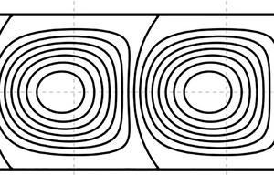
The flow pattern in the critical state is illustrated in figure 4 for the typical case at  $Rn = {10^3}$ with
  ${N_g} = 3.34 \times {10^{ - 2}}$. The convection cell occupies the whole layer in a rectangular shape with the centre located at the midline of the channel. The flow patterns for other values of Rn are similar except for the wavelength. Note that the neutral curve tends to be a flat line at a high value of Rn as shown in figure 3(c). This result implies that the onset of instability could be triggered randomly by disturbances in a wide range of wavelength at high nanoparticle concentration. In a word, the presence of gravity settling obviously causes essential changes in the stability characteristics.

Figure 4. The pattern of convection cells in the critical state:  ${k_c} = 0.75$,
  $R{a_c} = 191.58$,
  $Rn = {10^3}$ and
  ${N_g} = 3.34 \times {10^{ - 2}}$ for the case of
  ${d_p} = 12.\textrm{3}\;\textrm{nm}$.
To further manifest the effect of gravity settling, we depict the variations of  $R{a_c}$ and
  ${k_c}$ with Rn in figure 5(a,b), respectively, for the cases of
  ${N_g} = 0$ and 0.0334. The result shows that the values of
  $R{a_c}$ are equal to 1708 as
  $Rn$ reduces to zero for both cases with the same critical wavenumber 3.12 as illustrated in figure 5(b), which are consistent with those of the classical Rayleigh–Bénard problem. For the case
  ${N_g} = 0$ without the gravity settling effect,
  $R{a_c}$ drops rapidly with increasing Rn and approaches zero gradually, as shown by the blue line in figure 5(a). At
  $Rn = 100$, which is equivalent to the condition of
  ${\phi _0} = 0.000369\%$, for example,
  $R{a_c}$ descends to 11.2, which corresponds to the temperature difference of
  $\Delta T\textrm{ = 0}\textrm{.006}\;\textrm{K}$ only. However, the nanoparticle concentration
  ${\phi _0}$ in common nanofluids is generally larger than
  $0.1\,\%$ (i.e. Rn > 27 100). The corresponding
  $R{a_c}$ is less than 0.04, which indicates that the critical temperature difference would be lower than
  $2.2 \times {10^{ - 5}}\;\textrm{K}$. That is, an infinitesimal temperature difference is sufficient to trigger the onset of instability and convection always occurs in the nanofluid layer.

Figure 5. Variation of (a)  $R{a_c}$ and (b)
  ${k_c}$ with Rn in the case of
  ${d_p} = 12.3\;\textrm{nm}$.
This unconditionally unstable characteristic has been explored in previous work (Ruo, Yan & Chang Reference Ruo, Yan and Chang2021). Besides, the corresponding critical wavenumber  ${k_c}$ is also found to approach zero when Rn exceeds 10, as depicted by the blue line in figure 5(b). This result seems to be doubtful because the critical wavelength should not be infinite, although one can argue that infinitely extended plates are considered in the present analysis. This unusual result of course could be eliminated if one considers finite boundaries in the x and/or y direction to constrain the critical wavelength. Nevertheless, the result for an unconditionally unstable system implies the deficiency of the previous model, and it also contradicts the experimental observation (Kumar et al. Reference Kumar, Sharma and Sood2020). In fact, the unconditionally unstable characteristic with zero critical wavenumber may exist in the system of a binary mixture, which has been verified by experimental observations for a water/isopropanol mixture (Lhost & Platten Reference Lhost and Platten1989). The behaviour predicted by Buongiorno's model is shown to be similar to that occurring in the binary fluid because the thermophoretic diffusion of nanoparticles is almost equivalent to the thermal diffusion of solute. However, the migration of nanoparticles is essentially different from the diffusion behaviour of solute in a binary fluid since some slip mechanisms, in addition to thermophoresis, may appear to influence the diffusion of nanoparticles. As in the case
  ${N_g} = 3.34 \times {10^{ - 2}}$ illustrated in figure 5, the gravity settling effect is evidenced as a critical mechanism. It is clear that, once the gravity settling effect is taken into consideration, the phenomenon of an unconditionally unstable system with zero
  ${k_c}$ is removed. As shown by the red line in figure 5(a), the critical Rayleigh number does not approach zero but approaches a finite value of 190.4 eventually with increasing Rn. Hence, the critical temperature difference would not be infinitesimal any more.
It is noted that the parameters  ${N_A}$ and Ra are linked by
  ${\chi _A}$ as written in (3.1). The critical value of
  ${N_A}$ corresponding to the critical Rayleigh number 190.4 at high Rn condition is almost equal to
  ${N_g}$ (i.e.
  ${N_A} \approx 3.34 \times {10^{ - 2}} = {N_g}$), which renders
  $\hat{E} \approx 0$. It seems that the neutral stable state is determined by the condition
  $\hat{E} = 0$ once the parameter Rn is large enough. This phenomenon can be explained as follows. According to (2.19e), the parameter Rn denotes the strength of buoyancy due to the presence of nanoparticles and acts as a destabilizing effect. When Rn is small, the nanoparticle-induced buoyancy is weak and the stability is dominated by the thermal buoyancy, denoted by Ra. Therefore, the neutral stable state can still be maintained at a positive value of
  $\hat{E}$ for small Rn, although
  $\hat{E} > 0$ indicates an unstably stratified nanoparticle concentration at basic state as shown in figure 2. As Rn increases, the particle-induced buoyancy becomes stronger and eventually controls the stability as Rn exceeds
  ${10^4}$. In this case, a small positive value of
  $\hat{E}$ is enough to induce the onset of instability. Consequently, the neutral stable state at high Rn condition can exist only when the parameter
  $\hat{E}$ is sufficiently close to zero, which indicates a uniform distribution of nanoparticle volume fraction across the nanofluid layer as revealed in figure 2.
The variation of critical wavenumber  ${k_c}$ is also quite different from that of the case
  ${N_g} = 0$. As shown in figure 5(b), the
  ${k_c}$ value descends quickly at first, then it reaches a minimum and rises with
  $Rn$ gradually. The minimum
  ${k_c}$ is
  $\textrm{0}\textrm{.49}$ located approximately at
  $Rn = 200$. Apparently, the gravity settling effect introduced in the present model is a crucial stabilizing mechanism to resist the effect of thermophoresis. As a result, the unrealistic stability behaviours predicted previously by the Buongiorno model can be avoided.
3.2. Stability characteristics at larger nanoparticle sizes
In this section we proceed with examining the effect of gravity settling with larger nanoparticle sizes to explore further physical insights into the onset of instability. The first case considered is nanoparticles with diameter  ${d_p} = \textrm{3}0\;\textrm{nm}$. Accordingly, the related parameters can be recalculated by the same procedure: Le ~ 8933,
  ${\chi _A}\sim 2339$ and Ng ~ 0.484. Note that Pr and
  ${\chi _B}$ remain unchanged because they are independent of
  ${d_p}$. The typical neutral curves at small values of Rn for both cases of
  ${N_g} = 0$ and 0.484 are similar to those of the case
  ${d_p} = 12.3\;\textrm{nm}$ as shown in figure 3(a,b). However, in the present case
  ${N_g} = 0.484$, the descent of the neutral curve becomes quite slow after Rn exceeds 1. Particularly, the oscillatory mode is found to emerge and dominate the onset of instability once Rn is large sufficiently.
Figure 6(a) illustrates the transition from the stationary mode to the oscillatory mode by showing three typical neutral curves of Rn. For the neutral curve of Rn = 2000, only the stationary mode is observed and the critical mode occurs at  $R{a_c} = 1133.03$ and
  ${k_c} = 3.3$. As Rn increases further, the neutral curve dips very slowly and the oscillatory mode begins to appear. One can see that the neutral curve of the typical case
  $Rn = {10^4}$ exhibits a bimodal structure, while the stationary mode on the right still prevails over the oscillatory mode on the left and determines the critical state at
  $R{a_c} = 1132.98$ with
  ${k_c} = 4.3$. Such a bimodal neutral curve has never been found previously when the gravity settling effect is ignored. The oscillatory branch continues to dip slowly and extend gradually with increasing Rn. It is found that both stationary and oscillatory modes may have the same stability at about
  $Rn = 1.1 \times {10^4}$. Once Rn exceeds
  $1.1 \times {10^4}$, the critical mode shifts from the stationary mode to the oscillatory mode coincident with a jump of critical wavenumber to a lower value, as indicated on the neutral curve of
  $Rn = {10^5}$. The magnitudes of oscillatory frequency
  $|{{s_i}} |$ corresponding to the oscillatory neutral curves are depicted in figure 6(b). Obviously, the contour of
  $|{{s_i}} |$ rises gradually with increasing Rn. The critical state at
  $Rn = {10^5}$ occurs at
  $R{a_c} = 1132.94$ with
  ${k_c} = 3.25$ and
  $|{s{}_{i,c}} |= \textrm{0}\textrm{.016}$. The flow pattern becomes distorted convection cells propagating in the horizontal direction at the onset of oscillatory mode as illustrated in figure 7.

Figure 6. (a) The variation of neutral curves showing the transition of the critical mode from stationary mode to oscillatory mode at  ${N_g} = 0.484$, and (b) the corresponding curves of oscillatory frequency
  $|{{s_i}} |$. The solid and dashed lines indicate the stationary and oscillatory modes, respectively.

Figure 7. The pattern of oscillatory convection cells in the critical state with  $Rn = {10^5}$,
  $R{a_c} = 1132.94$,
  ${k_c} = 3.25$,
  $|{s{}_{i,c}} |= \textrm{0}\textrm{.016}$ and
  ${N_g} = 0.484$.
For the Rayleigh–Bénard problem of a pure fluid layer, the onset of instability is always dominated by the stationary mode. This condition is quite different once a binary fluid is considered (Gutkowicz-Krusin, Collins & Ross Reference Gutkowicz-Krusin, Collins and Ross1979). It has been found that the interplay between a stabilizing effect and a destabilizing effect in the system often leads to the onset of an oscillatory mode. For a binary mixture of negative Soret coefficient, the thermal diffusion exhibits a stabilizing effect, which tends to drive the denser component to the lower region, and the thermal buoyancy is the destabilizing effect (Lekkerkerker Reference Lekkerkerker and Riste1982). The competition between these two opposing mechanisms causes the occurrence of oscillatory instability once the stabilizing Soret effect is virtually eliminated by the destabilizing effect. Similarly, in the present nanofluid Rayleigh–Bénard system, the gravity settling effect acts as the stabilizing effect and the thermophoretic diffusion is the destabilizing effects. If one considers the destabilizing thermophoresis effect only in the nanofluid model, the flow instability is enhanced and could become an unconditionally unstable system. While if the gravity settling effect is added in the nanoparticle transport model, the unconditionally unstable situation no longer exists and the competition between the effects of gravity settling and thermophoresis also may induce the onset of the oscillatory mode. The present results reveal that when the destabilizing effect is substantially balanced by the stabilizing effect of gravity settling, the critical state would be dominated by oscillatory convection.
The variations of  $R{a_c}$,
  ${k_c}$ and
  $|{{s_i}_{,c}} |$ with Rn are shown in figure 8(a–c) for the case of
  ${N_g} = 0.484$ in which the dashed lines represent the results of the oscillatory mode, and those for the case
  ${N_g} = 0$ in the absence of gravity settling effect are also demonstrated for comparison. It is seen that the stability characteristics for the case
  ${N_g} = 0$ are still similar to those displayed in figure 5. However, for the case
  ${N_g} = 0.484$, the system stability is raised noticeably when the nanoparticle diameter increases. The value of
  $R{a_c}$ also descends with Rn at first, while it soon approaches a constant as Rn > 1 due to the more significant effect of gravity settling and the corresponding
  ${N_A}$ approaches
  ${N_g}$ again. That is, instead of the unconditionally unstable system predicted by the model of
  ${N_g} = 0$, a neutral stable condition could be reached by considering the gravity settling effect at high Rn condition, which occurs at
  $\hat{E} \approx 0$. Note that the onset of instability would be dominated by the oscillatory mode after Rn > 11 800. The shift of critical mode causing the discontinuities of
  ${k_c}$ and
  $|{{s_i}_{,c}} |$ occurs at Rn = 11 789, where
  ${k_c}$ jumps abruptly from 4.43 to 3.25 and
  $|{{s_i}_{,c}} |$ rises suddenly from zero to
  $\textrm{2}\mathrm{.88\ \times 1}{\textrm{0}^{ - 3}}$. Especially, the critical wavenumber
  ${k_c}$ of the oscillatory mode remains invariable while the corresponding
  $|{{s_i}_{,c}} |$ increases continuously with Rn.

Figure 8. Variations of (a)  $R{a_c}$, (b)
  ${k_c}$ and (c)
  $|{{s_{i,c}}} |$ with Rn for both cases of
  ${N_g} = 0$ and 0.484 at
  ${d_p} = \textrm{3}0\;\textrm{nm}$. The dashed lines represent the oscillatory mode.
Since nanoparticles with larger diameter could significantly enhance the nanofluid layer stability, it is interesting to explore whether a nanofluid layer would be more stable than a pure fluid layer when the nanoparticle diameter increases further. Here we consider the case of  ${d_p} = 46\;\textrm{nm}$ and the dependent parameters are Le ~ 13 697,
  ${\chi _A}\sim 1526$ and Ng ~ 1.746. The neutral curves for four typical values of Rn are shown in figure 9(a–d), in which the stationary and oscillatory modes are indicated by the solid and dashed lines, respectively. Note that at Rn = 0 the neutral curve is a stationary mode, which is the same as that of the pure fluid case with
  $R{a_c} = 1708$. However, once Rn increases from zero, the oscillatory neutral curve appears and dominates the onset of instability, as for the typical case
  $Rn = {10^{ - 3}}$ shown in figure 9(a), in which the curve of the oscillatory mode is quite close to but slightly lower than that of the stationary mode. The curve of the oscillatory mode takes place within the range of k between 1.7 and 5.2, while the magnitude of the oscillatory frequency
  $|{{s_i}} |$ is quite small, as shown in figure 10(a).

Figure 9. Neutral curves for four typical values of Rn at  ${N_g} = 1.746$: (a) 0.001, (b) 1.0, (c) 103 and (d) 105. The solid and dashed lines indicate the stationary and oscillatory modes, respectively.

Figure 10. The curves of oscillatory frequency for four typical values of Rn at  ${N_g} = 1.746$: (a) 0.001, (b) 1.0, (c) 103 and (d) 105.
In contrast to the previous two cases of  ${d_p} = 12.3$ and 30 nm, the neutral curves of both stationary and oscillatory modes do not fall but rise gradually with increasing Rn. As illustrated in figure 9(b,c), the curve of the stationary mode ascends more quickly than that of the oscillatory mode, which renders the difference between the minima of both modes more obvious as Rn increases from
  ${10^{ - 3}}$ to
  ${10^3}$. However, once Rn is large enough, as displayed in figure 9(d), the neutral curves of both the oscillatory and stationary modes tend to be flat lines and almost coincide, although the curve of the oscillatory mode is always lower than that of the stationary mode. This characteristic is similar to the instability behaviour observed in figure 3(c). The corresponding magnitude of
  $|{{s_i}} |$ for the oscillatory mode grows simultaneously as shown in figure 10(a–d). This result reveals that gravity settling is an important factor and profoundly affects the flow instability. Once the nanoparticle diameter is large enough, the gravity settling effect prevails over the influence of thermophoresis and makes the system more stable than a pure fluid layer. This instability characteristic also resolves the contradiction qualitatively between the experimental observation (Kumar et al. Reference Kumar, Sharma and Sood2020) and the previous theoretical predictions. It is noted that the oscillatory neutral curve rises and the critical Ra approaches a constant 2663 for all k. That is, at high Rn condition, the onset of instability could be governed by oscillatory modes in a wide range of wavenumber since they almost possess the same stability.
Figure 11(a–c) show the variations of  $R{a_c}$,
  ${k_c}$ and
  $|{{s_i}_{,c}} |$, respectively, with Rn for both cases
  ${N_g} = 0$ and 1.746. The results for
  ${N_g} = 0$ exhibit the same behaviours as shown in figures 5 and 8. However, the stability characteristics for
  ${N_g} = 1.746$ are obviously different from those of the cases
  ${N_g} = 0.0334$ and 0.484 with smaller nanoparticle diameters. Unlike the variations of
  $R{a_c}$ in figures 5(a) and 8(a), the critical Rayleigh number increases monotonically from 1708 and is always dominated by the oscillatory mode. Then it approaches a constant eventually about 2663 after
  $Rn > {10^5}$. Note that the parameter
  $\hat{E}$ is negative initially at low Rn condition in the present case. For example, at Rn = 1, the
  $\hat{E}$ value at the critical state is about
  $- 0.63$ which would result in a stably stratified profile of nanoparticle concentration in the basic state as indicated in figure 2.

Figure 11. Variations of (a)  $R{a_c}$, (b)
  ${k_c}$ and (c) the oscillatory frequency
  $|{{s_i}_{,c}} |$ with
  $Rn$ for the case of
  ${d_p} = \textrm{46}\;\textrm{nm}$. The dashed lines represent the oscillatory mode with non-zero frequency.
Therefore, the stability of the nanofluid layer rises and a higher temperature difference is required to induce the onset of instability. The stabilizing effect is gradually pronounced with increasing Rn and then decays as the gravity settling effect is counteracted by the stronger thermophoretic effect. Finally, the critical Rayleigh number tends to be invariable with Rn and the neutral state is also characterized by the condition of  $\hat{E} \approx 0$. The critical wavenumber
  ${k_c}$ of the oscillatory mode remains almost constant as shown in figure 11(b), in which
  ${k_c}$ increases quite slowly from 3.12 to 3.16 as Rn rises from 0 to 105. The variation of
  $|{{s_i}_{,c}} |$ in figure 11(c) is similar to that of
  $R{a_c}$, where it grows gradually from zero and ultimately approaches a constant 14.67 after
  $Rn > {10^5}$. The flow pattern of the critical oscillatory mode is shown in figure 12, which displays the same shape as that of the stationary mode shown in figure 4. Each cell appears to occupy the whole layer in a rectangular shape while the convection cells are travelling waves at the onset of instability.

Figure 12. The pattern of oscillatory convection cells in the critical state with  $Rn = {10^5}$, Rac = 2648.60, kc = 3.16,
  $|{{s_{i,c}}} |= 14.67$ and Ng = 1.746.
Table 2 lists the data of critical states for some typical values of  $Rn$. For the present case
  ${d_p} = 46\;\textrm{nm}$, it is obvious that a higher temperature difference
  $\Delta T$ is required to trigger the onset of instability when the nanoparticle volume fraction in the nanofluid increases. The effect of gravity settling would be more significant once the nanoparticle diameter increases further. Hence, it should be expected that the temperature difference
  $\Delta T$ should be increased to induce the onset of convection if larger nanoparticles are employed in a nanofluid layer at the same nanoparticle volume fraction. On the other hand, if small-sized nanoparticles are used in the nanofluid layer, the critical temperature difference would be reduced, as revealed in the typical case of
  ${d_p} = \textrm{12}\textrm{.3}\,\textrm{nm}$, in which the minimum critical temperature difference could be merely about 0.1 K. This implies that it is easier for the nanofluid with smaller nanoparticles to result in the occurrence of thermal convection. Therefore, nanoparticles possessing lower gravity settling velocity should be preferred for industrial purposes if the agglomeration effect can be completely removed. For example, the employment of nanotube-based nanofluids was reported to provide a higher heat transfer efficiency in comparison with other kinds of nanofluids (Ding et al. Reference Ding, Alias, Wen and Williams2006; Yazida, Sidik & Yahya Reference Yazida, Sidik and Yahya2017). The present analysis can provide a reasonable explanation for this phenomenon. Because nanoparticles in non-spherical shapes generally possess a higher aspect ratio and encounter a smaller gravity settling velocity, the nanofluid stability would be reduced and thus the heat transfer performance could be enhanced.
Table 2. The critical values for Al2O3/water nanofluid with  ${d_p} = \textrm{46}\;\textrm{nm}$ and
  $H = \textrm{5}\;\textrm{mm}$.

4. Conclusions
We have implemented a linear stability analysis for the Rayleigh–Bénard problem in nanofluids by introducing the gravity settling effect into Buongiorno's model. The analysis is carried out by using parameters based on the Al2O3/water nanofluid. The results correct the unrealistic prediction by the previous model that the system would be unconditionally unstable with infinite critical wavelength. The contradiction between experimental observations and theoretical predictions also can be resolved by taking this crucial effect into consideration, which opens up a novel thought to explore the thermal convection behaviour in nanofluids.
It is found that the gravity settling effect is substantially a stabilizing mechanism to resist the destabilizing effect of thermophoresis. For a prescribed nanoparticle volume fraction, the critical Rayleigh number obtained by considering the gravity settling effect is always higher than that predicted by the previous model ignoring this effect. However, in comparison with the stability of a pure fluid layer, the addition of nanoparticles to a base fluid could hasten or delay the onset of instability, which depends on the nanoparticle diameter. For nanoparticles with smaller diameter, the gravity settling effect is relatively weak and the effect of thermophoresis is more significant to destabilize the nanofluid layer. Hence, the system would be more unstable than the case of a pure fluid layer and result in a critical Rayleigh number less than 1708. In contrast, once the nanoparticle diameter is large enough, the gravity settling effect would be more pronounced and suppress the destabilizing effect of thermophoresis. As a result, the stability of the nanofluid layer would be enhanced and the critical Rayleigh number would rise above 1708.
In particular, oscillatory instability may emerge on the basis of the competition between the destabilizing effect of thermophoresis and the stabilizing effect of gravity settling. When the gravity settling effect is comparable to the thermophoretic diffusion, the oscillatory mode would dominate the onset of instability. It is also noted that the critical Rayleigh number always tends to be a constant if the nanoparticle concentration is sufficiently large in the nanofluid Rayleigh–Bénard system, in which the critical Rayleigh number can be determined by the condition that the parameter  $\hat{E}$ approaches zero.
The present findings could qualitatively explain the experimental observation that the onset of instability is seen to be delayed in the nanofluid Rayleigh–Bénard problem (Kumar, Sharma & Sood Reference Kumar, Sharma and Sood2020). However, their experiments were somewhat rough and imprecise because they neither measured the critical Rayleigh number nor provided details of the experiments, such as the physical properties of the nanoparticles, the concentrations of the nanofluids and the dimensions of the nanofluid layer. They just simply observed that the onset of convection was delayed by the employment of a nanofluid. Nevertheless, their observations still provide an important hint that the nanofluid Rayleigh–Bénard system could not be an unconditionally unstable system and the addition of nanoparticles to the fluid layer may produce a stabilizing effect on the onset of convection.
The temperature difference between the fluid layer and the ambient air also seems too large to satisfy the Boussinesq approximation; while heat convection between the upper surface and the ambient air may cause the temperature on the upper surface to be much higher than the ambient air temperature. Hence, the upper surface temperature may still be close to the bottom plate temperature and the Boussinesq approximation may still be valid in the experiments. Accordingly, the experimental work (Kumar, Sharma & Sood Reference Kumar, Sharma and Sood2020) is still valuable and suggests that Buongiorno's model needs to be re-examined.
The present results have elucidated that the effect of gravity settling is significant and plays an important role in factors affecting the thermal instability characteristics in the nanofluid Rayleigh–Bénard problem. This effect should be included in a model of nanoparticle diffusion and considered in thermal convection problems of nanofluids. Further experimental work in the future would be helpful for the verification of the present theoretical prediction and the understanding of the nanofluid convection mechanism.
Funding
This work is supported by funding from the Ministry of Science and Technology of Taiwan through the grant numbers MOST 108-2218-E-197-002 and 107-2221-E-036-009.
Declaration of interests
The authors report no conflict of interest.


