


1. Introduction
Pulsatile flows are a common phenomenon in a variety of engineering flows, and they are ubiquitous in physiological configurations. The pulsatile flow through tubular geometries plays a key role in the haemodynamic system of many species as it is responsible for the transport of oxygenated blood to the organs and muscular tissue (Ku Reference Ku1997; Pedley Reference Pedley2000). While in many of these configurations inertial effects are too weak to cause and sustain turbulent fluid motion, a variety of cardiovascular diseases can be linked to flow instabilities in the arteries (Chiu & Chien Reference Chiu and Chien2011). In addition, geometric modifications of the standard fluid-carrying vessels, such as stenoses, aneurysms or other pathologies, further amplify adverse flow effects and aggravate physiological consequences. For these reasons, a better understanding of pulsatile flows, and the perturbation dynamics they support, would be beneficial, if not mandatory, for improved diagnostics as well as the design of advanced medical devices.
Despite their importance in medical and engineering applications, pulsatile flows – and in particular their stability characteristics – have received far less attention than their steady analogues. Pulsatile flows comprise a steady as well as a time-periodic component. This is in contrast to oscillatory flows which consist of a harmonic part, but lack a steady background flow. The periodic time dependence precludes a standard modal approach, based on temporal Fourier normal modes, and instead calls for more complex methods, such as Floquet analysis. Furthermore, pulsatile flows are governed by a far larger suite of parameters than steady flows: besides the common Reynolds number  $Re$ and the wavenumbers of the perturbations, pulsatile flows depend on the pulsation amplitudes and the non-dimensional frequency (the Womersley number
  $Wo$). For a non-modal analysis, the time horizon over which growth or decay is measured and the phase shift of the perturbation within a base-flow cycle have to be accounted for as well. Within this high-dimensional parameter space, a rich and varied perturbation dynamics can be observed, with important transitions between distinct flow behaviours.
The stability of pulsatile flow has been addressed by a few key studies that laid the foundation for our current understanding of its perturbation dynamics. An account of the pertinent body of literature has been presented in Pier & Schmid (Reference Pier and Schmid2017) with emphasis on the modal treatment via Floquet analysis. A resume of earlier work on general time-periodic flows has been presented in Davis (Reference Davis1976). Further notable work by von Kerczek (Reference von Kerczek1982) has built on this foundation and established a framework for the analysis of flows with a harmonic base flow. Generic configurations such as a Stokes layer (Blennerhassett & Bassom Reference Blennerhassett and Bassom2002) or channel and pipe flow with time-periodic pressure gradients (Thomas et al. Reference Thomas, Bassom, Blennerhassett and Davies2011), have been investigated with modal techniques and have been mapped out as to their stability characteristics across a range of governing parameters. The influence of wall modifications, such as stenoses or aneurysms, on the overall stability behaviour has been addressed via numerical simulations (see, e.g. Blackburn, Sherwin & Barkley Reference Blackburn, Sherwin and Barkley2008; Gopalakrishnan, Pier & Biesheuvel Reference Gopalakrishnan, Pier and Biesheuvel2014).
The role of pulsation in the transition from laminar to turbulent pipe flow has been recently investigated by Xu et al. (Reference Xu, Warnecke, Song, Ma and Hof2017) and Xu & Avila (Reference Xu and Avila2018). These studies in particular concentrated on the emergence and life cycle of localised ‘puffs’, together with their role in triggering transition in the presence of a pulsating flow component, since the occurrence of turbulent bursts in each cycle has been found to be sensitive on flow parameters and configuration details. A strong influence of the Womersley number has been reported, and a distinct regime-switching across three proposed parameter regions has been observed (Xu et al. Reference Xu, Warnecke, Song, Ma and Hof2017). These experimental findings have been further corroborated by direct numerical simulations initiated by a localised perturbation (Xu & Avila Reference Xu and Avila2018). The earlier numerical study by Tuzi & Blondeaux (Reference Tuzi and Blondeaux2008) concluded that at moderate but subcritical Reynolds numbers only parts of the harmonic cycle (around flow reversal) support turbulent flow via an instability and an associated break of the flow's symmetry.
While the early body of literature on time-periodic flows has concentrated on a modal (Floquet) approach, more recent studies have employed an initial-value perspective on the analysis of perturbation dynamics and energy growth. Biau (Reference Biau2016) has analysed the generic oscillatory Stokes layer as to its potential to support transiently growing perturbations over a forcing cycle. This study isolated the Orr mechanism as the dominant process by which energy amplification could be achieved efficiently for sufficiently high unsteady amplitudes. In particular the decelerating part of the forcing cycle has been identified as prone to strong non-modal growth. Complementary nonlinear simulations further verified that triggering by these mechanisms can yield subcritical transition to turbulence. A similar technique has been applied in a recent study by Xu, Song & Avila (Reference Xu, Song and Avila2021) for oscillatory and pulsating pipe flow. Among others, they have reported that pulsating pipe flows are generally dominated by helical perturbations. In accordance with Biau (Reference Biau2016), a strong Orr-type mechanism has been found to dominate, once a threshold pulsation amplitude has been exceeded. Again, only half of the forcing cycle supported growth of the kinetic perturbation energy; disturbances have been observed to rapidly reach energy levels that facilitate a transition to turbulent fluid motion, often via localised disturbances.
These latter studies advocate the treatment of pulsatile flow as a generally time-dependent flow, distinct from a periodic Floquet ansatz. Over the past decades, the application of these non-modal techniques to hydrodynamic stability calculations has resulted in a more complete understanding of shear-driven instability phenomena. The generality of this approach (Schmid Reference Schmid2007) is well-suited for assessing pulsatile flow over a range of time scales, thus mapping out the optimal perturbation dynamics over partial and multiple pulsation cycles. This non-modal approach for time-dependent flows is based on a variational principle arising from a partial-differential-equation-constrained optimisation problem. It results in a direct–adjoint system of equations (Luchini & Bottaro Reference Luchini and Bottaro2014) that produce the maximum energy growth of perturbations over a prescribed time horizon. Time-dependent base flows are treated naturally within this formalism, and short-term energy amplification mechanisms, for example over a partial pulsation cycle, can be detected and extracted effectively. Over the past years, this computational framework has been successfully brought to bear on a variety of complex flow configurations (see, e.g. Magri (Reference Magri2019) and Qadri et al. (Reference Qadri, Magri, Ihme and Schmid2021) for applications in reactive flows), and has furnished quantitative stability measures beyond the time-asymptotic limit and without the need for simplifying assumptions.
This article follows up on and extends earlier work (Pier & Schmid Reference Pier and Schmid2017) that demonstrated the influence of a pulsating flow component on the stability of channel flow via a linear (Floquet) and nonlinear analysis. In this present study, we focus on non-modal effects and the occurrence of transient energy amplification mechanisms under conditions that are asymptotically stable, both for rectangular channel and cylindrical pipe flows. The unsteady nature of the base flow lends itself to a formulation as a partial-differential-equation-constrained optimisation problem for the maximum energy gain which is subsequently solved by a variational approach based on direct–adjoint looping.
The main finding, and significance, of our investigation consists of the quantification of extremely large transient growth, brought on by the unsteady nature of the base flow. By considering both channel and pipe flows and carefully studying energy transfer mechanisms, we identify the fundamental mechanisms responsible for this huge growth, common to both geometries. This amplification potential translates directly into a strong sensitivity for the rise of coherent structures over one or many pulsatile cycles. While this feature of pulsatile flows has been observed and reported in previous studies, an encompassing treatment of this phenomenon, including its presence in parameter space and its manifestation in dominant spatial structures, is still missing in the literature on unsteady flows. Our findings also have a direct connection to classifying transition scenarios in wall-bounded flows under the influence of cyclic base flow variations, thus extending the classical scenarios for steady flows and potential routes for the transition to turbulence occurring during part of the cycle.
Despite our attempt to analyse pulsating channel and pipe flows comprehensively, judicious choices had to be made to arrive at an emerging picture for the perturbation dynamics prevailing in these configurations. The ensuing parameter ranges have been selected to capture the most compelling and representative flow phenomena, while limiting our focus to flows encountered in physiological and medical situations. Haemodynamic applications, across a range of blood vessel geometries, are well covered by our choice of parameters. Nonetheless, configurations outside this parameter range are touched upon as well, to establish continuity or bifurcations in flow behaviour and to connect to other studies that investigate such parameter regimes in more detail, e.g. Xu et al. (Reference Xu, Song and Avila2021).
The present paper represents the culmination of several years of work; a preliminary version of the main results has been presented at the 12th European Fluid Mechanics Conference in Vienna (Pier & Schmid Reference Pier and Schmid2018).
2. Flow configurations and governing equations
This investigation considers viscous incompressible flow through infinite channels and pipes of constant diameter. In this context, a flow is characterised by a velocity vector field  ${{{\boldsymbol u}}}({{{\boldsymbol x}}}, t)$ and a scalar pressure field
  $p({{{\boldsymbol x}}}, t)$ that depend on position
  ${{\boldsymbol x}}$ and time
  $t$ and are governed by the Navier–Stokes equations
 $$\begin{gather} \frac{\partial {{\boldsymbol u}}}{\partial t} +({{\boldsymbol u}}\boldsymbol{\cdot} \boldsymbol{\nabla} ) {{\boldsymbol u}} = \nu {\rm \Delta} {{\boldsymbol u}} -\boldsymbol{\nabla} p, \end{gather}$$
 $$\begin{gather}0 = \boldsymbol{\nabla} \boldsymbol{\cdot} {{\boldsymbol u}}, \end{gather}$$
where  $\nu$ is the kinematic viscosity of the fluid, and the pressure has been redefined to eliminate the constant fluid density.
The channel-flow configuration calls for a formulation using Cartesian coordinates, while cylindrical coordinates are appropriate for pipe flows. In order to address both configurations with similar mathematical and numerical tools, we adopt a general formalism using three spatial coordinates  $x_0, x_1, x_2$ and associated velocity components
  $u_0, u_1, u_2$. When analysing channel flow with respect to a Cartesian reference frame, the variables
  $x_0, x_1$ and
  $x_2$ denote wall-normal, streamwise and spanwise coordinates, respectively, while they stand for radial, streamwise and azimuthal coordinates when studying pipe flow in a cylindrical setting. Whatever the configuration, the flow domain corresponds to
  $|x_0|< D/2$ where
  $D$ is the channel or the pipe diameter, and no-slip boundary conditions prevail along the solid walls at
  $|x_0|=D/2$.
A formulation of the incompressible Navier–Stokes equations ((2.1) and (2.2)) in cylindrical coordinates comprises more terms than one in Cartesian coordinates. Nevertheless, the resulting equations have a very similar structure, and the above notations allow us to cast the governing equations into a single general system of partial differential equations, pertaining to both channel and pipe configurations, the details of which are given in Appendix A.
3. Base flows and non-dimensional control parameters
Pulsatile base flows driven by a spatially uniform and temporally periodic streamwise pressure gradient are obtained as exact solutions of the Navier–Stokes equations and consist of a velocity field in the streamwise  $x_1$-direction with profiles that only depend on time
  $t$ and on the wall-normal/radial coordinate
  $x_0$. Denoting by
  $\varOmega$ the pulsation frequency, the base velocity profiles may be expanded as temporal Fourier series,
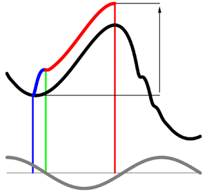
 \begin{equation} U_1(x_0,t) =\sum_n U_1^{(n)}(x_0)\exp({{\mathrm i}}n\varOmega t),\end{equation}
and are associated with a periodic flow rate
 \begin{equation} Q(t)=\sum_n Q^{(n)} \exp ({{\mathrm i}}n\varOmega t). \end{equation}
In the above expressions, the conditions  $Q^{(-n)}=[Q^{(n)}]^{\star }$ and
  $U_1^{(-n)}(x_0)=[U_1^{(n)}(x_0)]^{\star }$ ensure that all flow quantities are real (with
  $\star$ denoting a complex conjugate).
By invariance of these base flows in the streamwise  $x_1$-direction, the different harmonics in the expansion (3.1) are not coupled through the nonlinear terms of the Navier–Stokes equations and the velocity components
  $U_1^{(n)}(x_0)$ are analytically obtained by solving simple differential equations derived for each harmonic component. The mean-flow component
  $U_1^{(0)}(x_0)$ displays a parabolic Poiseuille profile. For
  $n\neq 0$, following Womersley (Reference Womersley1955), the profiles
  $U_1^{(n)}(x_0)$ are obtained in terms of Bessel functions in cylindrical coordinates corresponding to pipe flows, while they are obtained in terms of exponential functions in Cartesian coordinates corresponding to channel flows.
Pulsatile channel or pipe flows are characterised by the Womersley number
 \begin{equation} {Wo}\equiv \frac{D}{2}\sqrt{\frac{\varOmega}{\nu}}, \end{equation}
which is a non-dimensional measure of the pulsation frequency, and may be interpreted as the ratio of the pipe radius (or the channel half-diameter) to the thickness  $\delta =\sqrt {\nu /\varOmega }$ of the oscillating boundary layers developing near the walls. A pulsatile base flow is then completely specified by the Fourier components
  $Q^{(n)}$ of its flow rate (3.2), and the velocity profiles of the different harmonics (3.1) are obtained as
 \begin{equation} U_1^{(n)}(x_0)=\frac{Q^{(n)}}{A} W\left(\frac{x_0}{D/2}, \sqrt{n}{Wo}\right).\end{equation}
In the above expression,  $A$ denotes the relevant measure of the cross-section (
 $A=D$ for channels and
  $A={\rm \pi} D^{2}/4$ for pipes) and the function
  $W$ is the normalised velocity profile pertaining to each harmonic component. The analytic expressions of
  $W$ for channel and pipe flows are given in Appendix B.
In this investigation, we only consider pulsatile flows with a non-vanishing mean flow rate  $Q^{(0)}$. Thus, the definition of the Reynolds number may be based on mean velocity
  $Q^{(0)}/A$, diameter
  $D$ and viscosity
  $\nu$, leading to
 \begin{equation} {Re}\equiv \frac{Q^{(0)}}{\nu}\hbox{ for channels and } {Re}\equiv \frac{Q^{(0)}}{\nu}\frac{4}{{\rm \pi} D}\hbox{ for pipes.}\end{equation}
Moreover, using  $Q^{(0)}$ as reference, the flow rate waveform is completely determined by the non-dimensional ratios
 \begin{equation} \tilde Q^{(n)}\equiv \frac{Q^{(n)}}{Q^{(0)}},\end{equation}
corresponding to the amplitude (and phase) of the oscillating flow rate components ( $n>0$) relative to the mean flow.
In order to reduce the dimensionality of the control-parameter space for the rest of this paper, we will only consider base flow rates with a single oscillating component
 \begin{equation} Q(t)=Q^{(0)}(1+\tilde Q\cos\varOmega t),\end{equation}
where the pulsation amplitude  $\tilde Q\equiv 2\tilde Q^{(1)}$ may be assumed real without loss of generality. Note that the theoretical and numerical methods developed for the present investigation are also suitable for studying the dynamics of pulsating base flows with higher harmonic content.
4. Mathematical formulation
This entire study considers the dynamics of small-amplitude perturbations developing in the basic pulsatile channel and pipe flows specified in the previous section. The incompressible Navier–Stokes equations are, therefore, linearised about these base flows. Considering that the base flows do not depend on the streamwise coordinate  $x_1$ nor on the spanwise/azimuthal coordinate
  $x_2$, infinitesimally small velocity and pressure perturbations may thus be written as spatial normal modes of the form
 $$\begin{gather} {{\boldsymbol u}^{d}}(x_0, t)\exp{{\mathrm i}}(\alpha_1 x_1+\alpha_2 x_2), \end{gather}$$
 $$\begin{gather}{p^{d}}(x_0, t)\exp{{\mathrm i}}(\alpha_1 x_1+\alpha_2 x_2), \end{gather}$$
where  $\alpha _1$ and
  $\alpha _2$ are streamwise and spanwise/azimuthal wavenumbers, respectively. Separation of total flow fields into basic and perturbation quantities and substitution of the expansions (4.1) and (4.2) into the governing equations (2.1) and (2.2) linearised about the relevant time-periodic base flow then yields a system of coupled linear partial differential governing equations of the form
 \begin{equation} {{\boldsymbol A}} \partial_t {{\boldsymbol q}}(x_0,t) = {{\boldsymbol L}}(x_0,t) {{\boldsymbol q}}(x_0,t),\end{equation}
where
 \begin{equation} {{\boldsymbol
q}}(x_0,t)\equiv \begin{pmatrix} u_0^{d}(x_0,t)\\
u_1^{d}(x_0,t)\\ u_2^{d}(x_0,t)\\ p^{d}(x_0,t)
\end{pmatrix} \quad\hbox{and}\quad {{\boldsymbol A}}\equiv
\begin{pmatrix} 1 & 0 & 0 & 0 \\ 0 & 1 & 0 & 0 \\ 0 & 0 & 1
& 0 \\ 0 & 0 & 0 & 0
\end{pmatrix}.\end{equation}
\begin{equation} {{\boldsymbol
q}}(x_0,t)\equiv \begin{pmatrix} u_0^{d}(x_0,t)\\
u_1^{d}(x_0,t)\\ u_2^{d}(x_0,t)\\ p^{d}(x_0,t)
\end{pmatrix} \quad\hbox{and}\quad {{\boldsymbol A}}\equiv
\begin{pmatrix} 1 & 0 & 0 & 0 \\ 0 & 1 & 0 & 0 \\ 0 & 0 & 1
& 0 \\ 0 & 0 & 0 & 0
\end{pmatrix}.\end{equation}
Here, the superscript  $d$ refers to components of the direct problem, to be distinguished from the adjoint variables below (4.6). The spatial differential operator
  ${{\boldsymbol L}}(x_0, t)$ in (4.3) is a 4-by-4 matrix and its coefficients involve
  $\partial _0$-differentiation, depend on the wavenumbers
  $\alpha _1$ and
  $\alpha _2$ as well as on the base velocity profiles
  $U_1(x_0,t)$; see Appendix C for explicit expressions of all these terms.
When studying transient growth effects and searching for optimal initial perturbations that are maximally amplified over a finite-time horizon, it is necessary to choose an appropriate measure of disturbance size (Schmid Reference Schmid2007). Using a classical energy-based inner product, the adjoint governing equations associated with the direct problem (4.3) are routinely obtained as
 \begin{equation} {{\boldsymbol A}} \partial_t {{\boldsymbol q}}^{{\dagger}}(x_0,t) = {{\boldsymbol L}}^{{\dagger}}(x_0,t) {{\boldsymbol q}}^{{\dagger}}(x_0,t),\end{equation}
and the adjoint differential operator  ${{\boldsymbol L}}^{{\dagger} }(x_0, t)$ is explicitly given in Appendix D. In contrast with the direct (4.3), the adjoint equations (4.5) have negative diffusion coefficients and the adjoint fields
 \begin{equation} {{\boldsymbol
q}}^{{\dagger}}(x_0,t)\equiv \begin{pmatrix} u_0^{a}(x_0,t)\\
u_1^{a}(x_0,t)\\ u_2^{a}(x_0,t)\\ p^{a}(x_0,t)
\end{pmatrix},\end{equation}
\begin{equation} {{\boldsymbol
q}}^{{\dagger}}(x_0,t)\equiv \begin{pmatrix} u_0^{a}(x_0,t)\\
u_1^{a}(x_0,t)\\ u_2^{a}(x_0,t)\\ p^{a}(x_0,t)
\end{pmatrix},\end{equation}
are integrated backwards in time.
Denoting by  $\{{{\boldsymbol q}}(x_0, t_i), |x_0|< D/2\}$ an initial perturbation at time
  $t_i$, the evolution of this disturbance at subsequent times
  $t>t_i$ and the associated perturbation energy
  $E(t)$ are then obtained by solving the initial-value problem corresponding to (4.3) with
  ${{\boldsymbol q}}(x_0, t_i)$ specified for
  $|x_0|< D/2$. The temporal evolution of the perturbation amplitude is then characterised by the ratio
  $E(t)/E(t_i)$, for
  $t>t_i$.
The maximum possible amplification of a disturbance over the interval  $t_i< t< t_f$ is obtained as
 \begin{equation} G(t_i,t_f) = \max_{\{{{\boldsymbol q}}(x_0,t_i)\}} \frac{E(t_f)}{E(t_i)},\end{equation}
by optimising over all possible initial conditions at  $t=t_i$. Note that, since the base flow is time-periodic, the amplification factor depends not only on the duration
  $t_f-t_i$ of the temporal evolution but also on the phase of its starting point
  $t_i$ within the pulsation cycle.
The particular initial condition at  $t=t_i$ that achieves the largest amplification at
  $t=t_f$ is referred to as the optimal perturbation and the resulting flow fields at
  $t=t_f$ as the optimal response. In practice, the amplification factors
  $G(t_i,t_f)$ and associated optimal perturbations and responses are iteratively computed by successive direct–adjoint loops, consisting of temporal integration of the direct (4.3) from
  $t_i$ to
  $t_f$ and of the adjoint equations (4.5) from
  $t_f$ to
  $t_i$, using the numerical methods described in the next section.
In linearly stable configurations, all perturbations eventually decay and the maximal transient growth for given wavenumbers  $\alpha _1$ and
  $\alpha _2$,
 \begin{equation} {G^{max}}(\alpha_1,\alpha_2)=\max_{t_i,t_f} G(t_i,t_f; \alpha_1,\alpha_2),\end{equation}
is well defined and takes finite values. Obviously,  ${G^{max}}(\alpha _1,\alpha _2)$ also depends on the base flow configuration and its control parameters. For a given pulsating base flow, the largest possible transient amplification that may be achieved is obtained as
 \begin{equation} {G^{max}_{max}}=\max_{\alpha_1,\alpha_2} {G^{max}}(\alpha_1,\alpha_2),\end{equation}
by considering all possible wavenumbers.
5. Numerical implementation
The direct and adjoint temporal evolution problems (4.3) and (4.5) are first order in time and involve spatial differential operators in the wall-normal  $x_0$-coordinate.
For spatial discretisation we use a Chebyshev spectral method with collocation points spanning the whole diameter of the channel or the pipe. Whether considering channel or pipe flows, all computations are restricted to half of the domain,  $0\leq x_0\leq D/2$, by taking into account the symmetry or antisymmetry of the different flow fields and using the associated discretised differential operators of corresponding symmetry. For channel flow calculations carried out in Cartesian coordinates, the parity of the different flow fields depends on the sinuous or varicose nature of the perturbation under consideration. Note that for all the channel flow configurations considered in this paper, the dynamics is dominated by sinuous perturbations. For pipe flow calculations carried out in cylindrical coordinates, it is the value (even or odd) of the azimuthal mode number that determines the parity of each of the different flow fields. Note that the singularities in the differential operators at the pipe axis (
 $x_0=0$) are only ‘apparent’ (Boyd Reference Boyd2001): the exact solution is analytic at the axis even though the coefficients of the differential equations are not. Thus a consistent implementation of the symmetry/antisymmetry conditions at the axis removes any apparent singularities and guarantees that the spectral method yields smooth solutions.
Time-marching of the direct and adjoint incompressible Navier–Stokes equations uses a second-order accurate predictor–corrector fractional-step method, derived from Raspo et al. (Reference Raspo, Hugues, Serre, Randriamampianina and Bontoux2002). In classical fashion, the maximal gain  $G(t_i,t_f)$, together with optimal initial perturbation and final response, is then obtained by direct–adjoint loops, maximising the energy growth from
  $t=t_i$ to
  $t=t_f$. All subsequent quantities
  ${G^{max}}$ and
  ${G^{max}_{max}}$ are derived from the gain
  $G$, by maximising over
  $t_i$ and
  $t_f$, and over
  $\alpha _1$ and
  $\alpha _2$.
Resorting to the general formulation of the governing equations detailed in the Appendix A and taking advantage of the relevant symmetry properties of the different flow fields thus leads to a numerical implementation capable of handling all configurations of the present investigation.
This entire numerical solution procedure is a generalisation of an approach already used in our previous investigation (Pier & Schmid Reference Pier and Schmid2017), and its implementation in C++ is based on the ‘home-spun’ PackstaB library (Pier Reference Pier2015, § A.6). The interested reader is referred to these references for further details of the general method.
6. Pulsating channel flow
The objective of the present section, which is the core part of the paper, is to investigate how the well known transient-growth properties of steady channel flow are modified by the presence of a pulsating base flow component. Starting with a steady Poiseuille flow, the approach consists of studying the influence of pulsation as the amplitude  $\tilde Q$ is increased from
  $0$ for different values of the Womersley number
  $Wo$.
$Wo$.
First, we consider the growth rates  $G$ of streamwise-invariant and spanwise-periodic streaks since they display the largest transient growth for Poiseuille flow. Then, the strikingly different behaviour observed for two-dimensional (spanwise-invariant) flows calls for a systematic computation of all possible three-dimensional perturbations. Having established the optimal amplification rates
  ${G^{max}}$ that prevail over the whole wavenumber plane, we are then in a position to derive the maximal achievable energy amplification
  ${G^{max}_{max}}$ for a given pulsating base flow and to document its dependence on the pulsation amplitude
  $\tilde Q$, the Womersley number
  $Wo$ and the Reynolds number
  $Re$. Finally, a detailed discussion of the energy transfer mechanisms allows us to highlight the various growth mechanisms that come into play during the different stages of the evolution and to explain the huge growth factors that are observed for pulsating flows, already for moderate pulsation amplitudes. We recall that sinuous perturbations prevail for all the situations investigated here; thus, all the results presented in this section correspond to flow fields of sinuous symmetry.
The vast parameter space of the problem requires a systematic exploration of the flow physics and a concentration on essential characteristics by a progressive compression of the governing parameters. To this end, we successively investigate the growth of streaks, two-dimensional and three-dimensional disturbances, before focusing on transient energy growth and the energy transfer mechanisms that accompany the observed amplifications. We conclude by isolating the shape and dynamics of the two- and three-dimensional structures that optimally exploit the unsteady background flow and thus exhibit maximal energy growth. Along this analysis, we present a sequential reduction of the parameter space, starting from the effect of cycle length and cycle phase, via spatial scales to the time horizon for optimal growth. Within each step, the essential features of the transient instability will be presented, before reducing the parameter dependency for the subsequent analysis. This section then culminates in the detailed examination of the most amplified disturbances, for the two- and three-dimensional case, under the influence of a pulsatile background flow.
6.1. Growth of streaks
In steady channel Poiseuille flow, largest transient growth is known to occur for initial conditions which are spanwise periodic and consist of streamwise aligned vortices, thus corresponding to perturbations with  $\alpha _1=0$ and
  $\alpha _2\neq 0$. Figure 1(a) shows the optimal transient amplification at
  ${Re} =1000, 2000, \ldots , 5000$ computed for
  $\alpha _2=4$, which is near the most transiently amplified spanwise wavenumber. (Throughout this paper, length scales are non-dimensionalised with respect to the channel (or pipe) diameter
  $D$.) For a steady base flow, the energy growth factor
  $G(t_i,t_f)$ only depends on the duration
  $t_f-t_i$, here measured in mean-flow advection units
 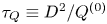 $\tau _Q\equiv D^{2}/Q^{(0)}$. Replotting these data for
  $G/{Re} ^{2}$ and measuring the duration
  $t_f-t_i$ in diffusion units
 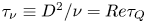 $\tau _\nu \equiv D^{2}/\nu ={Re} \tau _Q$, the curves in figure 1(b) confirm the known scaling laws, leading to a maximum transient growth of
  ${G^{max}}\simeq 1.1 \times 10^{-4}{Re} ^{2}$ at
  $t^{max}/\tau _Q\simeq 1.9 \times 10^{-2}{Re}$.

Figure 1. Optimal energy growth for streaks with  $\alpha _2=4$ and
  $\alpha _1=0$ in steady channel Poiseuille flow at
  ${Re} =1000, 2000$, …,
  $5000$. (a) Duration
  $t_f-t_i$ of growth phase measured in mean-flow advection time scale
  $\tau _Q$. (b) Rescaled growth factors
  $G/{Re} ^{2}$ and
  $t_f-t_i$ measured in diffusion time scale
  $\tau _\nu ={Re} \tau _Q$.
Adding to this steady base flow a pulsatile component of given amplitude and frequency, the transient growth properties are characterised by  $G(t_i,t_f)$ which then depends both on the phase of the initial perturbation
  $t_i$ within the pulsation period
  $T\equiv 2{\rm \pi} /\varOmega$ and on the duration
  $t_f-t_i$ of the temporal evolution. For
  ${Re} =2000$ and
  ${Re} =5000$, figure 2 shows plots of the growth factors
  $G(t_i,t_f)$ for pulsation amplitudes
  $\tilde Q=0.4$ and
  $1.0$ at
  ${Wo} =10$. It is found that the amplitude
  $\tilde Q$ of the base flow modulation only weakly influences the streak growth. Even increasing
  $\tilde Q$ to values larger than unity (corresponding to negative flow rates during part of the pulsation cycle), does not significantly alter the distribution of
  $G(t_i,t_f)$: the maximum amplification remains at the same level and the growth hardly depends on the phase
  $t_i/T$. Thus streamwise-invariant (
 $\alpha _1=0$) perturbations appear to be almost unaffected by the time-dependent component of the base flow and to display a dynamics predominantly dictated by the time-averaged base flow. The discussion of energy transfer mechanisms in § 6.5 below will shed further light on this observation. Comparing figure 2(a) with 2(c), and 2(b) with 2(d), the similarity observed between plots at different
  $Re$ and same
  $\tilde Q$ also indicates that the scaling of
  $G$ with
  ${Re} ^{2}$ remains valid for the transient growth of streaks in pulsating base flows.

Figure 2. Optimal transient amplification for streaks with  $\alpha _2=4$ and
  $\alpha _1=0$ at (a,b)
  ${Re} =2000$ and (c,d)
  ${Re} =5000$. Pulsating channel flow at
  ${Wo} =10$ and (a,c)
  $\tilde Q=0.4$ and (b,d)
  $\tilde Q=1.0$.
6.2. Growth of two-dimensional perturbations
Two-dimensional spanwise invariant perturbations, corresponding to  $\alpha _2=0$ and
  $\alpha _1\neq 0$, exhibit much weaker transient amplification than streaks for the same steady Poiseuille flow. Figure 3 plots the transient growth properties prevailing for Poiseuille flow at
  ${Re} =1000, 2000$, …,
  $5000$ for perturbations with
  $\alpha _1=2$ and
  $\alpha _2=0$, near the most unstable two-dimensional perturbation. Here, the maximal amplification
  ${G^{max}}$ scales linearly with the Reynolds number and reaches much lower values than those corresponding to streaks (see figure 1a); note that this maximal amplification is also reached for a much shorter time horizon.

Figure 3. Optimal energy growth for two-dimensional perturbations  $\alpha _1=2$ and
  $\alpha _2=0$ in channel Poiseuille flow at
  ${Re} =1000, 2000$, …,
  $5000$.
The evolution of two-dimensional transient growth properties as the amplitude  $\tilde Q$ of the pulsating component is increased is given in figure 4. After increasing
  $\tilde Q$, a second maximum emerges in the plot of
  $G$, located around
  $t_i/T=0.2$ and
 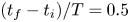 $(t_f-t_i)/T=0.5$. In contrast with the situation prevailing for streaks, this second maximum is seen to rapidly grow with
  $\tilde Q$ and to become the dominant feature, here already for
  $\tilde Q\simeq 0.1$. While streaks display much larger transient growth for steady Poiseuille flow, these two-dimensional perturbations are found to become the most efficient optimal perturbations for pulsatile base flows, beyond some threshold value of the pulsating amplitude
  $\tilde Q$. This overwhelming growth of two-dimensional perturbations for pulsatile conditions will be explained in § 6.5, below, by detailed monitoring of the amplification process in comparison with the dynamics of temporal Floquet eigenmodes.

Figure 4. Optimal transient amplification for two-dimensional perturbations with  $\alpha _2=0$ and
  $\alpha _1=2$ at (a–c)
  ${Re} =2000$ and (d–f)
  ${Re} =5000$. Pulsating base flow at
  ${Wo} =10$ and (a,d)
  $\tilde Q=0.04$, (b,e)
  $\tilde Q=0.10$ and (c,f)
  $\tilde Q=0.20$.
6.3. Growth of three-dimensional perturbations
The very different transient growth behaviour observed for streaky and two-dimensional perturbations calls for a systematic investigation in the entire  $(\alpha _1,\alpha _2)$-wavenumber plane. For a given pulsating base flow, the optimal energy amplification
  ${G^{max}}(\alpha _1,\alpha _2)$ (4.8) is obtained by maximising the transient growth
  $G(t_i,t_f;\alpha _1,\alpha _2)$ over all values of
  $t_i$ and
  $t_f$ at each prescribed wavenumber. We have systematically explored the control-parameter space spanning the ranges
  $1000\leq {Re} \leq 5000, 5\leq {Wo} \leq 15$ and
  $0\leq \tilde Q\leq 1$, and a few characteristic results are presented below.
The plot of  ${G^{max}}$ for steady Poiseuille flow (
 $\tilde Q=0$) at
  ${Re} =4000$ (figure 5a) confirms that strongest transient growth occurs for streaks (with
  $\alpha _1=0$) and that the largest value of
  ${G^{max}}\simeq 1763$ is reached at
  $\alpha _2\simeq 4.09$ (indicated by a black dot). Two-dimensional perturbations (with
  $\alpha _2=0$) experience growth factors that are two orders of magnitude smaller, with
  ${G^{max}}\simeq 30$ for
  $\alpha _1=3.1$.

Figure 5. Isolines of maximum energy growth  ${G^{max}}$ in
  $(\alpha _1,\alpha _2)$-wavenumber plane for base flows with
  ${Re} =4000$ (a–g) and
  ${Re} =2000$ (h–j). (a,h) Steady Poiseuille flow (
 $\tilde Q=0$), (b,d,f,i) pulsating base flows with
  $\tilde Q=0.2$, (c,e,g,j) pulsating base flows with
  $\tilde Q=0.5$. Womersley numbers:
  ${Wo} =8$ in panels (b,c),
  ${Wo} =10$ in panels (d,e,i,j),
  ${Wo} =12$ in panels (f,g). The black dots indicate the wavenumbers where
  ${G^{max}}$ reaches its largest value.
The distribution of maximal amplification factors  ${G^{max}}$ in the
  $(\alpha _1,\alpha _2)$-plane evolves significantly as the amplitude
  $\tilde Q$ of the pulsating component is increased for a given pulsation frequency. Figure 5(b–g) reveal that, as
  $\tilde Q$ is increased, the maximum energy growth (indicated by a black dot) rapidly switches over from streaks to two-dimensional perturbations that experience growth factors sharply increasing with
  $\tilde Q$ while those experienced by streaks (along the
  $\alpha _2$-axis) do not much depend on
  $\tilde Q$ nor on
  $Wo$. Comparison of the results obtained with
  ${Wo} =8$ (figure 5b,c),
  ${Wo} =10$ (figure 5d,e) and
  ${Wo} =12$ (figure 5f,g) demonstrates that the rate of increase of
  ${G^{max}}$ with
  $\tilde Q$ varies significantly with
  $Wo$ and is larger for lower values of the Womersley number.
Figures 5(h–j) illustrate the behaviour at  ${Re} =2000$. For steady Poiseuille flow (figure 5h), the isolines of
  ${G^{max}}$ display a similar structure as for
  ${Re} =4000$ (figure 5a) but with lower levels. After increasing the amplitude
  $\tilde Q$ of the pulsating flow component at
  ${Wo} =10$, figures 5(i,j) show that two-dimensional perturbations again eventually dominate the response. However, at this lower Reynolds number, a larger value of
  $\tilde Q$ is required for the two-dimensional perturbations to emerge, and the increase of
  ${G^{max}}$ with
  $\tilde Q$ also occurs at a lower rate. Thus
  ${G^{max}}$ is found to reach values of the order of
  $10^{5}$ at
  ${Re} =2000$ for
  $\tilde Q=0.5$ and
  ${Wo} =10$ (figure 5j), while at
  ${Re} =4000$ values in excess of
  $10^{11}$ are observed (figure 5e).
6.4. Maximal transient growth
The maximal transient energy amplification achievable for a given base flow has been defined as  ${G^{max}_{max}}$ (4.9) and is derived by maximising
  ${G^{max}}(\alpha _1,\alpha _2)$ over the entire wavenumber plane.
Figure 6 plots the evolution of  ${G^{max}_{max}}$ as the pulsation amplitude
  $\tilde Q$ is continuously increased for Womersley and Reynolds numbers in the range
  $5\leq {Wo} \leq 15$ and
  $1000\leq {Re} \leq 5000$, respectively. At low values of
  $\tilde Q$, the pulsating flow component has a very weak influence and
  ${G^{max}_{max}}$ remains near the value prevailing for steady Poiseuille flow at the same Reynolds number. For these low pulsation amplitudes, the optimal initial perturbation corresponds to streaks (with
  $\alpha _1=0$) and the associated growth duration
  $t_f-t_i$ remains very close to that prevailing for the equivalent mean Poiseuille flow (see also figure 8, below).

Figure 6. Evolution of maximal transient energy amplification  ${G^{max}_{max}}$ with
  $\tilde Q$ for
  $5\leq {Wo} \leq 15$ at (a)
  ${Re} =1000$, (b)
  ${Re} =2000$, (c)
  ${Re} =4000$ and (d)
  ${Re} =5000$.
Beyond some critical value of  $\tilde Q$, the amplification factor
  ${G^{max}_{max}}$ starts to increase exponentially with
  $\tilde Q$, as illustrated by the nearly constant slopes in the logarithmic plots of figure 6 (note the different vertical scale used in figure 6a for
  ${Re} =1000$). This critical value
  $\tilde Q_c$ of the pulsation amplitude depends on
  $Wo$ and
  $Re$ as shown in figure 7(a): increasing the Reynolds number is found to promote the two-dimensional perturbations which become the dominant feature already for
  $\tilde Q>0.1$ around
  ${Re} =5000$. For
  $\tilde Q>\tilde Q_c$, the rate of the exponential growth of
  ${G^{max}_{max}}$ with
  $\tilde Q$ corresponds to the slopes seen in figure 6 and significantly increases as the Womersley number decreases. As a result,
  ${G^{max}_{max}}$ rapidly reaches ‘astronomical’ values, several orders of magnitude beyond the amplification rates prevailing for the corresponding steady Poiseuille flows. These exponential rates have been computed as
 \begin{equation} \kappa\equiv \frac{1}{{G^{max}_{max}}}\frac{\partial{G^{max}_{max}}}{\partial\tilde Q},\end{equation}
and their variation with  $Re$ and
  $Wo$ is given in figure 7(b). In this plot the values of
  $\kappa$ have been computed by taking the average over
  $\tilde Q_c<\tilde Q<\tilde Q_c+0.1$, but note that the growth rate remains nearly constant over much larger intervals of
  $\tilde Q$ in the two-dimensional regime. Obviously, the growth rates are enhanced with the Reynolds number and they also significantly increase towards the lower Womersley numbers, corresponding to longer pulsation periods.

Figure 7. (a) Critical values  $\tilde Q_c$ for transition between streaky and two-dimensional maximally amplified perturbations. (b) Exponential growth rate
  $\kappa$ of
  ${G^{max}_{max}}$ with
  $\tilde Q$ in the two-dimensional regime.
The regime change in the transient growth behaviour occurring for  $\tilde Q=\tilde Q_c$ is further illustrated in figure 8 at
  ${Re} =4000$. The evolution with pulsation amplitude
  $\tilde Q$ of the streamwise
  $\alpha _1$ and spanwise
  $\alpha _2$ wavenumbers associated with the maximally amplified optimal perturbations display a sharp transition from streaky (
 $\alpha _1=0, \alpha _2\neq 0$) to two-dimensional (
 $\alpha _1\neq 0, \alpha _2=0$) perturbations. For
  ${Wo} =6$ and
  $8$, the spanwise wavenumber here directly switches from
  $\alpha _2\simeq 4$ to
  $0$. For higher values of
  $Wo$, however, a small range in
  $\tilde Q$ is observed where the maximally amplified perturbations consist of oblique waves with small but finite values of
  $\alpha _2$. This corresponds to configurations where the amplification of two-dimensional perturbations is still in competition with streaks, so that the maximum of
  ${G^{max}}$ in the
  $(\alpha _1,\alpha _2)$-plane occurs slightly off the
  $\alpha _1$-axis, as illustrated by the black dot in figure 5(f) and corresponding dots in figure 8(a,b). It is then only for higher values of
  $\tilde Q$ that purely two-dimensional (
 $\alpha _2=0$) perturbations prevail.

Figure 8. Characterisation of the maximally amplified optimal perturbations as the pulsation amplitude  $\tilde Q$ is increased for
  ${Wo} =6, 8, 10, 12, 14$ at
  ${Re} =4000$. (a) Streamwise wavenumber
  $\alpha _1$, (b) spanwise wavenumber
  $\alpha _2$, (c) duration of transient growth
  $t_f-t_i$ measured in mean-flow advection units
  $\tau _Q$ and (d) in pulsation periods
  $T$.
$T$.
The transition from streaky to two-dimensional maximally amplified perturbations is also accompanied by a significant change in the duration of the growth phase  $t_f-t_i$, shown in figure 8(c) in mean-flow advection units
  $\tau _Q$ and in figure 8(d) in units of the pulsation period
  $T$. These two time scales are associated with different dynamical features and related as
  ${Wo} ^{2} T=({{\rm \pi} }/{2}) {Re} \tau _Q$. At weak pulsation amplitudes
  $\tilde Q$, the duration
  $t_f-t_i$ remains very close to the value prevailing for streaks developing in the equivalent steady Poiseuille flow, here approximately
  $75\tau _Q$ at
  ${Re} =4000$ (compare with figure 1). At higher pulsation amplitudes, when two-dimensional perturbations dominate, maximal amplification occurs over intervals
  $t_f-t_i$ that approximately correspond to half a pulsation period,
  $T/2$. Thus, the transition from streaky to two-dimensional perturbations also coincides with a change in the dynamical time scale: from streak growth essentially dictated by the mean flow to two-dimensional perturbations strongly amplified over half a pulsation cycle.
6.5. Discussion of energy transfer mechanisms
In this final subsection on channel flows, we investigate the energy production and dissipation mechanisms in order to explain the different transient-growth scenarios that have been identified.
Following the notations introduced in § 4, we consider a perturbation of the form
 \begin{equation} {{\boldsymbol
u}}(x_0,t)\exp{{\mathrm i}}(\alpha_1 x_1+\alpha_2
x_2)+\hbox{c.c.} \quad\hbox{with } {{\boldsymbol
u}}(x_0,t)\equiv \begin{pmatrix} u_0(x_0,t)\\ u_1(x_0,t)\\
u_2(x_0,t)
\end{pmatrix},\end{equation}
\begin{equation} {{\boldsymbol
u}}(x_0,t)\exp{{\mathrm i}}(\alpha_1 x_1+\alpha_2
x_2)+\hbox{c.c.} \quad\hbox{with } {{\boldsymbol
u}}(x_0,t)\equiv \begin{pmatrix} u_0(x_0,t)\\ u_1(x_0,t)\\
u_2(x_0,t)
\end{pmatrix},\end{equation}
using a complex-valued three-dimensional velocity vector  ${{\boldsymbol u}}(x_0,t)$. Such a perturbation is associated with an instantaneous kinetic energy per unit volume of
 \begin{equation} E(t)=\frac{1}{D}\int_{{-}D/2}^{{+}D/2} e(x_0,t)\, {{\mathrm d}}x_0, \end{equation}
where
 \begin{equation} e(x_0,t) =\|{{\boldsymbol u}}(x_0,t)||^{2} \equiv {{\boldsymbol u}}(x_0,t)\boldsymbol{\cdot} [{{\boldsymbol u}}(x_0,t)]^{{\star}},\end{equation}
represents the local energy density. Thus, the temporal energy variation,
 \begin{equation} \frac{{{\mathrm d}}E(t)}{{{\mathrm d}}t}= \frac{1}{D}\int_{{-}D/2}^{{+}D/2} ( \partial_t{{\boldsymbol u}}(x_0,t)\boldsymbol{\cdot} [{{\boldsymbol u}}(x_0,t)]^{{\star}} + {{\boldsymbol u}}(x_0,t)\boldsymbol{\cdot} [\partial_t{{\boldsymbol u}}(x_0,t)]^{{\star}} ) \,{{\mathrm d}}x_0,\end{equation}
follows from the dynamics of  ${{\boldsymbol u}}(x_0,t)$, governed by the Navier–Stokes equations linearised about the pulsating base flow (4.3). Separating terms due to interaction with the base flow from those involving viscous dissipation leads to
 \begin{equation} \frac{{{\mathrm d}}E(t)}{{{\mathrm d}}t}= \varPi(t)-\varTheta(t), \end{equation}
where
 \begin{equation} \varPi(t)= \frac{1}{D}\int_{{-}D/2}^{{+}D/2} {\rm \pi}(x_0,t)\,{{\mathrm d}}x_0 \quad\hbox{and}\quad \varTheta(t)= \frac{1}{D}\int_{{-}D/2}^{{+}D/2} \theta(x_0,t)\, {{\mathrm d}}x_0, \end{equation}
with
 \begin{equation} {\rm \pi}(x_0,t) ={-}\frac{\partial U_1(x_0,t)}{\partial x_0} ( u_0(x_0,t) [u_1(x_0,t)]^{{\star}} + [u_0(x_0,t)]^{{\star}} u_1(x_0,t) )\end{equation}
and
 \begin{equation} \theta(x_0,t) = 2\nu ( \|\partial_0{{\boldsymbol u}}(x_0,t)\|^{2} + (\alpha_1^{2}+\alpha_2^{2})\|{{\boldsymbol u}}(x_0,t)\|^{2} ).\end{equation}
The term  ${\rm \pi} (x_0,t)$ accounts for energy transfer between the pulsating base flow and the perturbation: it essentially represents energy production due to base-flow shear, but negative values may occur and its profile across the channel crucially depends on the relative phases of
  $u_0(x_0,t)$ and
  $u_1(x_0,t)$.
Another quantity of interest is the instantaneous growth rate
 \begin{equation} \sigma(t)\equiv \frac{1}{2E(t)}\frac{{{\mathrm d}}E(t)}{{{\mathrm d}}t} = \frac{\varPi(t) - \varTheta(t)}{2E(t)},\end{equation}
particularly relevant during phases of near-exponential amplification.
Close monitoring of the spatiotemporal development of the base-flow interaction  ${\rm \pi} (x_0,t)$ and the dissipation
  $\theta (x_0,t)$ terms will clarify the amplification mechanisms that govern the different stages of the dynamics.
We focus on two characteristic configurations that have already been discussed: pulsating base flows at  ${Re} =4000$ and
  ${Wo} =10$ with two different pulsation amplitudes,
  $\tilde Q=0.1$ and
  $\tilde Q=0.2$, associated with streaky and two-dimensional maximally amplified perturbations, respectively.
6.5.1. Streaky maximally amplified optimal perturbation
For the lower pulsation amplitude of  $\tilde Q=0.1$, a maximal amplification of
  ${G^{max}_{max}}= 1.77 \times 10^{3}$ is achieved from
  $t_i=0.166T$ to
  $t_f=1.389T$ for streamwise invariant and spanwise periodic perturbations with
  $\alpha _1=0$ and
  $\alpha _2=4.073$. The associated temporal evolution of the perturbation energy
  $E(t)$ is shown in figure 9(a), with the corresponding instantaneous growth rate
  $\sigma (t)$ in figure 9(b). Here, the transient growth is seen to follow the classical pattern prevailing for steady Poiseuille flow: a strong and very short initial boost for
  $t_i< t< t_\star =0.175T$ (blue parts of the curves), followed by a phase of gradually weakening growth for
  $t_\star < t< t_f$ (in red) towards the maximum response. And indeed, these curves in figure 9(a,b) are almost identical to the accompanying insets that correspond to the maximally amplified perturbations for steady Poiseuille flow at the same Reynolds number, characterised by
  $\alpha _1=0, \alpha _2=4.088, {G^{max}_{max}}=1.76 \times 10^{3}$. This evolution is the result of energy production
  $\varPi (t)$ and dissipation
  $\varTheta (t)$, shown in figure 9(c). As can be seen by plotting these quantities relative to the instantaneous energy in figure 9(d), viscous dissipation plays here a minor part in the transient growth throughout the entire process from
  $t_i$ to
  $t_f$.

Figure 9. Temporal development of maximally amplified perturbation at  ${Re} =4000, {Wo} =10$ and
  $\tilde Q=0.1$. Optimal perturbation is streamwise invariant with
  $\alpha _1=0$ and
  $\alpha _2=4.073$. (a) Evolution of energy
  $E(t)$ from
  $t_i=0.166T$ to
  $t_f=1.389T$, leading to
  ${G^{max}_{max}}=1.77\times 10^{3}$. (b) Corresponding instantaneous growth rate
  $\sigma (t)$. (c) Energy production
  $\varPi (t)$ (solid line) and dissipation
  $\varTheta (t)$ (dashed line). (d) Production and dissipation terms relative to instantaneous energy. Insets in panels (a) and (b) correspond to maximally amplified streaks for steady Poiseuille flow at same Reynolds number.
The temporal evolution of the spatial structure of the maximally amplified streaky perturbation is illustrated in figure 10. Selected snapshots correspond to the thick black dots in figure 9:  $t_i=0.166T$ optimal initial perturbation (thick blue curves);
  $t=0.169T$ (thin blue curves);
  $t_\star =0.175T$ at maximal instantaneous growth (thick green curves);
  $t=0.500T$ (thin red curves);
  $t_f=1.389T$ optimal response (thick red curves). In order to enable comparison of these profiles throughout the temporal evolution, they have here all been normalised to unit total energy. As expected, the initial perturbation consists in streamwise aligned vortices, that fill the entire channel cross-section, with a vanishing streamwise velocity component: see thick blue curves in figure 10(a–c) and corresponding vector plot in figure 10(e). Transient amplification promotes streamwise velocity while reducing wall-normal and spanwise velocity components, leading to a final response that solely consists of streamwise velocity: see thick red curves in figure 10(a–c) and
  $u_1$-isolines in figure 10(f). The energy production profiles
  ${\rm \pi}$ shown in figure 10(d) result from the interaction of base flow shear with
  $u_0$ and
  $u_1$, and are therefore significant only around
  $t_\star =0.175T$ (green curve), while displaying vanishing levels near
  $t_i$ and
  $t_f$. Dissipation profiles
  $\theta$ (not shown) remain at small values throughout the entire evolution.

Figure 10. Evolution of spatial structure of maximally amplified streaks for  ${Re} =4000, {Wo} =10$ and
  $\tilde Q=0.1$. Spatial profiles of flow fields (normalised to unit total energy) over half-channel
  $0\leq x_0\leq D/2$ at different snapshots:
  $t_i=0.166T$ optimal initial perturbation (thick blue lines);
  $t=0.169T$ (thin blue lines);
  $t_\star =0.175T$ at maximum growth rate (thick green lines);
  $t=0.500T$ (thin red lines);
  $t_f=1.389T$ optimal response (thick red lines). Envelope of (a) wall-normal
  $|u_0(x_0,t)|$, (b) streamwise
  $|u_1(x_0,t)|$ and (c) spanwise
  $|u_2(x_0,t)|$ velocity perturbations. (d) Energy production
  ${\rm \pi} (x_0,t)$ terms. Snapshots of velocity fields in half-channel over two spanwise wavelengths (
 $\lambda _2=2{\rm \pi} /\alpha _2$): (e) vector plot of
  $(u_0,u_2)$ for initial perturbation at
  $t_i$ and (f) equispaced isolines of streamwise component
  $u_1$ of response at
  $t=t_f$.
Clearly, in this regime, the oscillating component of the base flow has a very weak influence, the amplification process operates as for the equivalent steady Poiseuille flow by redistributing streamwise momentum by streamwise vortices, and the dynamics is essentially dictated by the lift-up effect. This insensitivity to the pulsating base-flow component explains why the maximal growth factors  ${G^{max}_{max}}$ prevailing for streaky optimal perturbations remain at nearly constant level as
  $\tilde Q$ is increased, as observed in figure 6.
6.5.2. Two-dimensional maximally amplified optimal perturbation
A markedly different scenario prevails at higher pulsation amplitudes when the largest transient amplification is achieved for two-dimensional (streamwise periodic and spanwise invariant) perturbations.
As already shown in figure 5(d), for a pulsation amplitude of  $\tilde Q=0.2$, the maximally amplified optimal initial perturbation at
  ${Re} =4000$ and
  ${Wo} =10$ occurs for
  $\alpha _1=2.619$ and
  $\alpha _2=0$ and leads to an amplification of
  ${G^{max}_{max}}=5.48\times 10^{4}$ from
  $t_i=0.168T$ to
  $t_f=0.698T$. The temporal evolution of the perturbation energy is given in figure 11(a), with the associated instantaneous growth rate in figure 11(b). The transient growth that occurs over the interval
  $t_i< t< t_f$ is here seen to develop in two stages: first a relatively short period (phase I, blue curves) of rapid growth followed by a longer interval (phase II, red curves) of weaker but almost constant growth. Between these two stages, the amplification stalls and the instantaneous growth displays a minimum value, which is here slightly negative around
  $t_\star =0.251T$. This two-stage evolution results from production and dissipation contributions, as illustrated in figure 11(c,d): a first peak in
  $\varPi (t)$ during phase I is responsible for the rapid growth of the perturbation, followed by a sustained nearly exponential increase during phase II. The contribution of the relative dissipation
  $\varTheta (t)/2E(t)$ is significant only at the very beginning, before rapidly dropping to low values.

Figure 11. Temporal development of maximally amplified perturbation at  ${Re} =4000, {Wo} =10$ and
  $\tilde Q=0.2$. Optimal perturbation is two-dimensional with
  $\alpha _1=2.619$ and
  $\alpha _2=0$. (a) Evolution of energy
  $E(t)$ from
  $t_i=0.168T$ to
  $t_f=0.698T$, leading to
  ${G^{max}_{max}}=5.48\times 10^{4}$. (b) Corresponding instantaneous growth rate
  $\sigma (t)$. (c) Energy production
  $\varPi (t)$ (solid line) and dissipation
  $\varTheta (t)$ (dashed line). (d) Production and dissipation terms relative to instantaneous energy. Growth occurs in two stages: phase I (in blue) for
  $t_i< t< t_\star$ and phase II (in red) for
  $t_\star < t< t_f$, separated by stall at
  $t_\star =0.251T$ (green vertical line).
The mechanisms responsible for the growth of the perturbation differ in both phases, as illustrated by the profiles in figure 12. These plots show the evolution of the spatial distribution of various fields by selected snapshots, corresponding to the thick black dots in figure 11. Note that the perturbation profiles have again been normalised to unit total energy. The envelopes of wall-normal  $|u_0|$ and streamwise
  $|u_1|$ velocity components in figure 12(a,b) show that the initial perturbation at
  $t_i$ (thick blue curves) is localised toward the wall with maximum amplitude around
  $x_0=0.4D$, before spreading over the entire channel cross-section in the subsequent evolution. The spatial distribution of the base-flow interaction terms
  ${\rm \pi} (x_0,t)$ (shown in figure 12c) reveals that the driving mechanism is strong and concentrated around
  $x_0=0.4D$ in phase I (blue curves) while weaker and evenly spread out in phase II (red curves). In contrast, plots of
  $\theta (x_0,t)$ (figure 12d) show that dissipation is only significant in the initial stages for
  $t\simeq t_i$ and reduced to a very thin boundary layer near the wall throughout the rest of the evolution. The vector plot of the initial perturbation in a streamwise channel cross-section (figure 12e) highlights the flow structures concentrated near the wall and characteristically tilted upstream. In contrast, the final response (figure 12f) fills the entire channel.

Figure 12. Evolution of spatial structure of maximally amplified (two-dimensional) optimal perturbation for  ${Re} =4000, {Wo} =10$ and
  $\tilde Q=0.2$. Spatial profiles of flow fields (normalised to unit total energy) over half-channel
  $0\leq x_0\leq D/2$ at different snapshots:
  $t_i=0.168T$ optimal initial perturbation (thick blue lines);
  $t=0.186T$ and
  $t=0.210T$ in phase I (thin blue lines);
  $t_\star =0.251T$ at stall (thick green lines);
  $t=0.300T$ and
  $t=0.500T$ in phase II (thin red lines); t f = 0.698T optimal response (thick red lines). (a) Envelope of wall-normal
  $|u_0(x_0,t)|$ and (b) streamwise
  $|u_1(x_0,t)|$ velocity perturbations. (c) Energy production
  ${\rm \pi} (x_0,t)$ and (d) dissipation
  $\theta (x_0,t)$ terms. Snapshots of
  $(u_0,u_1)$ velocity fields in half-channel over two streamwise wavelengths (
 $\lambda _1=2{\rm \pi} /\alpha _1$): (e) initial perturbation at
  $t=t_i$ and (f) response at
  $t=t_f$.
Finally, we compare the dynamics of the present maximally amplified optimal perturbation with the development of the temporal normal mode prevailing for the same pulsating base flow at the same spatial wavenumbers. Such normal modes have been extensively computed and characterised in our previous investigation (Pier & Schmid Reference Pier and Schmid2017), using both Floquet eigenproblems and linearised direct numerical simulations.
All pulsatile base flows under consideration here are linearly stable so that temporal eigenmodes decay in the long term. The thick black curve in figure 13 shows the temporal evolution of perturbation energy for the least stable normal mode at  ${Re} =4000, {Wo} =10$ and
  $\tilde Q=0.2$, with
  $\alpha _1=2.619$ and
  $\alpha _2=0$. The negative mean slope in this logarithmic plot confirms the decay, governed by a Floquet multiplier of
  $\mu _F=0.0766$. Thus, the perturbation energy of this normal mode is reduced by a factor of
  $\mu _F^{2}$ after each pulsation period. However, within each pulsation cycle, significant modulation occurs. This intracyclic growth and decay has been shown to approximately coincide with base-flow deceleration and acceleration phases (Pier & Schmid Reference Pier and Schmid2017), as indicated by the grey sinusoidal line representing
  $Q(t)$. Here, the normal mode displays an intracyclic amplification of
  ${G_{nm}}=4.30\times 10^{3}$.

Figure 13. Temporal energy evolution of maximally amplified perturbation (blue and red curves) compared with least stable normal mode (thick black curve), at  ${Re} =4000, {Wo} =10$ and
  $\tilde Q=0.2$, for
  $\alpha _1=2.619$. Normal-mode energy exponentially decays in the long term, according to a Floquet multiplier of
  $\mu _F=0.0766$, but displays intracyclic amplification by a factor of
  ${G_{nm}}=4.30\times 10^{3}$, approximately during half a pulsation period. Optimal perturbation is amplified by
  ${G^{max}_{max}}=5.48\times 10^{4}$. Phase II (in red) closely follows normal mode while phase I (in blue) is very similar to optimal growth prevailing for steady Poiseuille flow at same parameters (inset). Grey sinusoidal curve represents base flow rate
  $Q(t)$ (not to scale).
Comparison of optimal-perturbation and normal-mode energy curves reveals that, during phase II ( $t_\star < t< t_f$, red part of curve in figure 13), the optimal perturbation closely follows the normal-mode dynamics. And, indeed, optimal perturbation and normal mode also display very similar flow fields during that interval.
In the initial phase I ( $t_i< t< t_\star$, blue part of curve in figure 13), however, the maximally amplified perturbation takes advantage of the optimal initial condition responsible for the initial boost in the response through the Orr mechanism. The amplification during phase I is almost identical to the maximal growth experienced by a two-dimensional optimal initial condition for steady Poiseuille flow at the same Reynolds number and same streamwise wavenumber, shown in the inset in figure 13.
These considerations reveal that the maximally amplified two-dimensional perturbation is an optimal combination of Orr mechanism (phase I) and intracyclic normal-mode growth over half a pulsation cycle (phase II). Growth during phase I is essentially determined by the equivalent steady Poiseuille base flow: the resulting amplification factor therefore scales approximately linearly on  $Re$ while being largely independent of
  $Wo$ and
  $\tilde Q$. In contrast, growth during phase II closely follows the intracyclic amplification of the associated temporal eigenmodes, and the magnitude of this intracyclic growth has been shown to strongly depend on
  $Wo$ and
  $\tilde Q$: whatever the Womersley number, it increases almost exponentially with
  $\tilde Q$, and the increase is fastest at the lower values of
  $Wo$ (Pier & Schmid Reference Pier and Schmid2017). This exponential growth with
  $\tilde Q$ explains why two-dimensional optimal perturbations always eventually prevail over streaky perturbations, as observed in figure 6.
The maximal growth factor  ${G^{max}_{max}}$ is obviously always larger than either contribution of phase I or of phase II to the total growth. But while the contribution of phase I remains at moderate levels (one or two orders of magnitude, as for steady Poiseuille flow), it is phase II that is responsible for the huge amplification factors prevailing as the modulation amplitude
  $\tilde Q$ increases. As a result, except for weak pulsation amplitudes, the Orr mechanism only contributes a small factor to the maximal growth
  ${G^{max}_{max}}$, while most of the amplification process is due to modal growth during base-flow deceleration.
7. Pulsating pipe flow
After having presented detailed results for channel flows, we now turn to the transient growth properties of pulsating flows through circular pipes. The organisation of this section is similar to the previous one. However, since most features are equivalent, many details may be omitted here.
By adopting the general formulation appropriate for both Cartesian and cylindrical coordinates, the analysis of pulsating pipe flows is carried out with the same numerical codes as previously used for pulsating channel flows. Due to periodicity in the azimuthal coordinate, the wavenumber  $\alpha _2$ only takes integer values, but otherwise the numerical implementation proceeds as for a Cartesian formulation. Recall that the apparent singularity at the pipe axis (
 $x_0=0$) resolves itself by taking advantage of the symmetry properties relevant for each flow component, since all flow fields are either symmetric or antisymmetric in the radial coordinate
  $x_0$.
7.1. Transient growth of streaks and helical perturbations
Since for steady Hagen–Poiseuille flow, streamwise invariant streaks with  $\alpha _2=1$ and
  $\alpha _1=0$ undergo the largest non-modal growth, we first consider the transient amplification features prevailing for the same type of perturbations developing in pulsating pipe flows. Figure 14 shows the amplification factors
  $G(t_i,t_f)$ obtained at
  ${Wo} =10$, for
  ${Re} =2000$ and
  $5000, \tilde Q=0.4$ and
  $1.0$. The control parameters are the same as those used in figure 2 for pulsating channel flow, and it is observed that the transient growth properties are very similar.

Figure 14. Optimal transient amplification for streaks with  $\alpha _2=1$ and
  $\alpha _1=0$ at (a,b)
  ${Re} =2000$ and (c,d)
  ${Re} =5000$. Pulsating pipe flow at
  ${Wo} =10$ and (a,c)
  $\tilde Q=0.4$ and (b,d)
  $\tilde Q=1.0$.
For streamwise periodic ( $\alpha _1\neq 0$) perturbations, the least stable temporal modes correspond to helical perturbations with
  $\alpha _2=1$. Investigation of transient growth characteristics for
  $\alpha _1\neq 0$ also confirms that perturbations with
  $\alpha _2=1$ dominate over axisymmetric perturbations (
 $\alpha _2=0$) as well as over those of higher azimuthal order (
 $\alpha _2\ge 2$).
Figure 15 illustrates the transient growth properties for  $\alpha _2=1$ and
  $\alpha _1=2$ at
  ${Wo} =10$ and
  ${Re} =2000$ and
  ${Re} =5000$ as the amplitude
  $\tilde Q$ of the pulsating base flow component is increased. As for pulsating channel flow, a second maximum emerges that rapidly dominates the dynamics beyond some value of the base flow modulation amplitude. This maximum is again located near
  $t_i/T=0.2$ and
  $(t_f-t_i)/T=0.5$ and corresponds thus to amplification over half a pulsation cycle.

Figure 15. Optimal transient amplification for helical perturbations with  $\alpha _2=1$ and
  $\alpha _1=2$ at (a–c)
  ${Re} =2000$ and (d–f)
  ${Re} =5000$. Pulsating pipe flow at
  ${Wo} =10$ and (a,d)
  $\tilde Q=0.1$, (b,e)
  $\tilde Q=0.4$ and (c,f)
  $\tilde Q=0.6$.
7.2. Optimal growth at given wavenumbers
The maximal transient growth  ${G^{max}}$, computed by optimisation of
  $G(t_i,t_f)$ over all values of
  $t_i$ and
  $t_f$ for fixed wavenumbers
  $\alpha _1$ and
  $\alpha _2$, is shown in figure 16. In each plot the evolution of
  ${G^{max}}$ curves for
  $0<\alpha _1<6$ is illustrated as
  $\tilde Q$ is increased from
  $\tilde Q=0$ to
  $\tilde Q=1$ in steps of
  $0.1$. Panels (a–c) compare the growth of axisymmetric perturbations,
  $\alpha _2=0$ in panel (a), with that of helical perturbations,
  $\alpha _2=1$ in panel (b) and
  $\alpha _2=2$ in panel (c). Clearly, under pulsating flow conditions, axisymmetric initial conditions undergo transient amplification that is not much larger than for the equivalent steady Poiseuille flow, as demonstrated by the nearly overlapping curves in figure 16(a). Non-axisymmetric perturbations, however, experience transient amplification that rapidly grows with
  $\tilde Q$, and strongest growth occurs for
  $\alpha _2=1$ (figure 16b). Computation of
  ${G^{max}}$ for all
  $\alpha _2\leq 6$ (results not shown) reveals that the same scenario prevails at higher azimuthal order, but the rate of increase of
  ${G^{max}}$ with
  $\tilde Q$ is significantly weaker for higher
  $\alpha _2$.

Figure 16. Maximum energy growth  ${G^{max}}$ for pulsating pipe flows, over
  $0<\alpha _1<6$ at
  $\tilde Q=0.0, 0.1, 0.2$, …,
  $1.0$. Here (a–f)
  ${Re} =4000$ and (g–i)
  ${Re} =2000$; (a–c,h)
  ${Wo} =10$, (d,g)
  ${Wo} =8$, (e)
  ${Wo} =12$ and (f,i)
  ${Wo} =14$; (a)
 $~\alpha _2=0$, (b,d–i)
  $\alpha _2=1$ and (c)
  $\alpha _2=2$.
Evolution of the growth characteristics for  ${Re} =4000$ with different Womersley numbers,
  ${Wo} =8$ in panel (d),
  ${Wo} =12$ in panel (e) and
  ${Wo} =14$ in panel (f), confirms again that largest amplification factors occur for lower pulsation frequencies, i.e., longer pulsation cycles.
Finally, values obtained at lower  ${Re} =2000$ for
  ${Wo} =8$ in panel (g),
  $10$ in panel (h) and
  $14$ in panel (i) show that the general trend is similar but with lower values of
  ${G^{max}}$, as expected for lower
  $Re$.
$Re$.
7.3. Maximal amplification
Finally, the maximal amplification  ${G^{max}_{max}}$ achievable for a given pulsating pipe flow is obtained by optimising
  ${G^{max}}(\alpha _1,\alpha _2)$ over all streamwise wavenumbers
  $\alpha _1$ and azimuthal mode numbers
  $\alpha _2$. Figure 17 shows the variation of
  ${G^{max}_{max}}$ as the pulsation amplitude
  $\tilde Q$ is increased for Womersley numbers in the range
  $5\leq {Wo} \leq 15$ and
  ${Re} =2000, 3000, 4000$ and
  $5000$. The behaviour is again found to be similar to that prevailing for pulsating channel flows: at low pulsation amplitudes,
  ${G^{max}_{max}}$ hardly departs from the value corresponding to the equivalent steady Poiseuille flow; beyond a critical value
  $\tilde Q_c$ of the pulsation amplitude
  $\tilde Q$, transition to approximately exponential growth of
  ${G^{max}_{max}}$ with
  $\tilde Q$ takes over. The results shown in figure 17(a) perfectly match those of figure 4(a) of Xu et al. (Reference Xu, Song and Avila2021), for the subset of control parameter values that is common to both studies. This agreement further validates our methods.

Figure 17. Evolution of maximal transient energy amplification  ${G^{max}_{max}}$ for pulsating pipe flows with
  $\tilde Q$ for
  ${Wo} =5, 6, 7$, …,
  $15$ at (a)
  ${Re} =2000$, (b)
  ${Re} =3000$, (c)
  ${Re} =4000$ and (d)
  ${Re} =5000$.
The variation with  $Wo$ and
  $Re$ of the critical value
  $\tilde Q_c$ for crossover between the two regimes is shown in figure 18(a). In the exponential regime prevailing for
  $\tilde Q\ge \tilde Q_c$, the growth rates
  $\kappa$ corresponding to the slopes in figure 17 are given in figure 18(b), computed according to (6.1). For a given Reynolds number, the curves of
  $\tilde Q_c$ in figure 18(a) are seen to display a minimum for moderate values of the Womersley number, while they increase both for large and small values of
  $Wo$. The increase of
  $\tilde Q_c$ with
  $Wo$ for
  ${Wo} \ge 10$ is strongest at lower values of the Reynolds number. In contrast, for
  ${Wo} \le 10$ the values of
  $\tilde Q_c$ depend much less on
  $Re$.
$Re$.

Figure 18. (a) Critical values  $\tilde Q_c$ for transition between streaky and helical maximally amplified perturbations in pulsating pipe flows. (b) Exponential growth rate
  $\kappa$ of
  ${G^{max}_{max}}$ with
  $\tilde Q$ in the helical regime.
Comparison of the values of  $\tilde Q_c$ and
  $\kappa$ for pipe flows (figure 18) with those prevailing for channel flows shown in figure 7, reveals that pipe flows require larger pulsation amplitudes to switch to the regime with exponentially growing amplification factors
  ${G^{max}_{max}}$. This is especially true for lower Womersley numbers (see also figure 20 below with additional data for
  ${Wo} =3$). Also, while the growth rates
  $\kappa$ display very similar trends for both channel (figure 7b) and pipe configurations (figure 18b), the values for pipe flows are approximately half those of channel flows.
The streamwise wavenumber  $\alpha _1$ associated with the most amplified perturbation as the pulsation amplitude
  $\tilde Q$ is varied for a range of Womersley numbers is monitored in figures 19(a) and 19(b) for
  ${Re} =2000$ and
  $Re=4000$, respectively. These plots demonstrate that the regime change occurring at
  $\tilde Q_c$ is indeed associated with a jump in streamwise wavenumber from
  $\alpha _1=0$ for
  $\tilde Q<\tilde Q_c$ to finite
  $\alpha _1$-values for
  $\tilde Q>\tilde Q_c$. In contrast with channel flows, however, for all pulsating pipe flow configurations investigated here, the optimal perturbations always occur with azimuthal mode number
  $\alpha _2=1$. Thus the critical value
  $\tilde Q_c$ always corresponds to a transition from streaky (
 $\alpha _1=0, \alpha _2=1$) to helical (
 $\alpha _1\neq 0, \alpha _2=1$) optimal perturbations, at the same azimuthal mode number.

Figure 19. Characterisation of the maximally amplified optimal perturbations as the pulsation amplitude  $\tilde Q$ is increased for
 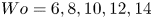 ${Wo} =6, 8, 10, 12, 14$. Streamwise wavenumber
  $\alpha _1$ at (a)
  ${Re} =2000$ and (b)
  ${Re} =4000$. Duration of transient growth
  $t_f-t_i$ at
  ${Re} =4000$ (c) measured in mean-flow advection units
  $\tau _Q$ and (d) in pulsation periods
  $T$.
$T$.
This regime change is also associated with a discontinuity in the duration of the growth phase  $t_f-t_i$ for the optimal amplification process, as illustrated in figure 19(c,d) for
  ${Re} =4000$. The optimised duration
  $t_f-t_i$ is given in mean-flow advection units
  $\tau _Q$ in figure 19(c) and in units of the pulsation period
  $T$ in figure 19(d). These plots illustrate that pulsating pipe flows display similar transient dynamics as channel flows: for
  $\tilde Q<\tilde Q_c$, the optimal duration
  $t_f-t_i$ remains close to the value prevailing for the average parabolic flow profile; for
  $\tilde Q>\tilde Q_c$, when helical perturbations dominate, maximal amplification occurs over intervals corresponding approximately to half a pulsation period. Thus our results confirm the findings of Xu et al. (Reference Xu, Song and Avila2021) that helical perturbations dominate the transient growth at large pulsation amplitudes. By our detailed comparison of channel and pipe configurations at moderate pulsation frequencies, we have been able to highlight the fundamental growth mechanisms, which are common to both geometries.
8. Conclusion
Considering pulsating flows through both channels and pipes, we have investigated the non-modal transient energy amplification resulting from optimal initial conditions. Our study has systematically covered the pulsating base flows for  $1000\leq {Re} \leq 5000, 5\leq {Wo} \leq 15$ and
  $0\leq \tilde Q\leq 1$.
While channel and pipe flows display quite different linear modal stability characteristics, their non-modal transient growth features are found to be very similar in situations that are linearly stable. Optimal energy growth occurs according to two distinct scenarios. At weak pulsation amplitudes  $\tilde Q$, the behaviour is similar to that resulting from the equivalent steady Poiseuille flow, and the oscillating flow component appears to have only a small effect. Beyond a critical value of
  $\tilde Q$, however, transient growth increases exponentially with
  $\tilde Q$ and reaches astronomical values, already for moderate pulsation amplitudes. In this latter regime, optimal growth mainly occurs over half a pulsation period, during the slow part of the pulsation cycle, and closely follows the intracyclic amplification of the associated Floquet eigenmodes. We have previously shown (Pier & Schmid Reference Pier and Schmid2017) that the intracyclic modulation amplitudes derived from temporal normal modes may be huge, even for linearly decaying eigenmodes. The maximal transient amplification factors
  ${G^{max}_{max}}$ computed in the present investigation are even larger since they take advantage of both this normal-mode intracyclic growth and non-modal Orr-type amplification, which contributes in the early stage of the growth process.
These findings have been firmly established by a comprehensive investigation of pulsating flows over the range  $5\leq {Wo} \leq 15$, deemed to be the most relevant for applications in the haemodynamic context. In order to explore the expected behaviour beyond that frequency range, figure 20 shows the maximal achievable transient growth
  ${G^{max}_{max}}$ for channel and pipe flows at
  ${Re} =5000$, extending the results of figures 6(d) and 17(d) by including data at lower and higher pulsation frequencies,
  ${Wo} =3$ and
  ${Wo} =20$, respectively. At high pulsation frequencies, it is observed that the pulsating component is rather inefficient in producing
  ${G^{max}_{max}}$ factors beyond those prevailing for steady base flows, a result closely related to the fact that high-frequency pulsation also has a strong stabilising effect on modal temporal growth rates. In the low frequency regime, the curves for
  ${Wo} =3$ indicate that strong growth is still possible but requires larger pulsation amplitudes
  $\tilde Q$. When lowering
  $Wo$, the critical value
  $\tilde Q_c$ for onset of the exponential regime increases moderately for channel flows and significantly for pipe flows (
 $\tilde Q_c\simeq 0.98$ for
  ${Wo} =3$). These plots are in agreement with observations already made by Xu et al. (Reference Xu, Song and Avila2021) for pulsating pipe flows. Concerning the spatial structure of the optimal perturbations, the results of figure 20 follow the same scenario as previously discussed: while streaky perturbations prevail for
  $\tilde Q<\tilde Q_c$, at larger pulsation amplitudes two-dimensional and helical perturbations dominate, respectively, in channel and pipe flows.

Figure 20. Evolution of maximal transient energy amplification  ${G^{max}_{max}}$ with
  $\tilde Q$ for
 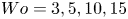 ${Wo} =3, 5, 10, 15$ and
  $20$ at
  ${Re} =5000$, for (a) channel and (b) pipe configurations.
It should be noted that a major difference between channel and pipe flows concerns their linear modal instability features. Indeed, for channel flows there exists a critical Reynolds number beyond which linear instability occurs. This is well known for steady Poiseuille channel flow, and the dependence of this critical Reynolds number with the pulsating flow parameters has been extensively discussed in our previous work (Pier & Schmid Reference Pier and Schmid2017). By contrast, steady pipe Poiseuille flow remains linearly stable, whatever the Reynolds number. For time-periodic base flows, linear instability has been found for purely oscillating pipe flows (Thomas et al. Reference Thomas, Bassom, Blennerhassett and Davies2011). However, the presence of a non-vanishing mean flow rate appears to have a stabilising effect and all pulsating pipe flows considered in the present study are far from temporal instability.
Another difference is that two-dimensional (spanwise invariant and streamwise periodic) perturbations are the most unstable or the least stable for channel flows, whereas the leading linear instability for pipe flows occurs for helical modes with  $\alpha _2=1$ and
  $\alpha _1\neq 0$, which dominate over perturbations of higher azimuthal order (
 $\alpha _2\ge 2$) as well as over axisymmetric (
 $\alpha _2=0$) ones. It is found that this remains true for pulsating pipe flows.
While channel flows are rapidly dominated by two-dimensional sinuous perturbations, pipe flows are dominated by helical perturbations in similar pulsating flow regimes. For pipe flows, axisymmetric perturbations never prevail. But note that the Cartesian equivalent of axisymmetric perturbations are two-dimensional perturbations of varicose symmetry, which never prevail either. The closest equivalent to a two-dimensional sinuous perturbation in a cylindrical geometry is a helical perturbation (with  $\alpha _2=1$).
This study gives a detailed and comprehensive perspective on the perturbation dynamics in pulsatile channel and pipe flow, treating these configurations within a time-dependent, initial-value problem formalism and thus avoiding restrictive assumptions of a modal, time-asymptotic approach. This analysis identified a rich perturbation behaviour driven by parametric and transient excitation over one or multiple forcing cycles and the dominance of an Orr-type amplification mechanism at early times that acts efficiently and selectively across a significant parameter range, once a critical pulsation amplitude has been surpassed.
Our study lays the foundation for a future analysis of pulsating base flows with higher harmonic content, such as blood flow rates resulting from the cardiac pulse. The present approach could also be generalised to take into account compliant walls or to address nonlinear fluid effects.
Acknowledgements
Institut national de physique nucléaire et de physique des particules (IN2P3-CNRS) is warmly thanked for very generously providing computing resources. Without access to its Centre de calcul allowing us to run thousands of independent single-processor jobs, it would have been very difficult to carry out the present research.
Early stages of this work were carried out while B.P. was visiting the BP Institute, enjoying a French Government Fellowship at Churchill College, Cambridge University.
Funding
The Royal Society is gratefully acknowledged for its financial support through an International Exchanges Cost Share award (IEC/R2/170133).
Declaration of interests
The authors report no conflict of interest.
Appendix A. General formulation of the Navier–Stokes equations
In order to handle both Cartesian and cylindrical formulations of the governing Navier–Stokes equations ((2.1) and (2.2)), a general set of spatial coordinates  $x_0, x_1, x_2$ and associated velocity components
  $u_0, u_1, u_2$ is used. These correspond to either wall-normal, streamwise and spanwise directions for channel flows, or radial, streamwise and azimuthal directions for pipe flows, respectively. Using these coordinates and velocity fields, the components of the incompressible Navier–Stokes equations become
 $$\begin{gather} \partial_t u_0 +({{\boldsymbol u}}\boldsymbol{\cdot} \boldsymbol{\nabla} ) u_0 -\boxed{\frac{1}{x_0}u_2^{2}}\phantom{u_2} =\nu \left({\rm \Delta} u_0 +\boxed{\frac{1}{x_0^{2}} \left({-}u_0-2\partial_2 u_2 \right)}\right) -\partial_0 p, \end{gather}$$
 $$\begin{gather}\partial_t u_1 +({{\boldsymbol u}}\boldsymbol{\cdot} \boldsymbol{\nabla} ) u_1 \phantom{{}+\boxed{\frac{1}{x_0}u_0 u_2}} = \nu \left({\rm \Delta} u_1 \phantom{{}+\boxed{\frac{1}{x_0^{2}} \left({-}u_0-2\partial_2 u_2 \right)}} \right) -\partial_1 p, \end{gather}$$
 $$\begin{gather}\partial_t u_2 +({{\boldsymbol u}}\boldsymbol{\cdot} \boldsymbol{\nabla} ) u_2 +\boxed{\frac{1}{x_0}u_0 u_2} = \nu \left({\rm \Delta} u_2 +\boxed{\frac{1}{x_0^{2}} \left({-}u_2+2\partial_2 u_0 \right)} \right) -\boxed{\frac{1}{x_0}} \partial_2 p, \end{gather}$$
 $$\begin{gather}0=\partial_0 u_0 +\boxed{\frac{1}{x_0} u_0} + \partial_1 u_1 + \boxed{\frac{1}{x_0}} \partial_2 u_2, \end{gather}$$
with the notations
 \begin{equation} \partial_0\equiv\partial_{x_0},\quad \partial_1\equiv\partial_{x_1},\quad \partial_2\equiv\partial_{x_2},\end{equation}
and
 $$\begin{gather} {{\boldsymbol u}}\boldsymbol{\cdot} \boldsymbol{\nabla} \equiv u_0\partial_0+ u_1\partial_1 +\boxed{\frac{1}{x_0}} u_2\partial_2, \end{gather}$$
 $$\begin{gather}{\rm \Delta} \equiv \partial_{00} +\boxed{(1/x_0)\partial_0} +\partial_{11} +\boxed{(1/x_0^{2})} \partial_{22}. \end{gather}$$
In these expressions, the terms enclosed in boxes are only present in the formulation using cylindrical coordinates and pertaining to the pipe flow configuration. Resorting to such a general formalism is particularly useful when developing numerical codes to solve both channel and pipe flows: the boxed terms may be switched on or off depending on the flow configuration.
Appendix B. Analytic expressions of the pulsating base flow profiles
For pulsating base flows prevailing in infinite channels or pipes, the harmonic components  $U_1^{(n)}(x_0)$ of the streamwise velocity fields (3.1) display profiles following the shape function
  $W(\xi ,\omega )$ with
  $\xi =2x_0/D$ and
  $\omega =\sqrt {n}{Wo}$.
When considering channel flows in Cartesian coordinates, the oscillating velocity profiles are analytically obtained in terms of hyperbolic functions
 \begin{equation} W(\xi,\omega) \equiv \left. {\left(\frac{\cosh(\sqrt{{{\mathrm i}}}\xi \omega)}{\cosh(\sqrt{{{\mathrm i}}} \omega)} -1\right)} \right/ {\left(\frac{\tanh(\sqrt{{{\mathrm i}}} \omega)}{\sqrt{{{\mathrm i}}} \omega} -1\right)},\end{equation}
for  $|\xi |\leq 1$ and
  $\omega \neq 0$, while the steady component is parabolic,
 \begin{equation} W(\xi,\omega=0)\equiv\tfrac{3}{2}(1-\xi^{2}).\end{equation}
When considering pipe flows in cylindrical coordinates, the velocity profiles involve Bessel functions
 \begin{equation} W(\xi,\omega) \equiv \left. {\left(\frac{J_0(\sqrt{-{{\mathrm i}}}\xi \omega)}{J_0(\sqrt{-{{\mathrm i}}} \omega)} -1\right)} \right/ {\left(\frac{2}{\sqrt{-{{\mathrm i}}}\omega}\frac{J_1(\sqrt{-{{\mathrm i}}} \omega)}{J_0({\sqrt{-{{\mathrm i}}} \omega})} -1\right)}, \end{equation}
with  $J_0$ and
  $J_1$ denoting the classic Bessel functions of the first kind. The steady component is again parabolic,
 \begin{equation} W(\xi,\omega=0)\equiv 2(1-\xi^{2}).\end{equation}
All the profiles above are normalised so that their cross-sectional average equals unity. Thus, the pulsating base flow velocity components (3.4) are simply obtained by multiplying these profiles with the flow rate coefficients  $Q^{(n)}$.
Appendix C. Linear governing equations of direct problem
In the direct formulation of the incompressible Navier–Stokes equations (4.3), the spatial differential operator  ${{\boldsymbol L}}(x_0, t)$ is a 4-by-4 matrix of the form
 \begin{gather} {{\boldsymbol L}}(x_0,t)\equiv \begin{pmatrix} L_{00}(x_0,t) & 0 & L_{02}(x_0,t) & -\partial_0\\ L_{10}(x_0,t) & L_{11}(x_0,t) & 0 & -{{\mathrm i}}\alpha_1 \\ L_{20}(x_0,t) & 0 & L_{22}(x_0,t) & -\boxed{\dfrac{1}{x_0}} {{\mathrm i}}\alpha_2 \\ -\partial_0 -\boxed{\dfrac{1}{x_0}} & -{{\mathrm i}}\alpha_1 & -\boxed{\dfrac{1}{x_0}} {{\mathrm i}}\alpha_2 & 0 \end{pmatrix},\end{gather}
Its coefficients involve  $\partial _0$-differentiation, depend on the spatial wavenumbers as well as on the base flow velocity profiles. Their explicit expressions are the following:
 $$\begin{gather} L_{00}(x_0,t)={-}{{\mathrm i}}\alpha_1 U_1(x_0,t) +\nu \left({\rm \Delta} -\boxed{\frac{1}{x_0^{2}}}\right), \end{gather}$$
 $$\begin{gather}L_{11}(x_0,t)={-}{{\mathrm i}}\alpha_1 U_1(x_0,t) +\nu {\rm \Delta} , \end{gather}$$
 $$\begin{gather}L_{22}(x_0,t)={-}{{\mathrm i}}\alpha_1 U_1(x_0,t) +\nu \left({\rm \Delta} -\boxed{\frac{1}{x_0^{2}}}\right), \end{gather}$$
 $$\begin{gather}L_{10}(x_0,t)={-}\partial_0 U_1(x_0,t), \end{gather}$$
 $$\begin{gather}L_{20}(x_0,t)={-}L_{02}(x_0,t)= \boxed{2\nu \frac{{{\mathrm i}}\alpha_2}{x_0^{2}}}, \end{gather}$$
with
 \begin{equation} {\rm \Delta} \equiv \partial_{00} +\boxed{\frac{1}{x_0}\partial_0} -\alpha_1^{2} -\boxed{\frac{1}{x_0^{2}}} \alpha_2^{2}.\end{equation}
Appendix D. Adjoint problem
In the adjoint formulation of the incompressible Navier–Stokes equations (4.5), the spatial differential operator  ${{\boldsymbol L}}^{{\dagger} }(x_0, t)$ is obtained as
 \begin{equation} {{\boldsymbol
L}}^{{\dagger}}(x_0,t)\equiv \begin{pmatrix}
L_{00}^{{\dagger}}(x_0,t) & L_{01}^{{\dagger}}(x_0,t) &
L_{02}^{{\dagger}}(x_0,t) & -\partial_0\\ 0 &
L_{11}^{{\dagger}}(x_0,t) & 0 & -{{\mathrm i}}\alpha_1 \\
L_{20}^{{\dagger}}(x_0,t) & 0 & L_{22}^{{\dagger}}(x_0,t) &
-\boxed{\dfrac{1}{x_0}} {{\mathrm i}}\alpha_2 \\
-\partial_0 -\boxed{\dfrac{1}{x_0}} & -{{\mathrm
i}}\alpha_1 & -\boxed{\dfrac{1}{x_0}} {{\mathrm i}}\alpha_2
& 0 \end{pmatrix},\end{equation}
\begin{equation} {{\boldsymbol
L}}^{{\dagger}}(x_0,t)\equiv \begin{pmatrix}
L_{00}^{{\dagger}}(x_0,t) & L_{01}^{{\dagger}}(x_0,t) &
L_{02}^{{\dagger}}(x_0,t) & -\partial_0\\ 0 &
L_{11}^{{\dagger}}(x_0,t) & 0 & -{{\mathrm i}}\alpha_1 \\
L_{20}^{{\dagger}}(x_0,t) & 0 & L_{22}^{{\dagger}}(x_0,t) &
-\boxed{\dfrac{1}{x_0}} {{\mathrm i}}\alpha_2 \\
-\partial_0 -\boxed{\dfrac{1}{x_0}} & -{{\mathrm
i}}\alpha_1 & -\boxed{\dfrac{1}{x_0}} {{\mathrm i}}\alpha_2
& 0 \end{pmatrix},\end{equation}
with
 $$\begin{gather} L_{00}^{{\dagger}}(x_0,t)={-}{{\mathrm i}}\alpha_1 U_1(x_0,t) -\nu \left({\rm \Delta} -\boxed{\frac{1}{x_0^{2}}}\right), \end{gather}$$
 $$\begin{gather}L_{11}^{{\dagger}}(x_0,t)={-}{{\mathrm i}}\alpha_1 U_1(x_0,t) -\nu {\rm \Delta} , \end{gather}$$
 $$\begin{gather}L_{22}^{{\dagger}}(x_0,t)={-}{{\mathrm i}}\alpha_1 U_1(x_0,t) -\nu \left({\rm \Delta} -\boxed{\frac{1}{x_0^{2}}}\right), \end{gather}$$
 $$\begin{gather}L_{01}^{{\dagger}}(x_0,t)= \partial_0 U_1(x_0,t), \end{gather}$$
 $$\begin{gather}L_{20}^{{\dagger}}(x_0,t)={-}L_{02}^{{\dagger}}(x_0,t)= \boxed{2\nu \frac{{{\mathrm i}}\alpha_2}{x_0^{2}}}. \end{gather}$$


