2. Methodology

The characteristics of the simulation are the same as in Podvin et al. (Reference Podvin, Pellerin, Fraigneau, Evrard and Cadot2020). The dimensions of the squareback Ahmed body are $L = 1.124\ \textrm {m}, H = 0.297\ \textrm {m}$, $W = 0.350\ \textrm {m}$. The ground height is taken equal to $0.334 H$ in the simulation. The code SUNFLUIDh, which is a finite-volume solver, is used to solve the incompressible Navier–Stokes equations. The Reynolds number ($Re$) based on the fluid viscosity $\nu$, incoming velocity $U$ and Ahmed body height $H$ is $10^4$. The temporal discretization is based on a second-order backward Euler scheme, with implicit treatment of the diffusion terms and explicit representation of the convective terms (Adams–Bashforth scheme). We use ($512 \times 256 \times 256$) grid points in, respectively, the longitudinal direction $x$, the spanwise direction $y$ and the vertical direction $z$.

The mesh was refined near the body surface and the wall in order to capture the dissipative scales (following Howard & Pourquie Reference Howard and Pourquie2002; Fares Reference Fares2006; Minguez, Pasquetti & Serre Reference Minguez, Pasquetti and Serre2008). In the boundary layers, the cell sizes in the wall-normal and transverse directions ranged from $\eta _{bl}$ to $8\eta _{bl}$, where the viscous boundary-layer thickness $\eta _{bl} \approx 6.71 Re^{-0.9}$ is the smallest wall scale in the simulation. The cell size in the downstream direction ranged from $5\eta _{bl}$ to $15 \eta _{bl}$. In the wake region, within a downstream distance of $2H$, cell sizes varied from $2\eta _w$ to $16\eta _w$ in the transverse directions and from $10\eta _w$ to $20\eta _w$ along the downstream direction, where $\eta _w\approx 1.2 Re^{-0.75}$ is the Kolmogorov length scale. The simulation time considered in the paper was approximately 500 convective time units based on the velocity $U$ and height $H$. All reference units will be based on these two quantities. The time step was set to $\Delta t= 5\times 10^{-4}$ and the Courant–Friedrichs–Lewy (CFL) number never exceeded 0.4. During the period considered, two switches in the deviation could be observed. Figure 1 represents the mean velocity field in a mid-height figure 1(a) and a mid-span plane figure 1(b). In all figures, the origin of the axes is taken at the top and foremost position of the Ahmed body in the vertical symmetry plane. The longitudinal axis is oriented downstream, the vertical axis pointing in the upward direction and the third component is chosen accordingly to obtain a right-handed coordinate system. Two switches were observed during the total length of the simulation. We note that in experiments (Evrard et al. Reference Evrard, Cadot, Herbert, Ricot, Vigneron and Delery2016) or in simulations (Hesse & Morgans Reference Hesse and Morgans2021) it was not unusual to observe inter-switch times of only a few hundred convective time units, which is consistent with the fact that the advent of switches is governed by a Poisson distribution of mean 1000 time units (Grandemange et al. Reference Grandemange, Gohlke and Cadot2013).

Figure 1. Mean velocity ($a$) mid-height horizontal plane and ($b$) mid-span vertical plane – the black lines correspond to the isovalue 0.

The main tool of analysis used in this paper is POD (Lumley Reference Lumley1967), which we apply to the velocity field ${\underline {u}}(\underline {x},t)$ defined on a spatial domain $D$. The field can be expressed as a superposition of spatial modes $\phi_k$:

(2.1)\begin{equation} \underline{u}(\underline{x},t) = \sum_{k \geqslant 0} {a}_k^v(t) \underline{\phi}_k(\underline{x}) \end{equation}

where the spatial modes $\underline {\phi }_k$ are orthogonal (and can be made orthonormal), i.e. $\int _D \underline {\phi }_k(\underline {x}) \boldsymbol {\cdot } \underline {\phi }_m(\underline {x}) \,\textrm {d}\kern0.06em \underline {x} = \delta _{km}$ (with $\delta_{km}$ the Kronecker symbol), while the amplitudes $a_k$ are uncorrelated. The modes can be ordered by decreasing energy $\lambda _1 \geqslant \lambda _2 \geqslant \ldots \geqslant \lambda _k = \langle |a_k^v|^2 \rangle$, where $\langle .\rangle$ represents a time average. Since the full velocity field is considered and the database is symmetrized, the mode 0 corresponds to the symmetric part of the time-averaged field (Podvin et al. Reference Podvin, Pellerin, Fraigneau, Evrard and Cadot2020), which we checked was essentially equal to the time-averaged field (since the coefficient $a_0$ is constant within less than 0.3 %). The amplitudes ${a}_k^v$ can be obtained from the knowledge of the spatial modes by projection of the vector field $\underline {u}$ onto the spatial modes:

(2.2)\begin{equation} {a}_k^v(t)= \int_{\varOmega} \underline{u}(\underline{x},t)\boldsymbol{\cdot} \underline{\phi}_k(\underline{x}) \,\textrm{d}\kern0.7pt \underline{x}. \end{equation}

One can obtain the modes from a set of $N$ snapshots by computing the eigenvectors A of the temporal autocorrelation matrix C. One has $\bar {C}_{ij} A_{jk} = \lambda _{k} A_{ik}$, where $A_{jk}=a_k(t_j)$ and $\bar {C}$ is the temporal autocorrelation matrix: $\bar {C}_{ij}=({1}/{N}) \int _D \underline {u}(\underline {x},t_i) \boldsymbol {\cdot } \underline {u}(\underline {x}, t_j) \,\textrm {d}\kern0.06em \underline {x}$ (method of snapshots) and $A_{jk}=a_k(t_j$). When appropriate we will consider normalized amplitudes defined as $a_k= {a}_k^v/\sqrt {\lambda _k}$.

The decomposition was applied to the velocity field, using the symmetrization procedure described in Podvin et al. (Reference Podvin, Pellerin, Fraigneau, Evrard and Cadot2020) in order to guarantee all POD modes have the same reflectional symmetry $y\rightarrow -y$ as the geometry. Consequently, the POD modal basis is made to respect the symmetry of the forcing geometry. Results shown in this paper were based on a set of 1200 snapshots, 600 of which are extracted from the simulation, and 600 are obtained through the reflection symmetry. The original 600 snapshots span 300 convective time units, 200 of which correspond to the duration of the first switch. Comparison with another set of snapshots based on $2 \times 200$ samples acquired spanning the duration of the second switch did not show any significant differences in the shape of the modes.

3. POD analysis of the velocity field

The POD modes of the full velocity field are shown in figure 2(a,b) as the component $\phi _{kx}$ of the modes $k$. They can be compared with those obtained using a database that does not contain any switching, described in Podvin et al. (Reference Podvin, Pellerin, Fraigneau, Evrard and Cadot2020). The main difference in the decompositions is the emergence of a new mode (mode 2 in figure 2a,b), that will be called the switch mode (please note that modes are indexed from 0 in the present paper and 1 in Podvin et al. Reference Podvin, Pellerin, Fraigneau, Evrard and Cadot2020). The new second mode creates a strong dissymmetry between the upper and the lower part of the near wake. The mode is symmetric and is essentially streamwise invariant in the far wake. The temporal spectra of the amplitudes are also represented for each mode in figure 2(c). Modes 1 and 2 are characterized by low frequencies. We can notice a slight local increase in the spectrum around the non-dimensional frequency (or Strouhal number) of 0.2 – we will come back to this point in the next section.

Figure 2. Cross-sections of POD velocity mode streamwise component: ($a$) on mid-height plane; ($b$) on mid-span plan for the symmetric modes $k=2, 3, 4$ and at the position $y=0.4 H$ for the antisymmetric modes $k=1, 5, 6$. The black line corresponds to the contour $U_x = 0$. ($c$) Amplitude temporal spectra – the red dashed lines correspond to the frequencies $f=0.2$ and $f=0.8$. PSD, power spectral density.

The next four modes (modes 3 to 6) correspond to von Kármán shedding modes in the horizontal and in the vertical direction. Modes 3 and 4 are characterized by a non-dimensional frequency of 0.19 and modes 5 and 6 are characterized by a frequency of 0.23. These four modes also display a slight peak at $0.8$, which can be seen to match the frequency of the Kelvin–Helmholtz vortices observed along the body sides and originating from the separations at the nose in the modes 3, 4, 5, 6.

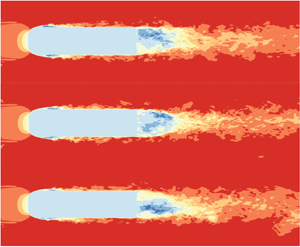
It is possible to describe the large-scale dynamics with a relatively low number of modes as evidenced by figure 3 which shows three instantaneous fields at the beginning figure 3($a$), in the middle figure 3($b$) and at the end figure 3($c$) of the first switch. Each time stamp of the switch is defined as $a_1^v$ maximum, zero and minimum. The times are represented by red vertical lines in the shaded area of figure 4. The full fields (figure 3a,b,c) can be compared with their reconstructions (figure 3d,e,f) based on the mean (figure 1) and the six most energetic POD modes (figure 2a,b). The time evolution of the first two fluctuating amplitudes $a_1^v$ and $a_2^v$ are represented in figure 4. We can see that the coefficient of the switch mode $a_2^v$ is maximum during the switch. In the next section, we examine if the large-scale signature of the switch can be reproduced with a low-dimensional model.

Figure 3. Velocity in a horizontal mid-plane at (a,d) the beginning, (b,e) during when $a_1^{v}=0$ and (c,f) at the end of the switch; (a–c) instantaneous field; (d–f) reconstructed field using the mean and the six first fluctuating modes.

Figure 4. Amplitudes of the POD velocity modes ($a$) $a_1^v$ and ($b$) $a_2^v$. The vertical lines in the shaded area corresponding to the switch represent the times of figure 3.

4. Low-dimensional model

4.1. Derivation

We give a brief review of the derivation process (see also Podvin et al. Reference Podvin, Pellerin, Fraigneau, Evrard and Cadot2020; Soucasse et al. Reference Soucasse, Podvin, Rivière and Soufiani2020). The Navier–Stokes equations are projected onto the basis of the spatial velocity modes $\underline {\phi }_k$ for a given truncation $k \in [1, \ldots , N_T]$ and a model, or system of $N_T$ ordinary differential equations (ODEs) is obtained. The model is of the form

(4.1)\begin{equation} \dot{a}_k^v= L_{km} a_m^v + Q_{kmp} a_m^v a_p^v + T_{k}. \end{equation}

The linear term $L_{km}$ is due to the viscous dissipation $L_{km}= \int \nu \Delta \underline {\phi }_{m} \boldsymbol {\cdot } \underline {\phi }_{k} \,\textrm {d}\kern0.06em \underline {x}$ and is found to be essentially diagonal. The quadratic terms $Q_{kmp}$ can be written in symmetric form as

(4.2)\begin{equation} Q_{kmp}= \tfrac{1}{2}(2-\delta_{mp}) \int (\underline{\phi}_p \boldsymbol{\cdot} \boldsymbol{\nabla} \underline{\phi}_{m}) + \underline{\phi}_m \boldsymbol{\cdot} \boldsymbol{\nabla} \underline{\phi}_p) \boldsymbol{\cdot} \underline{\phi}_{k} \,\textrm{d}\kern0.7pt \underline{x}. \end{equation}

They represent the nonlinear interaction of the resolved modes, including the mean field corresponding to mode 0. Here $T_k$ is a closure term representing the contribution of the unresolved stresses (associated with the modes excluded from the truncation) to the evolution of the amplitude $a_k$. As has been shown in Podvin & Sergent (Reference Podvin and Sergent2017), the closure term can be modelled as $T_k = -\alpha _k\sum _{p=1}^{N_T} (\lambda _p + |a_p^v|^2 ) a_k^v + \epsilon _k$, where $\lambda _p$ is the energy of mode p and $\epsilon _k$ is a noise-like perturbation. The value of $\alpha _k$ is determined by requiring that for some equilibrium state $a_p^{v,eq}$ inferred from the direct numerical simulation (DNS), the total contribution $A_k= L_{kk} a_k^{v} + Q_{kk0} a_k^v + T_k$ cancels when $a_k^v=a_k^{v,eq}$ for $k=1, \ldots , 6$, and $\epsilon _k=0$, which yields

(4.3)\begin{equation} \alpha_k=\frac{L_{kk}+Q_{kk0}}{\sum\limits_{p = 1}^{N_T} (\lambda_p + |a_p^{v,eq}|^2)}, \end{equation}

which yields

(4.4)\begin{equation} A_k=\alpha_k a_k^v \sum_{p = 1}^{N_T}(|a_p^{v,eq}|^2- |a_p^v|^2). \end{equation}

Since (4.4) is derived from relatively crude modelling assumptions, some adjustment in the definition of $A_k$ may be needed in the model.

4.2. Seven-mode truncation

In what follows, we consider a seven-mode truncation for the full field $(N_T=6)$. Since the amplitude of the mean field is constant, i.e. $a_0=1$, the model is six-dimensional. The model includes the deviation mode, the switch mode and the von Kármán shedding modes. We note that the model is different from that of Podvin et al. (Reference Podvin, Pellerin, Fraigneau, Evrard and Cadot2020) which did not include the switch mode $a_2$. If only the deviation mode is retained in the model, the system is formally analogous to the model of Rigas et al. (Reference Rigas, Morgans, Brackston and Morrison2015). The quadratic interactions coefficients were thresholded: values smaller than $5 \times 10^{-3}$ were not included in the model. It remains to determine the small-scale modelling parameters $\alpha _k$ and $\epsilon _k$. The noise level r.m.s. $\sigma _k=\langle \epsilon _k^2\rangle ^{1/2}$ was chosen to be equal to a constant value $\sigma$ for all modes and was estimated to be of the order of $\sigma \sim \alpha _k \sum _{p \geqslant 1}^{N_T} \lambda _p \sim 0.1$. In order to determine $\alpha _k$, we use (4.3). The equilibrium state was defined as $a_1^{eq}=\pm 1$, $a_2^{eq}=0$ (no switch mode), $|a_{2i-1}^{eq}|^2+|a_{2i}^{eq}|^2=2$ for $i=2, 3$ (constant vortex shedding intensity). Given the eigenvalues $\lambda _2=0.057$, $\lambda _3=0.015$ and $\lambda _i \sim 0.01$ for $i=3, \ldots , 6$, (4.3) yields values of $\alpha _k$ in the range $[0.85, 1.25]$. Since the small-scales modelling is relatively crude, we used a single value $\alpha _k= \alpha = 1$ for all modes. The system can then be written in normalized form as

(4.5)$$\begin{gather} \dot{a}_0 = 0, \end{gather}$$

(4.6)$$\begin{gather}\dot{a}_1 = A_1 + 0.011 a_1 a_2 + 0.019 a_0 a_3 + 0.023 a_0 a_4 + 0.045 a_3 a_5 + 0.005 a_1 a_6 + \epsilon_1, \end{gather}$$

(4.7)$$\begin{gather}\dot{a}_2 = A_2+ 0.12 a_0 a_5 + 0.11 a_0 a_6 + 0.007 a_2 a_3 -0.018 a_1^2 + 0.018 a_0^2 + \epsilon_2, \end{gather}$$

(4.8)$$\begin{gather}\dot{a}_3 = A_3 + 1.08 a_0 a_4 - 0.02 a_0 a_1 +0.037 a_1 a_6 -0.025 a_2 a_4 + \epsilon_3, \end{gather}$$

(4.9)$$\begin{gather}\dot{a}_4 = A_4 - 1.08 a_0 a_3 - 0.16 a_0 a_1 -0.04 a_1 a_5 +0.025 a_2 a_3 + \epsilon_4, \end{gather}$$

(4.10)$$\begin{gather}\dot{a}_5 = A_5 + 1.18 a_0 a_6 - 0.13 a_0 a_2 +0.035 a_2 a_3 -0.013 a_1 a_3 + 0.029 a_1 a_4 -0.013a_2^2 + \epsilon_5, \end{gather}$$

(4.11)$$\begin{gather}\dot{a}_6 = A_6 - 1.18 a_0 a_5 - 0.26 a_0 a_2 -0.026 a_2 a_5 -0.02 a_1 a_3 + \epsilon_6, \end{gather}$$

where the numerical quadratic coefficients $\tilde {Q}_{kmp}$ are equal to $({\sqrt {\lambda _m \lambda _p}}/{\lambda _k} )Q_{kmp}$, and $A_k$ is based on the following non-dimensional adaptation of (4.4) to account for the energy transfer to the unresolved scales:

(4.12)\begin{equation} A_k= \alpha_k a_k \sum_{p = 1}^{N_T}(\beta_k |a_p^{v,eq}|^2- |a_p^v|^2) = \alpha a_k \sum_{p=1}^{6}\lambda_p (\beta_k |a_p^{eq}|^2- |a_p|^2), \end{equation}

where $\beta _k = 1$ for $k \leqslant 2$ and $\beta _k=0.8$ for $k \geqslant 3$. The mode $a_0$ corresponding to the mean velocity is equal to 1. We point out that the evolution of a mode of a given symmetry is governed by interactions of modes obeying the same symmetry. The deviation mode is therefore controlled by its interaction with the switch mode, but also by cross-interactions between vortex-shedding modes of opposite symmetries.

4.3. Results

The model was integrated over 20 000 convective time units with and without noise. We first consider the integration without noise ($\sigma =0$). The time series are represented in figure 5(a) and can be compared with the normalized amplitudes obtained from the simulation in figure 4. We can see that the model displays chaotic dynamics characterized by switches. The inter-switch time is random and of the order of a few thousand units, in agreement with Grandemange et al. (Reference Grandemange, Gohlke and Cadot2013). The duration of the switch itself is $O(100)$ convective units, in good agreement with the simulation. The intensity of the vortex shedding increases drastically during the switches (figure 5a, bottom two rows). This suggests that the shedding modes symmetrize the wake. At the onset of the switch, $a_2$ increases then decreases sharply. It becomes strongly positive and reaches its maximum when $a_1$ goes through zero, in agreement with the DNS (figure 4). The model therefore does not only display spontaneous switches, but also captures the specific dynamics of the switch mode $a_2$. We then consider the integration of the model with noise. Figure 5(b) shows the evolution of the amplitudes for a model with a noise r.m.s. of $\sigma = 0.07$. As expected, the inter-switch time interval decreased with an increasing noise level but remained of the order of $10^3$ units for $\sigma \in [0.05, 0.1]$. As can be seen in figure 5(b), the noise may trigger a switch without any shedding intensity increase as shown for the first switch example (see caption). However, the second switch example is clearly associated with an $a_5$ increase corresponding to the shedding in the vertical direction.

Figure 5. Amplitudes of POD modes 1, 2, 3 and 5 integrated in the model ($a$) without and ($b$) with noise. Vertical dashed lines locate time at which $a_1=0$ for two switching examples.

The addition of noise leads to time evolutions which are closer to the DNS amplitudes, as can also be seen in figure 6, which compares the phase portraits in the $(a_1, a_2)$ space for the model without noise, the model with noise and the DNS. We note that when noise is added to the model, $a_2$ can take negative values between switches, which is more consistent with DNS observations (there is still a discrepancy, which is due to the choice of the particular equilibrium $a_2^{eq}=0$). This is confirmed by comparison of the spectra shown in figure 7. The characteristic frequencies associated with vortex shedding are clearly identified in the model without noise, while an excellent agreement in both the dominant frequencies and in the general shape and levels of the spectra is observed between the model with noise and the DNS. The model therefore captures the main time scales of the dynamics, including those of the switch.

Figure 6. Phase portraits in the $(a_1, a_2)$ space: (a) in model without noise; (b) in model with noise level $\sigma =0.07$; (c) in DNS.

Figure 7. Comparison of the spectra of the velocity mode amplitudes $a_k$ in the DNS and in the model without and with a noise level $\sigma$.

Further insight into the physics of the model can be obtained by artificially manipulating the energy levels of the modes. The results of these numerical experiments are presented in figure 8. Excluding the switch mode from the model (see figure 8a) i.e. setting $a_2=0$ suppresses switches in the absence of noise – the system remains near one of the equilibrium states – and strongly limits them in the presence of noise which was obtained with the same noise perturbation as in figure 5(b). This is confirmed by linear stability of the quasi-steady state, according to which the equilibrium is stable if the switch mode is omitted from the model. The influence of the vortex-shedding intensity can be examined by modifying the eigenvalues $\lambda _i \rightarrow s \lambda _i$ for $i=3, \ldots , 6$. This leads to modifications in the quadratic terms $\tilde {Q}_{kmp}$ as well as in $A_k$, with a new equilibrium state $|a_{2i-1}^{eq}|^2+|a_{2i}^{eq}|^2=2s$ for $i=2, 3$ and a new value of $\alpha$ in order to satisfy (4.3), (4.4). Integration of the model without noise is presented in figure 8(b) for $s=1.5$ and $s=0.5$. Spontaneous switching is more frequent when the energy is increased by 50 % ($s=1.5$), as can be seen from comparison with figure 5, and is suppressed when the vortex-shedding energy is reduced to 50 % ($s=0.5$) of its expected value. This suggests that both the switch and vortex-shedding modes are key players in the switching process. We speculate that the vortex-shedding modes could be considered as a periodic forcing that introduces chaotic behaviour at longer time scales in the 2-D system constituted by the deviation and the switch modes, in a manner that could be reminiscent of forced nonlinear oscillators such as the Duffing or the Van der Pol equation (Guckenheimer & Holmes Reference Guckenheimer and Holmes1983).

Figure 8. Amplitudes of POD modes 1 and 3 in modified models: (a) models with no switch mode $a_2=0$ with (solid line) and without noise (dotted line), (b) models with no noise and modified vortex shedding energy $s\lambda _i$, $i=3,\ldots 6$ (see text) for $s=1.5$ (solid line) and $s=0.5$ (dotted line).