


1. Introduction
The instability of liquid jets and cylindrical columns of ideal fluids has been researched rigorously for over a century. The well-known Plateau–Rayleigh instability describes the break-up of a capillary jet into droplets, for linear axisymmetric perturbations of wavelengths longer than the radius of the jet (Rayleigh Reference Rayleigh1878). It has been shown in the ferro-hydrodynamic literature that the Plateau–Rayleigh instability for a ferrofluid jet can be stabilised by a sufficiently strong azimuthal magnetic field (Bashtovoi & Krakov Reference Bashtovoi and Krakov1978; Arkhipenko et al. Reference Arkhipenko, Barkov, Bashtovoi and Krakov1980; Rannacher & Engel Reference Rannacher and Engel2006). Ferrofluids are colloidal fluids, consisting of magnetic solids such as magnetite, suspended in a carrier solution, usually water, kerosene or oils. The liquid becomes magnetised in the presence of a magnetic field, and to prevent agglomeration, the nanoparticles are either electrically charged or coated in a surfactant. An investigation into the stability of jets or columns of ferrofluid could be useful for technological, industrial and biomedical applications. In industry, they are most commonly used for dynamic sealing and heat dissipation (Scherer & Figueiredo Neto Reference Scherer and Figueiredo Neto2005), and there has been investigation into their use in inkjet printing (Charles Reference Charles1987; Abdel Fattah, Ghosh & Puri Reference Abdel Fattah, Ghosh and Puri2016) and three-dimensional printing (Löwa et al. Reference Löwa, Fabert, Gutkelch, Paysen, Kosch and Wiekhorst2019), where the jet disintegrates into drops that are then directed by a magnetic field. Moreover, there have been recent biomedical advances in their use in hyperthermia treatment (Zhang, Gu & Wang Reference Zhang, Gu and Wang2007) and magnetic drug targeting, experimentally (Asfer, Saroj & Panigrahi Reference Asfer, Saroj and Panigrahi2017) and theoretically (Voltairas, Fotiadis & Michalis Reference Voltairas, Fotiadis and Michalis2002; Gonella et al. Reference Gonella, Hanser, Vorwerk, Odenbach and Baumgarten2020).
The governing equations are discussed in § 2, and in § 3, the linear stability of a column of ferrofluid centred on a straight rigid wire, surrounded by another ferrofluid of different magnetic susceptibility, is investigated. A current runs through the wire, producing an azimuthal magnetic field, resulting in a magnetic stress at the interface of the fluids. The critical parameter is the magnetic Bond number, which measures the ratio between the capillary pressure and magnetic forcing from the current through the wire. The linear stability of a ferrofluid jet has been studied in the literature but with limiting assumptions. Arkhipenko et al. (Reference Arkhipenko, Barkov, Bashtovoi and Krakov1980) consider an irrotational inviscid ferrofluid jet, and show that increasing the current such that  $B>1$ produces a stable system. Of the previous works, Bashtovoi & Krakov (Reference Bashtovoi and Krakov1978) and Rannacher & Engel (Reference Rannacher and Engel2006) consider non-axisymmetric disturbances, where they assume an inviscid irrotational system, but the experimental work performed by Arkhipenko et al. (Reference Arkhipenko, Barkov, Bashtovoi and Krakov1980) and Bourdin, Barci & Falcon (Reference Bourdin, Barci and Falcon2010) suggests that viscous effects are important in the development of the instability. Cornish (Reference Cornish2018) considers the highly viscous limit, and Canu & Renoult (Reference Canu and Renoult2021) consider a Newtonian ferrofluid jet, surrounded by a Newtonian non-magnetic fluid. Both works consider axisymmetric disturbances, and the results obtained by Canu & Renoult (Reference Canu and Renoult2021) show that accounting for viscosity agrees better with the experimental results of Arkhipenko et al. (Reference Arkhipenko, Barkov, Bashtovoi and Krakov1980) and Bourdin et al. (Reference Bourdin, Barci and Falcon2010) than the inviscid system. Moreover, Canu & Renoult (Reference Canu and Renoult2021) highlight the importance of having a surrounding liquid to mirror experimental conditions and for drug targeting applications. Blyth & Parau (Reference Blyth and Parau2014) and Doak & Vanden-Broeck (Reference Doak and Vanden-Broeck2019) also consider the effect of a non-magnetic fluid surrounding the jet, but in the inviscid limit. Korovin (Reference Korovin2004) considers the surrounding liquid being a ferrofluid, filling a cuvette, rather than an infinite domain. Performing axisymmetric perturbations localised to the interface between the two fluids, the dispersion relation is derived using a modified equation of motion. He finds the thickness of the inner fluid to be of importance, and that the drops produced from the perturbation are different to when a gas is the surrounding medium. Thus we allow both fluids to be ferrofluids, and consider both axisymmetric and non-axisymmetric disturbances to the system with arbitrary Reynolds number. We give an analytical solution to the perturbed linearised Navier–Stokes equation and an implicit expression for the growth rate of the disturbance. For a given Reynolds number, a numerical root solver is used to find the growth rate for given wavenumbers, magnetic susceptibilities, strength of current and the wire radius. In the inviscid and highly viscous limits, a dispersion relation is obtained analytically, giving a stability condition.
For a non-ferrofluid jet, Christiansen (Reference Christiansen1955) found axisymmetric modes to be the most unstable (for non-axisymmetry with inertial effects), and we prove that this is true when the inner ferrofluid has a larger susceptibility than the outer. In this case, the system is linearly unstable to axisymmetric disturbances only, and  $B>1$ results in stability of all wavelengths, supporting previous works. In contrast, when the outer fluid has a larger susceptibility, axisymmetric and non-axisymmetric modes are unstable, and as the wire radius shrinks, non-axisymmetric disturbances become the most unstable at low Reynolds number. Moreover, increasing the current in the wire will not suppress all unstable modes if the outer fluid has a higher susceptibility than the inner fluid. Bashtovoi & Krakov (Reference Bashtovoi and Krakov1978) show that adding an axial field will stabilise an inviscid irrotational ferrofluid column, and we prove this for our system in both the inviscid and highly viscous regimes, irrespective of which fluid has a higher susceptibility. We show numerically that this holds for arbitrary Reynolds number too.
When a magnetic fluid is subject to a non-uniform magnetic field, the magnetic particles are attracted to the region of highest field intensity to obtain the minimum energy configuration (Scherer & Figueiredo Neto Reference Scherer and Figueiredo Neto2005). The results outlined in § 3 and the analysis performed by Zelazo & Melcher (Reference Zelazo and Melcher1969) for a two-fluid layer in a planar domain agree that when the field decreases outwards (upwards), and the stronger ferrofluid is the inner (lower) fluid, magnetic forcing is stabilising. Yet if the field decreases outwards (upwards), and the stronger ferrofluid is the outer (upper) fluid, then magnetic forcing is destabilising due to the region with largest magnetic susceptibility not being located where the field is strongest. This motivates the investigation of the stability of one ferrofluid, whose susceptibility varies continuously with radius, centred on a current-carrying wire, with an associated field decreasing as the reciprocal of the radius. In § 4, we prove that the stability of the system is determined by the sign of the gradient of the susceptibility with respect to the field strength, and prove that adding an axial field can suppress the instability.
Some works have used nonlinear theory to analyse the behaviour of a ferrofluid jet. Blyth & Parau (Reference Blyth and Parau2014) use a fully nonlinear numerical model to show that axisymmetric solitary waves propagate at the surface of an inviscid column of ferrofluid, and compare their results with the experimental work by Bourdin et al. (Reference Bourdin, Barci and Falcon2010), who show the existence of axisymmetric periodic and solitary waves at the interface of a ferrofluid jet in a cylindrical domain. Doak & Vanden-Broeck (Reference Doak and Vanden-Broeck2019), as well as studying the linear stability, use a numerical model to find stable travelling wave solutions on a ferrofluid jet. Cornish (Reference Cornish2018) uses weakly nonlinear stability theory and long wave theory for both a highly viscous and an inviscid axisymmetric jet, studying the resultant drop formation. In this paper, we focus solely on linear stability analysis.
There is a direct analogue between a ferrofluid subject to a magnetic field in ferro-hydrodynamics and a dielectric exposed to a gradient electric field in electro-hydrodynamics (Zelazo & Melcher Reference Zelazo and Melcher1969; Rosensweig Reference Rosensweig1985). Nayyar & Murty (Reference Nayyar and Murty1960) and Garcia et al. (Reference Garcia, Gonzz, Ramos and Castellanos1997) study, respectively, the stability of inviscid and viscous dielectric liquid columns, subject to a longitudinal electric field. Nayyar & Murty (Reference Nayyar and Murty1960) use an energy argument to show that the electric field has a stabilising effect. Garcia et al. (Reference Garcia, Gonzz, Ramos and Castellanos1997) consider axisymmetric perturbations to the system and produce a dispersion relation, showing that viscous dissipation and dielectric forces at the interface work to stabilise the system. A crucial difference between the dielectric work on jets and the problem in this paper is the presence of a wire and the associated azimuthal field.
2. Magnetic force and stress tensor
We assume that the magnetisation  $\boldsymbol {M}$ is collinear with the magnetic field
  $\boldsymbol {H}$ such that
  $\boldsymbol {M}=\chi \boldsymbol {H}$, where
  $\chi$ is the magnetic susceptibility. The field satisfies
 \begin{equation} \boldsymbol{\nabla}\times\boldsymbol{H}=0, \end{equation}
and the induced field  $\boldsymbol {B}$ satisfies
 \begin{equation} \boldsymbol{\nabla}\boldsymbol{\cdot} \boldsymbol{B}=0. \end{equation}
Equation (2.1) allows us to define a magnetic potential  $\phi$ such that
 \begin{equation} \boldsymbol{H}=\boldsymbol{\nabla}\phi. \end{equation}
Due to collinearity,  $\boldsymbol {B}=\mu _0(1+\chi )\boldsymbol {H}$, where
  $\mu _0$ is the magnetic permeability of the fluid, and therefore
 \begin{equation} \boldsymbol{\nabla} \boldsymbol{\cdot}((1+\chi)\,\boldsymbol{\nabla}\phi)=0. \end{equation}
At an interface, we require continuity of the normal component of  $\boldsymbol {B}$,
 \begin{equation} \left[\mu_0(1+\chi)\,\boldsymbol{\nabla}\phi\boldsymbol{\cdot}\boldsymbol{n}\right]=0, \end{equation}
and continuity of the tangential component of  $\boldsymbol {H}$,
 \begin{equation} \left[\boldsymbol{\nabla}\phi\boldsymbol{\cdot}\boldsymbol{\tau}\right]=0, \end{equation}
where  $\boldsymbol {n}$ and
  $\boldsymbol {\tau }$ are respectively the unitary normal and tangential vectors to the interface, and the square brackets denote the jump across it.
Rosensweig (Reference Rosensweig1985) gives the stress tensor for a Newtonian isothermal ferrofluid as
 \begin{equation} \boldsymbol{\mathsf{T}}={-}\mu_0\left(\int_0^H\chi H \,{\rm d}H+\tfrac{1}{2}H^2\right)\boldsymbol{\mathsf{I}}-p\boldsymbol{\mathsf{I}} +\boldsymbol{BH}^{\rm T}+\eta(\boldsymbol{\nabla}\boldsymbol{u} +(\boldsymbol{\nabla}\boldsymbol{u})^{\boldsymbol{T}}), \end{equation}
where  $H=|\boldsymbol {H}|$,
  $\eta$ is the viscosity,
  $p$ is the pressure,
  $\boldsymbol {u}$ is the velocity of the fluid, and strictive effects have been neglected on account of there being no physiochemical phase change in the flow. The force density due to magnetic effects, for a ferrofluid subject to
  $\boldsymbol {H}$, is
 \begin{equation} \boldsymbol{f}={-}\boldsymbol{\nabla}\left(\mu_0\int_0^H(1+\chi)H\,{\rm d}H\right) +\mu_0(1+\chi)H\,\boldsymbol{\nabla}H, \end{equation}
and if  $\chi$ is independent of
  $\boldsymbol {H}$, then
 \begin{equation} \boldsymbol{f}={-}\frac{\mu_0H^2}{2}\,\boldsymbol{\nabla}\chi. \end{equation}
Now,  $\boldsymbol {f}$ appears in the Navier–Stokes equation as
 \begin{equation} \rho\,\frac{{\rm D}\boldsymbol{u}}{{\rm D}t}+\boldsymbol{\nabla}p=\eta\,{\nabla}^2\boldsymbol{u}+\boldsymbol{f}, \end{equation}
where  $\rho$ is the density of the fluid. Taking the curl of (2.10) gives
 \begin{equation} \rho\,\frac{{\rm D}\boldsymbol{\omega}}{{\rm D}t}=\eta((\boldsymbol{\omega}\boldsymbol{\cdot} \boldsymbol{\nabla})\boldsymbol{u}+{\nabla}^2\boldsymbol{\omega})+\mu_0H\,\boldsymbol{\nabla}\chi\times\boldsymbol{\nabla}H, \end{equation}
where  $\boldsymbol {{\omega }}=\boldsymbol {\nabla }\times \boldsymbol {{u}}$. Equation (2.11) holds for both (2.8) and (2.9), and it follows that if
  $H=H(\chi )$, then we have a stationary state.
3. Two-fluid system
3.1. Formulation of the problem
We consider a column of ferrofluid, fluid 1, with magnetic susceptibility  $\chi =\chi _1$, centred on a rigid wire with radius
  $a$. We choose the cylindrical system
  $(r,\theta,z)$ such that
  $r$ and
  $\theta$ are the radial and azimuthal coordinates, and
  $z$ points along the wire. In the stationary state, fluid 1 is in the region
  $a< r< R$ and is surrounded by another ferrofluid, fluid 2, whose domain is unbounded, with susceptibility
  $\chi =\chi _2$. Both fluids are incompressible and isothermal, with constant density
  $\rho$, viscosity
  $\eta$, and permeability
  $\mu _0$. A steady electric current
  ${\boldsymbol {J}}=J_0{\boldsymbol {e}_z}$ runs through the wire, producing an azimuthal magnetic field
  ${\boldsymbol {H}}=J_0/2{\rm \pi} r\boldsymbol {e}_{\theta }$, where
  $\boldsymbol {e}_z$ is the unit vector in the
  $z$ direction, and
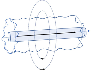
  $\boldsymbol {e}_{\theta }$ is the unit vector in the anticlockwise, azimuthal direction. The set-up is shown in figure 1.

Figure 1. Schematic of the two-fluid system.
Take  $R$ as the length scale, and define
  $a=a_*R$. We non-dimensionalise pressure as
  $p=\sigma p_*/R$, where
  $\sigma$ is the surface tension, and non-dimensionalise the field as
  $\boldsymbol {H}=J_0\boldsymbol {H_*}/2{\rm \pi} R$, and pick the time scale,
  $T$, to be
  $T=\eta R/\sigma$, such that the velocity is non-dimensionalised as
  $\boldsymbol {u}=\sigma /\eta \boldsymbol {u}_*$. The starred variables are dimensionless, but we drop the stars from here on. Equation (2.10) becomes
 \begin{equation} {{Re}}\,\frac{{\rm D}\boldsymbol{u}}{{\rm D}t}+\boldsymbol{\nabla}p={\nabla}^2\boldsymbol{u}+B\boldsymbol{f}, \end{equation}
where
 \begin{equation} {{Re}}=\frac{\rho \sigma R}{\eta^2} \end{equation}
is the Reynolds number, and
 \begin{equation} B=\frac{\mu_0J_0^2}{4{\rm \pi}^2 R\sigma} \end{equation}
is the magnetic Bond number. Since
 \begin{equation} \left. \begin{array}{ll@{}} \displaystyle \chi=0, & {\rm for}\ r \leq a,\\ \displaystyle \chi=\chi_1, & {\rm for}\ a< r < R,\\ \displaystyle \chi=\chi_2, & {\rm for}\ r \geq R, \end{array}\right\} \end{equation}
 $\chi$ is always constant, resulting in
  $\boldsymbol {f}=\boldsymbol {0}$ in (3.1), and magnetic effects are felt only at the interface.
Initially, both fluids are at rest and the interface between the two fluids is located at  $r=1$. We consider perturbations to the surface such that the surface is located at
 \begin{equation} r=1+\epsilon\,{\rm Re}(\hat{S}\zeta), \end{equation}
where  $\zeta =\exp \left ({\textrm {i}(kz+m\theta )+st}\right )$,
  $\epsilon \ll 1$,
  $k,m$ are real and positive wavenumbers,
  $\hat {S}$ may be a complex constant (or it could be unity), and
  $s$ is the growth rate of the disturbance and could be complex. In (3.5), the real part of the perturbation is taken, and this is done from here on for the other variables, but it is not written explicitly. The normal vector to the surface becomes
 \begin{equation} \boldsymbol{{n}}=\left(1,-\frac{\epsilon{\rm i}m\hat{S}\zeta}{r},-\epsilon{\rm i}k\hat{S}\zeta\right)^{\rm T}, \end{equation}
and the tangential vectors are
 \begin{equation} {\boldsymbol{{\tau}_1}}=(\epsilon{\rm i}k\hat{S}\zeta,0,1)^{\rm T}, \quad \boldsymbol{{\tau}_2}=\left(\frac{\epsilon{\rm i}m\hat{S}\zeta}{r},1,0\right)^{\rm T}. \end{equation}
The perturbed pressure  $p^{(i)}$ and velocity
  $\boldsymbol {u}^{(i)}$, where
  $i=1,2$ for fluids
  $1$ and
  $2$, are
 \begin{equation} p^{(i)}=p_0+\epsilon\,\hat{p}^{(i)}(r)\,\zeta \quad {\rm and} \quad \boldsymbol{u}^{(i)}=\epsilon\,\hat{\boldsymbol{u}}^{(i)}(r)\,\zeta, \end{equation}
where  $p_0$ is constant. The perturbations satisfy
 \begin{equation} \boldsymbol{\nabla}\boldsymbol{\cdot} \hat{\boldsymbol{u}}=0 \quad {\rm and} \quad s\,{{Re}}\,\hat{\boldsymbol{u}}+\boldsymbol{\nabla}\hat{p}={\nabla}^2\hat{\boldsymbol{u}}. \end{equation}
In component form we have
 \begin{gather} (r\hat{u})'+{\rm i}m\hat{v}+{\rm i}kr\hat{w}=0, \end{gather}
 \begin{gather} r^2\hat{p}'={-}2{\rm i}m\hat{v}-\hat{u}+r^2\hat{u}''+r\hat{u}'-(m^2+\bar{k}^2r^2)\hat{u}, \end{gather}
 \begin{gather} {\rm i}mr\hat{p}={-}\hat{v}+2{\rm i}m\hat{u}+r^2\hat{v}''+r\hat{v}'-(m^2+\bar{k}^2r^2)\hat{v}, \end{gather}
 \begin{gather} {\rm i}kr^2\hat{p}=r^2\hat{w''}+rw'-(m^2+\bar{k}^2r^2)\hat{w}, \end{gather}
where  $'$ denotes the first derivative with respect to
  $r$, and
  $\bar {k}=\sqrt {k^2+s\,{{Re}}}$. The general solution is in terms of the modified Bessel functions of the first and second kind,
  $\textrm {I}_n(z)$ and
  $\textrm {K}_n(z)$, respectively, where we write
  $\textrm {I}_n, \textrm {K}_n$ when
  $z=kr$, and
  $\bar {\textrm {I}}_n, \bar {\textrm {K}}_n$ when
  $z=\bar {k}r$, but give the argument otherwise. The general solution of (3.9a,b) is modified from Saville (Reference Saville1971) and Mestel (Reference Mestel1996) to account for the inner wire at
  $r=a$, and is found to be
 \begin{align} \hat{p}^{(i)} & = c_1^{(i)}{\rm I}_m + c_2^{(i)}{\rm K}_{m}, \end{align}
 \begin{align} \hat{u}^{(i)} & ={-}\frac {1}{(s\,{{Re}})^{2}r} \left(c_1^{(i)}(kr{\rm I}_{m+1}+m{\rm I}_m)+c_2^{(i)}(m{\rm K}_m-kr{\rm K}_{m+1})\right)\nonumber\\ &\quad -\frac{{\rm i}k}{\bar{k}}\left(c_3^{(i)}\bar{{\rm I}}_{m+1}+c_4^{(i)}\bar{{\rm K}}_{m+1}\right)+\frac{2m}{\bar{k}r}\left(c_5^{(i)}\bar{{\rm I}}_m+c_6^{(i)}\bar{{\rm K}}_{m}\right),\end{align}
 \begin{align} \hat{v}^{(i)}& = \left( {{\frac {-c_3^{(i)}k}{\bar{k}}}}+2{\rm i}c_5^{(i)} \right) \bar{{\rm I}}_{m+1}+{\frac {2{\rm i}m}{\bar{k}r}}\left(c_5^{(i)}\bar{{\rm I}}_m+c_6^{(i)}\bar{{\rm K}}_{m}\right)-\left({{\frac {c_4^{(i)}k}{\bar{k}}}}+2{\rm i}c_6^{(i)} \right) \bar{{\rm K}}_{m+1}\nonumber\\ &\quad -\frac{{\rm i}m}{{(s\,{{Re}})}^{2}r}\left(c_2^{(i)}{\rm K}_{m}+c_1^{(i)}{\rm I}_m\right),\end{align}
 \begin{align} \hat{w}^{(i)}& = {\frac {-{\rm i}k}{{(s\,{{Re}})}^{2}}}\left(c_1^{(i)}{\rm I}_m+c_2^{(i)}{\rm K}_{m}\right)+c_3^{(i)}\bar{{\rm I}}_m-c_4^{(i)}\bar{{\rm K}}_{m}, \end{align}
for constants  $c_1^{(i)},\ldots, c_6^{(i)}$. To satisfy
  $u^{(2)} \rightarrow 0$ as
  $r \rightarrow \infty$,
  $\mathrm {Re}(\bar {k})>0$ and
  $c_1^{(2)}=c_3^{(2)}=c_5^{(2)}=0$.
We perturb the magnetic potential such that
 \begin{equation} \phi^{(l)}=\theta+\epsilon\,\hat{\phi}^{(l)}(r)\,\zeta, \end{equation}
where  $l=0,1,2$ for the wire, inner fluid and outer fluid, respectively. Equation (2.4) gives
 \begin{equation} r^2\hat{\phi''}^{(l)}+\hat{\phi'}^{(l)}-(m^2+k^2r^2)\hat{\phi}^{(l)}=0, \end{equation}
with general solution
 \begin{equation} \hat{\phi}(r)^{(l)}=q_1^{(l)}{\rm I}_m+q_2^{(l)}{\rm K}_m, \end{equation}
for constants  $q_1^{(l)},q_2^{(l)}$. For
  $\hat {\phi }^{(0)}$ regular at
  $r=0$,
 \begin{equation} \hat{\phi}^{(0)}=q_1^{(0)}{\rm I}_m, \end{equation}
and imposing  $\phi ^{(2)}\rightarrow 0$, as
  $r\rightarrow \infty$ gives
 \begin{equation} \hat{\phi}^{(2)}=q_2^{(2)}{\rm K}_m. \end{equation}
Equations (2.5) and (2.6) give
 \begin{equation} (1+\chi_2)\hat{\phi}'^{(2)}-(1+\chi_1)\hat{\phi}'^{(1)}+im(\chi_1-\chi_2)\hat{S}=0 , \quad \hat{\phi}^{(1)}=\hat{\phi}^{(2)} \end{equation}
at  $r=1$, and
 \begin{equation} (1+\chi_1)\hat{\phi}'^{(1)}-\hat{\phi}'^{(0)}=0, \quad \hat{\phi}^{(1)}=\hat{\phi}^{(0)} \end{equation}
at  $r=a$, determining the constants
  $q_1^{(0)},q_1^{(1)},q_2^{(1)},q_2^{(2)}$ given in (A1)–(A4) in Appendix A.
At  $r=a$,
 \begin{equation} \hat{\boldsymbol{u}}^{(1)}=0, \end{equation}
and at  $r=1$,
 \begin{equation} \hat{\boldsymbol{u}}^{(1)}=\hat{\boldsymbol{u}}^{(2)}. \end{equation}
At the interface of the fluids, there is a normal stress condition
 \begin{equation}
[\boldsymbol{n}\boldsymbol{\cdot}\boldsymbol{T}\boldsymbol{\cdot}
\boldsymbol{n}]=\sigma\,
\boldsymbol{\nabla}\boldsymbol{\cdot} \boldsymbol{n},
\end{equation}
\begin{equation}
[\boldsymbol{n}\boldsymbol{\cdot}\boldsymbol{T}\boldsymbol{\cdot}
\boldsymbol{n}]=\sigma\,
\boldsymbol{\nabla}\boldsymbol{\cdot} \boldsymbol{n},
\end{equation}
and two tangential stress conditions
 \begin{gather} {[}\boldsymbol{n}\boldsymbol{\cdot}\boldsymbol{T}\boldsymbol{\cdot} \boldsymbol{\tau_1}]=0, \end{gather}
 \begin{gather} {[}\boldsymbol{n}\boldsymbol{\cdot}\boldsymbol{T}\boldsymbol{\cdot} \boldsymbol{\tau_2}]=0. \end{gather}
Non-dimensionalising (3.24), substituting the perturbed variables, linearising, and invoking continuity of the normal component of  $\boldsymbol {B}$, we obtain
 \begin{align}
(m^2+k^2-1+B(\chi_1-\chi_2))\hat{S}={\rm i}mB(\chi_1\hat{\phi}^{(1)}
-\chi_2\hat{\phi}^{(2)})+\hat{p}^{(1)}-
\hat{p}^{(2)}-2\hat{u}'^{(1)}+2\hat{u}'^{(2)}
\end{align}
\begin{align}
(m^2+k^2-1+B(\chi_1-\chi_2))\hat{S}={\rm i}mB(\chi_1\hat{\phi}^{(1)}
-\chi_2\hat{\phi}^{(2)})+\hat{p}^{(1)}-
\hat{p}^{(2)}-2\hat{u}'^{(1)}+2\hat{u}'^{(2)}
\end{align}
at  $r=1$. Similarly, (3.25) and (3.26) give
 \begin{equation} \hat{v}'^{(1)}-\hat{v}'^{(2)}=0 \end{equation}
and
 \begin{equation} \hat{w}'^{(1)}-\hat{w}'^{(2)}=0 \end{equation}
at  $r=1$. Equations (3.22), (3.23) (3.27)–(3.29) determine the constants
  $c_1^{(i)},\ldots, c_6^{(i)}$ given in (A13)–(A21).
The growth rate appears in the kinematic condition at  $r=1$:
 \begin{equation} s\hat{S}-\hat{u}^{(i)}=0. \end{equation}
Consequently, substituting  $\hat {u}^{(i)}$ into (3.30), we obtain
 \begin{equation}
s={-}gf(f_1(k^2+m^2-1+{B}(\chi_1-\chi_2))+f_2{B}(\chi_1-\chi_2)^2m^2),
\end{equation}
\begin{equation}
s={-}gf(f_1(k^2+m^2-1+{B}(\chi_1-\chi_2))+f_2{B}(\chi_1-\chi_2)^2m^2),
\end{equation}
where  $g, f_1, f_2>0$. Here,
  $g, f_1, f_2$ are functions of
  $m,k,a,\chi _1,\chi _2$, and
  $f$ is a function of
  $\bar {k}, m, k, a,\chi _1,\chi _2$, all given in (A10)–(A12). Since
  $\bar {k}$ is a function of
  $s$,
$s$,  $f$ is a function of
  $s$, and therefore (3.31) is an implicit relation that must be solved numerically.
3.2. Highly viscous and inviscid limits
In the limit  ${{Re}} \rightarrow 0$,
  $f\rightarrow f_v$, where
  $f_v>0$ and
  $f_v$ is no longer a function of
  $s$, given in (A22). The growth rate in the highly viscous regime,
  $s_v$, is expressed explicitly as
 \begin{equation} s_v={-}gf_v(f_1(k^2+m^2-1+{B}(\chi_1-\chi_2))+f_2{B}(\chi_1-\chi_2)^2m^2). \end{equation}
 In the inviscid limit,  $\eta \rightarrow 0$, and a more appropriate scaling for time,
  $T_I$, is
  $T_I=\sqrt {R^3\rho /\sigma }$. Since
  $T_I=\sqrt {{{Re}}}\,T$, we substitute
  $s=s_I/\sqrt {{{Re}}}$ into (3.31), where
  $s_I$ is the inviscid growth rate. Taking the limit as
  ${{Re}} \rightarrow \infty$ gives
  $f\rightarrow f_I/s_I$, where
  $f_I>0$ and
  $f_I$ is no longer a function of
  $s$, given in (A23). Consequently,
 \begin{equation} s_I^2={-}gf_I(f_1(k^2+m^2-1+{B}(\chi_1-\chi_2))+f_2{B}(\chi_1-\chi_2)^2m^2). \end{equation}
More simply, (3.33) can be obtained by taking the limit  $\eta \rightarrow 0$ in the governing equations from the outset, and applying the boundary conditions for an inviscid system (
 $\eta =0$), namely
  $\hat {u}^{(1)}=0$ at the wire, and
  $\hat {u}^{(1)}=\hat {u}^{(2)}$, (3.27), (3.29) at the interface.
Since  $f_I,f_v>0$, the system is stable (or neutrally stable), in both the inviscid and highly viscous regimes, if and only if
 \begin{equation} f_1(k^2+m^2-1+{B}(\chi_1-\chi_2))+f_2{B}(\chi_1-\chi_2)^2m^2\geq 0. \end{equation}
Note that in the inviscid regime, if (3.34) holds, then the system is neutrally stable as the growth rate is imaginary. If the inner fluid has a higher susceptibility than the outer fluid, then the system can be unstable only as a result of capillary forces. Only axisymmetric modes can be unstable when  $k<1$, and increasing the current in the wire will stabilise the system provided that
  $B(\chi _1-\chi _2)>1$. Figures 2 and 3 show the growth rate of the modes being dampened as the current in the wire is increased for the viscous and inviscid regimes, respectively.

Figure 2. Viscous growth rate,  $a=0.1$,
  $\chi _1=5$,
  $\chi _2=1$: (a)
  $B=0$, (b)
  $B=0.1$, (c)
  $B=0.25$, (d)
  $B=4$.

Figure 3. Inviscid growth rate,  $a=0.1$,
  $\chi _1=5$,
  $\chi _2=1$: (a)
  $B=0$, (b)
  $B=0.1$, (c)
  $B=0.25$, (d)
  $B=4$.
On the other hand, when the outer fluid has a higher susceptibility, capillary and magnetic forces may be destabilising. Increasing the current, thereby increasing the magnetic forcing at the interface, renders non-axisymmetric modes unstable, as well as axisymmetric modes, and for sufficiently large  $B$, all modes
  $m$ can be rendered unstable. Figures 4–6 show that increasing
  $B$ results in an increase in unstable modes, and increases the magnitude of their growth rates. Moreover, in the highly viscous regime, figure 5 shows
  $m=1$,
  $k\rightarrow 0$, is the most unstable mode for
  $a=0.1$, and in fact
  $s\rightarrow \infty$ as
  $k\rightarrow 0$, whereas when
  $a=0.5$ in figure 6,
  $m=0$ remains the most unstable mode. Performing a series expansion on the viscous growth rate as
  $a,k\rightarrow 0$, we find
  $s\sim \ln (ka)$ when
  $m=1$, thus
  $s\rightarrow \infty$ in the limit, but
  $s$ converges to a constant when
  $m=0$ or
  $m>1$, a result seen in the context of electro-hydrodynamics too (Saville Reference Saville1971; Mestel Reference Mestel1996). It is important to note that when comparing the inviscid regime with the viscous regime,
  $s_I$ and
  $s_v$ are on different time scales.

Figure 4. Inviscid growth rate,  $a=0.1$,
  $\chi _1=1$,
  $\chi _2=5$: (a)
  $B=0$, (b)
  $B=1$, (c)
  $B=10$.

Figure 5. Viscous growth rate,  $a=0.1$,
  $\chi _1=1$,
  $\chi _2=5$: (a)
  $B=0$, (b)
  $B=1$, (c)
  $B=10$.

Figure 6. Viscous growth rate,  $a=0.5$,
  $\chi _1=1$,
  $\chi _2=5$: (a)
  $B=0$, (b)
  $B=1$, (c)
  $B=10$.
3.3. Arbitrary Reynolds number
A numerical root solver in the program Maple is used on (3.31) for specific values of  $k,a,m,\chi _1,\chi _2,B,{{Re}}$, to find the associated growth rate of the mode. The stability condition (3.34) appears to hold for all Reynolds numbers. Figure 7 is the growth rate plotted when
  $a=0.1$,
  $k=0.5$,
  $\chi _1=1$,
  $\chi _2=5$,
  $B=0.1$, for a range of Reynolds numbers, showing two stable branches when
  $m=1$ and an unstable branch for
  $m=0$. Given a stable mode, as
  ${{Re}} \rightarrow 0$, there are two branches, both real: one branch tends to
  $s_v$, and the other tends to
  $-\infty$, the latter a result of
  ${{Re}} \rightarrow 0$ for the chosen time scale. As
  ${{Re}}$ is increased, the two branches meet and then split, becoming complex conjugates of each other, tending towards
  $\pm s_I$, where
  $s_I$ is purely imaginary for a stable mode. Given an unstable mode, we get one branch, starting at
  $s_v$ and tending to
  $|s_I|$. There exists a branch that tends to the negative inviscid root,
  $-|s_I|$, but this is invalid for finite
  ${{Re}}$, since the boundary conditions require
  $\mathrm {Re}({\bar {k}})\geq 0$. When
  $\chi _2>\chi _1$, and
  $a,k$ are sufficiently small,
  $m=1$ is more unstable than
  $m=0$. Yet for all
  $k$,
$k$,  $m=1$ is the most unstable mode only for sufficiently small
  ${{Re}}$. This is shown in figure 8, where the growth rate is plotted against
  $k$ for different Reynolds numbers, showing that when
  ${{Re}}=0.001,0.1$,
  $m=1$ is the most unstable mode, but for the other Reynolds numbers shown, it is not. We find that increasing the current in the wire stabilises the system if
  $\chi _1>\chi _2$ for all Reynolds numbers. Figures 7 and 9, where
  $\chi _2>\chi _1$, show that increasing
  $B$ from
  $B=0.1$ to
  $B=0.5$ renders the mode
  $m=1$ unstable, and we find that for all Reynolds numbers, increasing the current does not stabilise the system if
  $\chi _2>\chi _1$, but renders more modes unstable.

Figure 7. Growth rate plotted when  $a=0.1$,
  $k=0.5$,
  $\chi _1=1$,
  $\chi _2=5$ and
  $B=0.1$ for arbitrary
  ${{Re}}$. Panels (a) and (b) plot, respectively, the real and imaginary parts of
  $s$. The
  $m=0$ branch is purely real, but the
  $m=1$ branch starts as real for low
  ${{Re}}$ and then becomes a complex conjugate pair.

Figure 8. Growth rate plotted against  $k$, for arbitrary
  ${{Re}}$, when
  $a=0.1$,
  $\chi _1=1$,
  $\chi _2=5$,
  $B=10$: (a)
  ${{Re}}=0.0001$, (b)
  ${{Re}}=0.1$, (c)
  ${{Re}}=0.5$, (d)
  ${{Re}}=1$, (e)
  ${{Re}}=10$, ( f)
  ${{Re}}=100$.

Figure 9. Growth rate plotted when  $a=0.1$,
  $k=0.5$,
  $\chi _1=1$,
  $\chi _2=5$ and
  $B=0.5$ for arbitrary
  ${{Re}}$.
3.4. Stabilisation with an axial field
To stabilise the system, irrespective of whether  $\chi _2>\chi _1$ or
  $\chi _1>\chi _2$, we consider
  $\boldsymbol {H}_0=(0,1/r,Z)^\textrm {T}$,
  $Z$ constant, thereby adding an axial field. It follows that
 \begin{equation} \phi_0=\theta +Zz, \end{equation}
and we perform analysis analogous to that in § 3.1. The general solutions (3.14), (3.17) still hold, and  $\hat {\phi }^{(0)},\hat {\phi }^{(2)}$ are still given by (3.18) and (3.19), respectively. At
  $r=a$, we apply (3.21) and (3.22). At
  $r=1$, we apply (3.23), (3.28), (3.29), but (2.5), (2.6), (3.24) now give
 \begin{equation} (1+\chi_2)\hat{\phi}'^{(2)}-(1+\chi_1)\hat{\phi}'^{(1)}+{\rm i}(m+kZ)(\chi_1-\chi_2)\hat{S}=0 , \quad \hat{\phi}^{(1)}=\hat{\phi}^{(2)}, \end{equation}
and
 \begin{align}
(m^2+k^2-1+B(\chi_1-\chi_2))\hat{S}&={\rm i}(m+kZ)B(\chi_1\hat{\phi}^{(1)}
-\chi_2\hat{\phi}^{(2)})\nonumber\\&\quad +\hat{p}^{(1)}-
\hat{p}^{(2)}-2\hat{u}'^{(1)}+2\hat{u}'^{(2)}.
\end{align}
\begin{align}
(m^2+k^2-1+B(\chi_1-\chi_2))\hat{S}&={\rm i}(m+kZ)B(\chi_1\hat{\phi}^{(1)}
-\chi_2\hat{\phi}^{(2)})\nonumber\\&\quad +\hat{p}^{(1)}-
\hat{p}^{(2)}-2\hat{u}'^{(1)}+2\hat{u}'^{(2)}.
\end{align}
We now obtain
 \begin{gather} s={-}gf(f_1(k^2+m^2-1+{B}(\chi_1-\chi_2))+f_2{B}(\chi_1-\chi_2)^2(Zk+m)^2), \end{gather}
 \begin{gather} s_v={-}gf_v(f_1(k^2+m^2-1+{B}(\chi_1-\chi_2))+f_2{B}(\chi_1-\chi_2)^2(Zk+m)^2), \end{gather}
 \begin{gather} s_I^2={-}gf_I(f_1(k^2+m^2-1+{B}(\chi_1-\chi_2))+f_2{B}(\chi_1-\chi_2)^2(Zk+m)^2), \end{gather}
analogously to (3.31), (3.32) and (3.33). Equations (3.39) and (3.40) show that a sufficiently large  $kZ$ will stabilise all modes in the inviscid and highly viscous regimes, irrespective of the sign of
  $(\chi _1-\chi _2)$, provided that
  $B\neq 0$, and this result appears to hold for all Reynolds numbers. Although extremely long waves in the
  $z$ direction,
  $k\rightarrow 0$, would remain unstable, by physical restrictions of the system,
  $k$ is bounded from zero.
4. Continuous magnetic susceptibility
Now we allow  $\chi$ to depend on position and the field. We consider one incompressible, isothermal, ferrofluid whose susceptibility varies radially. The ferrofluid is centred on the wire as shown in figure 10. Since
  $\chi$ varies with position, the magnetic forcing acts throughout the fluid. In § 3, magnetic forcing gave rise to an instability if
  $\chi _1<\chi _2$; we thus expect that
  $\textrm {d}\chi /\textrm {d}r>0$ will lead to an instability, as a result of the regions of fluid with largest
  $\chi$ being drawn to the regions of strongest field. Yet since there is no longer forcing due to surface tension at an interface, we expect
  $\textrm {d}\chi /\textrm {d}r<0$ to be stable, as both
  $\chi$ and the strength of the field decrease with the radius.

Figure 10. Schematic of the system.
Zelazo & Melcher (Reference Zelazo and Melcher1969) require the physical properties of the ferrofluid,  $\alpha _i$, to obey
 \begin{equation} \frac{{\rm D}\alpha_i}{{\rm D}t}=0, \end{equation}
but not the field dependent parts of  $\chi$. Here we assume
 \begin{equation} \frac{{\rm D}\chi}{{\rm D}t}=0, \end{equation}
so that a displaced fluid parcel retains its dependence on  $H$ and its physical properties.
Since  $\chi$ is no longer constant,
  $\boldsymbol {f}\neq 0$ in (3.1). We choose the same scaling as in § 3 to non-dimensionalise the equations. Non-dimensionalising (2.11) gives
 \begin{equation} {{Re}}\,\frac{{\rm D}\boldsymbol{\omega}}{{\rm D}t}=(\boldsymbol{\omega}\boldsymbol{\cdot} \boldsymbol{\nabla})\boldsymbol{u}+{\nabla}^2\boldsymbol{\omega}+BH\,\boldsymbol{\nabla}\chi\times\boldsymbol{\nabla}H. \end{equation}
Equation (4.3) is satisfied by  $\boldsymbol {u}=0,$
  $\chi =\chi _0(r)$,
  $H=H_0(r)$, and it follows from (3.1) that
  $p$ satisfies
 \begin{equation} \boldsymbol{\nabla}p={-}\frac{B(H_0(r))^2}{2}\,\boldsymbol{\nabla}\chi_0(r), \end{equation}
giving  $p=p_0(r)$, for a stationary state. Consider a perturbation to this stationary state such that
 \begin{equation} \chi=\chi_0(r)+\epsilon \chi_1+O(\epsilon^2), \quad \boldsymbol{H}=\boldsymbol{H}_0+\epsilon \boldsymbol{H}_1+O(\epsilon^2), \quad \boldsymbol{u}=\epsilon \boldsymbol{u_1}+O(\epsilon^2), \end{equation}
and
 \begin{equation} |\boldsymbol{H}|=H=H_0+\epsilon H_1+O(\epsilon^2),\quad {\rm where } H_0=\sqrt{\boldsymbol{H}_0\boldsymbol{\cdot}\boldsymbol{H}_0}, H_1=\frac{\boldsymbol{H}_0\boldsymbol{\cdot}\boldsymbol{H}_1}{H_0}. \end{equation}
Substituting into (4.3) and linearising gives
 \begin{equation} {{Re}}\,\frac{\partial \boldsymbol{\omega}_1}{\partial t}={\nabla}^2\boldsymbol{{\omega_1}}+{B}H_0\left(\boldsymbol{\nabla}\chi_0\times\boldsymbol{\nabla}H_1+\boldsymbol{\nabla}\chi_1\times\boldsymbol{\nabla}H_0\right), \end{equation}
where  $\boldsymbol {\omega }_1=\boldsymbol {\nabla }\times \boldsymbol {u}_1$. To satisfy (2.4)–(2.6),
  $\boldsymbol {H}_0=(1/r) \boldsymbol {e_{\theta }}$ and
  $\chi _0(r)$ is any function of
  $r$. We consider perturbations such that
 \begin{equation} \boldsymbol{\omega}_1=\boldsymbol{\nabla}\times(\hat{\boldsymbol{u}}(r)\,\zeta), \quad {\chi_1}=\hat{\chi}(r)\,\zeta \end{equation}
and
 \begin{equation} \boldsymbol{H}_1=\boldsymbol{\nabla}(\hat{\phi}(r)\,\zeta), \end{equation}
to give
 \begin{equation} H_1=\frac{{\rm i}m}{r}\,\hat{\phi}(r)\,\zeta; \end{equation}
note that  $H_1$ is defined by (4.6), and
  $H_1 \neq |\boldsymbol {H}_1|$.
Consequently, (4.7) in component form is
 $$\begin{gather} (s\,{{Re}}-\mathcal{L})\hat{\omega}_r+\frac{2{\rm i}m}{r^2}\,\hat{\omega}_{\theta} = 0, \end{gather}$$
 $$\begin{gather}(s\,{{Re}}-\mathcal{L})\hat{\omega}_{\theta}-\frac{2{\rm i}m}{r^2}\,\hat{\omega}_{r} = {B}\left(\frac{mk\chi_0'\hat{\phi}}{r^2}-\frac{{\rm i}k\hat{\chi}}{r^3}\right), \end{gather}$$
 $$\begin{gather}(s\,{{Re}}-\mathcal{D})\hat{\omega}_z = {B}\left(\frac{-m^2\chi_0'\hat{\phi}}{r^3}+\frac{{\rm i}m\hat{\chi}}{r^4}\right), \end{gather}$$
where
 \begin{gather} \hat{\omega}_r=\frac{{\rm i}m\hat{w}}{r}-{\rm i}k\hat{v}, \quad \hat{\omega}_{\theta}={\rm i}k\hat{u}-\hat{w}', \quad \hat{\omega}_z=\frac{1}{r}\left((r\hat{v})'-{\rm i}m\hat{u}\right), \end{gather}
 \begin{gather} \mathcal{L}=\frac{{\rm d}^2}{{\rm d}r^2}+\frac{1}{r}\,\frac{{\rm d}}{{\rm d}r}-\frac{m^2}{r^2}-k^2-\frac{1}{r^2}, \end{gather}
 \begin{gather} \mathcal{D}=\frac{{\rm d}^2}{{\rm d}r^2}+\frac{1}{r}\,\frac{{\rm d}}{{\rm d}r}-\frac{m^2}{r^2}-k^2. \end{gather}
Also,  $\hat {\boldsymbol {u}}$ satisfies (3.10), (3.22) and
  $\boldsymbol {u}\rightarrow 0$ as
  $r \rightarrow \infty$. Substituting the perturbed variables and linearising (4.2) gives
 \begin{equation} s{\hat{\chi}}={-}\chi_0'\hat{u}, \end{equation}
and therefore  $\chi =0$ at
  $r=a$, and
  $\chi \rightarrow 0$ as
  $r \rightarrow \infty$. Equation (2.4) gives
 \begin{equation} (1+\chi_0)r^2\mathcal{D}\hat{\phi}+r^2\chi_0'\hat{\phi}'={-}{\rm i}m\hat{\chi}. \end{equation}
Equations (2.5), (2.6) and (3.18) give
 \begin{equation} \hat{\phi}'=\frac{({\rm I}_m)'\hat{\phi }}{(1+\chi_0){\rm I}_m} \end{equation}
at  $r=a$, and
  $\hat {\phi }, \hat {\phi }'\rightarrow 0$ as
  $r\rightarrow \infty$.
4.1. Axisymmetric disturbances
For axisymmetric disturbances, (4.11) becomes
 $$\begin{gather} (s\,{{Re}}-\mathcal{L}_0)\hat{\omega}_r = 0, \end{gather}$$
 $$\begin{gather}(s\,{{Re}}-\mathcal{L}_0)\hat{\omega}_{\theta} ={-}\frac{{\rm i}kB\hat{\chi}}{r^3}, \end{gather}$$
 $$\begin{gather}(s\,{{Re}}-\mathcal{D}_0)\hat{\omega}_z =0, \end{gather}$$
where
 \begin{gather} \mathcal{L}_0=\frac{{\rm d}^2}{{\rm d}r^2}+\frac{1}{r}\,\frac{{\rm d}}{{\rm d}r}-k^2-\frac{1}{r^2}, \end{gather}
 \begin{gather} \mathcal{D}_0=\frac{{\rm d}^2}{{\rm d}r^2}+\frac{1}{r}\,\frac{{\rm d}}{{\rm d}r}-k^2. \end{gather}
Define a stream function  $\varPsi$ such that
  $\hat {\boldsymbol {u}}=\boldsymbol {\nabla }\times (0,\varPsi /r,0),$ and use the change of variables
  $\varPsi =r\psi$ to give
 \begin{equation} \hat{\boldsymbol{\omega}}={-}\hat{\boldsymbol{\theta}}\mathcal{L}_0\hat{\psi}, \quad {\nabla}^2 \hat{\boldsymbol{\omega}}={-}\hat{\boldsymbol{\theta}}\mathcal{L}_0^2\hat{\psi}, \end{equation}
where  $\psi =\hat {\psi }(r)\,\textrm {e}^{\textrm {i}kz+st}$. It follows from the boundary conditions for
  $\boldsymbol {u}$ that
  $\hat {\psi },\hat {\psi }'=0$ at
  $r=a$ and as
  $r \rightarrow \infty$. Equations (4.15) and (4.18) give the eigenvalue equation
 \begin{equation} (s^2\,{{Re}}\,\mathcal{L}_0-s\mathcal{L}_0^2)\hat{\psi}={-}\frac{k^2{B}\chi_0'\hat{\psi}}{r^3}. \end{equation}
Rather than find the eigenvalues of (4.22) numerically, we prove a stability condition. Multiply (4.22) by  $r\hat {\psi }^*$, where
  $\hat {\psi }^*$ is the complex conjugate of
  $\hat {\psi }$. Integrate over the domain, use integration by parts, and invoke the boundary conditions, to obtain
 \begin{align} s^2\,{{Re}}\int_{a}^{\infty} \left(|\hat{\psi}'|^2+\left(\frac{1}{r^{2}}+k^2\right)|\hat{\psi}|^2\right)r\,{\rm d}r+s\int_a^{\infty}|\mathcal{L}_0\hat{\psi}|^2r\,{\rm d}r\,{-}\,k^2{B}\int_a^{\infty}\frac{\chi_0'|\hat{\psi}|^2}{r^{2}}\,{\rm d}r\,{=}\,0, \end{align}
an equation for  $s$ of the form
  $as^2+bs+c=0$, where
  $a,b,c$ all depend on
  $\hat {\psi }$ and therefore
  $s$ too, but
  $a,b,c$ are real, as well as
  $a,b>0$, bounded away from zero. Thus if
  $\chi _0'>0$, then
  $c<0$ and there exists a root with
  $s>0$. Note that in this case,
  $s$ and
  $\hat {\psi }$ are real, whereas when
  $\chi _0'<0$,
  $c>0$,
  $\mathrm {Re}(s)<0$ and
  $s,\hat {\psi }$ could be complex. We conclude that if
  $\chi _0'>0$ everywhere, then there exists an unstable mode, while if
  $\chi _0' \leq 0$ everywhere, then the axisymmetric modes are stable.
We prove a stronger stability condition using variational methods. Crucially, we have shown that if the flow is unstable, then  $s$ must be real and therefore
  $\hat {\psi }$ is real, thus it suffices to consider only
  $y$ real in the following argument. Consider the functional
 \begin{align} I(y)=\frac{-\textstyle\int_a^{\infty}(\mathcal{L}_0 y)^2r\,{\rm d}r \textstyle+\sqrt{\left(\int_a^{\infty}(\mathcal{L}_0 y)^2r\,{\rm d}r\right)^2+ W_0}}{2\,{{Re}}\int_{a}^{\infty}\left((y')^2+\left(\frac{1}{r^{2}}+k^2\right)y^2\right)r\,{\rm d}r},\end{align}
where
 \begin{align} W_{0}= 4k^2\,{{Re}}\,{B}\int_{a}^{\infty}\left((y')^2+\left(\frac{1}{r^{2}}+k^2\right)y^2\right)r\, {\rm d}r\int_a^{\infty}\frac{\chi_0' y^2}{r^{2}}\,{\rm d}r,\end{align}
for all real functions  $y(r)$ satisfying
  $y,y'=0$ at
  $r=a$,
  $r \rightarrow \infty$, and proceed in a manner similar to the Rayleigh–Ritz argument. It can be shown that
  $I(y)$ is bounded above and has a maximum. Suppose that
  $y= y_0$ is a stationary point of
  $I$, and
  $I( y_0)=I_0$. Consider
  $y={ y}_0+\epsilon y_1$, where
  $\epsilon \ll 1$, and
  $y_1$ satisfies the boundary conditions for
  $y$. Since
  $y=y_0$ is a stationary point of
  $I(y)$, the first variation is zero, and thus after Taylor expanding
  $I(y_0+\epsilon y_1)$, it follows that
 \begin{align} -{{Re}}\,I_0^2\int_{a}^{\infty}\left( y_0' y_1'+\left(\frac{1}{r^{2}}+k^2\right) y_0 y_1\right)r\,{\rm d}r- I_0\int_a^{\infty}\mathcal{L}_0 y_0\mathcal{L}_0 y_1r\,{\rm d}r=k^2{B}\int_a^{\infty}\frac{\chi_0' y_0 y_1}{r^{2}}\,{\rm d}r. \end{align}
Invoking the self-adjoint property of  $\mathcal {L}_0$, using integration by parts, and the boundary conditions for
  $y_0, y_1$, we can write (4.26) as
 \begin{equation} {{Re}}\,I_0^2\int_{a}^{\infty}y_1r\mathcal{L}_0 y_0\,{\rm d}r-I_0\int_a^{\infty}r y_1\mathcal{L}_0^2 y_0\,{\rm d}r=k^2{B}\int_a^{\infty}\frac{\chi_0' y_0 y_1}{r^{2}}\,{\rm d}r. \end{equation}
Equation (4.27) is valid for any  $y_1$, and therefore
 \begin{equation} {{Re}}\,I_0^2\mathcal{L}_0 y_0-I_0\mathcal{L}_0^2 y_0=\frac{k^2{B}\chi_0'y_0}{r^{3}}. \end{equation}
It follows that the stationary points of  $I(y)$ satisfy (4.22) with real eigenvalues
  $s=I_0$, and therefore the stationary points of
  $I(y)$ correspond to the real eigenvalues of (4.22).
Suppose that
 \begin{equation} \chi_0'>0, \quad {\rm for}\ r_1\leq r \leq r_2, \end{equation}
and pick an arbitrary real function  $\hat {y}(r)$ that satisfies the boundary conditions of
  $y$ such that
 \begin{equation} \left.
\begin{array}{ll@{}} \displaystyle \hat{y}(r)\neq0, &
{\rm for }\ r_1\leq r \leq r_2,\\[3pt] \displaystyle
\hat{y}(r)=0, & {\rm for }r\notin [r_1,r_2].
\end{array}\right\} \end{equation}
\begin{equation} \left.
\begin{array}{ll@{}} \displaystyle \hat{y}(r)\neq0, &
{\rm for }\ r_1\leq r \leq r_2,\\[3pt] \displaystyle
\hat{y}(r)=0, & {\rm for }r\notin [r_1,r_2].
\end{array}\right\} \end{equation}
Substitute  $y=\hat {y}(r)$ into (4.24) to give
  $I(\hat {y})=\eta _M$. It follows that
  $\eta _M>0$, and either
  $\eta _M$ is a stationary point of
  $I(y)$, and therefore a positive, real eigenvalue of (4.22), or there exists a positive stationary point of
  $I(y)$ greater than
  $\eta _M$, since
  $I$ is bounded above. Thus there exists a positive eigenvalue of (4.22), resulting in an unstable mode. We conclude that if and only if
  $\chi _0'>0$ anywhere in the domain, every axisymmetric mode is unstable.
4.2. Two-dimensional modes
By considering two-dimensional modes  $k=0$ in (3.10), and (4.11)–(4.16), we obtain an eigenvalue equation,
 \begin{equation} (s^2\,{{Re}}\,\mathcal{L}_m-s\mathcal{L}_m^2)\mathcal{M}_m\hat{\phi}={-}m^2{B}\left(\frac{\chi_0'\mathcal{M}_m\hat{\phi}}{r^5}+\frac{m^2\chi_0'\hat{\phi}}{r^3}\right), \end{equation}
where
 \begin{equation} {\mathcal{L}_m}=\frac{1}{r}\,\frac{{\rm d}}{{\rm d}r}\left(r\,\frac{{\rm d}}{{\rm d}r}\right)-\frac{m^2}{r^2}, \quad \mathcal{M}_m=\frac{r^3}{\chi_0'}\left[(1+\chi_0)\mathcal{L}_m+\chi_0'\,\frac{{\rm d}}{{\rm d}r}\right], \end{equation}
and  $\phi,\phi '\rightarrow 0$ as
  $r\rightarrow \infty$. Taking the limit
  $k\rightarrow 0$ in (4.17) gives
 \begin{equation} \hat{\phi'}=\frac{m}{r(1+\chi_0)}\,\hat{\phi}(r) \end{equation}
at  $r=a$.
We multiply (4.31) by  $r\mathcal {M}_m\hat {\phi }^*$, where
  $\hat {\phi }^*$ is the complex conjugate of
  $\hat {\phi }$, and integrate over the domain to obtain
 \begin{align} \int_a^{\infty}(\mathcal{M}_m\hat{\phi}^*(s^2\,{{Re}}\,\mathcal{L}_m-s\mathcal{L}_m^2)\mathcal{M}_m\hat{\phi})r\,{\rm d}r={-}{B}m^2\int_a^{\infty}\left(\frac{\chi_0'\,|\mathcal{M}_m\hat{\phi}|^2}{r^4}+\frac{m^2\chi_0'}{r^2}\,\hat{\phi}\mathcal{M}_m\hat{\phi}^*\right){\rm d}r. \end{align}
Now,
 \begin{align} \int_a^{\infty}\frac{1}{r^2}\,\chi_0'\hat{\phi}\mathcal{M}_m\hat{\phi}^*\,{\rm d}r=\int_a^{\infty} \left((1+\chi_0)\hat{\phi}(r(\hat{\phi}^*)')'+r\chi_0'\hat{\phi}(\hat{\phi}^*)'-\frac{m^2(1+\chi_0)|\hat{\phi}|^2}{r}\right){\rm d}r, \end{align}
and integration by parts gives
 \begin{equation} \int_a^{\infty} \frac{1}{r^2}\,\chi_0'\hat{\phi}\mathcal{M}_m\,\hat{\phi}^*\,{\rm d}r={-}m|\hat{\phi}(a)|^2-\int_a^{\infty} r(1+\chi_0)\left(|\hat{\phi}'|^2+\frac{m^2|\hat{\phi}|^2}{r^2}\right){\rm d}r. \end{equation}
Equation (4.36) and the self-adjoint property of  $\mathcal {L}_m$ allow (4.34) to be written as
 \begin{align} & s^2\,{{Re}}\int_a^{\infty}\left(|(\mathcal{M}_m\hat{\phi})'|^2 +\frac{m^2|\mathcal{M}_m\hat{\phi}|^2}{r^2}\right)r\,{\rm d}r +s\int_a^{\infty}\left|\mathcal{L}_m(\mathcal{M}_m\hat{\phi})\right|^2 r\,{\rm d}r \nonumber\\ &\quad +{B}m^2\left(m^3|\hat{\phi}(a)|^2+\int_a^{\infty}\left[\frac{-\chi_0'\,|\mathcal{M}_m\hat{\phi}|^2}{r^4}+m^2r(1+\chi_0)\left(|\hat{\phi}'|^2+\frac{m^2|\hat{\phi}|^2}{r^2}\right)\right]{\rm d}r\right)=0. \end{align}
It follows that if  $\chi _0'<0$ everywhere, then two-dimensional modes are stable. Yet if
 \begin{equation} \int_a^{\infty}\frac{\chi_0'\,|\mathcal{M}_m\hat{\phi}|^2}{r^4}\,r\,{\rm d}r>m^3|\hat{\phi}(a)|^2+m^2\int_a^{\infty} r(1+\chi_0)\left(|\hat{\phi}'|^2+\frac{m^2|{\hat{\phi}}|^2}{r^2}\right){\rm d}r \end{equation}
holds for an eigenfunction  $\hat {\phi }$, then two-dimensional modes are unstable.
Furthermore, by considering the functional
 \begin{equation}
I(y)=\frac{-\int_a^{\infty}\left(\mathcal{L}_m(\mathcal{M}_my)\right)^2
r\,{\rm d}r+\sqrt{(\int_a^{\infty}\left(\mathcal{L}_m(\mathcal{M}_my)\right)^2
r\,{\rm
d}r)^2-W_1}}{2\,{{Re}}\int_a^{\infty}\left(\left(\mathcal{M}_my'\right)^2+\dfrac{m^2}{r^2}\left(\mathcal{M}_my\right)^2\right)r\,{\rm
d}r}, \end{equation}
\begin{equation}
I(y)=\frac{-\int_a^{\infty}\left(\mathcal{L}_m(\mathcal{M}_my)\right)^2
r\,{\rm d}r+\sqrt{(\int_a^{\infty}\left(\mathcal{L}_m(\mathcal{M}_my)\right)^2
r\,{\rm
d}r)^2-W_1}}{2\,{{Re}}\int_a^{\infty}\left(\left(\mathcal{M}_my'\right)^2+\dfrac{m^2}{r^2}\left(\mathcal{M}_my\right)^2\right)r\,{\rm
d}r}, \end{equation}
where
 \begin{align} W_1 & =
4m^2B\,{{Re}}\left(\int_a^{\infty}\left((\mathcal{M}_my')^2+\frac{m^2}{r^2}\left(\mathcal{M}_my\right)^2\right)r\,{\rm
d}r\right)\left(m^3|\hat{\phi}(a)|^2 \vphantom{\left[\frac{-\chi_0'\,|\mathcal{M}_m\hat{\phi}|^2}{r^4}+m^2r(1+\chi_0)\left(|\hat{\phi}'|^2+\frac{m^2|\hat{\phi}|^2}{r^2}\right)\right]}\right.\nonumber\\
&\quad \left.+\int_a^{\infty}\left[\frac{-\chi_0'\,|\mathcal{M}_m\hat{\phi}|^2}{r^4}+m^2r(1+\chi_0)\left(|\hat{\phi}'|^2+\frac{m^2|\hat{\phi}|^2}{r^2}\right)\right]{\rm
d}r\right), \end{align}
\begin{align} W_1 & =
4m^2B\,{{Re}}\left(\int_a^{\infty}\left((\mathcal{M}_my')^2+\frac{m^2}{r^2}\left(\mathcal{M}_my\right)^2\right)r\,{\rm
d}r\right)\left(m^3|\hat{\phi}(a)|^2 \vphantom{\left[\frac{-\chi_0'\,|\mathcal{M}_m\hat{\phi}|^2}{r^4}+m^2r(1+\chi_0)\left(|\hat{\phi}'|^2+\frac{m^2|\hat{\phi}|^2}{r^2}\right)\right]}\right.\nonumber\\
&\quad \left.+\int_a^{\infty}\left[\frac{-\chi_0'\,|\mathcal{M}_m\hat{\phi}|^2}{r^4}+m^2r(1+\chi_0)\left(|\hat{\phi}'|^2+\frac{m^2|\hat{\phi}|^2}{r^2}\right)\right]{\rm
d}r\right), \end{align}
for all real functions  $y$ satisfying the boundary conditions of
  $\hat {\phi }$, we prove that the stationary points of
  $I(y)$ correspond to the real eigenvalues of (4.31) by an argument analogous to that in § 4.1. Again, if (4.29) is true, then by picking a
  $y=\hat {y}(r)$, where
  $\hat {y}$ satisfies (4.30), with oscillatory behaviour for
  $r$ in the interval
  $[r_1, r_2]$, then
  $I(\hat {y})>0$ and (4.38) holds as
  $(\mathcal {M}_m\hat {y})^2\gg \hat {y}'\gg \hat {y}$. Consequently, if and only if
  $\chi _0'>0$ anywhere in the fluid, every mode where
  $k=0$ is unstable.
4.3. Highly viscous and inviscid limits
Although we have proven that if  $\chi _0'>0$ anywhere, all axisymmetric or two-dimensional disturbances are unstable, we are unable to prove, for arbitrary Reynolds number, that if
  $\chi _0'<0$ everywhere, then all modes are stable; we have proved only that axisymmetric or two-dimensional disturbances are stable. A global energy argument could be applied here by posing an argument analogous to the Rayleigh's stability argument for centrifugal instability. One considers the change in energy when two parcels of ferrofluid at different radii are interchanged while conserving
  $\chi (r)$, where the resulting condition for stability is that
  $\boldsymbol {\nabla } \chi$ must decrease continuously radially. Yet this argument would not account for viscous forces or three-dimensional disturbances.
By considering the inviscid limit of (4.11)–(4.17) and following an argument analogous to that in § 4.1, we prove that for all  $m,k$, if and only if
  $\chi _0'>0$ anywhere in the fluid, the system is unstable, and it can be proved that
  ${s}^2$ and
  $\hat {\phi }$ are real. In the highly viscous limit of (4.11)–(4.17), the eigenvalues are also proven to be real for axisymmetric disturbances and modes
  $k=0$, and these modes are shown to be unstable if and only if
  $\chi _0'>0$ anywhere in the fluid.
4.4. Stabilisation with an axial field
We now show that by adding an axial field
 \begin{equation} \boldsymbol{H}_0=\left(0,\frac{1}{r},Z\right), \end{equation}
we can suppress unstable disturbances. It follows that
 \begin{equation} H_0=\left(\frac{1}{r^2}+Z^2\right)^{1/2}, \quad H_1=\frac{{\rm i}m+{\rm i}kZr^2}{r^2H_0}\,\hat{\phi}(r)\,\zeta, \end{equation}
and (4.7) in component form is
 $$\begin{gather} (s\,{{Re}}-\mathcal{L})\hat{\omega}_r+\frac{2{\rm i}m}{r^2}\,\hat{\omega}_{\theta} = 0, \end{gather}$$
 $$\begin{gather}(s\,{{Re}}-\mathcal{L})\hat{\omega}_{\theta}-\frac{2{\rm i}m}{r^2}\,\hat{\omega}_{r} = {B}\left(\frac{k(m+kZr^2)\chi_0'\hat{\phi}}{r^2}+{\rm i}kH_0H_0'\hat{\chi}\right), \end{gather}$$
 $$\begin{gather}(s\,{{Re}}-\mathcal{D})\hat{\omega}_z = {B}\left(-\frac{m(m+kZr^2)\chi_0'\hat{\phi}}{r^3}-\frac{{\rm i}mH_0H_0'\hat{\chi}}{r}\right). \end{gather}$$
4.4.1. Axisymmetric disturbances
For solely axisymmetric disturbances, we have
 \begin{equation} H_1=\frac{{\rm i}kZ}{H_0}\,\hat{\phi}(r)\exp({{\rm i}(m\theta+kz)+st}), \end{equation}
and (4.43) becomes
 $$\begin{gather} (s\,{{Re}}-\mathcal{L}_0)\hat{\omega}_r = 0, \end{gather}$$
 $$\begin{gather}(s\,{{Re}}-\mathcal{L}_0)\hat{\omega}_{\theta} = {B}(k^2Z\chi_0'\hat{\phi}+{\rm i}kH_0H_0'\hat{\chi}), \end{gather}$$
 $$\begin{gather}(s\,{{Re}}-\mathcal{D}_0)\hat{\omega}_z = 0. \end{gather}$$
Equation (2.4) gives
 \begin{equation} \hat{\chi}=\frac{{\rm i}((1+\chi_0){\nabla}^2\hat{\phi}+\chi_0'\hat{\phi}')}{kZ}, \end{equation}
and it follows from (4.15), for axisymmetric disturbances, that
 \begin{equation} {\hat{\psi}}=\frac{-{\rm i}s\hat{\chi}}{k\chi_0'}, \end{equation}
where  $\hat {\psi }$ was defined in § 4.1.
Equations (4.45)–(4.47) give an eigenvalue equation for  $\hat {\phi }$:
 \begin{equation} (s^2\,{{Re}}\,\mathcal{L}_0-s\mathcal{L}_0^2){\mathcal{P}_0\hat{\phi}}=k^2{B}\chi_0'(H_0H_0'\mathcal{P}_0\hat{\phi}-k^2Z^2\hat{\phi}), \end{equation}
where
 \begin{equation} \mathcal{P}_0\hat{\phi}=\frac{(1+\chi_0)}{\chi_0'}\left(\frac{1}{r}\,(r\hat{\phi}')'-k^2\hat{\phi}\right)+\hat{\phi}'. \end{equation}
When  $m=0$,
 \begin{equation} \hat{\phi}'=\frac{kI_1\hat{\phi}}{(1+\chi_0)I_0} \end{equation}
at  $r=a$, and
  $\boldsymbol {\nabla }\hat {\phi } \rightarrow 0$ as
  $r\rightarrow \infty$. Due to the boundary conditions for
  $\hat {\chi }$,
  $\mathcal {P}_0\hat {\phi }=0$ at
  $r=a$ and as
  $r\rightarrow \infty$.
Multiply (4.48) by  $r\mathcal {P}_0\hat {\phi }^*$, and integrate over the domain to give
 \begin{align}
\int_a^{\infty}(s^2\,{{Re}}\,\mathcal{P}_0\hat{\phi}^*\mathcal{L}_0{\mathcal{P}_0\hat{\phi}}-s\mathcal{P}_0\hat{\phi}^*\mathcal{L}_0^2{\mathcal{P}_0\hat{\phi}})r\,{\rm
d}r=k^2{B}\int_a^{\infty}r\chi_0'(H_0H_0'|\mathcal{P}_0\hat{\phi}|^2-k^2Z^2\hat{\phi}\mathcal{P}_0\hat{\phi}^*){\rm
d}r. \end{align}
\begin{align}
\int_a^{\infty}(s^2\,{{Re}}\,\mathcal{P}_0\hat{\phi}^*\mathcal{L}_0{\mathcal{P}_0\hat{\phi}}-s\mathcal{P}_0\hat{\phi}^*\mathcal{L}_0^2{\mathcal{P}_0\hat{\phi}})r\,{\rm
d}r=k^2{B}\int_a^{\infty}r\chi_0'(H_0H_0'|\mathcal{P}_0\hat{\phi}|^2-k^2Z^2\hat{\phi}\mathcal{P}_0\hat{\phi}^*){\rm
d}r. \end{align}
Due to the self-adjoint property of  $\mathcal {L}_0$ and the boundary conditions for
  $\hat {\phi }$, we can write (4.51) as
 \begin{align} &
\int_a^{\infty}\left(s^2\,{{Re}}\left(|(\mathcal{P}_0\hat{\phi})'|^2
+\left(k^2+\frac{1}{r^2}\right)|{\mathcal{P}_0\hat{\phi}}|^2\right)+s\,|\mathcal{L}_0{\mathcal{P}_0\hat{\phi}}|^2\right)r\,{\rm
d}r\nonumber\\ &\quad
+k^2{B}\int_a^{\infty}(H_0H_0'\chi_0'|\mathcal{P}_0\hat{\phi}|^2
+k^2Z^2(1+\chi_0)(|\hat{\phi}'|^2+k^2|\hat{\phi}|^2))r\,{\rm
d}r=0. \end{align}
\begin{align} &
\int_a^{\infty}\left(s^2\,{{Re}}\left(|(\mathcal{P}_0\hat{\phi})'|^2
+\left(k^2+\frac{1}{r^2}\right)|{\mathcal{P}_0\hat{\phi}}|^2\right)+s\,|\mathcal{L}_0{\mathcal{P}_0\hat{\phi}}|^2\right)r\,{\rm
d}r\nonumber\\ &\quad
+k^2{B}\int_a^{\infty}(H_0H_0'\chi_0'|\mathcal{P}_0\hat{\phi}|^2
+k^2Z^2(1+\chi_0)(|\hat{\phi}'|^2+k^2|\hat{\phi}|^2))r\,{\rm
d}r=0. \end{align}
Thus for sufficiently large  $kZ$,
$kZ$,  $\mathrm {Re}(s)<0$ provided that
  $B\neq 0$, therefore axisymmetric modes are stable. Moreover, in the inviscid regime, this result holds for all disturbances
  $m,k$.
5. Concluding remarks
This paper first looks at a ferrofluid column surrounded by another ferrofluid of different susceptibility centred on a current-carrying wire. The greatest growth rate is found when the ratio between the radius of the wire and the radius of the inner fluid,  $a/R$, is at its smallest. When the inner fluid is more magnetic, only axisymmetric modes with
  $k<1$ and
  $B(\chi _1-\chi _2)<1$ are unstable. When the outer fluid is more magnetic, both non-axisymmetric and axisymmetric modes can be unstable. Interestingly, for sufficiently small Reynolds numbers, the non-axisymmetric mode
  $m=1$ is the most unstable; otherwise,
  $m=0$ is the most unstable. Sufficient current in the wire suppresses instabilities due to surface tension only if the inner fluid is more magnetic than the outer fluid. When the outer fluid is more magnetic, instabilities are due to magnetic forcing at the interface, produced from the current in the wire, as well as capillary forcing from the surface tension. Thus when
  $\chi _2>\chi _1$, increasing the current in the wire will only increase the strength of the forcing at the interface, thereby increasing the growth rate of the perturbation. However, adding a large enough axial field will suppress all disturbances, irrespective of which fluid has a higher susceptibility, provided that there is some current in the wire.
Considering a ferrofluid whose susceptibility varies radially, centred on a wire, we proved if  $\textrm {d}\chi _0/\textrm {d}r>0$ anywhere in the fluid, then the system is unstable, but adding a large enough axial field will suppress the unstable axisymmetric modes for arbitrary Reynolds number, and all disturbances in the inviscid regime. When
  $\textrm {d}\chi _0/\textrm {d}r<0$ everywhere, axisymmetric disturbances and two-dimensional disturbances are proven to be stable for arbitrary Reynolds number, and every three-dimensional disturbance is stable in the inviscid regime. In the inviscid limit, we proved that if and only if
  $\textrm {d}\chi _0/\textrm {d}r>0$ somewhere in the fluid, the system is unstable, and we conjecture that this holds for arbitrary Reynolds number. Moreover, these results hold for
  $\chi$ depending explicitly on
  $H$, so long as
  $\textrm {D}\chi /\textrm {D}t=0$ holds, and thus can be applied to a ferrofluid with nonlinear magnetisation characteristics. It should be noted that by assuming
  $\textrm {D}\chi /\textrm {D}t=0$, we are neglecting any effects due to relative motion of the magnetic particles and the fluid.
Physically, for an instability to occur, a source of energy is needed, enabling a perturbation to grow. Since  $H_0=1/r$, when
  $\textrm {d}\chi _0/\textrm {d}r>0$,
  $\textrm {d}\chi _0/\,\textrm {d}H_0<0$, implying that when the regions of fluid with highest susceptibility do not coincide with the regions of strongest field, an instability may occur to achieve a minimum energy configuration. Although
  $\textrm {d}\chi _0/\textrm {d}r>0$ is a local condition, a global instability occurs, suggesting that when
  $\textrm {d}\chi _0/\,\textrm {d}H_0<0$ somewhere in the fluid, a release of energy locally suffices to drive a global instability. We surmise that given a more general geometry where the equilibrium satisfies
  $\chi _0=\chi _0(H_0)$, if
  $\textrm {d}\chi _0/\,\textrm {d}H_0>0$ everywhere, then the system would be stable, whereas there may be an instability if
  $\textrm {d}\chi _0/\textrm {d}H_0<0$ somewhere, a result that could be used to determine the stability of a stationary state in a more complicated geometry.
Funding
This work was supported by the Engineering and Physical Sciences Research Council who awarded the Industrial Strategy Scholarship to S.F.B.
Declaration of interests
The authors report no conflict of interest.
Appendix A
 \begin{align} q_2^{(2)}&=({\rm i}m \hat{S}( \chi_1-\chi_2) ( ak\,{{\rm I}_{m} (k)}\,{{\rm I}_{m}(ka)}\,( 1+\chi_1)\, {{\rm K}_{m+1}(ka)}+ka ( \chi_1\,{{\rm K}_{m}(k)}\,{{\rm I}_{m}(ka)} \nonumber\\ & \quad +{{\rm K}_{m}(ka)}\,{{\rm I}_{m}(k)})\,{{\rm I}_{m+1}(ka)}-m\chi_1\,{{\rm I}_{m}(ka)}\,( {{\rm K}_{m}(ka)}\,{{\rm I}_{m}(k)}-{{\rm K}_{m}(k)}\,{ {\rm I}_{m}(ka)}) )) \nonumber\\ & \quad \times({{\rm I}_{m}(ka )}\,a (1+\chi_1) k ( k\,{{\rm I}_{m}(k )}\,(1+\chi_2)\,{{\rm K}_{m+1}(k)}+ ( k (1+\chi_1)\,{{\rm I}_{m+1}(k)} \nonumber\\ & \quad +m\,{ {\rm I}_{m}(k)}\,( \chi_1-\chi_2))\,{{\rm K}_{m}(k)})\,{{\rm K}_{m+1}(ka)}+a (-\chi_1\,{{\rm K}_{m}(k)}\,( \chi_1-\chi_2)\nonumber\\ & \quad \times ({{\rm K}_{m+1}(k)}\,k-m\,{{\rm K}_{m}(k)})\,{{\rm I}_{m}(ka)}+{{\rm K}_{m}(ka )}\,( k\,{{\rm I}_{m}(k)}\,(1+\chi_2 )\,{{\rm K}_{m+1}(k)}\nonumber\\ & \quad +(k(1+\chi_1)\,{{\rm I}_{m+1}(k)}+m\,{{\rm I}_{m}(k)}\, (\chi_1-\chi_2) )\,{{\rm K}_{m}(k)} )) k\,{{\rm I}_{m+1}(ka)} \nonumber\\ & \quad -{{\rm I}_{m}(ka )}\,( {{\rm K}_{m}(k)}\,(\chi_1-\chi_2 )( {{\rm K}_{m+1}(k)}\,k-m\,{{\rm K}_{m}(k)})\,{{\rm I}_{m}(ka)}\nonumber\\ & \quad+{{\rm K}_{m}(ka)}\,(k\,{{\rm I}_{m}(k)}\,( 1+\chi_2)\,{{\rm K}_{m+1}(k)}\nonumber\\ & \quad + ( k ( 1+\chi_1)\,{{\rm I}_{m+1}(k)}+m\,{{\rm I}_{m}(k)}\, (\chi_1-\chi_2) )\,{{\rm K}_{m}(k)} ) ) m\chi_1)^{{-}1},\end{align}
 \begin{align}q_1^{(0)}&=\bigg(\frac{{\rm i}}{a}\hat{S}\,{{\rm K}_{m}(k)}(1+\chi_1 ) ma ( \chi_1-\chi_2 ) \bigg) \nonumber\\ & \quad \times(k ( 1+\chi_1 ) a\,{{\rm I}_{m}(ka)}\,( k\,{{\rm I}_{m}(k)}\, ( 1+\chi_2)\,{{\rm K}_{m+1}(k)}+{{\rm K}_{m} (k)}\,( k ( 1+\chi_1 )\,{{\rm I}_{m+1} (k)} \nonumber\\ & \quad +m\,{{\rm I}_{m}(k)}\,( \chi_1-\chi_2)))\,{{\rm K}_{m+1}(ka)}+k (-\chi_1\,{{\rm K}_{m}(k)}\,( \chi_1-\chi_2 )\nonumber\\ & \quad \times ({{\rm K}_{m+1}(k)}\,k-m\,{{\rm K}_{m}(k)})\,{{\rm I}_{m}(ka)}+{{\rm K}_{m}(ka)}\, ( k\,{{\rm I}_{m}(k)} (1+\chi_2 )\,{{\rm K}_{m+1}(k)}+{{\rm K}_{m}(k)} \nonumber\\ & \quad\times ( k ( 1+\chi_1)\,{{\rm I}_{m+1}(k)}+m\,{{\rm I}_{m} (k)}\,(\chi_1-\chi_2 ) ) ) ) a\,{{\rm I}_{m+1}(ka)} -m ( {{\rm K}_{m}(k )}\,(\chi_1-\chi_2 ) \nonumber\\ & \quad\times ( {{\rm K}_{m+1}(k)}\,k-m\,{{\rm K}_{m}(k)})\,{{\rm I}_{m}(ka )}+{{\rm K}_{m}(ka)}\,(k\,{{\rm I}_{m}(k )}\,( 1+\chi_2)\,{{\rm K}_{m+1}(k)}\nonumber\\ & \quad +{ {\rm K}_{m}(k)}\,( k ( 1+\chi_1)\,{{\rm I}_{m+1}(k)}+m\,{{\rm I}_{m}(k)}\,( \chi_1-\chi_2 ) ) ))\,{{\rm I}_{m}(ka)}\,\chi_1)^{{-}1}, \end{align}
 \begin{align}q_1^{(1)}&=({\rm i}\hat{S}\,{{\rm K}_{m}(k)}\,(ak\,{{\rm I}_{m}(ka )}\,( 1+\chi_1)\,{{\rm K}_{m+1}(ka)}+{{\rm K}_{m}(ka)}\,(ak\,{{\rm I}_{m+1}(ka)}\nonumber\\ & \quad - m\chi_1\,{{\rm I}_{m}(ka)} ) ) m ( \chi_1-\chi_2 )) (k ( 1+\chi_1 )a\,{{\rm I}_{m}(ka)}\,( k\,{{\rm I}_{m}(k)}\,( 1+\chi_2)\,{{\rm K}_{m+1}(k)}\nonumber\\& \quad+{{\rm K}_{m}(k)}\, ( k ( 1+\chi_1 )\,{{\rm I}_{m+1}(k)} +m\,{{\rm I}_{m}(k)}\,( \chi_1-\chi_2 ) ) )\,{{\rm K}_{m+1}(ka)}\nonumber\\ & \quad+k (-\chi_1\,{{\rm K}_{ m}(k)}\,( \chi_1-\chi_2 ) ( {{\rm K}_{m+1}(k)}\,k-m\,{{\rm K}_{m}(k)})\,{{\rm I}_{m} (ka)} \nonumber\\ & \quad +{{\rm K}_{m}(ka)}\,( k\,{{\rm I}_{m} (k)}\,(1+\chi_2)\,{{\rm K}_{m+1}(k)}+{{\rm K}_{m}(k)}\,(k(1+\chi_1)\,{{\rm I}_{m+1}(k)}\nonumber\\ & \quad+m\,{{\rm I}_{m}(k)}\,( \chi_1-\chi_2) ) ) ) a\,{{\rm I}_{m+1}(ka)} -m ( {{\rm K}_{m}(k)}\,( \chi_1-{\chi_2 } ) ({{\rm K}_{m+1}(k)}\,k\nonumber\\ & \quad-m\,{{\rm K}_{m}\,(k )})\,{{\rm I}_{m}(ka)}+{{\rm K}_{m}(ka)}\,(k\,{{\rm I}_{m}(k)} ( 1+\chi_2)\,{{\rm K}_{m+1}(k)}\nonumber\\ & \quad +{{\rm K}_{m}(k)}\, ( k ( 1+\chi_1)\,{{\rm I}_{m+1}(k)}+m\,{ {\rm I}_{m}(k)}\,(\chi_1-\chi_2 ) ) ))\,{{\rm I}_{m}(ka)}\,\chi_1)^{{-}1}\end{align}
and
 \begin{align}q_2^{(1)}&=({\rm i}\hat{S}\,{{\rm I}_{m}(ka)}\,\chi_1\,{{\rm K}_{m}(k)}\,m ( \chi_1-\chi_2 ) \big(ak\,{{\rm I}_{m+1}(ka)}+m\,{{\rm I}_{m}(ka )} \big) ) \nonumber\\ & \quad\times (k ( 1+ \chi_1 ) a\,{{\rm I}_{m}(ka)}\,( k\,{{\rm I}_{m}(k)}\,( 1+\chi_2)\,{{\rm K}_{m+1}(k)}+{{\rm K}_{m}(k)}\,( k ( 1+\chi_1 )\,{{\rm I} _{m+1}(k)} \nonumber\\ & \quad + m\,{{\rm I}_{m}(k)}\,( \chi_1-\chi_2) ))\,{{\rm K}_{m+1}(ka)}+k (-\chi_1\,{{\rm K}_{m}(k)}\,( \chi_1-\chi_2) ({{\rm K}_{m+1}(k)}\,k\nonumber\\ & \quad-m\,{{\rm K}_{m}(k )})\,{{\rm I}_{m}(ka)}+{{\rm K}_{m}(ka )}\,( k\,{{\rm I}_{m}(k)} (1+\chi_2 )\,{{\rm K}_{m+1}(k)}\nonumber\\ & \quad+{{\rm K}_{m}(k)}\,( k ( 1+\chi_1)\,{{\rm I}_{m+1}(k)}+m\,{ {\rm I}_{m}(k)}\,(\chi_1-\chi_2 ) ) ) )a\,{{\rm I}_{m+1}(ka)}\nonumber\\ & \quad -m ( {{\rm K}_{m }(k)}\,(\chi_1-\chi_2 ) ( {{\rm K}_{m+1}(k)}\,k-m\,{{\rm K}_{m}(k)})\,{{\rm I}_{m} (ka)}\nonumber\\ & \quad+{{\rm K}_{m}(ka)}\,(k\,{{\rm I}_{m} (k)}\,( 1+\chi_2)\,{{\rm K}_{m+1}(k) } +{{\rm K}_{m}(k)}\,( k ( 1+\chi_1)\,{{\rm I}_{m+1}(k)}+m\,{{\rm I}_{m}(k)}\nonumber\\ & \quad\times( \chi_1-\chi_2) ) ) )\, {{\rm I}_{m}(ka)}\,\chi_1)^{{-}1}.\end{align}
Now,  $f$ in (3.31) is given by
 \begin{equation} f = \frac{F_1}{F_2}, \end{equation}
where
 \begin{align}F_1 &= {k}^{2}{a}^{2}\bar{k} ( ( -{\bar{k} }^{2}k ( {{\rm I}_m(k)}\,m+{{\rm I}_{m+1}(k)}\,k )\,{{\rm K}_{m+1}(k)}+\bar{k} {k}^{2} (\bar{k}\,{{\rm I}_{m+1} (\bar{k} )}+m\,{{\rm I}_m(\bar{k} )} )\,{{\rm K}_{m+1} (\bar{k} )}\nonumber\\&\quad +m ( {\bar{k} }^{2}\,{{\rm I}_{m+1}(k)}\,k\,{K_{m}(k)}-\bar{k}{k}^{2}\,{{\rm K}_{m}(\bar{k} )}\,{{\rm I}_{m+1}(\bar{k} )}+m ( {{\rm I}_m(\bar{k} )}\,( {\bar{k} }^{2}-2{k}^{2})\,{{\rm K}_{m}(\bar{k})}\nonumber\\& \quad +{\bar{k} }^{2\,}{{\rm I}_m(k)}\,{{\rm K}_{m}(k)} ) ))\,{{\rm K}_{m}(ka)}+{\bar{k} }^{2} ( -{{\rm I}_m(ka )}\,({{\rm K}_{m+1}(k)} ) ^{2}{k}^{2}+k (\bar{k}\,{{\rm K}_{m+1}(\bar{k})}\,{{\rm I}_m(\bar{k} a)}\nonumber\\ & \quad+2 ( \tfrac{1}{2}\,{{\rm K}_{m}(\bar{k} )}\,( {{\rm I}_m(k)}\,m\,{{\rm K}_{m}(k)}-1)\,{{\rm I}_m(\bar{k} a)}+{{\rm I}_m(ka)}\,{{\rm K}_{m}(k)}) m ) {{\rm K}_{m+1}(k)}\nonumber\\ & \quad - (\bar{k}\,{{\rm K}_{m+1}(\bar{k})}\,{{\rm I}_m(\bar{k} a)}+m\,{{\rm K}_{m}(k)} (-{{\rm I}_{m+1}(k)}\,k\,{{\rm K}_{m}(\bar{k})}\,{{\rm I}_m(\bar{k} a)}+{{\rm I}_m(ka)}) )m\,{{\rm K}_{m}(k)}))\nonumber\\ & \quad\times ( {{\rm K}_{m+1}(\bar{k} a)} ) ^{2} -a ( k ( ( -{\bar{k} }^{2}k ({{\rm I}_m(k)}\,m+{{\rm I}_{m+1} (k)}k )\,{{\rm K}_{m+1}(k)}\nonumber\\& \quad+\bar{k} {k}^{2} ( \bar{k}\,{{\rm I}_{m+1}(\bar{k})}+m\,{{\rm I}_m(\bar{k} )} )\, {{\rm K}_{m+1}(\bar{k} )} +m ( {\bar{k}}^{2}\,{{\rm I}_{m+1}(k)}\,k\,{{\rm K}_{m}(k)}-\bar{k}{k}^{2}\,{{\rm K}_{m}(\bar{k})}\,{{\rm I}_{m+1}(\bar{k} )}\nonumber\\ & \quad+m ( {{\rm I}_m(\bar{k})}\,( {\bar{k} }^{2}-2{k}^{2})\,{{\rm K}_{m}(\bar{k})} +{\bar{k}}^{2}\,{{\rm I}_m(k)}\,{{\rm K}_{m}(k)})))\,{{\rm K}_{m}(\bar{k}a)}+{k}^{2}\,{{\rm I}_m(\bar{k}a)}\,( \bar{k}\,{{\rm K}_{m+1}(\bar{k})}\nonumber\\ & \quad-{{\rm K}_{m}(\bar{k} )}\,m ) ^{2} ) a{\bar{k}}^{2}\,{{\rm K}_{m+1}(ka)} -\bar{k} {k}^{2}a ( {\bar{k} }^{2} (k\,{{\rm K}_{m+1}(k)}-m\,{{\rm K}_{m}(k)} ) ( \bar{k}\,{{\rm K}_{m+1}(\bar{k} )}\nonumber\\& \quad-{{\rm K}_{m}(\bar{k} )}\,m)\,{{\rm K}_{m}(\bar{k} a)}- ( {\bar{k} }^{2}\,( {{\rm K}_{m+1}(\bar{k} )} ) ^{2}{k}^{2}-2\bar{k}\,{{\rm K}_{m}(\bar{k})}\,{{\rm K}_{m+1}(\bar{k} )}\,{k}^{2}m\nonumber\\ & \quad-{m}^{2} ({{\rm K}_{m}(\bar{k} )} ) ^{2} ( {\bar{k} }^{2}-2{k}^{2} ))\,{{\rm K}_{m}(ka)} ) {{\rm I}_{m+1}(\bar{k} a)}+{\bar{k}}^{4}\,{{\rm K}_{m}(\bar{k}a)}\,ak (k\,{{\rm K}_{m+1}(k)}\nonumber\\& \quad -m\,{{\rm K}_{m}(k)} )^{2}\,{{\rm I}_{m+1}(ka)}+ ( ( k ({-}2\bar{k}{k}^{2}m\,{{\rm I}_m(\bar{k})}\,{{\rm I}_m(k)}{{\rm K}_{m+1}(\bar{k} )}+ ( {\bar{k}}^{2}k-2{k}^{3})\,{{\rm I}_{m+1}(k)}\nonumber\\& \quad +{{\rm I}_m(k)}\,m ( \bar{k} -k ) ( \bar{k} +k )){\bar{k} }^{2}\,{{\rm K}_{m+1}(k)}+ ( ( -{\bar{k} }^{4}{k}^{2}+2{\bar{k} }^{2}{k}^{4} )\,{{\rm I}_{m+1}(\bar{k} )}\nonumber\\ & \quad +2\bar{k} {k}^{4}m\,{{\rm I}_m(\bar{k} )}) \,{{\rm K}_{m+1}(\bar{k} )}- ( {\bar{k} }^{2}k\,{{\rm K}_{m}(k)}\,( -2\bar{k} {k}^{2}\,{{\rm K}_{m}(\bar{k})}\,{{\rm I}_{m+1}(\bar{k} )}+{\bar{k} }^{2}-{k}^{2})\,{I _{m+1}(k)}\nonumber\\ \end{align}
 \begin{align}& \quad +2\bar{k} {k}^{4}\,{{\rm K}_{m}(\bar{k} )}\,{{\rm I}_{m+1}(\bar{k} )} +m ( {{\rm I}_m(\bar{k})} ( {\bar{k} }^{2}-2{k}^{2} ) {{\rm K}_{m}(\bar{k})}+{\bar{k} }^{2}\,{{\rm I}_m(k)}\,{{\rm K}_{m}(k)})\nonumber\\ & \quad\times ( {\bar{k} }^{2}-2{k}^{2} ) ) m )\,{{\rm K}_{m}(ka)} + ( {{\rm I}_m(ka)}\,{k}^{2} ({\bar{k} }^{2}-2{k}^{2}) ( {{\rm K}_{m+1}(k)} )^{2}\nonumber\\ & \quad-2k( -\tfrac{1}{2}\bar{k}\, {{\rm K}_{m+1}(\bar{k})}\,{k}^{2}\,{{\rm I}_m(\bar{k} a)}+m ( -\tfrac{1}{2}{\bar{k}}^{2}\,{{\rm K}_{m}(\bar{k} )}\,(m\,{{\rm I}_m(k)}\,{{\rm K}_{m}(k)}\nonumber\\ & \quad -1 )\,{{\rm I}_m(\bar{k} a)}+{{\rm I}_m(ka)}\,{{\rm K}_{m} (k)}\,({\bar{k}}^{2}-2{k}^{2} ) ))\,{{\rm K}_{m+1}(k)}+ (-\bar{k}\,{{\rm K}_{m+1}(\bar{k})}\,{k}^{2}\,{{\rm I}_m(\bar{k} a)}\nonumber\\ & \quad + ({\bar{k}}^{2}\,{{\rm I}_{m+1}(k)}\,k\,{{\rm K}_{m}(\bar{k})}\,{{\rm I}_m(\bar{k} a)}+{{\rm I}_m(ka)}\,( {\bar{k}}^{2}-2{k}^{2} ) ) m\,{{\rm K}_{m}(k)})\,m\,{{\rm K}_{m}(k)})\,{\bar{k} }^{2} ) m\,{{\rm K}_{m}(\bar{k} a)}\nonumber\\ & \quad -{k}^{2}(m\,{{\rm I}_m(\bar{k} a)}\,( \bar{k}-k ) ( \bar{k} +k ) (\bar{k}\,{{\rm K}_{m+1}(\bar{k})}-2\,{{\rm K}_{m}(\bar{k})}\,m ) ^{2}{{\rm K}_{m}(ka)}+{\bar{k} }^{2} (k\,{{\rm K}_{m+1}(k)}\nonumber\\ & \quad -m\,{{\rm K}_{m}(k)} )\,(\bar{k}\,{{\rm K}_{m+1}(\bar{k})}-{{\rm K}_{m}(\bar{k} )}\,m ) ) ){{\rm K}_{m+1}(\bar{k} a)}\nonumber\\ & \quad +{{\rm K}_{m} (\bar{k} a)}\,m ({-}k ( \bar{k} ({{\rm K}_{m}(\bar{k} )} ) ^{2}am ( \bar{k} -k ) ( \bar{k} +k )\,{{\rm I}_{m+1} (\bar{k} a)}\nonumber\\ & \quad +( {\bar{k} }^{2}k ({{\rm I}_m(k)}\,m+ {{\rm I}_{m+1}(k)}k ){{\rm K}_{m+1}(k)}-\bar{k} {k}^{2} (\bar{k}\,{{\rm I}_{m+1}(\bar{k})}+m\,{{\rm I}_m(\bar{k} )})\,{{\rm K}_{m+1}(\bar{k} )}\nonumber\\ & \quad-m ( {\bar{k}}^{2}\,{{\rm I}_{m+1}(k)}\,k\,{{\rm K}_{m}(k)}-\bar{k}{k}^{2}\,{{\rm K}_{m}(\bar{k} )}\,{{\rm I}_{m+1}(\bar{k} )}+m ({{\rm I}_m(\bar{k} )}\,( {\bar{k} }^{2}-2{k}^{2} )\,{{\rm K}_{m}(\bar{k} )} \nonumber\\ & \quad +{\bar{k}}^{2}\,{{\rm I}_m(k)}\,{{\rm K}_{m}(k)})))\,{{\rm K}_{m}(\bar{k}a)}-{\bar{k}}^{2}\,{{\rm I}_m(ka)}\,{{\rm K}_{m+1}(k)}\,km\,{{\rm K}_{m}(\bar{k})}-{{\rm I}_m(\bar{k} a)}\nonumber\\ & \quad\times( {\bar{k} }^{2} ({{\rm K}_{m+1}(\bar{k} )} ) ^{2}{k}^{2} -2\bar{k}\,{{\rm K}_{m}(\bar{k})}\,{{\rm K}_{m+1}(\bar{k} )}\,{k}^{2}m -{m}^{2} ( {{\rm K}_{m}(\bar{k} )} ) ^{2} ( {\bar{k} }^{2}-2{k} ^{2}) ) ) a\,{{\rm K}_{m+1}(ka)}\nonumber\\ & \quad+\bar{k}( ( {{\rm K}_{m}(\bar{k} )}\,m\bar{k} -{{\rm K}_{m+1}(\bar{k} )}\,{k}^{2} ) ( \bar{k}( k\,{{\rm K}_{m+1}(k)}-m\,{{\rm K}_{m}(k)})\,{{\rm K}_{m}(\bar{k} a)}\nonumber\\ & \quad+({{\rm K}_{m}(\bar{k} )}\,m\bar{k} -{{\rm K}_{m+1}(\bar{k})}\,{k}^{2})\,{{\rm K}_{m}(ka)} )a\,{{\rm I}_{m+1}(\bar{k} a)}\nonumber\\ & \quad +k ((k\,{{\rm K}_{m+1}(k)}-m\,{{\rm K}_{m}(k)})^{2}\,{{\rm K}_{m}(\bar{k} a)}+{{\rm K}_{m}(ka)}\,{{\rm K}_{m+1}(k)}\,km{{\rm K}_{m}(\bar{k})} ) a\bar{k}\, {{\rm I}_{m+1}(ka)}\nonumber\\ & \quad -{{\rm K}_{m+1}(\bar{k})}\,{{\rm K}_{m+1}(k)}\,{k}^{3}-m\,{{\rm K}_{m}(k)}({{\rm K}_{m}(\bar{k} )}\,m\bar{k}-{{\rm K}_{m+1}(\bar{k} )}\,{k}^{2} ) ) )\bar{k} \end{align}
and
 \begin{align} F_2&={-}{\bar{k} }^{2} ( ( {{\rm K}_{m+1}(\bar{k} a)} )^{2}\,{{\rm K}_{m}(ka)}\,\bar{k}a{k}^{2}+{{\rm K}_{m}(\bar{k} a)}\,({-}a{\bar{k}}^{2}k\,{{\rm K}_{m+1}(ka)}+{{\rm K}_{m}(ka)}\,m( {\bar{k} }^{2} \nonumber\\ & \quad-2{k}^{2}))\,{{\rm K}_{m+1}(\bar{k}a)}+ ( {{\rm K}_{m}(\bar{k} a)} ) ^{2}\,{{\rm K}_{m+1}(ka)}\,\bar{k} km ) ( \bar{k} +k )( \bar{k} -k ) a. \end{align}
Let
 \begin{equation} F=f_1(k^2+m^2-1+B(\chi_1-\chi_2))+f_2B(\chi_1-\chi_2)^2m^2, \end{equation}
such that (3.31) is
 \begin{equation} s={-}gfF, \end{equation}
where
 \begin{align} f_1&=( a{{\rm I}_m(ka)}{\chi_1}k ( {{\rm I}_m(k)}{\chi_2}{{\rm K}_{m+1}(k)}k+{\chi_1}{{\rm K}_{m}(k)}{{\rm I}_{m+1}(k)}k+1\nonumber\\ & \quad+m{{\rm K}_{m}(k)}{{\rm I}_m(k)} ( {\chi_1}-{\chi_2} ) ) {{\rm K}_{m+1}(ka)} -ak{\chi_1}{{\rm K}_{m}(k)}{{\rm I}_m(ka)} ( {\chi_1}-{\chi_2} )\nonumber\\ & \quad\times ( k{{\rm K}_{m+1}(k)}-m{{\rm K}_{m}(k)} ) {{\rm I}_{m+1}(ka)}-{\chi_1}{{\rm K}_{m}(k)}m ( {\chi_1}-{\chi_2} ) ( k{{\rm K}_{m+1}(k)}-m{{\rm K}_{m}(k)} )\nonumber\\ & \quad\times ( {{\rm I}_m(ka)} ) ^{2}-{{\rm K}_{m}(ka)}{ \chi_1}m ( {{\rm I}_m(k)}{\chi_2}{{\rm K}_{m+1}(k)}k\nonumber\\ & \quad +{\chi_1}{{\rm K}_{m}(k)}{{\rm I}_{m+1}(k)}k+1+m{{\rm K}_{m}(k)}{{\rm I}_m(k)} ( {\chi_1}-{\chi_2} ) ) {{\rm I}_m(k a)}+{{\rm I}_m(k)}{\chi_2}{{\rm K}_{m+1}(k)}k\nonumber\\ & \quad +{\chi_1}{{\rm K}_{m}(k)}{{\rm I}_{m+1}(k)}k+1+m{{\rm K}_{m}(k)}{{\rm I}_m(k)} ( {\chi_1}-{\chi_2} ) ), \end{align}
 \begin{align} f_2 &={{\rm K}_{m}(k)} ( {{\rm I}_m(ka)}{{\rm K}_{m}(k)}{{\rm I}_{m+1}(ka)}a{\chi_1}k+{{\rm I}_m(ka)}{{\rm I}_m(k)}{{\rm K}_{m+1}(ka)}a{\chi_1}k\nonumber\\ & \quad+ ( {{\rm I}_m(ka)} ) ^{2}{{\rm K}_{m}(k)}{\chi_1}m -{{\rm I}_m(ka)}{{\rm I}_m (k)}{{\rm K}_{m}(ka)}{\chi_1}m+{{\rm I}_m (k)} ), \end{align}
 \begin{align} g&={-}(k({-}a{{\rm I}_m(ka)} ( {{\rm I}_m(k )}\chi_2{{\rm K}_{m+1}(k)}k+k{{\rm K}_{m}(k)} ( 1+\chi_1 ) {{\rm I}_{m+1}(k)}+1+{{\rm I}_m(k)}m ( \chi_1\nonumber\\ & \quad-\chi_2+1 ) { {\rm K}_{m}(k)} ) \chi_1k{{\rm K}_{m+1}(ka)}-a ( - ( \chi_1-\chi_2 ) ( k{{\rm K}_{m+1}(k)}-m{{\rm K}_{m}(k)} ) {{\rm I}_m(ka)}\nonumber\\ & \quad +{{\rm K}_{m}(ka)} ( {{\rm I}_m(k)}m+{{\rm I}_{m+1}(k)}k ) ) \chi_1k{{\rm K}_{m}(k)}{{\rm I}_{m+1}(ka)}+\chi_1{{\rm K}_{m}(k)}m ( \chi_1-\chi_2 ) ( k{{\rm K}_{m+1}(k)}\nonumber\\ & \quad -m{{\rm K}_{m}(k)}) ( {{\rm I}_m(ka)} ) ^{2}+{{\rm K}_{m}(ka)}\chi_1m ( {{\rm I}_m(k)}\chi_2{{\rm K}_{m+1}(k)}k+\chi_1{{\rm K}_{m}(k)}{{\rm I}_{m+1}(k)}k+1\nonumber\\ & \quad +m{{\rm K}_{m}(k)}{{\rm I}_m(k)} ( \chi_1-\chi_2 ) ) {{\rm I}_m(ka)}-{{\rm I}_m(k)}\chi_2{{\rm K}_{m+1}(k)}k+m{{\rm K}_{m}(k)}{{\rm I}_m(k)}\chi_2-1))^{{-}1}. \end{align}
The constants  $c_1^{(i)},\ldots, c_6^{(i)}$ in (3.14) are as follows:
  $c_{1,3,5}^{(2)}=0$, and
 \begin{equation} c_1^{(1)}=gF\hat{S}(k{\rm K}_{(m+1)}(k)-m{\rm K}_m(k)), \end{equation}
 \begin{align}c_2^{(1)}&={-}gF\hat{S}({-}a\bar{k}{k}^{2} ( (-{{\rm K}_{m+1}(k )}k+m{{\rm K}_{m}(k)} ) {{\rm I}_m(ka)}+{{\rm I}_m(\bar{k}a)} (\bar{k}{{\rm K}_{m+1}(\bar{k})}-m{{\rm K}_{m}(\bar{k})} ) )\nonumber\\ & \quad\times ( {{\rm K}_{m+1}(\bar{k}a)} ) ^{2}+ ( -\bar{k}a{k}^{2} (\bar{k} {{\rm K}_{m+1}(\bar{k})}-m{{\rm K}_{m}(\bar{k})}) { {\rm I}_{m+1}(\bar{k}a)}+{\bar{k}}^{2}ak ({{\rm K}_{m+1}(k )}k\nonumber\\ & \quad -m{{\rm K}_{m}(k)} ) {{\rm I}_{m+1}(ka )}+m ( ({\bar{k}}^{2}-2{k}^{2} ) ( {K_{m+1}(k)}k-m{{\rm K}_{m}(k)} ){{\rm I}_{m}(ka)}\nonumber\\ & \quad-\bar{k}{{\rm I}_m(\bar{k}a)} (\bar{k}{{\rm K}_{m} (\bar{k})}m-{k}^{2}{{\rm K}_{m+1}(\bar{k})} ) ) ){{\rm K}_{m}(\bar{k}a)}{{\rm K}_{m+1}(\bar{k}a )}\nonumber\\ & \quad-m ({{\rm K}_{m}(\bar{k}a)} ) ^{2}\bar{k} ( (\bar{k}{{\rm K}_{m}(\bar{k})}m-{k}^{2}{{\rm K}_{m+1}(\bar{k})} ) {{\rm I}_{m+1}(\bar{k}a)}\nonumber\\ & \quad +{{\rm I}_{m+1}(ka )}k ({{\rm K}_{m+1}(k)}k-m{{\rm K}_{m}(k )} ) ) ) \times( ( {{\rm K}_{m+1}(\bar{k}a )} )^{2}{{\rm K}_{m}(ka)}\bar{k}a{k}^{2}\nonumber\\ & \quad+ ( -{\bar{k}}^{2}ak{{\rm K}_{m+1}(ka)}+{{\rm K}_{m}(ka)}m ( {\bar{k}}^{2}-2{k}^{2} ) ){{\rm K}_{m}(\bar{k}a )}{{\rm K}_{m+1}(\bar{k}a)}\nonumber\\ & \quad+ ({{\rm K}_{m}(\bar{k}a )} )^{2}{{\rm K}_{m+1}(ka)}\bar{k}km)^{{-}1},\end{align}
 \begin{align}c_2^{(2)}&={-}gF\hat{S}({-}a\bar{k} ( (-{{\rm K}_{m+1}(k)}k+m{{\rm K}_{m}(k)} ){{\rm I}_m(ka)}+ ({-}k{{\rm I}_{m+1}(k)}-m{{\rm I}_m(k)} ) { {\rm K}_{m}(ka)}\nonumber\\ & \quad +{{\rm I}_m(\bar{k}a)} ( \bar{k}{{\rm K}_{m+1}(\bar{k})}-m{{\rm K}_{m}(\bar{k})} ) ){k}^{2} ( {{\rm K}_{m+1}(\bar{k}a)} ) ^{2}+{{\rm K}_{m}(\bar{k}a)} ( -{\bar{k}}^{2}ak (k{{\rm I}_{m+1} (k)} \nonumber\\ & \quad +m{{\rm I}_m(k)}) {{\rm K}_{m+1} (ka)}-\bar{k}a{k}^{2} (\bar{k}{{\rm K}_{m+1}(\bar{k})}-m{ {\rm K}_{m}(\bar{k})}) {{\rm I}_{m+1}(\bar{k}a)}+{\bar{k}}^ {2}ak ({{\rm K}_{m+1}(k)}k \nonumber\\ & \quad -m{{\rm K}_{m}(k)} ) {{\rm I}_{m+1}(ka)}+m ( ( {\bar{k}}^{ 2}-2 {k}^{2} )( k{{\rm I}_{m+1}(k)}+m{I _{m}(k)} ) {{\rm K}_{m}(ka)}+ ({\bar{k}}^{ 2}-2 {k}^{2} )\nonumber\\ & \quad\times ( {{\rm K}_{m+1}(k)}k -m{{\rm K}_{m}(k)} ){{\rm I}_m(ka)}-\bar{k}{{\rm I}_m (\bar{k}a)} (\bar{k}{{\rm K}_{m}(\bar{k})}m-{k}^{2}{K _{m+1}(\bar{k})}) ) ) {{\rm K}_{m+1}(\bar{k}a )} \nonumber\\ & \quad -m ({{\rm K}_{m}(\bar{k}a)} ) ^{2}\bar{k} ( (-{{\rm I}_{m+1}(k)}{k}^{2}-km{{\rm I}_m(k )} ){{\rm K}_{m+1}(ka)}\nonumber\\ & \quad+ ( \bar{k}{{\rm K}_{m}(\bar{k})}m-{k}^{2}{{\rm K}_{m+1}(\bar{k})} ) {I_{m+1}(\bar{k}a)}+{{\rm I}_{m+1}(ka)}k ( {K _{m+1}(k)}k-m{{\rm K}_{m}(k)}) )) \nonumber\\ & \quad\times ( ( {{\rm K}_{m+1}(\bar{k}a)} )^{2}{{\rm K}_{m} (ka)}\bar{k}a{k}^{2}+ (-{\bar{k}}^{2}ak{{\rm K}_{m+1}(ka )} \nonumber\\ & \quad+{{\rm K}_{m}(ka)}m ( {\bar{k}}^{2}-2{k}^{2} ) ){{\rm K}_{m}(\bar{k}a)}{{\rm K}_{m+1}(\bar{k}a )}+ ({{\rm K}_{m}(\bar{k}a)} )^{2}{{\rm K}_{m+1}(ka)}\bar{k}km), \end{align}
 \begin{equation} c_3^{(1)}=\frac{\bar{k}gF\hat{S}({\rm i}\bar{k} {\rm K}_{m+1}(\bar{k})+m{\rm K}_m)}{(\bar{k}^2-k^2)}, \end{equation}
 \begin{equation} c_5^{(1)}=gF\hat{S}{\frac {{{\rm K}_{m+1}(\bar{k})}\bar{k}{k}^{2}+{{\rm K}_{m}(\bar{k})}m ( {\bar{k}}^{2}-2 {k}^{2} ) }{2 {\bar{k}}^{3}-2 \bar{k}{k}^{2}}}, \end{equation}
 \begin{align}c_4^{(1)}&=gF\hat{S}({\rm i} ( ({-}a ({{\rm I}_m(\bar{k}a)} ( \bar{k}{{\rm K}_{m+1}(\bar{k})}-m{{\rm K}_{m}(\bar{k})} ) \nonumber\\ & \quad -{{\rm I}_m(ka)} ( {{\rm K}_{m+1}(k)}k-m{{\rm K}_{m}(k)}) ) {\bar{k}}^{2}k{{\rm K}_{m+1}(ka)} \nonumber\\ & \quad +( -\bar{k}a{k}^{2} ( \bar{k}{{\rm K}_{m+1}(\bar{k})}-m{{\rm K}_{m}(\bar{k})} ) {{\rm I}_{m+1} (\bar{k}a)}+{\bar{k}}^{2}ak ( {{\rm K}_{m+1}(k)}k-m{{\rm K}_{m}(k)} ) {{\rm I}_{m+1}(ka)} \nonumber\\ & \quad +{ {\rm I}_m(\bar{k}a)}m ( \bar{k}-k ) ( \bar{k}+k ) (\bar{k}{{\rm K}_{m+1}(\bar{k})}-2 m{{\rm K}_{m}(\bar{k})}) ) {{\rm K}_{m}(ka)} ) {{\rm K}_{m+1} (\bar{k}a)}\nonumber\\ & \quad -m{{\rm K}_{m}(\bar{k}a)}\bar{k} ( - ({ {\rm I}_m(\bar{k}a)} (\bar{k}{{\rm K}_{m+1}(\bar{k})}-m{ {\rm K}_{m}(\bar{k})})\nonumber\\ & \quad -{{\rm I}_m(ka)} ({{\rm K}_{m+1}(k)}k-m{{\rm K}_{m}(k)} ) )k{{\rm K}_{m+1}(ka)} \nonumber\\ & \quad +{{\rm K}_{m}(ka)} ( ( \bar{k}{{\rm K}_{m}(\bar{k})}m-{k}^{2}{K_{m+1}(\bar{k})} ) {{\rm I}_{m+1}(\bar{k}a)}\nonumber\\ & \quad+{I_{m+1}(ka)}k ( {{\rm K}_{m+1}(k)}k-m{ {\rm K}_{m}(k)} ) )) ) k) \nonumber\\ & \quad \times( ( \bar{k}+k )( ( {{\rm K}_{m+1}(\bar{k}a)} )^{2}{{\rm K}_{m}(ka)}\bar{k}a{k}^{2}+ ( -{\bar{k}}^{2}ak{{\rm K}_{m+1}(ka)} \nonumber\\ & \quad +{{\rm K}_{m}(ka)}m ( {\bar{k}} ^{2}-2{k}^{2} ) ) {{\rm K}_{m}(\bar{k}a)}{K _{m+1}(\bar{k}a)}+ ({{\rm K}_{m}(\bar{k}a)} ) ^{2}{{\rm K}_{m+1}(ka)}\bar{k}km ) ( \bar{k}-k ) )^{{-}1}, \end{align}
 \begin{align}c_4^{(2)}&=gF\hat{S}({\rm i}k (\bar{k}{{\rm K}_{m}(ka)}a{k}^{2} ( \bar{k}{{\rm I}_{m+1}(\bar{k})}+m{{\rm I}_m(\bar{k})} ) ({{\rm K}_{m+1}(\bar{k}a)} ) ^{2}+ ({-}a{\bar{k}}^{2} ( (\bar{k}{{\rm I}_{m+1}(\bar{k})} \nonumber\\ & \quad+m{{\rm I}_m(\bar{k} )} ){{\rm K}_{m}(\bar{k}a)}+{{\rm I}_m(\bar{k}a )} (\bar{k}{{\rm K}_{m+1}(\bar{k})}-m{{\rm K}_{m}(\bar{k} )}) -{{\rm I}_m(ka)} ( {{\rm K}_{m+1} (k)}k \nonumber\\ &\quad -m{{\rm K}_{m}(k)} ) ) k{{\rm K}_{m+1}(ka)}+{{\rm K}_{m}(ka)} ( -\bar{k}a{ k}^{2}( \bar{k}{{\rm K}_{m+1}(\bar{k})}-m{{\rm K}_{m}(\bar{k})} ) {{\rm I}_{m+1}(\bar{k}a)} \nonumber\\ & \quad+{\bar{k}}^{2}ak ( { {\rm K}_{m+1}(k)}k-m{{\rm K}_{m}(k)}) { {\rm I}_{m+1}(ka)}+ ( ( {\bar{k}}^{2}-2{k}^{2} ) (\bar{k}{{\rm I}_{m+1}(\bar{k})}+m{{\rm I}_m(\bar{k} )} ){{\rm K}_{m}(\bar{k}a)} \nonumber\\ & \quad+{{\rm I}_m(\bar{k}a )} ( \bar{k}-k ) ( \bar{k}+k ) (\bar{k}{{\rm K}_{m+1 }(\bar{k})}-2m{{\rm K}_{m}(\bar{k})}) ) m ) ){{\rm K}_{m+1}(\bar{k}a)}\nonumber\\ & \quad+m{{\rm K}_{m}(\bar{k}a)}\bar{k} ( ( ( \bar{k}{{\rm I}_{m+1}(\bar{k})}\nonumber\\ & \quad +m{ {\rm I}_m(\bar{k})} ){{\rm K}_{m}(\bar{k}a)}+{ {\rm I}_m(\bar{k}a)} (\bar{k}{{\rm K}_{m+1}(\bar{k})}-m{ {\rm K}_{m}(\bar{k})}) -{{\rm I}_m(ka)} ( {{\rm K}_{m+1}(k)}k \nonumber\\ &\quad -m{{\rm K}_{m}(k)} ) )k{{\rm K}_{m+1}(ka)}-{{\rm K}_{m}(ka )} ( (\bar{k}{{\rm K}_{m}(\bar{k})}m-{k}^{2}{K _{m+1}(\bar{k})}) {{\rm I}_{m+1}(\bar{k}a)} \nonumber\\ & \quad +{I_{m+1}(ka)}k ( {{\rm K}_{m+1}(k)}k-m{ {\rm K}_{m}(k)} ) )) ) )\times( ( \bar{k}+k ) ( ({{\rm K}_{m+1}(\bar{k}a)} )^{2}{{\rm K}_{m}(ka)}\bar{k}a{k}^{2} \nonumber\\ & \quad +( -{\bar{k}}^{2}ak{ {\rm K}_{m+1}(ka)}+{{\rm K}_{m}(ka)}m( {\bar{k}} ^{2}-2 {k}^{2} ) ) {{\rm K}_{m}(\bar{k}a)}{K_{m+1}(\bar{k}a)} \nonumber\\ & \quad + ({{\rm K}_{m}(\bar{k}a)} ) ^{2}{{\rm K}_{m+1}(ka)}\bar{k}km ) ( \bar{k}-k ))^{{-}1}, \end{align}
 \begin{align}c_6^{(1)}&=gF\hat{S} \bigg({-}2\bigg( -\frac{a}{2}( { {\rm I}_m(\bar{k}a)}(\bar{k}{{\rm K}_{m+1}(\bar{k})}-m{ {\rm K}_{m}(\bar{k})}) -{{\rm I}_m(ka)} ({{\rm K}_{m+1}(k)}k-m{{\rm K}_{m}(k)} ) ) \nonumber\\ &\quad\times{\bar{k}}^{2}k{{\rm K}_{m+1}(ka)} + \bigg( -\frac{a\bar{k}}{2} ({{\rm K}_{m+1}(\bar{k})}\bar{k}{k}^{2}+{{\rm K}_{m}(\bar{k})}m ( {\bar{k}}^{2}-2 {k}^{2} ) ) {{\rm I}_{m+1}(\bar{k}a)} \nonumber\\ &\quad+\frac{{\bar{k}}^{2}ak}{2}({{\rm K}_{m+1}(k)}k- m{{\rm K}_{m}(k)} ){{\rm I}_{m+1}(ka)} \nonumber\\ & \quad+{{\rm I}_m(\bar{k}a)}m ( \bar{k}-k ) ( \bar{k}+k ) (\bar{k}{{\rm K}_{m+1}(\bar{k})}-2m{{\rm K}_{m}(\bar{k})})\bigg) {{\rm K}_{m}(ka)} \bigg) {k}^{2}{K_{m+1}(\bar{k}a)} \nonumber\\ & \quad+m{{\rm K}_{m}(\bar{k}a)} ( - ( \bar{k}{{\rm K}_{m}(\bar{k})}a ( \bar{k}-k ) ( \bar{k}+k ) {{\rm I}_{m+1}(\bar{k}a)}+ ({{\rm K}_{m+1}(\bar{k})}\bar{k}{k }^{2}\nonumber\\ &\quad +{{\rm K}_{m}(\bar{k})}m ( {\bar{k}}^{2}-2{k}^{2} )) {{\rm I}_m(\bar{k}a)}-{\bar{k}}^{2} ( {{\rm K}_{m+1}(k)}k-m{{\rm K}_{m}(k)} ) {{\rm I}_m (ka)} )k{{\rm K}_{m+1}(ka)} \nonumber\\ & \quad +{\bar{k}}^{2}{{\rm K}_{m}(ka)} ( ( \bar{k}{{\rm K}_{m}(\bar{k})}m-{k}^{2}{{\rm K}_{m+1}(\bar{k})} ){{\rm I}_{m+1}(\bar{k}a )}\nonumber\\ & \quad+{{\rm I}_{m+1}(ka)}k ({{\rm K}_{m+1}(k )}k-m{{\rm K}_{m}(k)} ) ) ) \bar{k}\bigg) \nonumber\\ & \quad \times ( ( 2\bar{k}+2 k )\bar{k} ( ( {{\rm K}_{m+1} (\bar{k}a)} )^{2}{{\rm K}_{m}(ka)}\bar{k}a{k}^{2}+ (-{\bar{k}}^{2}ak{{\rm K}_{m+1}(ka)}+{{\rm K}_{m}(ka )}m ({\bar{k}}^{2} \nonumber\\ & \quad -2{k}^{2} ) ){{\rm K}_{m} (\bar{k}a)}{{\rm K}_{m+1}(\bar{k}a)}+ ({{\rm K}_{m} (\bar{k}a)} )^{2}{{\rm K}_{m+1}(ka)}\bar{k}km ) ( \bar{k}-k ))^{{-}1}, \end{align}
 \begin{align}c_6^{(2)}&=gF\hat{S}(a\bar{k} (-\bar{k}{{\rm I}_{m+1}(\bar{k})}{k}^{2}+m{{\rm I}_m(\bar{k})} ( {\bar{k}}^{2}-2 {k}^{2} ) ){{\rm K}_{m }(ka)}{k}^{2} ({{\rm K}_{m+1}(\bar{k}a)} ) ^{2} \nonumber\\ & \quad +({-}a{\bar{k}}^{2}k ( ( -\bar{k}{{\rm I}_{m+1}(\bar{k})}{k}^{2}+m{{\rm I}_m(\bar{k})} ( {\bar{k}}^{2}-2{k}^{2 } ) ) {{\rm K}_{m}(\bar{k}a)}\nonumber\\ & \quad- ( {{\rm I}_m(\bar{k}a)} (\bar{k}{{\rm K}_{m+1}(\bar{k})}-m{{\rm K}_{m} (\bar{k})}) \nonumber\\ & \quad -{{\rm I}_m(ka)} ( {K_{m+1}(k)}k-m{{\rm K}_{m}(k)} ) ) { k}^{2} ){{\rm K}_{m+1}(ka)}+{{\rm K}_{m}(ka )} ( a\bar{k} ({{\rm K}_{m+1}(\bar{k})}\bar{k}{k}^{2} \nonumber\\ & \quad+{ {\rm K}_{m}(\bar{k})}m ( {\bar{k}}^{2}-2 {k}^{2} ) ){k}^{2}{{\rm I}_{m+1}(\bar{k}a)}-{\bar{k}}^{2}a{k}^{3} ({{\rm K}_{m+1}(k)}k-m{{\rm K}_{m}(k)} ) {{\rm I}_{m+1}(ka)} \nonumber\\ & \quad +m ( ({\bar{k}}^{2}-2{k}^{2} ) (-\bar{k}{{\rm I}_{m+1}(\bar{k})}{k}^{2}+m{{\rm I}_m(\bar{k})} ( {\bar{k}}^{2}-2{k}^{2} ) ){{\rm K}_{m }(\bar{k}a)} \nonumber\\ &\quad -2{{\rm I}_m(\bar{k}a)}{k}^{2} ( \bar{k}-k ) (\bar{k}+k ) ( \bar{k}{{\rm K}_{m+1}(\bar{k})}-2m{{\rm K}_{m}(\bar{k})} ) ) ) ) {{\rm K}_{m+1}(\bar{k}a)} \nonumber\\ & \quad+ m{{\rm K}_{m}(\bar{k}a)}\bar{k} ( - (\bar{k}{{\rm K}_{m}(\bar{k})}a ( \bar{k}-k ) ( \bar{k}+k ){{\rm I}_{m+1}(\bar{k}a)}\nonumber\\ & \quad+ (\bar{k}{{\rm I}_{m+1}(\bar{k})}{k}^{2}-m{{\rm I}_m(\bar{k})} ( {\bar{k}}^{2}-2 {k}^{2}) ) {{\rm K}_{m}(\bar{k}a)} \nonumber\\ & \quad + ({{\rm K}_{m+1}(\bar{k})}\bar{k}{k}^{2}+{{\rm K}_{m}(\bar{k})}m ({\bar{k}}^{2}-2 {k}^{2} ) ){{\rm I}_m(\bar{k}a)}\nonumber\\ & \quad-{\bar{k}}^{2} ({{\rm K}_{m+1}(k)}k-m{{\rm K}_{m}(k)} ) {{\rm I}_m(ka)}) k{{\rm K}_{m+1}(ka )} \nonumber\\ & \quad+{\bar{k}}^{2}{{\rm K}_{m}(ka)} ( ( \bar{k}{K_{m}(\bar{k})}m-{k}^{2}{{\rm K}_{m+1}(\bar{k})} ) {{\rm I}_{m+1}(\bar{k}a)}\nonumber\\ & \quad+{{\rm I}_{m+1}(ka)}k ( {{\rm K}_{m+1}(k)}k-m{{\rm K}_{m}(k)} ) ) ) )\nonumber\\ & \quad \times( ( 2\bar{k}+2k ) \bar{k} (( { {\rm K}_{m+1}(\bar{k}a)} ) ^{2}{{\rm K}_{m}(ka)}\bar{k}a{k}^{2}+ ( -{\bar{k}}^{2}ak{{\rm K}_{m+1}(ka)}\nonumber\\ & \quad +{{\rm K}_{m}(ka)}m( {\bar{k}}^{2}-2{k}^{2} ) ){{\rm K}_{m}(\bar{k}a)}{{\rm K}_{m+1}(\bar{k}a)}+( {{\rm K}_{m }(\bar{k}a)} )^{2}{{\rm K}_{m+1}(ka)}\bar{k}km ) ( \bar{k}-k ) )^{{-}1}. \end{align}
In the highly viscous limit,  $s_v$ is given by (3.32), where
 \begin{align}f_v&={-}\frac{1}{2{k}^{2}} \bigg( 2\bigg(\bigg(k{{\rm I}_{m+1}(k)}-\frac{1}{2} ( {k}^{2}+{m}^{2 }-2\,m ){{\rm I}_m(k)}\bigg) k{{\rm K}_{m+1}(k)}\nonumber\\& \quad+\frac{1}{2}{{\rm K}_{ m}(k)} ({k}^{2}+{m}^{2}-2\,m) (k{{\rm I}_{m+1}(k)} +2 {{\rm I}_m(k)}m)\bigg) {a}^{2}{k}^{2} ( {{\rm K}_{m+1}(ka)} ) ^{3}\nonumber\\& \quad+a ({-}2ka ( ( {{\rm K}_{m+1}(k)} ) ^{2}{k}^{2}+k{{\rm K}_{m}(k)} ( {k}^{2}+{m}^{ 2}-2\,m ){{\rm K}_{m+1}(k)} -m ({{\rm K}_{m}(k)} ) ^{2}\nonumber\\ & \quad\times ( {k}^{2}+{m}^{2}-2\,m )) {{\rm I}_{m+1}(ka)}+ ( {k}^{2} ( {a}^{2}{k}^{2}+{m}^{2}-2\,m ) ( {{\rm K}_{m+1}(k)} )^{2} -2 m{{\rm K}_{m}(k)}\nonumber\\& \quad\times ( ( {a}^{2}+1) {k}^{2}+2 {m}^{2}-4\,m ) k{{\rm K}_{m+1}(k) }+( {{\rm K}_{m}(k)} ) ^{2} ( {k}^{4}+{m}^ {2} ( {a}^{2}+4 ){k}^{2}+4 {m}^{4}\nonumber\\& \quad -8 {m}^{3} ) ){{\rm I}_m(ka)}-6 \bigg( ( k{{\rm I}_{m+ 1}(k)}-\frac{1}{2}{{\rm I}_m(k)} ( {k}^{2}+{m}^ {2}-2\,m ) )k{{\rm K}_{m+1}(k)}\nonumber\\ & \quad+\frac{1}{2} {{\rm K} _{m}(k)} ({k}^{2}+{m}^{2} -2\,m ) ( k{{\rm I}_{m+1}(k)}+2 {{\rm I}_m(k)}m ) \bigg) ( m+2/3 ){{\rm K}_{m}(ka)} ) k ( {{\rm K}_{m+1}(ka)} )^{2}\nonumber\\ & \quad+{{\rm K}_{m}( ka)} ( ( ( {a}^{2}{k}^{2} +( m+2 ) ^ {2} ) {k}^{2} ({{\rm K}_{m+1}(k)} ) ^{2}- 2 {{\rm K}_{m}(k)} ( ({a}^{2}m-2 m-2 ) {k}^{2}-{m}^{3}\nonumber\\& \quad+4\,m )k{{\rm K}_{m+1}(k)} + ( {{\rm K}_{m}(k)} ) ^{2} ( {k}^{4}+ ( ( {a}^{2}-2 ){m}^{2}-4\,m ) {k}^{2}-2 {m}^{4}+8 { m}^{2} ) )ak{{\rm I}_{m+1}(ka)}\nonumber\\& \quad + ( -{k}^ {2} (m+2 ) ( {a}^{2}{k}^{2}+{m}^{2}-2\,m ) ({{\rm K}_{m+1}(k)} ) ^{2}-2 {{\rm K}_{m} (k)} ({a}^{2}{k}^{4}\nonumber\\& \quad+ ({-}2 {a}^{2}m-{m}^{2}-2\,m){k}^{2} -2 {m}^{4}+8 {m}^{2})k{{\rm K}_{m+1}(k )}+2\,m \bigg( \bigg({a}^{2}-\frac{1}{2} \bigg) {k}^{4}\nonumber\\& \quad+ \bigg( \frac{1}{2}{a}^{2}{m}^{2}-{a}^{2}m-2 {m}^{2}-4\,m \bigg){k}^{2}-2 {m}^{4} +8 {m}^{2} \bigg) ({{\rm K}_{m}(k)} ) ^{2} ) {{\rm I}_m(ka)}\nonumber\\& \quad-2 \bigg( \bigg(k{{\rm I}_{m+ 1}(k)}-\frac{1}{2}{{\rm I}_m(k)} ( {k}^{2}+{m}^ {2}-2\,m ) \bigg)k{{\rm K}_{m+1}(k)}\nonumber\\& \quad +\frac{1}{2} {K_{m}(k)} ( {k}^{2}+{m}^{2}-2\,m ) ( k{{\rm I}_{m+1}(k)}+2 {{\rm I}_m(k)}m ) \bigg)\nonumber\\& \quad\times ({a}^{2}{k}^{2}-2 {m}^{2}-4\,m ) {{\rm K}_{m}(ka)} ) {{\rm K}_{m+1}(ka)} -m ( ( ({a}^{2}{k}^{2}+ ( m+2 ) ^{2} ) ( {{\rm K}_{m+1}(k)} )^{2}\nonumber\\& \quad-2 k{{\rm K}_{m} (k)} ( {a}^{2}m-m-2 ){{\rm K}_{m+1}(k )}\nonumber\\& \quad + ({k}^{2}+{a}^{2}m ( m-2 ) ) ( {{\rm K}_{m}(k)} ) ^{2} )k{{\rm I}_{m+1}( ka)}-2 a ( ( ( {{\rm K}_{m+1}(k)} )^{2}{k}^{2}+k{{\rm K}_{m}(k)} ( {k}^{2}+{m}^{2}\nonumber\\& \quad -2\,m ){{\rm K}_{m+1}(k)}-m ( {{\rm K}_{m} (k)} ) ^{2} ({k}^{2}+{m}^{2}-2\,m ) ) {{\rm I}_m(ka)}\nonumber\\& \quad+ \bigg( \bigg(k{{\rm I}_{m+1} (k)}-\frac{1}{2} {{\rm I}_m(k)} ({k}^{2}+{m}^{2 } -2\,m ) \bigg)k{{\rm K}_{m+1}(k)}\nonumber\\& \quad+\frac{1}{2} {{\rm K}_{ m}(k)} ({k}^{2}+{m}^{2}-2\,m ) ( k{ {\rm I}_{m+1}(k)}+2{{\rm I}_m(k)}m ) \bigg) {{\rm K}_{m}(ka)} ) ) ( {{\rm K}_{m}(ka)} ) ^{2}k \bigg)\nonumber\\& \quad \times( -{k}^{2}{a}^{2} ( {{\rm K}_{m+1}(ka)} ) ^{3}+3 (m+2/ 3 ) {{\rm K}_{m}(ka)}ak ( {{\rm K}_{m+1}(ka )} )^{2}\nonumber\\& \quad+ ( {{\rm K}_{m}(ka)} ) ^{2 } ( {a}^{2}{k}^{2}-2{m}^{2} -4\,m ){{\rm K}_{m+1}(ka )}-ka ( {{\rm K}_{m}(ka)} ) ^{3}m) ^{{-}1}.\end{align}
In this inviscid limit,  $s_I$ is given by (3.33), where
 \begin{align} f_I &= ( ( ka (k{{\rm I}_{m+1}(k)}\nonumber\\ & \quad+{{\rm I}_m (k)}m ){{\rm K}_{m+1}(ka)}-ka ( k{{\rm K}_{m+1}(k)}-m{{\rm K}_{m}(k)} ) {{\rm I}_{m+1}(ka)}-m ( ( k{{\rm K}_{m+1}(k )}\nonumber\\ & \quad -m{{\rm K}_{m}(k)} ) {{\rm I}_m(ka)}+{{\rm K}_{m}(ka)} ( k{{\rm I}_{m+1}(k)}+{{\rm I}_m(k)}m ) ) ) (k{{\rm K}_{m+1}(k)}-m{{\rm K}_{m}(k)} ) )\nonumber\\& \quad \times \frac{1}{ ({{\rm K}_{m+1}(ka)}ak-{{\rm K}_{m}( ka)}m )}.\end{align}


