


1. Introduction
Formation of an axisymmetric or two-dimensional liquid jet due to the collapse of an air cavity is a well-documented phenomenon which may be observed in a wide range of natural or engineered situations (MacIntyre Reference MacIntyre1972; Tsai et al. Reference Tsai, Mao, Tsai, Shahverdi, Zhu, Lin, Hsu, Boss, Brenner and Mahon2017; Lai, Eggers & Deike Reference Lai, Eggers and Deike2018). Understanding the mechanics of these jets from first principles is a challenging problem and progress in this accrues benefit for various scientific and engineering applications. For example, these jets may be produced from collapsing bubbles near a solid wall, and being able to control their direction of ejection is a significant step in preventing erosion damage to turbomachinery surfaces (Blake & Gibson Reference Blake and Gibson1981). Bursting bubbles at the ocean surface (Veron Reference Veron2015) or those in a glass of champagne (Ghabache et al. Reference Ghabache, Antkowiak, Josserand and Séon2014a) generate air cavities which collapse producing similar liquid jets which can release drops from their tip (Duchemin et al. Reference Duchemin, Popinet, Josserand and Zaleski2002; Gordillo & Gekle Reference Gordillo and Gekle2010; Gañán-Calvo Reference Gañán-Calvo2017, Reference Gañán-Calvo2018b). At the ocean surface, these ejected drops constitute an important source of sea-salt aerosols (Kientzler et al. Reference Kientzler, Arons, Blanchard and Woodcock1954; Veron Reference Veron2015) while those in the champagne glass assist in the spread of aroma (Liger-Belair et al. Reference Liger-Belair, Cilindre, Gougeon, Lucio, Gebefügi, Jeandet and Schmitt-Kopplin2009; Ghabache et al. Reference Ghabache, Antkowiak, Josserand and Séon2014a; Ghabache & Séon Reference Ghabache and Séon2016; Séon & Liger-Belair Reference Séon and Liger-Belair2017). Similar jets are observed at the base of a collapsing cavity in overdriven Faraday waves (Longuet-Higgins Reference Longuet-Higgins1983; Zeff et al. Reference Zeff, Kleber, Fineberg and Lathrop2000) and play a crucial role in vibration-induced atomisation of droplets (Goodridge, Hentschel & Lathrop Reference Goodridge, Hentschel and Lathrop1999; James et al. Reference James, Vukasinovic, Smith and Glezer2003; Tsai et al. Reference Tsai, Mao, Tsai, Shahverdi, Zhu, Lin, Hsu, Boss, Brenner and Mahon2017). They are also formed during sloshing and atomisation (Das & Hopfinger Reference Das and Hopfinger2008; Raja, Das & Hopfinger Reference Raja, Das and Hopfinger2019) occurring inside fuel-filled containers subjected to vibrations. Yet other examples include jets formed when a droplet impacts a liquid pool (Prosperetti & Oguz Reference Prosperetti and Oguz1993; Morton, Rudman & Jong-Leng Reference Morton, Rudman and Jong-Leng2000; Bartolo, Josserand & Bonn Reference Bartolo, Josserand and Bonn2006; Ray, Biswas & Sharma Reference Ray, Biswas and Sharma2015), ‘Worthington jets’ produced through water entry of projectiles (Worthington & Cole Reference Worthington and Cole1897, Reference Worthington and Cole1900; Gordillo Reference Gordillo2008; Gekle & Gordillo Reference Gekle and Gordillo2010; Truscott, Epps & Belden Reference Truscott, Epps and Belden2014) or the so-called ‘Pokrovski's experiment’ (Milgram Reference Milgram1969; Antkowiak et al. Reference Antkowiak, Bremond, Le Dizès and Villermaux2007; Yukisada et al. Reference Yukisada, Kiyama, Zhang and Tagawa2018) where a column of liquid in a container is allowed to fall freely and, following impact with the floor, a liquid jet shoots upwards at the centre of the container. A list of various situations of occurrence of these jets has been enumerated in Gekle & Gordillo (Reference Gekle and Gordillo2010) and pictorially in Ganán-Calvo & Lopez-Herrera (Reference Ganán-Calvo and Lopez-Herrera2019).
In a recent study (Farsoiya, Mayya & Dasgupta Reference Farsoiya, Mayya and Dasgupta2017), we have shown using direct numerical simulations that jets can be obtained from free, large amplitude interfacial oscillations. Perturbing the interface as a Bessel function (see figure 1a), it was found that jetting and droplet ejection are obtained at the axis of symmetry, as the non-dimensional parameter  $\epsilon \equiv a_0k$ (also known as the wave steepness parameter in classical water-wave theory, see figure 1(b), Lake & Yuen (Reference Lake and Yuen1977) and Longuet-Higgins (Reference Longuet-Higgins1978)) is systematically increased. The complete inability of the linear initial value problem (IVP) to model these jets was demonstrated in Farsoiya et al. (Reference Farsoiya, Mayya and Dasgupta2017). The aim of the present study is to report significant progress made in the understanding and modelling of these jets since our 2017 study. Notably, we show here that these jets can be obtained from the inviscid equations of motion (in contrast to the viscous equations solved earlier in Farsoiya et al. (Reference Farsoiya, Mayya and Dasgupta2017)). We also demonstrate here that the inception of these jets closely mimic those seen in Faraday waves, bursting bubbles and many other scenarios. A novel weakly nonlinear solution (up to
  $O(\epsilon ^2)$) to the IVP is then presented for modelling the jets. In the next paragraph, we describe the qualitative phenomenology of the formation of these jets in the current study.

Figure 1. (a) Initial condition: the black line depicts cross-section of the perturbed interface at  $\hat {t}=0$. The interface initially is
  $\hat {\eta }(\hat {r},0) = a_0{\textrm{J}}_0(k\hat {r})$ where
  ${\textrm{J}}_0$ is the zeroth-order Bessel function of the first kind,
  $k$ is the wavenumber,
  $a_0$ is the perturbation amplitude and
  $\hat {r}$ is the radial coordinate. The liquid (in grey) is quiescent initially. (b) The effect of changing the wave steepness parameter
  $\epsilon \equiv a_0k$ on the initial perturbation. Here
  $\epsilon$ is a non-dimensional measure of the maximum slope of the initial perturbation. A wave with
  $\epsilon \ll 1$ has an amplitude much smaller than its wavelength and can be described by linear theory. Jets form at the axis of symmetry for moderate to high values of
  $\epsilon$ (
 ${>}0.5$ typically) and are nonlinear phenomena. We use
  $\epsilon$ as a small parameter in our perturbative expansion.
The phenomenology of jetting is depicted in figure 2(a–c) (also see accompanying file Movie.mp4 available at https://doi.org/10.1017/jfm.2020.851). The time evolution of the interface starting with a single Bessel mode (see figure 1a) is obtained from numerical simulations of the axisymmetric Euler equation. Figures 2(a), 2(b) and 2(c) correspond to moderate and large values of  $\epsilon$ and depict the interface shape at various times. In figure 2(a), at time
  $\hat {t}=0.020$ s, a dimple-like structure appears around
  $\hat {r}=0$. It gets momentarily suppressed at
  $\hat {t}=0.027$ s, before reappearing as a more pronounced dimple at
  $\hat {t}=0.051$ s (see right-hand inset) with associated curvature reversal similar to what is also known in bubble bursting (Deike et al. Reference Deike, Ghabache, Liger-Belair, Das, Zaleski, Popinet and Séon2018; Ganán-Calvo & Lopez-Herrera Reference Ganán-Calvo and Lopez-Herrera2019). The formation of this dimple is a nonlinear event and constitutes the first signature of impending jet formation. More features are seen in figures 2(b) and 2(c) where
  $\epsilon$ is higher. The jet is clearly visible and is seen to rise to a height greater than the maximum height of the perturbation at
  $\hat {t}=0$, viz. an overshoot at
  $\hat {r}=0$ is observed. In figure 2(c) the formation of a slender jet with the ejection of a droplet from its tip is seen. This jetting seen here from free interfacial oscillations bears a qualitative resemblance to that observed during cavity collapse in bubble bursting (see Gekle & Gordillo Reference Gekle and Gordillo2010; Kroon Reference Kroon2012; Gañán-Calvo Reference Gañán-Calvo2017; Lai et al. Reference Lai, Eggers and Deike2018). We present a short review of the jetting literature below, focussing on analytical models and simulations. A classification of the literature on the various jetting scenarios is also provided in table 1.

Figure 2. Results from numerical simulations: temporal evolution of the interface for (a)  $\epsilon =0.5$, (b)
  $\epsilon =1.2$ and (c)
  $\epsilon =1.7$. (a) A dimple appearing at the base of the wave trough is a nonlinear event and signals impending jetting. This is seen more clearly in panels (b,c) where
  $\epsilon$ is chosen to be larger and produces a jet which overshoots the initial perturbation at
  $\hat {r}=0$ and also ejects a drop in panel (c); note the slender jet. (a) Dimple formation with time for
  $\epsilon =0.5$. (b) Pronounced dimple, jet formation and overshoot at
  $\hat {r}=0$ for
  $\epsilon =1.2$. (c) Pronounced dimple, slender jet, overshoot, drop ejection for
  $\epsilon =1.7$.
Table 1. The literature covering various jetting scenarios.

1.1. Literature review: analytical models and simulations
Analytical solutions related to jetting have focussed on the surface singularity due to divergence of local curvature (Longuet-Higgins Reference Longuet-Higgins1983; Zeff et al. Reference Zeff, Kleber, Fineberg and Lathrop2000) or the surface itself (Goodridge, Shi & Lathrop Reference Goodridge, Shi and Lathrop1996; Shi, Goodridge & Lathrop Reference Shi, Goodridge and Lathrop1997; Hogrefe et al. Reference Hogrefe, Peffley, Goodridge, Shi, Hentschel and Lathrop1998). Related studies include self-similar solutions close to the singularity (Zeff et al. Reference Zeff, Kleber, Fineberg and Lathrop2000; Duchemin et al. Reference Duchemin, Popinet, Josserand and Zaleski2002) and scaling analysis (Duchemin et al. Reference Duchemin, Popinet, Josserand and Zaleski2002; Gañán-Calvo Reference Gañán-Calvo2017; Lai et al. Reference Lai, Eggers and Deike2018). An early attempt at modelling these axisymmetric jets was by Longuet-Higgins (Reference Longuet-Higgins1983) who discovered a solution to the axisymmetric Laplace equation with a time-varying free surface. The free surface becoming orthogonal to the streamlines everywhere is a singularity in this model, identified with the onset of jetting (Longuet-Higgins Reference Longuet-Higgins1994). While good quantitative agreement was obtained between the model and bubble collapse data of Blake & Gibson (Reference Blake and Gibson1981), the agreement with the author's experiments for jets in overdriven Faraday waves was qualitative. A notable analytical and experimental study of jetting in Faraday waves was reported by Zeff et al. (Reference Zeff, Kleber, Fineberg and Lathrop2000) who argued that the singularity implied by Longuet-Higgins (Reference Longuet-Higgins1983) is concomitant with a change in surface topology, leading to entrapment of a bubble. Sufficiently close to the singularity, Zeff et al. (Reference Zeff, Kleber, Fineberg and Lathrop2000) proposed a similarity solution where it was suggested that due to divergence of curvature and surface velocities, gravity is unimportant and the surface profile is determined by a balance between nonlinear inertia and surface tension. The first well-resolved numerical experiment (solving the Navier–Stokes equations) demonstrating jetting from bubble bursting was by Duchemin et al. (Reference Duchemin, Popinet, Josserand and Zaleski2002). They clearly showed the focussing of capillary waves leading to dimple and jet formation. In addition, they also demonstrated the validity of the self-similar nature of the cavity collapse and the existence of an optimal viscosity where the jet velocity was maximum. A set of studies by Gekle et al. (Reference Gekle, Gordillo, van der Meer and Lohse2009) and Gekle & Gordillo (Reference Gekle and Gordillo2010) have shown that the Longuet-Higgins model is inadequate for jets generated in disk entry into a liquid pool. Modelling the flow due to a collapsing cavity using a line of sinks (Gekle et al. Reference Gekle, Gordillo, van der Meer and Lohse2009), the authors obtained good agreement for the time evolution of the base coordinates with simulations and experiments. Gekle & Gordillo (Reference Gekle and Gordillo2010) also further elucidated the structure of their jets demonstrating good agreement with simulations and model predictions for the jet shape.
The current consensus in the literature is that that the inception of these jets is due to focussing of capillary waves at the axis of symmetry (MacIntyre Reference MacIntyre1972; Duchemin et al. Reference Duchemin, Popinet, Josserand and Zaleski2002). The detailed physical mechanism of this focussing has been under active debate recently, in particular the role of viscosity in this focussing process as well as the dominant wavelength which gets focussed (Duchemin et al. Reference Duchemin, Popinet, Josserand and Zaleski2002; Gañán-Calvo Reference Gañán-Calvo2017; Lai et al. Reference Lai, Eggers and Deike2018; Gañán-Calvo Reference Gañán-Calvo2018a; Gordillo & Rodríguez-Rodríguez Reference Gordillo and Rodríguez-Rodríguez2018). A number of numerical simulations on jetting through bursting bubbles or Faraday waves have utilised the inviscid, irrotational framework employing the boundary integral technique (Boulton-Stone & Blake Reference Boulton-Stone and Blake1993; Gekle & Gordillo Reference Gekle and Gordillo2010). Since the seminal study by Duchemin et al. (Reference Duchemin, Popinet, Josserand and Zaleski2002), many studies have been reported where the full Navier–Stokes equations with an interface or a free-surface have been solved, capturing jet formation with high resolution (Ray et al. Reference Ray, Biswas and Sharma2015; Deike et al. Reference Deike, Ghabache, Liger-Belair, Das, Zaleski, Popinet and Séon2018; Lai et al. Reference Lai, Eggers and Deike2018; Blanco-Rodríguez & Gordillo Reference Blanco-Rodríguez and Gordillo2020). Predicting the rate and size of droplets from these jets have important applications, e.g. see Blanco-Rodríguez & Gordillo (Reference Blanco-Rodríguez and Gordillo2020) and the important recent study by Ismail et al. (Reference Ismail, Gañán-Calvo, Castrejón-Pita, Herrada and Castrejón-Pita2018) which has elucidated, via experiments and simulations, the criterion for minimising the size and number of ejected droplets from jetting obtained from cavity collapse, in addition to providing scaling laws for the size of drops.
While time-periodic, large-amplitude gravity waves in cylindrical geometry have been studied in Mack (Reference Mack1962) and Fultz & Murty (Reference Fultz and Murty1963), solution to the IVP is far less explored. To the best of our knowledge, there have been only two studies using the IVP approach in cylindrical axisymmetric geometry. The study by Jacobs & Catton (Reference Jacobs and Catton1988) solved the weakly nonlinear IVP in a generalised framework in a number of geometries, focussing on nonlinear corrections to the cutoff wavenumber for the Rayleigh–Taylor instability. They did not discuss the application of their results to jetting or comment on the presence of critical points due to triadic resonant interactions. A more recent linearised IVP approach has been the study by Kang & Cho (Reference Kang and Cho2019) which has experimentally investigated capillary-gravity waves from the bursting of a bubble underwater. The analytical part of this study was confined to the linearised regime viz. the axisymmetric Cauchy–Poisson solution (Debnath Reference Debnath1994), which cannot describe jetting.
1.2. Utility of the IVP approach
It is clear that the nonlinear IVP approach has not been employed to study jetting. As we show, this approach coupled with modal decomposition of the interface provides insight into the mechanics. In our simulations we inject the total initial (potential) energy into a single mode, labelled the primary mode. By systematically increasing  $\epsilon$ for this mode, we obtain dimple formation and jetting. Modal analysis of the dimple and the jet shape at its maximum overshoot, shows that when these occur, a part of the initial (potential) energy in the primary mode gets transferred to other modes. Clearly, this cannot occur through a linear mechanism which prohibits any intermodal energy transfer. The weakly nonlinear IVP solution overcomes this limitation of linear theory by allowing for energy transfer among modes. We show that while the pressure, velocity fields, inception of dimple and maximum overshoot of the jet are qualitatively captured by our second-order theory, the surface velocity and the temporal evolution of the pronounced dimple and the thinning of the jet leading to pinchoff are not, and resolving these require higher-order corrections. The aforementioned insights obtained through a first principles IVP approach are novel and complement prior seminal studies investigating the problem from a wave-focussing, singularity formation, self-similarity and scaling perspective, cf. MacIntyre (Reference MacIntyre1972), Zeff et al. (Reference Zeff, Kleber, Fineberg and Lathrop2000), Duchemin et al. (Reference Duchemin, Popinet, Josserand and Zaleski2002), Gordillo (Reference Gordillo2008), Gañán-Calvo (Reference Gañán-Calvo2017), Gordillo & Rodríguez-Rodríguez (Reference Gordillo and Rodríguez-Rodríguez2018), Lai et al. (Reference Lai, Eggers and Deike2018), Ismail et al. (Reference Ismail, Gañán-Calvo, Castrejón-Pita, Herrada and Castrejón-Pita2018) and Blanco-Rodríguez & Gordillo (Reference Blanco-Rodríguez and Gordillo2020).
Our study is organised as follows. We present the weakly nonlinear solution in § 2. In § 3, we describe numerical simulations followed by § 4 where analytical predictions are compared with simulations. Section 5 discusses energy conservation and surface energy redistribution through modal analysis. Section 6 discusses the singular values of  $\sigma$ (inverse Bond number) in our theory connecting these to triadic resonant interactions among capillary-gravity waves in a cylindrical confined geometry.
2. Weakly nonlinear solution
2.1. Governing equations
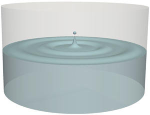
Figure 3 shows a cylindrical container of radius  $\hat {R}_0$ containing fluid whose surface is perturbed in the form of a Bessel mode. The displacement of the perturbed surface is measured from the flat undisturbed level and is given initially by
  $\hat {\eta }(\hat {r},0) = a_0{\textrm{J}}_0(k\hat {r}) = a_0{\textrm{J}}_0(({l_q}/{\hat {R}_0})\hat {r})$ where
  ${\textrm{J}}_0$ is the zeroth-order Bessel function of first kind and
  $l_q$ is explained below (2.6a,b). Surface oscillations arise due to the initial perturbation, and for a sufficiently large value of
  $\epsilon \equiv a_0({l_q}/{\hat {R}_0})$ (the precise value depends on the non-dimensional number
  $\sigma$), a jet is formed at the axis of symmetry towards the end of a surface oscillation. We study the IVP corresponding to this surface perturbation under the inviscid, irrotational approximation. Here we assume the liquid to be water and the gas above it to be air. Due to the large density ratio between the two, we may safely ignore the dynamic effect of air assuming that it exerts negligible pressure on the water surface. Thus the interface is treated as a free surface with a pressure jump across it due to surface tension.

Figure 3. Three-dimensional visualisation of surface perturbation (grey). Surface perturbation imposed at  $\hat {t}=0$ leads to a jet at the end of one oscillation for sufficiently large
  $\epsilon$. The coordinate system is centred at the axis of symmetry and
  $\hat {z}$ is measured from the unperturbed free surface.
The Laplace equation along with the nonlinear boundary conditions (kinematic boundary condition (2.2) and the Bernoulli equation with surface tension (2.3)) at the free surface and the mass conservation condition (2.4) govern the perturbation velocity potential and the perturbed interface. Equations for these are
 \begin{gather} \hat{\boldsymbol{\nabla}}\boldsymbol{\cdot}\hat{\boldsymbol{\nabla}}\hat{\phi} = 0, \end{gather}
 \begin{gather}\frac{\textrm{D}\hat{\eta}}{\textrm{D}\hat{t}} - \left(\hat{\boldsymbol{\nabla}}\hat{\phi}\boldsymbol{\cdot}\boldsymbol{e}_{\hat{z}}\right)_{\hat{z}=\hat{\eta}}=0, \end{gather}
 \begin{gather}\left(\frac{\partial\hat{\phi}}{\partial \hat{t}} + \frac{1}{2}|\hat{\boldsymbol{\nabla}}\hat{\phi}|^2 + g\hat{z} + \frac{T}{\rho}\hat{\boldsymbol{\nabla}}\boldsymbol{\cdot}\boldsymbol{n}\right)_{\hat{z}=\hat{\eta}} = 0, \end{gather}
 \begin{gather}\int_{0}^{\hat{R}_0}\hat{r}\hat{\eta}(\hat{r},\hat{t}) \,\textrm{d}\hat{r} = 0 , \end{gather}
where  $T$ is the coefficient of surface tension,
  $\boldsymbol {e}_{\hat {z}}$ and
  $\boldsymbol {n}$ are unit normals to the unperturbed and perturbed free surface, respectively, and
  $\hat {\boldsymbol {\nabla }}$ is the gradient operator to be expressed in axisymmetric, cylindrical coordinates. We propose to solve the nonlinear IVP for (2.1), (2.2) and (2.3) up to
  $O(\epsilon ^2)$ in cylindrical coordinates with an imposed surface perturbation (see figure 3 and (2.6a,b)). Appropriate boundary conditions are imposed on the velocity potential
  $\hat {\phi }$ at the axis of symmetry (
 $\hat {r}=0$) and the wall of the container at
  $\hat {r}=\hat {R}_0$ (no-penetration). In addition, we impose symmetry conditions on the free-surface at
  $\hat {r}=0$ as well as the free-end edge boundary condition at
  $\hat {r}=\hat {R}_0$ through (2.5a,b);
 \begin{gather} \left(\frac{\partial \hat{\phi}}{\partial \hat{r}}\right)_{\hat{r} = 0} = \left(\frac{\partial \hat{\phi}}{\partial \hat{r}}\right)_{\hat{r} = \hat{R}_0} = 0,\quad \left(\frac{\partial\hat{\eta}}{\partial\hat{r}}\right)_{\hat{r}=0} = \left(\frac{\partial\hat{\eta}}{\partial\hat{r}}\right)_{\hat{r}=\hat{R}_0}=0, \end{gather}
 \begin{gather}\hat{\eta}(\hat{r},0) = a_0{\textrm{J}}_0\left(\frac{l_q}{\hat{R}_0}\hat{r}\right),\quad \frac{\partial\hat{\eta}}{\partial \hat{t}}(\hat{r},0) = 0, \quad \hat{\phi}(\hat{r},\hat{z},0) = 0 \end{gather}
In (2.6a,b),  $l_q$ belongs to the set of (non-trivial) zeroes of
  ${\textrm{J}}_1(\cdot )$ with
  $q=1,2,3\ldots$, i.e.
  ${\textrm{J}}_1(l_q)=0$. This choice ensures that the initial condition satisfies (2.5a,b). For ease of algebra, we operate on (2.3) by
  ${\textrm {D}}/{\textrm {D}\hat {t}}$ replacing
  $\hat {\eta }$ in the gravity term with derivatives of
  $\hat {\phi }$ using (2.2) (Penney et al. Reference Penney, Price, Martin, Moyce, Penney, Price and Thornhill1952). In further calculations, we replace the kinematic boundary condition (2.2) with this equation. The resulting equations are then written in cylindrical axisymmetric coordinates ((1.1)–(1.6) in accompanying supplementary material available at https://doi.org/10.1017/jfm.2020.851) and non-dimensionalised using
 \begin{equation} r = \frac{l_q\hat{r}}{\hat{R}_0}, \quad z = \frac{l_q\hat{z}}{\hat{R}_0}, \quad t = {\left( \frac{gl_q}{\hat{R}_0} \right)}^{1/2}\hat{t}, \quad \eta = \frac{l_q\hat{\eta}}{\hat{R}_0} \quad \text{and}\quad \phi = {\left( \frac{l_q^3}{g\hat{R}_0^3} \right)}^{1/2} \hat{\phi}. \end{equation}
This leads to the following set:
 \begin{align} &\frac{\partial^2\phi}{\partial r^2} + \frac{1}{r}\frac{\partial\phi}{\partial r} + \frac{\partial^2\phi}{\partial z^2} = 0, \end{align}
 \begin{align} & \left(\frac{\partial^{2} \phi}{\partial t^{2}} + \frac{\partial \phi}{\partial z} + \left\{ \frac{\partial}{\partial t} + \frac{1}{2}\left( \frac{\partial \phi}{\partial r} \right) \frac{\partial}{\partial r} + \frac{1}{2}\left( \frac{\partial \phi}{\partial z} \right) \frac{\partial}{\partial z} \right\} {|\boldsymbol{\nabla}\phi|}^{2} \right )_{z=\eta} \nonumber\\ &\quad -\sigma\left\lbrace\left[\frac{\partial}{\partial t} + \left(\frac{\partial\phi}{\partial r}\right)_{z=\eta}\frac{\partial}{\partial r}\right]\left(\frac{\dfrac{\partial^2\eta}{\partial r^2}}{\left\{1 + \left(\dfrac{\partial \eta}{\partial r}\right)^2\right\}^{3/2}} + \dfrac{1}{r}\dfrac{\dfrac{\partial\eta}{\partial r}}{\left\{1 + \left(\dfrac{\partial \eta}{\partial r}\right)^2\right\}^{1/2}}\right)\right\rbrace = 0, \end{align}
 \begin{gather} \left(\frac{\partial \phi}{\partial t} + \frac{1}{2}{ {| \boldsymbol{\nabla} \phi |}^2} + z\right)_{z=\eta} - \sigma\left(\frac{\dfrac{\partial^2\eta}{\partial r^2}}{\left\{1 + \left(\dfrac{\partial \eta}{\partial r}\right)^2 \right\}^{3/2}} + \frac{1}{r}\frac{\dfrac{\partial\eta}{\partial r}}{\left\{1 + \left(\dfrac{\partial \eta}{\partial r}\right)^2\right\}^{1/2}}\right) = 0, \end{gather}
 \begin{gather}\int_{0}^{l_q} r \eta(r,t) \,\textrm{d}r = 0, \end{gather}
 \begin{gather} \left(\frac{\partial \phi}{\partial r}\right)_{r = 0} = \left(\frac{\partial \phi}{\partial r}\right)_{r = l_q} = 0,\quad \left(\frac{\partial\eta}{\partial r}\right)_{r=0} = \left(\frac{\partial\eta}{\partial r}\right)_{r=l_q}=0 , \end{gather}
 \begin{gather} \text{and}\quad \eta(r,0) = \epsilon{\textrm{J}}_0(r),\quad \frac{\partial\eta}{\partial t}(r,0) = 0, \quad\phi(r,z,0) = 0, \end{gather}
Equations (2.8)–(2.13a–c) contain two non-dimensional groups viz. the nonlinearity parameter  $\epsilon \equiv a_0({l_q}/{\hat {R}_0})$ and
  $\sigma \equiv {T({l_q}/{\hat {R}_0})^2}/{\rho g}$ which measures the relative strength of surface tension to gravity and is the inverse of Bond number. Note that
  $\epsilon$ appears in the initial condition while
  $\sigma$ appears in the boundary condition. It is important to remember in further analysis that
  $q$ is a fixed integer serving as an index for the primary mode. In this study
  $q$ has been chosen to be
  $5$, to remain consistent with the deep water approximation treated here. We treat
  $\epsilon$ as a small parameter with
  $\sigma = O(1)$ expanding
  $\phi$,
  $\eta$ and
  $t$ in (2.8)–(2.12a,b) as
 \begin{gather} \phi(r,z,t) = 0 + \epsilon\phi_1(r,z,t) + \epsilon^2\phi_2(r,z,t) + \epsilon^3\phi_3(r,z,t) + O(\epsilon^4), \end{gather}
 \begin{gather}\eta(r,t) = 0 + \epsilon\eta_1(r,t) + \epsilon^2\eta_2(r,t) + \epsilon^3\eta_3(r,t) + O(\epsilon^4), \end{gather}
 \begin{gather}\tau = t\left[1 + \epsilon^2 \varOmega_2 + O(\epsilon^3)\right]. \end{gather}
The expansion of  $t$ in (2.16) is a standard Lindstedt–Poincaré technique and is necessary in order to take into account the nonlinear dependence of the oscillation frequency on the amplitude
  $\epsilon$ of the Bessel modes. Substituting (2.14)–(2.16) into (2.8)–(2.13a–c) and using Taylor series expansions about
  $z=0$, we may generically write at any
  $O(\epsilon ^i)$ (
 $i=1,2,3,\ldots$)
 \begin{gather} \frac{\partial^2\phi_i}{\partial r^2} + \frac{1}{r}\frac{\partial\phi_i}{\partial r} + \frac{\partial^2\phi_i}{\partial z^2} = 0, \end{gather}
 \begin{gather}\left(\frac{\partial^2\phi_i}{\partial \tau^2} + \frac{\partial \phi_i}{\partial z}\right)_{z=0} - \sigma\left[ \left(\frac{\partial^3 \eta_i}{\partial \tau \partial r^2}\right) + \frac{1}{r} \left(\frac{\partial ^2 \eta_i}{\partial \tau \partial r} \right) \right] = G_i(r,\tau), \end{gather}
 \begin{gather}\left(\frac{\partial \phi_i}{\partial \tau}\right)_{z=0} + \eta_i - \sigma\left[\left(\frac{\partial^2 \eta_i}{\partial r^2}\right) + \frac{1}{r} \left(\frac{\partial \eta_i}{\partial r}\right)\right] = F_i(r,\tau), \end{gather}
 \begin{gather}\int_{0}^{l_q} r \eta_i(r,t)\,\textrm{d}r = 0, \end{gather}
 \begin{gather} \left(\frac{\partial \phi_i}{\partial r}\right)_{r = 0} = \left(\frac{\partial \phi_i}{\partial r}\right)_{r = l_q} = 0,\quad \left(\frac{\partial\eta_i}{\partial r}\right)_{r=0} = \left(\frac{\partial\eta_i}{\partial r}\right)_{r=l_q}=0, \end{gather}
 \begin{gather} \eta_i(r,0) = {\textrm{J}}_0(r)\delta_{1i}, \quad \frac{\partial\eta_i}{\partial \tau}(r,0) = \phi_i(r,z,0)=0, \end{gather}
where  $\delta _{ij}$ is the Kronecker delta. As is usual in perturbative methods, the only difference at different orders in (2.18) and (2.19) are the expressions
  $F_i$ and
  $G_i$ on the right-hand side. Here
  $F_1(r,\tau ) = G_1(r,\tau ) = 0$ while
  $F_2(r,\tau ),G_2(r,\tau ), F_3(r,\tau ), G_3(r,\tau )$ have lengthy expressions provided in appendix A. Our task is to now solve (2.17)–(2.22a,b) up to
  $i=2$ (second order). Note that for determining the solution up to
  $i=2$ completely, it is necessary to also obtain the equations at
  $i=3$.
Observe that  $\phi (r,z,\tau )=p(\tau ){\textrm{J}}_0(\alpha r)\exp [\alpha z]$ satisfies the axisymmetric Laplace equation (2.17) for any (real)
  $\alpha$ and
  $p(\tau )$. In addition, if we choose
  $\eta (r,\tau ) = a(\tau ){\textrm{J}}_0(l_j({r}/{l_q}))$ and
  $\phi (r,z,\tau ) = p(\tau ){\textrm{J}}_0(l_j({r}/{l_q}))\exp (l_j({z}/{l_q}))$, the identity
  $\int _{0}^{l_q}{\textrm{J}}_0(l_j ({r}/{l_q})) r \,\textrm {d}r = 0$ and the equation
  ${\textrm{J}}_1(l_j)=0$
  $\forall j \in \mathbb {Z}^{+}$ ensure that (2.20) and (2.21a,b) are also satisfied. Thus the general solution for
  $\phi _i$ and
  $\eta _i$ satisfying (2.17) and conditions (2.20) and (2.21a,b) may be posed as an eigenfunction expansion (Dini series, Mack Reference Mack1962)
 \begin{gather} \phi_i(r,z,\tau) = \sum_{j = 0}^{\infty} p_{i}^{(\,j)}(\tau) {\textrm{J}}_0\left(\alpha_j r\right) \exp\left(\alpha_j z\right), \end{gather}
 \begin{gather}\eta_i(r,\tau) = \sum_{j = 0}^{\infty} a_{i}^{(\,j)}(\tau) {\textrm{J}}_0\left(\alpha_j r\right)\quad \text{with} \ \alpha_j \equiv \frac{l_j}{l_q}. \end{gather}
Substituting (2.23) and (2.24) into (2.18) and (2.19) and using orthogonality relations among Bessel functions (see supplementary material), we obtain the following equations governing the coefficients  $p_i^{m}(\tau )$ and
  $a_i^{m}(\tau )$ at any order
  $O(\epsilon ^i)$:
 \begin{gather} \frac{\textrm{d}^2p_{i}^{(m)}}{\textrm{d}\tau^2} + \omega_{m}^2p_{i}^{(\,j)}(\tau) = \left(1 + \sigma\alpha_m^2\right)\mathbb{G}_i^{(m)}(\tau) - \sigma\alpha_m^2\frac{\textrm{d} \mathbb{F}_i^{(m)}}{\textrm{d}\tau}, \end{gather}
 \begin{gather}a_i^{(m)}(\tau) = \frac{1}{1 + \sigma\alpha_m^2}\left(\mathbb{F}_i^{(m)}(\tau) - \frac{\textrm{d}p_i^{(m)}}{\textrm{d}\tau}\right),\quad m=0,1,2\ldots\,. \end{gather}
Here  $\omega _m^2 \equiv \alpha _m(1 + \sigma \alpha _m^2)$ is the deep-water linear dispersion relation for capillary-gravity waves written in scaled variables.
  $\mathbb {F}_i^{(m)}(\tau )$ and
  $\mathbb {G}_i^{(m)}(\tau )$ in (2.25) and (2.26) are defined as
 \begin{equation} \left.\begin{gathered} \mathbb{G}_i^{(m)}(\tau) \equiv\frac{2}{l_q^2{\textrm{J}}_0^2\left(l_m\right)}\int_{0}^{l_q} \textrm{d}r r {\textrm{J}}_0\left(\alpha_m r\right) G_i(r,\tau), \\ \mathbb{F}_i^{(m)}(\tau) \equiv \frac{2}{l_q^2{\textrm{J}}_0^2\left(l_m\right)}\int_{0}^{l_q} \textrm{d}r r {\textrm{J}}_0\left(\alpha_m r\right) F_i(r,\tau). \end{gathered}\right\}\end{equation}
Equation (2.25) may now be solved for  $p_i^{(m)}(\tau )$ (with suitable initial conditions) and the resultant solution determines
  $a_i^{(m)}(\tau )$ using (2.26). With
  $m=0,1,2,3\ldots$ and
  $i=1,2,3\ldots \,$, the initial conditions from (2.22a,b) are
 \begin{gather} p_i^{(m)}(0) = 0,\quad \frac{\textrm{d}p_i}{\textrm{d}\tau}^{(m)}(0) = \mathbb{F}_i^{(m)}(0) - \left( 1 + \sigma\alpha_m^2 \right) \delta_{mq}\delta_{i1}, \end{gather}
 \begin{gather}a_i^{(m)}(0) = \delta_{mq}\delta_{i1},\quad\frac{\textrm{d}a_i^{(m)}}{\textrm{d}\tau}(0) = 0. \end{gather}
We determine  $p_i^{m}(\tau )$ and
  $a_i^{m}(\tau )$ using (2.25) and (2.26), respectively, at various orders using initial conditions (2.28a,b) and (2.29a,b).
2.2. Linear solution:  $O(\epsilon )$

At  $O(\epsilon )$, the solution is elementary. It is shown in the accompanying supplementary material that at linear order, the only non-zero term in the eigenfunction expansion in (2.23) and (2.24) is for
  $j=q$, the primary mode. With
  $\omega _q^2 = 1 + \sigma$, this leads to,
 \begin{equation} \phi_1(r,z,\tau) ={-}\omega_q\sin(\omega_q\tau){\textrm{J}}_0(r)\exp\left(z\right) ,\quad \eta_1(r,\tau) = \cos(\omega_q\tau){\textrm{J}}_0(r). \end{equation}
2.3. Nonlinear corrections: $O(\epsilon ^2)$

At  $O(\epsilon ^2)$, the calculation is algebraically tedious and quite lengthy, but otherwise standard. We outline the key results below, referring the interested reader to the accompanying supplementary material for the detailed derivation. Using (2.23) and (2.24), we obtain at
  $O(\epsilon ^2)$,
 \begin{align} \eta_{2}(r,\tau) &= \sum_{k = 1}^{\infty}\left[\zeta_1^{(k)}\cos(\omega_{k}\tau) + \zeta_2^{(k)}\cos(2\omega_{q}\tau) + \zeta_3^{(k)} \right]{\textrm{J}}_0(\alpha_k r) , \end{align}
 \begin{align} \phi_2(r,z,\tau) &= \frac{{\textrm{J}}_0^2(l_q)}{2}\sin\left(2\omega_q\tau\right) \nonumber\\ &\quad + \sqrt{1+\sigma}\sum_{k=1}^{\infty}\left[\xi^{(k)}_1\sin\left(\omega_k\tau\right) + \xi^{(k)}_2\sin\left(2\omega_q\tau\right)\right]{\textrm{J}}_0 \left(\alpha_k r\right)\exp\left(\alpha_k z\right), \end{align}
where expressions for  $\zeta _1^{(k)},\zeta _2^{(k)},\zeta _3^{(k)}$ and
  $\xi _1^{(k)}, \xi _2^{(k)}$ are provided in appendix B. Note the presence of terms in (2.31) and (2.32), which are pure functions of space and time, respectively. This implies that there is a nonlinear correction to the (temporal) mean interface level, note the third term in (2.31) whose time average is non-zero. Similarly there is a nonlinear correction in
  $\phi$ whose spatial average is non-zero. An important thing to note in the nonlinear solution (2.31) and (2.32) is the presence of the entire spectrum (and not just the
  $q$th primary mode) at this order, which implies a nonlinear transfer of energy to the entire spectrum. This transfer of energy will be seen to be crucial to jetting.
Despite having expressions for  $\phi (r,z,\tau )$ and
  $\eta (r,\tau )$ up to
  $O(\epsilon ^2)$, our calculation is incomplete, as a nonlinear correction to the dispersion relation
  $\omega_m^2 = \alpha_m(1+ \alpha_m^2\sigma)$
 $[1 + O(\epsilon^2)]$ is expected at this order, through
  $\varOmega _2$ in (2.16). For determining this, it is necessary to proceed to the third order (
 $O(\epsilon ^3)$) where elimination of resonant forcing of the primary mode (subscript
  $q$) will determine this correction. We emphasise that we do not determine the
  $O(\epsilon ^3)$ corrections to
  $\phi (r,z,\tau )$ and
  $\eta (r,\tau )$. A minimal
  $O(\epsilon ^3)$ calculation is carried out for determining
  $\varOmega _2$. This is done by obtaining the equations governing
  $p_3^{(m)}(\tau )$ and setting the coefficient of the resonant forcing term (for the primary mode) to zero. In this way, we obtain after some lengthy algebraic manipulations (see supplementary material)
 \begin{align} \varOmega_2 &= \frac{1}{2{\textrm{J}}_0^2(l_q)}\left[ \sum_{l = 1}^{\infty} \left[ \left\{\left[\alpha_l\left(2 + \sigma\right) - \alpha_l^2\right]\xi_2^{(l)} + 2\sigma\zeta_2^{(l)}\right\}{{I}}_{0 - l, 0- q, 0 - q}\right.\right.\nonumber\\ &\quad \left. - \left\{ 2\left(1 + \sigma\right)\alpha_l\xi_2^{(l)} + {\alpha_l^3\sigma}\zeta_2^{(l)} - 2\alpha_l^3\sigma\zeta_3^{(l)} \right\}{{I}}_{0 - q, 1 - q , 1 - l}\right] \nonumber\\ &\quad - \frac{\left(1 + \sigma\right)}{2}{{I}}_{0 - q, 0- q,0 - q, 0- q} + \frac{\left(1 - 4\sigma + \sigma^2\right)}{4\left(1 + \sigma\right)}{{I}}_{0 - q,0 - q, 1 - q, 1- q} \nonumber\\ &\quad \left. + \frac{3\left(1 + 3\sigma + \sigma^2 \right)}{4\left(1 + \sigma\right)}{{I}}_{0 - q, 1 - q, 1- q, 2 - q} \right]. \end{align}
Note that as shorthand notation in (2.33) we have used
 \begin{equation} {{I}}_{\nu_1- m_1, \nu_2- m_2,\ldots} \equiv \int_{0}^{1} \textrm{d}\tilde{r} \,\tilde{r}\, {\textrm{J}}_{\nu_1}\left(l_{m_1}\tilde{r}\right){\textrm{J}}_{\nu_2}\left(l_{m_2}\tilde{r}\right)\ldots \end{equation}
where  $\tilde {r} \equiv r/l_q$ and
  $\nu _i,m_i = 0,1,2,\ldots$, e.g.
 \begin{equation} {{I}}_{0- m,1- q,1- q} \equiv \int_{0}^{1} \,\textrm{d}\tilde{r}\,\tilde{r}\,{\textrm{J}}_{0}\left(l_m\tilde{r}\right){\textrm{J}}_{1}^2\left(l_q\tilde{r}\right). \end{equation}
With  $\sigma =1.086$ and parameters corresponding to air–water (see table 3), the amplitude correction to the dispersion relation for the primary mode
  $q=5$ evaluates to
  $\varOmega _2 \approx -0.0332$, using expression (2.33).
2.4. Summary of weakly nonlinear theory
We may now combine results up to  $O(\epsilon ^2)$ to predict
 \begin{align} \eta(r,\tau) &= \epsilon{\textrm{J}}_0(r)\cos\left(\omega_q \tau\right) + \epsilon^2\sum_{k=1}^{\infty}\left[\zeta_1^{(k)}\cos\left(\omega_k\tau\right) + \zeta_2^{(k)}\cos\left(2\omega_q\tau\right) + \zeta_3^{(k)}\right]{\textrm{J}}_0\left(\alpha_k r\right) \nonumber\\ &\quad + O(\epsilon^3), \end{align}
 \begin{align} \phi(r,z,\tau) &={-}\epsilon \omega_q {\textrm{J}}_0(r)\exp\left(z\right)\sin\left(\omega_q\tau\right) + \epsilon^2 \frac{{\textrm{J}}_0^2(l_q)}{2}\sin\left(2\omega_q\tau\right) \nonumber\\ &\quad + \epsilon^2\sqrt{1+\sigma}\sum_{k=1}^{\infty}\left[ \xi^{(k)}_1\sin\left(\omega_k\tau\right) + \xi^{(k)}_2\sin\left(2\omega_q\tau\right) \right] {\textrm{J}}_0\left(\alpha_k r\right)\exp\left(\alpha_k z\right) + O(\epsilon^3) \end{align}
 \begin{align} \text{and}\quad \omega_k^2 &= \alpha_k\left(1+\sigma\alpha_k^2\right)\left[1+\epsilon^2\varOmega_2 + O(\epsilon^3)\right], \end{align}
where  $\varOmega _2$ is given by (2.33). It may be checked that (2.36) and (2.37) satisfy the initial conditions (2.13a–c). In particular
  $\zeta _1^{(k)} + \zeta _2^{(k)} + \zeta _3^{(k)} =0$ for all
  $k=1,2\ldots$ which ensures that
  $\eta (r,0) = \epsilon {\textrm{J}}_0(r)$. Other initial conditions in (2.13a–c) involving the time derivative of
  $\eta (r,t)$ and on
  $\phi (r,z,0)$ are trivially verified. The singularity of the expressions for
  $\xi _1^{(k)}, \xi _2^{(k)}$, etc. at a possible
  $\omega _k = 2\omega _q$ is discussed further in § 6. As (2.36) and (2.37) are an infinite series, we truncate them for numerical evaluation in later sections. For any
  $r$,
$r$,  $z$ and
  $\tau$, it may be expected that the infinite sums in (2.36) and (2.37) have progressively smaller contributions at higher values of
  $k$. This is seen in figures 4(a) and 4(b) where we have evaluated the coefficients
  $\zeta _1^{(k)},\zeta _2^{(k)},\zeta _3^{(k)}$ and
  $\xi _1^{(k)},\xi _2^{(k)}$ for the primary mode
  $q=5$ as a function of
  $k$ in (2.36) and (2.37). It is seen that the peak values are at around
  $k=10$ which is expected, as this is the second multiple of
  $q=5$ and our calculation is accurate up to
  $O(\epsilon ^2)$. Thus for
  $q=5$, one needs to retain at least 10 terms while numerically evaluating the infinite series (2.36) and (2.37). For high accuracy, we have retained the first
  $85$ terms in our expansions. All the integrals that appear in
  $\zeta _1^{(k)}, \zeta _2^{(k)}\ldots$ have been evaluated numerically using MATLAB (MAT 2018).


3. Numerical simulations
In this section, we provide a brief description of the code used for numerical simulations of the incompressible Euler equation with surface tension supplemented with an equation for tracking the interface, viz. (3.1a,b) and (3.2). The simulations have been performed using the open-source code Basilisk (Popinet Reference Popinet2020), a successor to the well-known open-source solver Gerris (Popinet Reference Popinet2003, Reference Popinet2009). These codes have been carefully benchmarked on a suite of interfacial flow problems over many years and results using these have extensively appeared in the literature, e.g. Agbaglah et al. (Reference Agbaglah, Delaux, Fuster, Hoepffner, Josserand, Popinet, Ray, Scardovelli and Zaleski2011), Dasgupta, Tomar & Govindarajan (Reference Dasgupta, Tomar and Govindarajan2015), Farsoiya et al. (Reference Farsoiya, Mayya and Dasgupta2017), Fuster & Popinet (Reference Fuster and Popinet2018), Deike et al. (Reference Deike, Ghabache, Liger-Belair, Das, Zaleski, Popinet and Séon2018), Lai et al. (Reference Lai, Eggers and Deike2018), Singh, Farsoiya & Dasgupta (Reference Singh, Farsoiya and Dasgupta2019), Blanco-Rodríguez & Gordillo (Reference Blanco-Rodríguez and Gordillo2020) and Dhar, Das & Das (Reference Dhar, Das and Das2020), to mention only a small set. Basilisk implements the finite-volume algorithm using the Bell–Collela–Glaz (Bell, Colella & Glaz Reference Bell, Colella and Glaz1989) advection scheme. A semi-implicit scheme is utilised to calculate velocity and pressure fields. For capturing the interface, the geometric volume of fluid method (Scardovelli & Zaleski Reference Scardovelli and Zaleski1999) is used along with the continuum surface force model for including surface tension as a body force into the momentum equations (Brackbill, Kothe & Zemach Reference Brackbill, Kothe and Zemach1992; Popinet Reference Popinet2018). An important point to note in the context of the present study is that Basilisk implements the one-fluid model, and hence necessarily solves for both air and water. In contrast, the weakly nonlinear analysis described earlier ignores the inertial effect of air, assuming it to be a relatively low density gas compared with water. Thus, when comparing our numerical simulations, minor differences are expected between theory and simulations near the interface;
 \begin{gather} \boldsymbol{\nabla}\boldsymbol{\cdot}\boldsymbol{u} = 0,\quad \frac{\partial\boldsymbol{u}}{\partial t}+\boldsymbol{\nabla}\boldsymbol{\cdot} (\boldsymbol{u}\otimes\boldsymbol{u}) ={-}\frac{1}{\rho}\boldsymbol{\nabla} p + \boldsymbol{g} + \frac{T}{\rho} \kappa \delta_s \boldsymbol{n}, \end{gather}
 \begin{gather} \frac{\partial f}{\partial t} + \boldsymbol{\nabla}\boldsymbol{\cdot}(f \boldsymbol{u}) = 0.\end{gather}
In (3.1a,b) and (3.2),  $\boldsymbol {u}$,
  $p$,
$p$,  $T$,
$T$,  $\kappa$ and
  $f$ are velocity, pressure, surface tension coefficient, curvature and volume fraction fields, respectively. The computational box is depicted in figure 5 with boundary conditions in table 2. Note that boundary
  $\# 1$ in figure 5 is the axis of symmetry. Parameters for the simulations are reported in table 3. Case
  $9$ in table 3 represent a set of numerical simulations used for scaling analysis. The parameters for these are numerous and listed in the accompanying supplementary material. Note that some of the simulations for this case deviate from air–water parameters with respect to surface tension. The density of air (in the centimetre–gram–second system of units ) has been chosen to be
  $0.001$. Simulations are done with uniform
  $1024\times 1024$ and
  $2048\times 2048$ grids and are tested for convergence, with grid refinement (see accompanying supplementary material). A repository with script files has been set up in Basak, Farsoiya & Dasgupta (Reference Basak, Farsoiya and Dasgupta2020), using which the results discussed below may be reproduced. The Basilisk script file is also provided as additional supplementary material.

Figure 5. Initial condition.
Table 2. Boundary conditions.

Table 3. Simulation parameters in the centimetre–gram–second system of units. Grid (a)  $1024\times 1024$; grid (b)
  $2048\times 2048$.

4. Results and analysis
We test theoretical predictions against numerical simulations here and provide detailed comparisons and analysis in the following subsections.
4.1. Tracking the interface at $r=0$

In figure 6, we show the time signals obtained by tracking the interface at  $r=0$. For
  $\epsilon =0.2$ in figure 6(a) a very good match is seen with the linearised theoretical predictions. Already at
  $\epsilon =0.5$ (figure 6b), visible differences appear with the linearised prediction. The insets in all panels in figure 6 depict the instantaneous shape of the interface at the time instant indicated by the arrow. In figures 6(c) and 6(d) we have plotted the signals for
  $\epsilon =1.2$ and
  $\epsilon =1.7$, respectively. While the agreement with theory is moderately good in figure 6(c), the linearised signal clearly shows a poor match. In figure 6(d), where
  $\epsilon = 1.7$, a slender jet is produced in numerical simulations ejecting a drop from its tip. Here the nonlinear theory significantly improves over the linear prediction but produces a somewhat broader jet without the droplet ejection at the tip, see inset. As seen in figures 6(c) and 6(d), at the end of one oscillation the height of the (scaled) interface at
  $r=0$ is significantly more than unity. This overshoot is a signature of jetting which the nonlinear theory manages to capture reasonably well. Another interesting feature seen in the upper insets of figures 6(b) and 6(c) is the appearance of a small dimple which is a known precursor to jet formation in other scenarios such as bubble bursting (Deike et al. Reference Deike, Ghabache, Liger-Belair, Das, Zaleski, Popinet and Séon2018; Gañán-Calvo Reference Gañán-Calvo2017). Note that this dimple already starts appearing as a broader structure during the earlier downward motion of the cavity and at that instant is well described by the nonlinear theory (bottom insets in figures 6b and 6c). This, however, gets smoothed out as the cavity reaches its lower extremity. Note that the abrupt drop in amplitude around
  $t\approx 3.8$ in figure 6(d) is due to ejection of a droplet. A point worth noting here is that for
  $\epsilon =1.2$, we see that the
  $O(\epsilon ^2)$ predictions work reasonably well (figure 6c) despite the fact that the theory is strictly valid only for
  $\epsilon < 1$. This is a recurrent situation in fluid dynamical problems involving a small parameter, e.g. in boundary layer theory the parallel flow assumption involves errors at least of
  $O(Re^{-1/3})$ (Govindarajan & Narasimha Reference Govindarajan and Narasimha1999; Govindarajan Reference Govindarajan2004). However, despite this it provides very good predictions for instability down to
  $Re < 10$, although the magnitude of the error is nearly an order-one number at these Re.

Figure 6. Motion of the interface at  $r=0$ with time
  $t$: (a)
  $\epsilon = 0.2 \ll 1$, no jetting in linear regime; (b) at moderately large
  $\epsilon =0.5$ interface shows dimple formation, see insets depicting instantaneous interface shape (
 $\eta /\epsilon$ versus
  $r$) at the data point indicated by arrow. Weakly nonlinear model captures the onset of dimple at
  $t \approx 1.228$ but does not describe it well later at
  $t\approx 3.133$ when it narrows and sharpens. Pronounced dimple and a clear overshoot (above unity) is observed in panel (c) for
  $\epsilon =1.2$. (d) For
  $\epsilon =1.7$, a slender jet with large overshoot and droplet ejection at the tip. While weakly nonlinear theory captures the qualitative features, linear theory is unable to describe any of these.
4.2. Comparison of interface shape
Comparisons of the interface shape as a function of time are provided in figures 7 and 8 for  $\epsilon =0.5$ and
  $\epsilon =1.2$, respectively. Significant nonlinear effects are manifested for a moderately large
  $\epsilon =0.5$ in figure 7. In figure 7(b), it is seen that at the instant when dimple formation commences, linear theory makes a large error near
  $r=0$, while a good match is seen with the weakly nonlinear theory. As the dimple shrinks in horizontal extent during the upward motion of the cavity in figure 7(d), the nonlinear theory captures the interface shape but does not capture the dimple. In the next few snapshots in figure 7(e–h), the nonlinear theory captures the time evolution accurately. Similarly for
  $\epsilon =1.2$ in figure 8, strong nonlinear effects are visible around
  $r=0$ in figure 8(b), and particularly in figure 8(c) as dimple formation commences. Here weakly nonlinear theory provides an accurate description. However, like in figure 7, the pronounced dimple and its time evolution involving thinning of the jet neck, are not well resolved by the nonlinear prediction as seen in figures 8(d) and 8(e). Interestingly, the nonlinear theory describes the shape well later in figure 8(g), capturing the extent of overshoot (over unity) at
  $r=0$ quite well. An important feature is that as
  $\epsilon$ is increased from
  $0.5$ to
  $1.7$ (comparison for
  $\epsilon =1.7$ is provided in the supplementary material), the width of the dimple decreases (see insets in figures 7d and 8d), while the speed at which the tip of the dimple rises upwards increases with increasing
  $\epsilon$. This may be inferred from the slope of the ascending part of the curve in figures 6(c) and 6(d).

Figure 7. (a–h) Comparison of the (non-dimensional) interface shape  $\eta /\epsilon$ versus radius
  $r$ at various (non-dimensional) time instants for
  $\epsilon = 0.5$: (a)
  $t=0$; (b)
  $t=1.228$; (c)
  $t=1.658$; (d)
  $t=3.133$; (e)
  $t=3.378$; (\,f)
  $t=3.685$; (g)
  $t=4.177$; (h)
  $t=4.607$. Simulation profiles (—, black), linear theory (
 $\square$, red) and weakly nonlinear theory (
 $\bullet$, blue). Dimple formation initiates in panel (b), is suppressed as the trough reaches its lowest point and reappears with significant shortening in scale as seen in inset of panel (d). Weakly nonlinear model qualitatively and significantly improves over the linearised model in this regime. For parameters, see case
  $1$ in table 3, grid (a).

Figure 8. (a–h) Comparison of the (non-dimensional) interface shape  $\eta /\epsilon$ versus radius
  $r$ at various (non-dimensional) time instants for
  $\epsilon = 1.2$: (a)
  $t=0$; (b)
  $t=1.228$ s; (c)
  $t=1.658$; (d)
  $t=3.071$; (e)
  $t=3.378$; (\,f)
  $t=3.685$; (g)
  $t=4.177$; (h)
  $t=4.607$. Simulation profiles (—, black) are compared with linear (
 $\square$, red) and weakly nonlinear predictions (
 $\bullet$, blue). Dimple initiation is well captured by the nonlinear theory in panel (c) but not later on in panel (d) where the dimple becomes sharper and more pronounced, see inset. The thinning of the neck of the jet is not captured by the nonlinear model in panel (e). Near maximum overshoot, the jet shape near
  $r=0$ is well described by theory, see panel (\,f,g). For parameters see case
  $5$ in table 3, grid (b).
4.3. Comparison of vertical velocity and pressure profiles
Comparisons of the vertical velocity profile at two instants of time are provided in figures 9(a) and 9(b). It is seen from figure 9(a) which corresponds to the pronounced dimple event, that a large vertical velocity develops at the base of the interface. An order-of-magnitude estimate of this velocity maybe obtained using the width of the dimple using the capillary velocity scale (Gordillo & Rodríguez-Rodríguez Reference Gordillo and Rodríguez-Rodríguez2019)  $\sqrt {{T}/{\rho W_{{dimple}}}}$, where
  $W_{{dimple}}=0.42$ cm is the dimple width. This yields a (scaled) capillary velocity estimate of around
  $0.814$ in good agreement with the maximum velocity seen in numerical simulations in figure 9(a). A good match of the velocity profile with nonlinear theory is seen in figure 9(a). Close to the instant of maximum interface height in figure 9(b), the velocity profile is almost zero everywhere except in a small region below the interface. In this region, the nonlinear theory predicts the qualitative profile correctly including the negative sign, although some details near the surface are not captured accurately. Note that linear theory predicts an incorrect sign, at this instant.

Figure 9. Comparison of (non-dimensional) vertical component of velocity  $u_z$ at the axis of symmetry (
 $r=0$) for
  $\epsilon =0.5$ at two time instants: (a)
  $\epsilon = 0.5$,
  $t=3.133$; (b)
  $\epsilon = 0.5$,
  $t=4.177$. Insets show the instantaneous interface shapes. (a) Vertical velocity profile when a pronounced dimple forms at the bottom of the trough. (b) Velocity profile around the time instant when the interface is at its maximum height. Note the qualitatively good agreement between the weakly nonlinear model and simulations in both cases, although the kinks in the profile are not captured by the nonlinear model. For parameters, see case
  $1$ in table 3, grid (a).
In figure 10, we show non-dimensional perturbation pressure profile  $P(r,z,t)$ at the axis of symmetry
  $r=0$ at various instants for
  $\epsilon =0.5$ (and
  $\epsilon =1.2$ in the supplementary material). The perturbation pressure field is calculated using
  $P(r,z,t)= -{\partial \phi }/{\partial t} - {1}/{2}|\boldsymbol {\nabla }\phi |^2$. The panels on the right-hand side in figure 10 are perturbation pressure contours from numerical simulations, and the insets show the instantaneous shape of the interface. The plots on the left-hand side show the pressure profile at
  $r=0$ as a function of the vertical coordinate
  $z$. It is seen clearly from these figures that the formation of the dimple is associated with a region of high positive pressure. When the weakly nonlinear theory is able to capture the onset of the dimple (
 $t=1.228$), the agreement between simulations and theory is very good, as verified from figure 10(a). However, at
  $t=3.133$ when the dimple shrinks in horizontal extent during the upward motion of the cavity, weakly nonlinear theory does not describe the dimple shape accurately and differences are seen between nonlinear theory and simulations especially close to the interface where an incorrect sign of pressure is predicted. It should be noted that an arbitrary shift has been carried out on the pressure data obtained from numerical simulations. This does not affect the conclusions as in the incompressible limit, only gradients of pressure are important.

Figure 10. Left panels: (non-dimensional) pressure profiles  $P(r,z,t)$ at the axis of symmetry
  $r=0$ at various time instants for
  $\epsilon =0.5$. Right panels: pressure contours from numerical simulations. The dashed line on the contour plots represents the depth of the unperturbed liquid at
  $t=0$. The insets depict the instantaneous interface shape. As the weakly nonlinear theory has been derived using a Taylor series expansion about the unperturbed state for the liquid side only, we plot data at most up to the (scaled) unperturbed depth (
 $z=9.6154$). For parameters, see case
  $1$ in table 3, grid (a). (a) Time
  $t=1.228$; pressure profiles (left) and contours (right) at the onset of dimple formation. (b) Time
  $t=3.133$; pressure profiles and contours with a sharper and narrower dimple. (c) Time
  $t=4.177$; pressure profiles and contours when the jet is close to its maximum height.
4.4. Jet overshoot analysis
In figure 11, we depict the interface towards the end of one oscillation. Only cases with larger values of  $\epsilon$ are shown, as in this regime the overshoot of the interface at
  $r=0$ above unity is pronounced with the maximum overshoot even exceeding
  $50\,\%$ (figure 11e). While the linear theory clearly does not have any overshoot, it is seen that nonlinear theory predicts an overshoot, albeit with varying accuracy. The extent of overshoot depends not only on
  $\epsilon$ but also on
  $\sigma$. This dependence is captured in figure 12 which plots the overshoot (
 $\hat {a}_{{max}} \equiv \hat {\eta }(0,t_{{max}})$) at the end of one oscillation as a function of
  $\epsilon$ at different values of
  $\sigma$. The extent of overshoot is seen to be a strong function of
  $\sigma$ as one may intuitively expect. This is because the emergence of the jet involves development of large curvature at the base (pronounced dimple). Surface tension has an opposing effect on this process, and thus for a given
  $\epsilon$ we expect that decreasing surface tension (decreasing
  $\sigma$) promotes jetting and thus overshoot. For moderate to large
  $\epsilon$, we have fitted the simulation data to an exponential profile of the form
  ${\hat {a}_{{max}}}/{a_0} = 1 + A(\sigma )\exp [B(\sigma )\epsilon ]$ with
  $A(\sigma ) \ll 1$. Note that for all
  $\sigma$, some data points numerically very close to unity have been removed as these cause
  $\ln [{\hat {a}_{{max}}}/{a_0}-1]$ to be undefined. The inset shows a reasonably good match to a straight line
  $y=x$ on a semi-log scale. The subplots on the right-hand side of figure 12 show the dependence of
  $A(\sigma )$ and
  $B(\sigma )$ on
  $\sigma$. Due to clustering of singularities in
  $\sigma$ in the analytical model (see discussion in § 6) in the range
  $0.02 \leq \sigma \leq 0.6$, it is not possible to compare analytical predictions of overshoot with simulation data in figure 12. To obtain this comparison, we choose
  $\sigma$ far away from these singularities viz.
  $\sigma =1.086$, consistent with our perturbation analysis which assumes that
  $\sigma = O(1)$. A comparison of the overshoot at the end of one oscillation predicted by the nonlinear expression (2.36) against simulation data is shown in figure 13(a). It is seen that there is approximately an 8 %–10 % difference in the extent of overshoot predicted by (2.36) to that seen in simulations, with the former overpredicting the extent of overshoot up to
  $\epsilon < 1.3$. In figure 13(b), we obtain the boundary demarcating the regime where
  ${<}10\,\%$ overshoot is observed in our simulations. Here too it is seen that increasing
  $\sigma$ requires one to go to increasingly higher values of
  $\epsilon$ in order to obtain overshoot and subsequent jetting.

Figure 11. The interface shape when the jet is at its maximum height towards the end of one oscillation, for various values of  $\epsilon$: (a)
  $\epsilon = 1.0, t=4.177$; (b)
  $\epsilon = 1.1, t=4.115$; (c)
  $\epsilon = 1.2, t=4.177$; (d)
  $\epsilon = 1.3, t=4.177$; (e)
  $\epsilon = 1.4, t=4.3$. Overshoot occurs when the scaled interface
  $\eta (r,t)/\epsilon$ exceeds unity and is always observed at
  $r=0$, the axis of symmetry. In the above figures, we show only the
  $\epsilon$ range where a sizeable overshoot (ranging from 7 %–51 %) is observed. Note that weakly nonlinear theory (blue dots) captures the interface shape and the maximum height quite well for all the cases seen here. For parameters see: (a) case
  $3$, (b) case
  $4$, (c) case
  $5$, (d) case
  $6$ and (e) case
  $7$ in table 3, grid (a) for all cases here. The percentage values for overshoot reported in each panel is calculated from data obtained from numerical simulations.

Figure 12. We define  $\hat {a}_{{max}} \equiv \hat {\eta }(0,t_{{max}})$ where
  $t_{{max}}$ is the instant when the jet reaches it maximum height. (a) Variation of
  ${\hat {a}_{{max}}}/{a_0}$ with
  $\epsilon$ for various values of
  $\sigma$ (see legend), from numerical simulations. For moderate to large values of
  $\epsilon$, the inset shows an approximate data collapse using the empirical relation
  ${\hat {a}_{{max}}}/{a_0} = 1 + A(\sigma )\exp [B(\sigma )\epsilon ]$. Note that
  $A(\sigma ) \ll 1$ which ensures that
  ${\hat {a}_{{max}}}/{a_0}\approx 1$ as
  $\epsilon \rightarrow 0$.

Figure 13. (a) Comparison of the variation of overshoot given by  $({\hat {a}_{{max}}}/{a_0})$ with
  $\epsilon$ for
  $\sigma =1.086$,
  $A(\sigma ) =1.562\times 10^{-4}$ and
  $B(\sigma ) =5.8864$. It is seen that the weakly nonlinear theory (blue symbols) follows the qualitative trend seen in numerical simulations (black symbols). The solid (pink) line is
  ${\hat {a}_{{max}}}/{a_0} = 1 + A(\sigma )\exp [B(\sigma )\epsilon ]$ where the values of
  $A$ and
  $B$ are provided in the captions. (b) Simulation data. The curve is obtained from simulations and separates points where
  ${>}10\,\%$ overshoot is observed from those with
  ${<}10\,\%$ overshoot. It is clear from this curve that a higher value of
  $\epsilon$ is needed for jetting as surface tension is made stronger relative to gravity.
5. Energy and modal analysis
For our system, the total energy is a conserved quantity. Due to truncation of higher-order terms, the weakly nonlinear approximation does not conserve energy exactly and the fluctuations are quantified here. As shown in Zakharov (Reference Zakharov1968) and Segur & Stewart (Reference Segur and Stewart2020), the depth averaged total energy per unit horizontal surface area  $\rho \hat {E}_{{tot}}(\hat {r},\hat {t})$, is defined as
 \begin{align} \frac{\hat{E}_{{tot}}}{g \left(\dfrac{\hat{R}_0}{l_q}\right)^2} &\equiv E_{{tot}}(r,t) = E_{{kin}} + E_{{pot}} \nonumber\\ &= \int_{-\infty}^{\eta} \tfrac{1}{2}{|\boldsymbol{\nabla}\phi| }^2\,\textrm{d}z + \tfrac{1}{2}\eta^2 + \sigma\left({\sqrt{1 + {|\boldsymbol{\nabla}_{{\boldsymbol{H}}}\,\eta|}^2 }} - 1\right). \end{align}
Here  $E_{{tot}}(r,t)$ satisfies the conservation equation
  ${\partial E_{{tot}}}/{\partial t} + \boldsymbol {\nabla }_{{\boldsymbol {H}}}\boldsymbol {\cdot }\boldsymbol {F} = 0$ with the energy flux defined as
  $\mathcal {{\boldsymbol {F}}}(r,t) \equiv -\int _{-\infty }^{\eta }(\boldsymbol {\nabla }_{{\boldsymbol {H}}}\,\phi ) ({\partial \phi }/{\partial t}) \,\textrm {d}z - \sigma [{{\partial \eta }/{\partial t}(\boldsymbol {\nabla }_{{\boldsymbol {H}}}\,\eta ) }/{\sqrt {1 + {| \boldsymbol {\nabla }_{{\boldsymbol {H}}}\,\eta |}^2 }}]$.
With  $\boldsymbol {\nabla }_{{\boldsymbol {H}}} \equiv \boldsymbol {e}_r{\partial }/{\partial r}$ and
  $\boldsymbol {\nabla } \equiv (\boldsymbol {\nabla }_{{\boldsymbol {H}}},{\partial }/{\partial z})$ and integrating the energy per unit area in (5.1) over the entire horizontal surface area, with the two-dimensional divergence theorem, we see that
  $\boldsymbol {F}(l_q,t)=0$ due to boundary conditions at the radial wall. We thus obtain the energy conservation condition
  ${\textrm {d}\mathcal {E}}/{\textrm {d}t} \equiv {\textrm {d}}/{\textrm {d}t}(\int _{0}^{l_q}E(r,t)r\,\textrm {d}r)=0$. At the linearised approximation,
  $E(r,t)$ has quadratic terms in
  $\epsilon$ whence it may be checked that
  $\mathcal {E}$ is a constant. In figure 14(a), we show comparisons of the potential energy (gravitational potential energy plus the surface energy) of the system as a function of time (
 $\mathcal {E}_0$ is the initial value of potential or total energy under each approximation) and a good agreement is seen, including that at the instant when the dimple becomes pronounced. In figure 14(b), we see the variation of total energy. Due to the truncation of
  $O(\epsilon ^3)$ terms, the weakly nonlinear model does not conserve energy exactly and the oscillatory nature of these fluctuations is because we solve simple harmonic oscillator equations at every order. Figures 14(a) and 14(b) together imply that the weakly nonlinear model estimates the surface energy relatively more accurately than the kinetic energy, the latter being over-estimated by a maximum of around
  $4\,\%$. This conclusion is also verified from the velocity profiles in figure 9, where close to the interface it is seen that the weakly nonlinear model overestimates the kinetic energy of the surface layer.

Figure 14. (a) Temporal variation of the ratio of instantaneous potential energy ( $\text {surface energy}+\text {gravitational energy}$)
  $\mathcal {E}_{{pot}}$ to the initial potential energy
  $\mathcal {E}_{{pot}0}$ (see text below for definition of
  $\mathcal {E}$) with time
  $t$. The potential energy of the weakly nonlinear model (panel a) shows very good agreement with numerical simulations (inset shows when pronounced dimple forms). (b) Variation of total energy (
 $\mathcal {E}_{{tot}}/\mathcal {E}_{{tot}0}$) with time. The linearised approximation (dashed red line) is constant. The total energy of the weakly nonlinear solution (solid blue line) fluctuates in time (up to a maximum of
  ${<}4\,\%$) due to truncation of
  $O(\epsilon ^3)$ terms. The increase in total energy at
  $t > 3.133$ is mainly due to overestimation of the velocity near the interface which causes an overestimation of the total kinetic energy (see figure 9).
5.1. Nonlinear redistribution of potential energy
We have seen that while the weakly nonlinear prediction is able to describe dimple inception and jet overshoot, it does not resolve the formation of the pronounced dimple during the second half of the oscillation or the thinning of the neck of the jet which causes droplet pinchoff. Here, we use modal analysis to understand the reasons why this is so. The interface  $\hat {\eta }$ may be expressed at any time
  $\hat {t}_0$ using the Dini series in (5.2) with coefficients
  $\hat {H}(l_j;\hat {t}_0)$ (related to the Hankel transform). Here
  $\hat {H}(l_j;\hat {t}_0)$ may be evaluated from (5.3) (Bagrov et al. Reference Bagrov, Belov, Zadorozhyni and Trifonov2012) using
  $\hat {\eta }(\hat {r},\hat {t}_0)$ obtained either from theory or simulations,
 \begin{gather} \hat{\eta}(\hat{r},\hat{t}_0) = \sum_{j=1}^{\infty}\hat{H}(l_j;\hat{t}_0){\textrm{J}}_0\left(l_{j} \frac{\hat{r}}{\hat{R}_0}\right), \end{gather}
 \begin{gather}\hat{H}(l_j;\hat{t}_0)\equiv \frac{1}{\tfrac{1}{2}\hat{R}_0^2 {\textrm{J}}_0^2(l_j)}\int_{0}^{\hat{R}_0}\hat{r}\hat{\eta}(\hat{r},\hat{t}_0){\textrm{J}}_0\left(l_j\frac{\hat{r}}{\hat{R}_0}\right)\textrm{d}\hat{r}, \quad j=1,2,3\ldots\,. \end{gather}
In (5.2) and (5.3),  $|\hat {H}(l_j;\hat {t}_0)|$ may be thought of as a measure of the potential energy in mode
  $j$ at time
  $\hat {t}_0$. In this study, we inject the entire initial energy as potential energy into the primary mode (
 $q=5$). Nonlinearity subsequently causes a part of this energy to be redistributed to modes which did not have any energy to start with. It will be seen here that this redistribution plays a crucial role in dimple formation events. The integral in (5.3) is evaluated numerically for each
  $j$. Figures 15(a) and 15(b) show
  $|\hat {H}(l_j;\hat {t}_0)|$ at the inception of dimple formation and later when a pronounced dimple forms, respectively. It is seen that at dimple inception, a large number of modes up to
  $j=10$ (second harmonic) share a sizeable fraction of the initial energy. At this time instant, the weakly nonlinear theory estimates the energy contained in the higher modes accurately leading to the good agreement for the dimple shape seen in the inset. At later time
  $\hat {t}_{0}=0.051$ s (figure 15b), when the dimple becomes more pronounced (narrower and sharper), many higher modes including noticeable peaks at
  $j=15$ and
  $20$ are seen. The potential energy for modes up to
  $j=10$ is well predicted by the theory, but for larger
  $j$ the theory suffers a significant error; this in turn leads to an unresolved dimple as seen in the inset of figure 15(b).

Figure 15. (a) Here  $\hat {H}(l_j;\hat {t}_0)$ versus
  $j$ (
$j$ ( $\epsilon =0.5$) at dimple inception,
  $\hat {t}_0=0.02$ s, see inset for interface. At this instant, the dimple is captured by theory as significant energy transfer has occurred up to
  $j=10$ only. (b) Time
  $\hat {t}_0=0.051$ s. Dimple is sharper and narrower with significant surface energy in modes
  $>j=10$ also, which is not captured by the
  $O(\epsilon ^2)$ theory (c) Time
  $\hat {t}_0=0.051$ s. Interface shape obtained from (5.2) with
  $\hat {H}(l_j;0.051)$ obtained from simulations up to
  $j=10$ (pink symbols) and
  $j=20$ (blue symbols) while the remaining are from theory (2.36).
In order to analyse the unresolved dimple in figure 15(b) further, we perform a simple numerical test. In figure 15(c), we compare predictions from (5.2) where the first  $N$ values of
  $\hat {H}(l_j;\hat {t}_0)$ (i.e.
  $j=1$ to
  $N$) have been obtained from simulations while the remainder (
 $\,j > N$) are from theory (2.36). It is seen clearly that in order to obtain the pronounced dimple seen in the inset of figure 15(b), one has to estimate
  $\hat {H}(l_j;\hat {t}_0)$ accurately up to
  $j=20$. Correcting
  $\hat {H}(l_j;\hat {t}_0)$ up to
  $j=10$ only in figure 15(c) is seen not to capture the shape of the dimple. This is consistent with the figure 15(b) where noticeable peaks are observed up to
  $j=20$.
Similar conclusions may be drawn from figure 16 where  $\epsilon =1.2$. It is seen in figure 16(a) that at
  $\hat {t}_0=0.02$ s, dimple initiation is well described by the weakly nonlinear model as significant energy transfer has occurred up to
  $j=10$ only. However, pronounced dimple formation is not well resolved later at
  $\hat {t}_0=0.05$ s in figure 16(b). The spread of the energy becomes more delocalised now with small but noticeable potential energy in modes up to
  $j=50$ in figure 16(b), see lower inset.

Figure 16. (a) Here  $\hat {H}(l_j;\hat {t}_0)$ versus
  $j$ at first dimple formation (
 $\epsilon =1.2$),
  $\hat {t}_0=0.02$ s. (a) Significant energy transfer has occurred only up to modes
  $\leq j=10$. (b) A pronounced dimple with significant potential energy in modes
  $>j=10$,
  $\hat {t}_0=0.05$ s.
We have seen that the dimple becomes narrower with energy transfer to an increasingly broader set of modes, as  $\epsilon$ is increased. The widest pronounced dimple seen in the present analysis is
  ${\approx }4.2$ mm wide (for
  $\epsilon =0.5$) and thus well below the air–water capillary-gravity wavelength of
  ${\approx }17$ mm. Consequently, these dimples can be treated as pure capillary waves, despite the primary perturbation being a much longer capillary-gravity wave. Our weakly nonlinear model is unable to capture the time evolution of the dimple due to its inability to resolve energy transfer beyond
  $j=10$. Despite this limitation, at the end of one oscillation when the jet is close to its maximum height, the local shape of the jet around
  $\hat {r}=0$ is well approximated by the nonlinear theory (see figure 11a–e). In order to understand this apparent paradoxical behaviour,
  $\hat {H}(l_j;\hat {t}_0)$ versus
  $j$ is plotted close to the instant of maximum jet height, in figures 17(a) and 17(b). It is seen that the maximum height of the jet is well described by the theory but the ‘shoulders’ of the jet are not. It may thus be inferred that in order to obtain the maximum height of the jet accurately, lower mode contributions (
 $\,j=1\text {--}10$) are important which our
  $O(\epsilon ^2)$ analysis achieves quite accurately. In contrast, in order to get the entire jet shape accurately, the ‘shoulder’ also needs to be resolved. This requires accurate estimation of higher-mode coefficients which require corrections presumably at
  $O(\epsilon ^3)$ and
  $O(\epsilon ^4)$. To sum up what we learn from this analysis so far, a short tabular summary of the relative strengths and weaknesses of the nonlinear model is provided in table 4.

Figure 17. Here  $\hat {H}(l_j;\hat {t}_0)$ versus
  $j$ when the jet is at its maximum height: (a)
  $\epsilon =1.2$; (b)
  $\epsilon =1.3$. As seen from the jet shape in the insets, the nonlinear model estimates the maximum height of the jet well but not the ‘shoulder’ of the jet, instead developing a broader base. It is concluded that in order to predict maximum height, one needs to estimate potential energy in modes up to
  $j=10$ only which the theory does well. However, for resolving the jet ‘shoulder’, one has to estimate the potential energy in modes
  $>j=10$ accurately which the
  $O(\epsilon ^2)$ theory cannot capture. Here
  $\hat {t}_0=0.067$ s.
Table 4. Strengths and weaknesses of the  $O(\epsilon ^2)$ solution to the IVP.

6. Critical values of $\sigma$: a special case of triadic resonance

The expressions for  $\eta$,
  $\phi$ and
  $\varOmega _2$ in (2.33), (2.36) and (2.37) are singular at certain critical values of
  $\sigma$. This is easily seen from the denominators of the expressions in appendix B, where singularities occur when
  $\omega _k = 2\omega _q$. With the definition
  $\omega _k^2 = \alpha _k(1 + \sigma \alpha _k^2)$, this leads to the set of critical values of
  $\sigma$ viz.
 \begin{equation} \sigma_c^{(k)} = \frac{4-\alpha_k}{\alpha_k^3-4},\quad k=1,2,3\ldots \, . \end{equation}
 This is the cylindrical analogue of the well-known second harmonic resonance condition known in the case of Wilton ripples (Wilton Reference Wilton1915). In two-dimensional Cartesian geometry, second harmonic resonance for capillary-gravity waves was analysed first by Wilton (Reference Wilton1915) and since then has been studied extensively in Cartesian geometry (see Christodoulides & Dias (Reference Christodoulides and Dias1994) for a compilation of the literature). In the same notation as used here with  $j\in \mathbb {Z}^{+}$ as index for the Fourier modes
  $\cos (\,jx)$ and
  $j=1$ being the primary mode, the Cartesian dispersion relation for capillary-gravity waves is
  $\omega (\,j) = \sqrt {j(1+ j^2\sigma )}$. The second harmonic resonance condition
  $\omega (2) = 2\omega (1)$ leads to a single critical value of
  $\sigma$, viz.
  $\sigma = \frac {1}{2}$. This is due to the fact that at
  $O(\epsilon ^2)$, the product of the primary mode, viz.
  $\cos ^2(x)$, has projections on only the zeroth and the second Fourier modes, i.e.
  $\cos ^2(x) = \frac {1}{2}[\cos (0x)+\cos (2x)]$. This leads to a single critical value
  $\sigma _c=\frac {1}{2}$ at this order. In contrast, in the cylindrical axisymmetric geometry studied here, the product of the primary mode, viz.
  ${\textrm{J}}_0^2(r)$, has projections on every mode in the spectrum, viz.
  ${\textrm{J}}_0^2(r) = \sum _{k=0}^{\infty }c_k{\textrm{J}}_0(\alpha _k r)$ (
 $k=1,2,3\ldots$). This leads to a countably infinite sequence of critical values for
  $\sigma _c^{(k)}$ out of which, we are interested in positive values only. These critical values of
  $\sigma$ are plotted in figure 18 for three different choices of the primary mode
  $q=2,5$ and
  $7$. It is seen that for every
  $q$, there is an upper limit on
  $\sigma _c^{(k)}$. In this study for comparisons with weakly nonlinear predictions, we have chosen
  $\sigma$ to be far from these singular values. For the case
  $q=5$ studied here,
  $\sigma =1.086$ (indicated with a dotted line in figure 18) is chosen to be far from the two neighbouring critical values of
  $\sigma$. This order of magnitude is consistent with our necessity of
  $\sigma =O(1)$ for
  $\epsilon \rightarrow 0$, see discussion above (2.14).

Figure 18. Critical values  $\sigma _c^{(k)}$ for various choices of the primary mode
  $q$. In this study we have chosen
  $\sigma =1.086$ (dotted red line) which is far from the two neighbouring critical values of sigma, indicated by red dots for
  $q=5$.
It is known that the second harmonic resonance condition arises only when capillarity as well as gravity are accounted for in the nonlinear calculation. This is due to the existence of a minimum in the linearised phase speed for capillary-gravity waves (McGoldrick Reference McGoldrick1970). At any speed above this minimum, there is a certain wavenumber at which the primary mode and its second harmonic travel at the same speed leading to resonance. For air–water parameters, the critical wavenumber corresponding to this occurs at a wavelength of approximately 2.44 cm, in two-dimensional Cartesian geometry. Since two-dimensional Cartesian, ( $\eta (x,\tau ) \propto \cos (kx)$), and cylindrical axisymmetric surface waves, (
 $\eta (r,\tau ) \propto {\textrm{J}}_0(kr)$), share the same dispersion relation at linear order, it is natural to expect this resonance to also occur in cylindrical geometry. As a consistency check, when we consider pure gravity axisymmetric waves, the condition
  $\omega _k = 2\omega _q$ leads to
  $\alpha _k=4$, while for pure capillary axisymmetric waves, the same condition leads to
  $\alpha _k = 4^{1/3} \approx 1.5874$. It may be checked numerically that these relations cannot be exactly satisfied by the ratio of any two non-trivial roots of
  ${\textrm{J}}_1(\alpha _j)=0$, demonstrating that second harmonic resonance is not possible for pure capillary or pure gravity waves in cylindrical, axisymmetric geometry.
Finally, we note that in Cartesian geometry, the second harmonic resonance condition is easily seen to be a special case of the triadic resonance condition  $\omega (1) + \omega (1) - \omega (2) = 0$ and
  $1 + 1 - 2=0$, where two of the members in the triad are the primary modes (repeated) and the third member is the second harmonic of the primary mode (McGoldrick Reference McGoldrick1970). Interestingly in cylindrical confined geometry, this resonance condition depends not only on the fluid properties and the primary mode chosen, but also on the size of the container
  $\hat {R}_0$, e.g. for each the symbols in red corresponding to
  $q=5$ in figure 18, a condition of the form
  $2\omega _5 = \pm \omega _9$,
  $2\omega _5 = \pm \omega _{10},\ldots ,2\omega _5 = \pm \omega _{21}$ is satisfied (see Natarajan & Brown (Reference Natarajan and Brown1986) for similar conditions for second harmonic resonance for capillary oscillations of a liquid spherical droplet). Each of these relations leads to a critical value of
  $\hat {R}_0$ for air–water parameters. As there are finite number of critical points for any
  $q$ (see figure 18), there is consequently an upper and lower limit on
  $\hat {R}_0$. For air–water parameters and
  $q=5$ we obtain
  $\hat {R}_0^{{min}}=3.64$ cm and
  $\hat {R}_0^{{max}}=87.98$ cm. Radii larger or smaller than these upper and lower values are free from singularities at this order. In the vicinity of the critical points, our weakly nonlinear solution ceases to be uniformly valid and needs to be reformulated, and this is proposed as future work.
7. Conclusions
In this study, we have investigated jetting from finite amplitude, axisymmetric capillary-gravity waves on a deep cylindrical pool, using a first principles weakly nonlinear analysis. The primary conclusions are as follows.
(i) Jets may be obtained from smooth initial perturbations. These are large amplitude, surface perturbations on a deep liquid pool which produce nonlinear axisymmetric, capillary-gravity waves and a subsequent jet. The jet shares some of its attributes to those seen in bubble bursting and other similar cavity collapse phenomena. Analogous to the latter, the birth of the jet commences as a dimple (with associated curvature reversal) at the wave trough. The dimple width (at inception) varies inversely while the velocity at its tip varies directly with
$\epsilon$.(ii) At large
$\epsilon$ when well formed, slender jets are obtained, the acceleration at the base of the dimple can exceed gravity by nearly an order of magnitude (see accompanying supplementary material for acceleration plots). The birth of the jet is thus predominantly a capillary event, despite the parent perturbation being a capillary-gravity wave.(iii) The formation of this jet, right from its inception as a dimple to becoming a well-formed jet, is a nonlinear process. Its inception and subsequent evolution involve energy transfer to a large number of harmonics of the primary mode along with many intermediate modes. Some of the jet features, e.g. dimple inception, the maximum height reached and its shape around
$\hat {r}=0$, require an accurate description of energy transfer only up to the second harmonic, and are well described by the $O(\epsilon ^2)$ calculation. Other features such as dimple evolution, thinning of the neck leading to a slender jet with droplet pinchoff, involve energy transfer to an increasingly broader band of modes, as $\epsilon$ is increased. Describing the energy in these high modes accurately requires higher-order corrections and cannot be captured by the theory presented here.(iv) The weakly nonlinear theory is able to capture the qualitative dependence of the jet overshoot on
$\epsilon$. Quantitative differences between theory and simulations up to a maximum of ${\approx } 10\,\%$ exist. The maximum height of the jet and its local shape around $\hat {r}=0$ are captured with reasonable accuracy in the range $\epsilon \in [0.2\text {--}1.2]$ with $\sigma = O(1)$.(v) There exists a finite number of critical values of
$\sigma$ where the weakly nonlinear theory is singular. These critical points are the cylindrical analogues of the corresponding singularities known in the case of Wilton ripples (Wilton Reference Wilton1915) and are a special case of triadic resonance (McGoldrick Reference McGoldrick1970; Hammack & Henderson Reference Hammack and Henderson1993). The possibility of instabilities at these critical values of $\sigma$ requires a detailed investigation planned in the near future.


Certain attributes have been neglected in our analysis but will nevertheless retain an important role in the physics of jetting. Firstly, we have not taken into account the role of viscosity ( $\mu$). Figures 12 and 13(b) maybe visualised as a slice obtained for zero Ohnesorge number (Oh) which in this case can be defined as
  $Oh\equiv {\mu }/{\sqrt {\rho T a_0}}$ (square of an inverse Laplace number (Deike et al. Reference Deike, Ghabache, Liger-Belair, Das, Zaleski, Popinet and Séon2018)). It was first shown by Duchemin et al. (Reference Duchemin, Popinet, Josserand and Zaleski2002) that the jet velocity has a non-monotonic dependence on viscosity, increasing initially with increasing viscosity but showing a peak at a critical value of viscosity (see figure 12 in Duchemin et al. (Reference Duchemin, Popinet, Josserand and Zaleski2002)). A predictive model of jetting recently proposed in Gordillo & Rodríguez-Rodríguez (Reference Gordillo and Rodríguez-Rodríguez2019) and validated through direct numerical simulations in Blanco-Rodríguez & Gordillo (Reference Blanco-Rodríguez and Gordillo2020) supports this conclusion, where the jet velocity increases as
  $Oh^{1/2}$ before reaching a peak at a critical
  $Oh_c$ and subsequently decreasing as
  $Oh^{-1}$. These interesting predictions need to be tested on the jets reported here using a nonlinear viscous IVP solution. A viscous analysis is also expected to be free from the singularities in
  $\sigma$ that are obtained here. A related physics not taken into account is the dissipation at the three-phase contact line which will be encountered in the confined cylindrical geometry studied here. As has been shown recently in Viola, Brun & Gallaire (Reference Viola, Brun and Gallaire2018), capillary effects are particularly important in the limit of small amplitude waves. We conclude with the observation that the present study is a first step towards solving the IVP for jetting from a collapsing cavity. While we have investigated the physics of jetting formed from a single Fourier–Bessel mode, tools, results and insights presented here are of utility in investigating the nonlinear IVP, when a spectrum of modes are present in the initial perturbation. These studies are underway and will be reported subsequently.
Acknowledgements
We thank R. Govindarajan for helpful comments. Financial support from Science and Engineering Research Board (Department Science and Technology (DST)), Government of India (# EMR/2016/000830) and Industrial Research and Consultancy Centre, IIT Bombay is acknowledged. P.K.F.'s doctoral fellowship and Research Assistantship (2014–2020) was supported by a seed grant from IRCC, IIT Bombay. S.B. acknowledges the Prime Minister's Research Fellowship (PMRF, Government of India) for funding. We thank Dr S. Popinet for permission to set up a test case on the Basilisk server.
Declaration of interests
The authors report no conflict of interest.
Supplementary material and movies
Supplementary material and movies are available at https://doi.org/10.1017/jfm.2020.851.
Appendix A
The expressions for inhomogenous terms  $F_i(r,\tau )$ and
  $G_i(r,\tau )$ in (2.25) and (2.26) are
 \begin{align} F_1(r,\tau) &= 0,\quad F_2(r,\tau) ={-}\left[ \eta_1 {\left( \frac{\partial^2 \phi_1}{\partial z \partial \tau} \right)} + \frac{1}{2}\left \{ {\left( \frac{\partial \phi_1}{\partial r}\right)}^{2} + {\left( \frac{\partial \phi_1}{\partial z}\right)}^{2} \right \} \right]_{z = 0}, \end{align}
 \begin{align} F_3(r,\tau) &={-}\left[ \eta_2 \left( \frac{\partial^2 \phi_1}{\partial z \partial \tau} \right) + \frac{\eta_{1}^{2}}{2} \left( \frac{\partial^3 \phi_1}{\partial z^2 \partial \tau} \right) + \eta_1{\left( \frac{\partial^2 \phi_2}{\partial z \partial \tau} \right)} + \eta_1\left(\frac{\partial \phi_1}{\partial r}\right) \left( \frac{\partial^2 \phi_1}{\partial r \partial z}\right) \right.\nonumber\\ &\quad \left. + \eta_1\left(\frac{\partial \phi_1}{\partial z}\right) {\left( \frac{\partial^2 \phi_1}{\partial z^2}\right)} + \left(\frac{\partial \phi_1}{\partial r}\right)\left( \frac{\partial \phi_2}{\partial r}\right) {\,+\,} \left(\frac{\partial \phi_1}{\partial z}\right)\left( \frac{\partial \phi_2}{\partial z}\right)\right.\nonumber\\ &\quad +\left. \varOmega_2{\left( \frac{\partial \phi_1}{\partial \tau} \right)} \right]_{z = 0} - \frac{\sigma}{2}\left[3\left( \frac{\partial^2 \eta_1}{\partial r^2} \right) {\left( \frac{\partial \eta_1}{\partial r} \right)}^2 + \frac{1}{r} {\left( \frac{\partial \eta_1}{\partial r} \right)}^3 \right], \end{align}
 \begin{align} G_1(r,\tau) &= 0, \end{align}
 \begin{align} G_2(r,\tau) & ={-}\left[ \eta_{1}{\left( \frac{\partial^{3} \phi_{1}}{\partial z \partial \tau^{2}} \right)} + \eta_{1}{\left( \frac{\partial^{2} \phi_{1}}{\partial z^{2}} \right)} + \frac{\partial}{\partial \tau}\left \lbrace {\left( \frac{\partial \phi_1}{\partial r} \right)}^{2} + {\left( \frac{\partial \phi_1}{\partial z} \right)}^{2} \right\rbrace \right]_{z=0}\nonumber\\ &\quad + \sigma \left[ {\left(\frac{\partial \phi_1}{\partial r}\right)} \left\{\left(\frac{\partial^3 \eta_1}{\partial r^3}\right) + \frac{1}{r}\left(\frac{\partial^2 \eta_1}{\partial r^2}\right) - \frac{1}{r^2}\left(\frac{\partial \eta_1}{\partial r}\right) \right\} \right]_{z=0}, \end{align}
 \begin{align}
G_3(r,\tau) &={-}\left[ \eta_{2}\left(\frac{\partial^{3}
\phi_{1}}{\partial z \partial \tau^{2}} \right) +
\frac{\eta_{1}^{2}}{2} \left(\frac{\partial^4
\phi_1}{\partial z^2 \partial \tau^2} \right) +
\eta_{1}\left( \frac{\partial^{3} \phi_{2}}{\partial z
\partial \tau^{2}} \right) + \eta_{2}\left(
\frac{\partial^{2} \phi_{1}}{\partial z^{2}} \right)\right.\nonumber\\ &\quad +
\frac{\eta_{1}^{2}}{2} \left(\frac{\partial^3
\phi_1}{\partial z^3} \right) + \eta_{1}\left( \frac{\partial^{2} \phi_{2}}{\partial z^{2}}
\right) + 2\eta_1\left( \frac{\partial \phi_1}{\partial
r}\right)\left( \frac{\partial^3 \phi_1}{\partial \tau
\partial r \partial z}\right)\nonumber\\ &\quad + 2\eta_1\left(
\frac{\partial^2 \phi_1}{\partial r\partial z}\right)\left(
\frac{\partial^2 \phi_1}{\partial \tau \partial
r}\right) + 2\eta_1\left( \frac{\partial
\phi_1}{\partial z}\right)\left( \frac{\partial^3
\phi_1}{\partial \tau \partial z^2}\right) + 2\eta_1\left(
\frac{\partial^2 \phi_1}{\partial z^2}\right)\left(
\frac{\partial^2 \phi_1}{\partial \tau \partial z}\right)\nonumber\\ &\quad +
2\left( \frac{\partial \phi_2}{\partial r}\right)\left(
\frac{\partial^2 \phi_1}{\partial \tau \partial
r}\right) + 2{\left( \frac{\partial
\phi_1}{\partial r}\right)}\left( \frac{\partial^2
\phi_2}{\partial \tau \partial r}\right) + 2{\left(
\frac{\partial \phi_2}{\partial z}\right)}{\left(
\frac{\partial^2 \phi_1}{\partial \tau \partial z}\right)}
\nonumber\\ &\quad + 2\left(\frac{\partial\phi_1}{\partial
z}\right)\left(\frac{\partial^2\phi_2}{\partial
\tau\partial z}\right) + \frac{1}{2}{\left( \frac{\partial \phi_1}{\partial r}
\right)} \frac{\partial}{\partial r} \left\{
{\left(\frac{\partial \phi_1}{\partial r}\right)}^{2} +
{\left(\frac{\partial \phi_1}{\partial
z}\right)}^{2}\right\} \nonumber\\ &\quad \left. + \frac{1}{2}\left( \frac{\partial
\phi_1}{\partial z} \right) \frac{\partial}{\partial z}
\left\{ {\left(\frac{\partial \phi_1}{\partial
r}\right)}^{2} + {\left(\frac{\partial \phi_1}{\partial
z}\right)}^{2}\right\} + 2\varOmega_2{\left( \frac{\partial^{2} \phi_1}{\partial
\tau^{2}} \right)} \right]_{z=0} \nonumber\\
&\quad + \sigma \left[ - \frac{3}{2} {\left(\frac{\partial
\eta_1}{\partial r}\right)}^2 \left\{
\left(\frac{\partial^3 \eta_1}{\partial \tau \partial
r^2}\right) + \frac{1}{r}\left(\frac{\partial^2
\eta_1}{\partial \tau \partial r}\right) \right\} -
3\left(\frac{\partial^2 \eta_1}{\partial \tau \partial
r}\right)\left(\frac{\partial^2 \eta_1}{\partial
r^2}\right) \left(\frac{\partial \eta_1}{\partial r}\right)
\right.\nonumber\\
&\quad+ {\left(\frac{\partial \phi_1}{\partial r}\right)}_{z = 0} \left\{
\left(\frac{\partial^3 \eta_2}{\partial r^3}\right) +
\frac{1}{r}\left(\frac{\partial^2 \eta_2}{\partial
r^2}\right) - \frac{1}{r^2}\left(\frac{\partial
\eta_2}{\partial r}\right) \right\}\nonumber\\
&\quad + \eta_1{\left(\frac{\partial^2 \phi_1}{\partial z\partial
r}\right)}_{z = 0} \left\{ \left(\frac{\partial^3
\eta_1}{\partial r^3}\right) +
\frac{1}{r}\left(\frac{\partial^2 \eta_1}{\partial
r^2}\right) - \frac{1}{r^2}\left(\frac{\partial
\eta_1}{\partial r}\right) \right\} \nonumber\\
& \quad + {\left(\frac{\partial \phi_2}{\partial r}\right)}_{z = 0}
\left\{ \left(\frac{\partial^3 \eta_1}{\partial r^3}\right)
+ \frac{1}{r}\left(\frac{\partial^2 \eta_1}{\partial
r^2}\right) - \frac{1}{r^2}\left(\frac{\partial
\eta_1}{\partial r}\right) \right\}\nonumber\\
&\quad \left. + \varOmega_2\left\{ \left(\frac{\partial^3
\eta_1}{\partial \tau \partial r^2}\right) +
\frac{1}{r}\left( \frac{\partial^2 \eta_1}{\partial \tau
\partial r}\right) \right\} \right] .
\end{align}
\begin{align}
G_3(r,\tau) &={-}\left[ \eta_{2}\left(\frac{\partial^{3}
\phi_{1}}{\partial z \partial \tau^{2}} \right) +
\frac{\eta_{1}^{2}}{2} \left(\frac{\partial^4
\phi_1}{\partial z^2 \partial \tau^2} \right) +
\eta_{1}\left( \frac{\partial^{3} \phi_{2}}{\partial z
\partial \tau^{2}} \right) + \eta_{2}\left(
\frac{\partial^{2} \phi_{1}}{\partial z^{2}} \right)\right.\nonumber\\ &\quad +
\frac{\eta_{1}^{2}}{2} \left(\frac{\partial^3
\phi_1}{\partial z^3} \right) + \eta_{1}\left( \frac{\partial^{2} \phi_{2}}{\partial z^{2}}
\right) + 2\eta_1\left( \frac{\partial \phi_1}{\partial
r}\right)\left( \frac{\partial^3 \phi_1}{\partial \tau
\partial r \partial z}\right)\nonumber\\ &\quad + 2\eta_1\left(
\frac{\partial^2 \phi_1}{\partial r\partial z}\right)\left(
\frac{\partial^2 \phi_1}{\partial \tau \partial
r}\right) + 2\eta_1\left( \frac{\partial
\phi_1}{\partial z}\right)\left( \frac{\partial^3
\phi_1}{\partial \tau \partial z^2}\right) + 2\eta_1\left(
\frac{\partial^2 \phi_1}{\partial z^2}\right)\left(
\frac{\partial^2 \phi_1}{\partial \tau \partial z}\right)\nonumber\\ &\quad +
2\left( \frac{\partial \phi_2}{\partial r}\right)\left(
\frac{\partial^2 \phi_1}{\partial \tau \partial
r}\right) + 2{\left( \frac{\partial
\phi_1}{\partial r}\right)}\left( \frac{\partial^2
\phi_2}{\partial \tau \partial r}\right) + 2{\left(
\frac{\partial \phi_2}{\partial z}\right)}{\left(
\frac{\partial^2 \phi_1}{\partial \tau \partial z}\right)}
\nonumber\\ &\quad + 2\left(\frac{\partial\phi_1}{\partial
z}\right)\left(\frac{\partial^2\phi_2}{\partial
\tau\partial z}\right) + \frac{1}{2}{\left( \frac{\partial \phi_1}{\partial r}
\right)} \frac{\partial}{\partial r} \left\{
{\left(\frac{\partial \phi_1}{\partial r}\right)}^{2} +
{\left(\frac{\partial \phi_1}{\partial
z}\right)}^{2}\right\} \nonumber\\ &\quad \left. + \frac{1}{2}\left( \frac{\partial
\phi_1}{\partial z} \right) \frac{\partial}{\partial z}
\left\{ {\left(\frac{\partial \phi_1}{\partial
r}\right)}^{2} + {\left(\frac{\partial \phi_1}{\partial
z}\right)}^{2}\right\} + 2\varOmega_2{\left( \frac{\partial^{2} \phi_1}{\partial
\tau^{2}} \right)} \right]_{z=0} \nonumber\\
&\quad + \sigma \left[ - \frac{3}{2} {\left(\frac{\partial
\eta_1}{\partial r}\right)}^2 \left\{
\left(\frac{\partial^3 \eta_1}{\partial \tau \partial
r^2}\right) + \frac{1}{r}\left(\frac{\partial^2
\eta_1}{\partial \tau \partial r}\right) \right\} -
3\left(\frac{\partial^2 \eta_1}{\partial \tau \partial
r}\right)\left(\frac{\partial^2 \eta_1}{\partial
r^2}\right) \left(\frac{\partial \eta_1}{\partial r}\right)
\right.\nonumber\\
&\quad+ {\left(\frac{\partial \phi_1}{\partial r}\right)}_{z = 0} \left\{
\left(\frac{\partial^3 \eta_2}{\partial r^3}\right) +
\frac{1}{r}\left(\frac{\partial^2 \eta_2}{\partial
r^2}\right) - \frac{1}{r^2}\left(\frac{\partial
\eta_2}{\partial r}\right) \right\}\nonumber\\
&\quad + \eta_1{\left(\frac{\partial^2 \phi_1}{\partial z\partial
r}\right)}_{z = 0} \left\{ \left(\frac{\partial^3
\eta_1}{\partial r^3}\right) +
\frac{1}{r}\left(\frac{\partial^2 \eta_1}{\partial
r^2}\right) - \frac{1}{r^2}\left(\frac{\partial
\eta_1}{\partial r}\right) \right\} \nonumber\\
& \quad + {\left(\frac{\partial \phi_2}{\partial r}\right)}_{z = 0}
\left\{ \left(\frac{\partial^3 \eta_1}{\partial r^3}\right)
+ \frac{1}{r}\left(\frac{\partial^2 \eta_1}{\partial
r^2}\right) - \frac{1}{r^2}\left(\frac{\partial
\eta_1}{\partial r}\right) \right\}\nonumber\\
&\quad \left. + \varOmega_2\left\{ \left(\frac{\partial^3
\eta_1}{\partial \tau \partial r^2}\right) +
\frac{1}{r}\left( \frac{\partial^2 \eta_1}{\partial \tau
\partial r}\right) \right\} \right] .
\end{align}Appendix B
At  $O(\epsilon ^2)$ the solution is given by
 \begin{align} \eta_{2}(r,\tau) &= \sum_{k = 1}^{\infty}\left[\zeta_1^{(k)}\cos(\omega_{k}\tau) + \zeta_2^{(k)}\cos(2\omega_{q}\tau) + \zeta_3^{(k)} \right]{\textrm{J}}_0(\alpha_k r), \end{align}
 \begin{align} \phi_2(r,\tau) &= \frac{{\textrm{J}}_0^2(l_q)}{2}\sin\left(2\omega_q\tau\right) \nonumber\\ &\quad+ \sqrt{1+\sigma}\sum_{k=1}^{\infty}\left[\xi^{(k)}_1\sin\left(\omega_k\tau\right) + \xi^{(k)}_2\sin\left(2\omega_q\tau\right) \right]{\textrm{J}}_0\left(\alpha_k r\right)\exp\left(\alpha_k z\right), \end{align}
where
 \begin{align} \zeta_1^{(k)} &={-}\frac{2\left(1 + \sigma\right)}{{\textrm{J}}_0^2(l_k)\left(1 + \alpha_k^2 \sigma\right)\left(\omega_{k}^2 - 4\omega_{q}^2\right)} \left\{\left[ \left(\alpha_k - 2\right) + \left(\alpha_k^3 - \alpha_k^2 - 1\right)\sigma \right] {{I}}_{0 - k, 0 - q, 0 - q}\right.\nonumber\\ &\quad \left. + \left[ 2 + \left(1 + \alpha_k^2\right)\sigma \right]{{I}}_{0 - k, 1 - q, 1 - q} \right\}, \end{align}
 \begin{align} \zeta_2^{(k)} &= \frac{1 + \sigma}{2{\textrm{J}}_0^2(l_k)\left(1 + \alpha_k^2 \sigma\right)\left(\omega_{k}^2 - 4\omega_{q}^2\right)} \left\{\left[\left(3 \alpha_k - 4\right) + \left(3 \alpha_k^3 - 4\alpha_k^2\right)\sigma \right] {{I}}_{0 - k, 0 - q, 0 - q}\right.\nonumber\\ &\quad \left. + \left[\left(4 + \alpha_k\right) + \left(\alpha_k^3 + 4\alpha_k^2\right)\sigma \right] {{I}}_{0 - k, 1 - q, 1 - q}\right\}, \end{align}
 \begin{align} \zeta_3^{(k)} &= \frac{1 + \sigma}{2{\textrm{J}}_0^2(l_k)\left(1 + \alpha_k^2 \sigma\right)} \left\{ {{I}}_{0 - k, 0 - q, 0 - q} - {{I}}_{0 - k, 1- q, 1 - q} \right\} \end{align}
and
 \begin{align} \xi_1^{(k)} &= \frac{2\omega_q}{{\textrm{J}}_0^2(l_k)\omega_{k}\left(\omega_{k}^2 - 4\omega_{q}^2 \right)} \left\{ \left[\left(\alpha_k - 2\right) + \left(\alpha_k^3 - \alpha_k^2 - 1\right)\sigma \right]{{I}}_{0 - k, 0 - q, 0 - q} \right.\nonumber\\ &\quad\left. + \left[2 + \left(1 + \alpha_k^2 \right)\sigma \right] {{I}}_{0 - k, 1 - q, 1 - q} \right\}, \end{align}
 \begin{align} \xi_2^{(k)} &={-}\frac{\left\{ \left[ 2 + \left(3 - \alpha_k^2\right)\sigma \right] {{I}}_{0 - k, 0 - q, 0 - q} + \left[ 2 + \left(1 + \alpha_k^2\right)\sigma\right] {{I}}_{0 - k, 1 - q, 1 - q} \right\}}{{\textrm{J}}_0^2(l_k)\left(\omega_{k}^2 - 4\omega_{q}^2\right)}. \end{align}


