


1. Introduction
Compressible turbulent mixing plays a key role in many diverse applications from high-speed propulsion, supernova dynamics, interstellar turbulence and inertial-confinement fusion (Dimotakis Reference Dimotakis1991; Andrews Reference Andrews2011). In compressible mixing layers, a well-known compressibility effect manifests as a suppressed growth rate; this has been demonstrated numerous times in both experiment and direct numerical simulation (DNS) (Brown & Roshko Reference Brown and Roshko1974; Papamoschou & Roshko Reference Papamoschou and Roshko1988; Lele Reference Lele1989; Sandham & Reynolds Reference Sandham and Reynolds1991; Rossmann, Mungal & Hanson Reference Rossmann, Mungal and Hanson2001). This stabilization has been confirmed to result from compressibility effects rather than density effects, though Clemens & Mungal (Reference Clemens and Mungal1995) showed that flow compressibility has quantifiable effects on the mass fraction fluctuations. It is widely recognized that the dominant compressibility effect is evident in the pressure-strain correlation (Sarkar Reference Sarkar1995; Vreman, Sandham & Luo Reference Vreman, Sandham and Luo1996; Pantano & Sarkar Reference Pantano and Sarkar2002). Several models have been proposed to capture the consequences of compressibility on turbulence in shear flows (Kim Reference Kim1990; Cambon, Coleman & Mansour Reference Cambon, Coleman and Mansour1993; Sarkar Reference Sarkar1995; Adumitroaie, Ristorcelli & Taulbee Reference Adumitroaie, Ristorcelli and Taulbee1999; Gomez & Girimaji Reference Gomez and Girimaji2013, Reference Gomez and Girimaji2014Reference Jagannathan). Aupoix (Reference Aupoix2004) presented a comprehensive review of Reynolds-averaged Navier–Stokes models for compressible mixing layers.
While these models succeed in capturing the gross statistics, viz. averaged velocity profiles and reduced growth rates, current theory explaining these reduced growth rates and other observed changes remain somewhat incomplete. A comprehensive theory regarding high-Mach-number alterations to turbulence structure has remained elusive. Vreman et al. (Reference Vreman, Sandham and Luo1996) reported simulation results for compressible shear layers up to  $M_c=1.2$ (with
  $M_c$ defined in (1.1a–d)) and introduced a relationship between growth rates and pressure extrema. From the integrated equations for the Reynolds stress tensor, Vreman et al. (Reference Vreman, Sandham and Luo1996) conclude that reduced pressure fluctuations act via the pressure-strain term to reduce growth rates. They also formulated a model for pressure fluctuation reduction informed by the sonic eddy hypothesis by Breidenthal (Reference Breidenthal1992), and showed good agreement. Breidenthal's hypothesis of sonic eddy communication is conceptually related to acoustic limitations on rotational velocity induced by vortices (Papamoschou & Lele Reference Papamoschou and Lele1993). Burr & Dutton (Reference Burr and Dutton1990) also considered communication in terms of pressure wave propagation as the definition for a representative eddy length scale. Pantano & Sarkar (Reference Pantano and Sarkar2002) affirmed the importance of pressure-strain reduction and showed that time delays associated with the finite speed of sound in highly compressible flows reduce the correlation between fluctuating pressure and fluctuating strain rate. They also showed that the gradient Mach number is a key parameter in pressure-strain rate reduction. Freund, Lele & Moin (Reference Freund, Lele and Moin2000) analysed the trends in turbulent kinetic energy (TKE) budgets, length scales and time scales at increasing
  $M_c$ from simulation of an annular round jet. More recently, near-field pressure fluctuations including Mach wave emission from supersonic mixing layers up to
  $M_c$ of 1.75 have been studied in Buchta, Anderson & Freund (Reference Buchta, Anderson and Freund2014) and Buchta & Freund (Reference Buchta and Freund2017). Studies of the topology of the turbulent/non-turbulent interface of mixing layers with increasing compressibility have detailed decreased entrainment and mass and enstrophy transport across the interface (Jahanbakhshi & Madnia Reference Jahanbakhshi and Madnia2016, Reference Jahanbakhshi and Madnia2018). These investigations provide further insight into compressible shear-layer behaviour but several open questions remain.
The present work is intended to investigate the asymptotic effects of compressibility on the structure and scales of turbulence in the high-Mach-number regime. Turbulent statistics for compressible mixing layers over convective Mach numbers  $M_c=[0.2,0.4,0.8,1.2,1.6,2.0]$ with density ratio
  $s=1$, and a set of cases at
  $M_c=[0.2,0.8,2.0]$ with density ratio
  $s=7$ are used. Results on shear layer growth rates and turbulent stresses are first validated against published data. Further analysis of results in the self-similar regime provides insights into turbulent structures in this comprehensive parameter space. At high
  $M_c$, the energy-containing eddies do not span across the overall shear-layer thickness. Their spatial scale and intensity appear to be internally regulated and suggest an alternative scaling for the Reynolds stresses, turbulence budgets and growth rates. This paper focuses on this evidence and the internal scaling based on the effective velocity difference seen by the eddies. The results are interpreted in relation to the ‘multi-layered’ mixing proposed by Planché & Reynolds (Reference Planché and Reynolds1992) and Day, Reynolds & Mansour (Reference Day, Reynolds and Mansour1998), and the sonic eddy hypothesis by Breidenthal (Reference Breidenthal1992).
1.1. Physical parameters
The upper free stream has density  $\rho _1$, speed of sound
  $c_1=\sqrt {\gamma p_0/\rho _1}$, where γ is a constant ratio of specific heats,
  $p_0$ is a constant pressure value, and velocity
  $u_1={\rm \Delta} \bar {u}/2$. The lower free stream has a density
  $\rho _2$, speed of sound
  $c_2=\sqrt {\gamma p_0/\rho _2}$ and velocity
  $u_2=-{\rm \Delta} \bar {u}/2$. The convective Mach number
  $M_c$ and the density ratio
  $s$, which quantify the compressibility and the density variation in the flow, and two common Reynolds numbers are defined below with kinematic viscosity ν. (Notation:
  $^\circ$ indicates an initial value;
  $\bar {}$ and
  $'$ indicate planar (
 $x$ and
  $z$) averages and fluctuations;
  $\tilde {}$ and
  $''$ indicate Favre averages and fluctuations.)
 \begin{equation} M_c = \frac{{\rm \Delta} \bar{u}}{c_1+c_2}, \quad s = \frac{\rho_2}{\rho_1}, \quad Re_{\theta}^\circ = \frac{{\rm \Delta} \bar{u}\delta_{\theta}^\circ}{\nu}, \quad Re_{\omega}^\circ = \frac{{\rm \Delta} \bar{u}\delta_{\omega}^\circ}{\nu}. \end{equation}
The vorticity thickness  $\delta _{\omega }$ and the momentum thickness
  $\delta _{\theta }$, used above, are two key measures of mixing-layer thickness. The 99 % thickness,
  $\delta _{99}$, is a measure of the overall thickness (transverse scale) of the flow. These length scales grow in time and remain small compared to the height of the computational domain
  $L_y$, where
  $y\in [{-L_y}/{2},{L_y}/{2}]$.
 \begin{gather} \delta_{99}(t) = \delta_{1}+\delta_{2} \quad \text{with}\ \frac{\bar{u}(\delta_{1})}{{\rm \Delta}\bar{u}/2} = 0.99,\quad \frac{\bar{u}(-\delta_{2})}{{\rm \Delta}\bar{u}/2} = -0.99, \end{gather}
 \begin{gather}\delta_\omega(t) = \frac{{\rm \Delta} \bar{u}}{|{\textrm{d}\bar{u}}/{\textrm{d} y}|_{{max}}}, \end{gather}
 \begin{gather}\delta_\theta(t) = \frac{1}{\rho_0({\rm \Delta} \bar{u})^2}\int_{{-L_y}/{2}}^{{L_y}/{2}}\bar{\rho}\left(\frac{1}{2}{\rm \Delta} \bar{u}-\tilde{u}_1\right)\left(\frac{1}{2}{\rm \Delta} \bar{u}+\tilde{u}_1\right){\textrm{d} y}. \end{gather}
Previous DNS studies of this problem (see table 1) have presented results for convective Mach numbers up to  $M_c\le 1.8$, but at lower Reynolds numbers
  $O(Re_\theta ^\circ )\sim 100$ (Vreman et al. Reference Vreman, Sandham and Luo1996; Pantano & Sarkar Reference Pantano and Sarkar2002). Previously published data are also insufficient to clearly isolate compressibility effects from density effects over the full range of
  $M_c$. Pantano & Sarkar (Reference Pantano and Sarkar2002) studied compressibility effects in shear layers up to
  $M_c=1.2$ and variable density effects at a single
  $M_c=0.7$. The density effects have not yet been explored across a large range of
  $M_c$. The present simulations also address this gap in knowledge.
Table 1. A brief comparison of key flow parameters with previous studies. N/A indicates ‘not available’. A complete table of previous studies is given by Matsuno & Lele (Reference Matsuno and Lele2020) where the resolution of viscous scales is also discussed.

Table 2 gives the complete suite of cases presented in this work. Each case is run with the same initial thicknesses  $\delta _{\theta }^\circ =1$ (corresponding to
  $\delta _{\omega }^\circ =4$), and continued until
  $\delta _{\theta }\sim 3.5$. The initial Reynolds number
  $Re_{\theta }^\circ =1000$, Prandtl number
  $Pr = 0.7$, and Schmidt number
  $Sc = 1$ are also the same for all cases. The initial density profiles, set by
  $s$, and the velocity profile with free stream values of
  $\pm {\rm \Delta} \bar {u}/2$ are given below.
 \begin{equation} \bar{u}(y) = \frac{{\rm \Delta} \bar{u}}{2}\text{tanh} \left(\frac{y}{2\delta_\theta^\circ} \right),\quad \bar{\rho}(y) = \rho_0 \left[1 + \frac{s-1}{s+1} \text{tanh}\left( \frac{y}{2\delta_\theta^\circ} \right)\right]. \end{equation}
Table 2. Parameters, domains and grid resolutions for cases studied. All cases use uniformly spaced grid points in the x, y and z directions of  $N_x\times N_y\times N_z = 1024\times 1448\times 512$.

1.2. Numerical methods
The continuity equation for species mass fractions and the Navier–Stokes equations for momentum and total energy in the compressible flow of an ideal gas are solved. Spatial derivatives are computed with 10th-order compact finite difference schemes (Lele Reference Lele1992) and the system is time advanced with a low-storage 4th-order Runge–Kutta scheme. An 8th-order compact filter for dealiasing is applied for spatial derivatives at the end of each time step. Each species follows the ideal gas equation of state, and has the same ratio of specific heats  $\gamma _1=\gamma _2=1.4$. Details on interspecies mixing rules can be found in Subramaniam (Reference Subramaniam2018). Initial perturbations for the
  $M_c=0.2$ cases follow the random mode potential perturbations outlined in Kleinman & Freund (Reference Kleinman and Freund2008). Higher
  $M_c$ cases are initialized from turbulent
  $M_c=0.2$ fields at time
  $t=60$.
2. Compressibility effects on turbulent structure and high-Mach regime
2.1. Growth rates and turbulent stresses
The temporal evolution of the momentum thickness becomes linear after an initial period of transition. As depicted in figure 1(a), this constant rate of growth decreases monotonically with increasing  $M_c$. Intersecting tick marks indicate the duration of self-similar regime, which is determined from collapse of the Reynolds shear stress profiles
  $R_{12} = \widetilde {u^{{\prime \prime }}v^{{\prime \prime }}}$. All error bars presented in this study represent temporal variations from the average value in this self-similar regime. Examples of this collapse and temporal variability are demonstrated in Matsuno & Lele (Reference Matsuno and Lele2020).

Figure 1. Growth rates and shear stress with increasing  $M_c$: (a) evolution of
  $\delta _{\theta }(t)$; (b) normalized growth rates
  $\dot {\delta }_\theta /\dot {\delta }_{inc}$ (c) peak turbulent shear stress magnitudes
  $\sqrt {|R_{12}|}/{\rm \Delta} \bar {u}$ with numerical simulation data plotted with open circles. Present results for
  $s=1$ are shown with filled circles.
Figure 1(b) shows the well-known departure from the incompressible growth rate  $\dot {\delta }_{inc}$, with
  $\dot {\delta }_{inc} = 0.018,0.013$ (Pantano & Sarkar Reference Pantano and Sarkar2002) for
  $s=1,7$ cases, respectively. A drastic reduction occurs near
  $M_c\sim 0.5$, followed by an asymptotic approach to a normalized growth rate
  $\dot {\delta }_\theta /\dot {\delta }_{inc}\approx 0.2$. Our computed growth rates for the cases with unity density ratio show good agreement with well-known experimental results. Peak magnitudes of Reynolds stresses
  $R_{ij} = \overline {u_i'u_j'}$ are also consistent with previously published experimental results at lower
  $M_c$, and figure 1(c) indicates that turbulent shear stress magnitude continues to decrease with increasing
  $M_c$. While the reduction across
  $M_c$ is not of the same magnitude as the reduction of the momentum thickness growth rate, the decrease in this shear stress confirms that the velocity fluctuations driving the spread of the mixing layer are decreasing in a manner consistent with the growth rates.
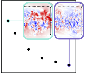
Visualizations of transverse velocity across the mixing layer are shown for the lowest and highest  $M_c$ cases in figure 2. The domains (truncated for visual comparison) are scaled by the total mixing-layer thickness
  $\delta _{99}$ to allow for a direct comparison of eddy length scales. The scale disparity between the two cases is qualitatively obvious; in the next section, the turbulence scales are discussed quantitatively and used to propose an alternative explanation for growth rate reduction.

Figure 2. Instantaneous planar view ( $x$–
$x$– $y$ plane) at
  $z=L_z/2$ slices of transverse velocity
  $v$ at final simulation time for (a)
  $M_c=0.2$ and (b)
  $M_c=2.0$ cases. Arrows indicate decorrelation length scales based on
  $v^\prime$ along
  $x$ and
  $y$ axes.
3. Turbulence length and time scales
In addition to the thickness measures  $\delta _{99}, \delta _\omega$ and
  $\delta _\theta$, which characterize the mean velocity profile, a decorrelation length scale is used to characterize the effect of increasing
  $M_c$ on the energy-containing scales. This length scale,
  $\delta _y$, is defined in (3.1) using a pair of points symmetrically placed around an anchor point
  $y_0$ at a mutual separation distance of
  $\delta _y$. A decrease in the correlation to 0.1 is used to define this length scale, with the anchor point
  $y_0=y_c$ at the shear-layer centre, where
  $\tilde u(y_c)=0$.
 \begin{equation} \frac{\overline{ v'(y_0-\delta_y/2)v'(y_0+\delta_y/2) }}{\overline{v'(y_0)v'(y_0)}} = 0.1. \end{equation}
This length scale as a fraction of total mixing-layer thickness decreases significantly from the quasi-incompressible case at  $M_c=0.2$ to the highly compressible case at
  $M_c=2.0$. Figure 3(a) shows the transverse correlation length for the fluctuating transverse velocity and the effect of shifting the anchor point to
  $y_c\pm \delta _{99}/4$. Present data indicates a threefold decrease (from low to high
  $M_c$) in
  $\delta _y$ along the centreline, and nearly a fourfold decrease in
  $\delta _y$ for points offset from the centreline. Figure 3(a) also indicates that
  $\delta _y$ measured about
  $y_c$ is the minimum decorrelation length in the mixing layer at each
  $M_c$. The occurrence of minimum length scale is intuitive since maximum shear also occurs along the centreline.

Figure 3. Effect of compressibility on (a) normalized decorrelation lengths  $\delta _{y}/\delta _{99}$ for
  $v'$ measured about different
  $y_0$, (b) mean velocity difference
  $U_\delta /{\rm \Delta} \bar {u}$ across the
  $v'$ decorrelation length, and (c) various Mach numbers.
The mean velocity difference across the average decorrelation length scale centred about anchor point  $y_0$, defined as
  $U_\delta$ in (3.2), is also an important turbulent statistic of these eddies. The behaviour of this velocity scale, plotted in 3(b), matches the familiar reduction of normalized growth rates shown in figure 1(b).
 \begin{equation} U_\delta=\tilde{u}\left(y_0+\frac{\delta_y}{2}\right) -\tilde{u}\left(y_0-\frac{\delta_y}{2}\right). \end{equation}
 The time scales of turbulent motions are also inherently linked to the reported decorrelation length scales  $\delta _y$. The most obvious time scale of interest is that of the acoustic scale set by the mean speed of sound
  $\bar {c}=\overline {\sqrt {\gamma p/\rho }}$, which effectively defines the reach of acoustic communication in a mean sense. A second time scale to consider is the one associated with eddy distortion due to the shearing of the mean flow, which corresponds to the centreline (maximum) shear
  $S=\textrm {d}\tilde {u}/{\textrm {d} y}$. Finally, the turbulent time scales associated with the turbulent velocity fluctuations and shear stresses are considered. In this discussion, these time scales are also interpreted as the Mach numbers defined below.
 \begin{equation} M_t = \left.\frac{\sqrt{\widetilde{u_i^{{\prime\prime}}u_i^{{\prime\prime}}}}}{\bar{c}}\right|_{y_c}, \quad M_{t,v} = \left.\frac{\sqrt{\vphantom{\frac{1}{2}}\widetilde{v^{{\prime\prime}}v^{{\prime\prime}}}}}{\bar{c}}\right|_{y_c}, \quad M_{\tau} = \left.\frac{\sqrt{\vphantom{\frac{1}{2}}|\widetilde{u^{{\prime\prime}}v^{{\prime\prime}}}|}}{\bar{c}}\right|_{y_c}, \quad M_g = \left.\frac{S\delta_y}{\bar{c}}\right|_{y_c}. \end{equation}
 The turbulent Mach numbers,  $M_t$, represent the ratio of the mean acoustic time scale to the time scale of turbulent fluctuations. As shown in figure 3(c), while
  $M_t$ shows saturation at the highest
  $M_c$, the turbulent Mach number defined using only the transverse component of TKE,
  $M_{t,v}$, indicates saturation at lower levels of compressibility, as further evidence for the pronounced effect of compressibility on the fluctuating transverse velocity. Freund et al. (Reference Freund, Lele and Moin2000) showed the beginning of a saturated regime for these time scale ratios for an annular mixing layer. The present
  $M_t$ and
  $M_{t,v}$ show this trend at higher
  $M_c$ in a self-similar shear layer. A friction Mach number,
  $M_\tau$, of the turbulent mixing layer can be defined using the turbulent shear stress. In the present simulations,
  $M_\tau \le 0.5$. Even at the lowest
  $M_c$ cases,
  $M_\tau$ remains much larger than the
  $M_\tau$ encountered in turbulent boundary layers of high-speed, compressible flows (Bradshaw Reference Bradshaw1977). As a complement to the
  $M_\tau$ description of turbulent shear, the gradient Mach number,
  $M_g$, describes the compressibility effect of mean shear. The gradient Mach number represents the ratio of the acoustic time scale to the mean deformation time scale. Unlike
  $M_t$, this time scale ratio does not show a clear plateau although such a tendency is suggested by the data. Studies at even higher
  $M_c$ are required to fully demonstrate this saturation.
Even in the most compressible case, each of the Mach numbers investigated in figure 3(c) remain subsonic. The sonic eddy hypothesis, as proposed by Breidenthal (Reference Breidenthal1992), would suggest that since acoustic communication across these eddies is possible, these eddies remain coherent and participate in entrainment. Present data indicates that in the  $M_c$ range of significant growth rate reduction, the energy-containing eddies are subsonic. Assuming that eddies of scale
  $\delta _y$ are active in entrainment, the relative shear across these eddies appears directly related to the growth rate behaviour. At lower
  $M_c$, these eddies span across a large portion of the overall mixing-layer thickness, whereas at high
  $M_c$, the mixing layer consists of several ‘colayers’ of energy-bearing eddies. Figure 4 indicates that several autocorrelation profiles can fit within the mixing-layer thickness at
  $M_c=2.0$, and that this structure is consistently maintained during the self-similar regime. Such behaviour suggests an internal regulation mechanism which limits the formation of still larger scales in the higher
  $M_c$ mixing layers.

Figure 4. Autocorrelation profiles  $R_{22}(y_0)$ for
  $v'$ measured about different
  $y_0$ for (a)
  $M_c=0.2$ and (b)
  $M_c=2.0$ at the beginning (black) and end (blue) of self-similar spreading. Overall mixing-layer thickness
  $\delta _{99}$ is indicated in terms of initial thickness
  $\delta _\theta ^o$.
From figure 3(c), the turbulent Mach number  $M_t$ and transverse turbulent Mach number
  $M_{t,v}$ reach a plateau of approximately 0.5 and 0.2, respectively. The latter suggests that sound has sufficient time to ricochet 2–3 times across the transverse correlation scale during eddy turnover. Motions at still larger scales are evidently unable to remain coherent. They may correspond to acoustic response, but not rotational eddies. Figure 5(a) shows the ratio of correlation scales along
  $x$ and
  $y$ directions,
  $\delta _x/\delta _y$, and along the
  $z$ and
  $y$ directions,
  $\delta _z/\delta _y$ against
  $M_c$ (a data processing error invalidates the corresponding plot in Matsuno & Lele (Reference Matsuno and Lele2020)). Note that these ratios are relatively constant (the
  $M_c=2.0$ point is an outlier since it may be affected by the smaller domain size in
  $x$). The internal regulation mechanism which limits the transverse scale to a decreasing fraction of the total shear-layer thickness
  $\delta _{99}$ also limits the correlation scales in the
  $x$ and
  $z$ directions and maintains approximately the same ratio in correlation scales. All of these trends are consistent with acoustic communication as the regulation mechanism for maintaining coherent eddying motions. Figure 5(b) shows the dimensionless shear number, or Corrsin number,
  $S\delta _y/\sqrt {R_{ii}}=M_g/M_t$ and
  $S\delta _y/\sqrt {R_{22}}=M_g/M_{t,v}$ against
  $M_c, \ {\rm with} \ R_{ii}=\widetilde{u_i^{\prime\prime}u_i^{\prime\prime}} \ {\rm and} \ R_{22}=\widetilde{v^{\prime\prime}v^{\prime\prime}}$. These measures are relatively constant with
  $M_c$, which affirms that the regulation is not associated with an increased importance of shear with
  $M_c$, but with acoustic communication limiting the turbulence length scales in the flow.

Figure 5. (a) Decorrelation ratios and (b) dimensionless shear (Corrsin number).
4. Scaling of Reynolds stress, turbulent production and growth rates
Profiles of Reynolds shear stress magnitudes  $|R_{12}|=|\overline {u^{\prime }v^{\prime }}|$ scaled using the total velocity difference
  ${\rm \Delta} \bar {u}$ and the effective velocity scale
  $U_\delta$ are shown in figure 6. Whereas scaling using
  ${\rm \Delta} \bar {u}$ indicates a steady decline in
  $|R_{12}|$, scaling using
  $U_\delta ^2$ results in a clear separation between Reynolds stress profiles at low versus high
  $M_c$. Turbulent shear stresses scaled by
  ${\rm \Delta} \bar {u}$ reported by Almagro, García-Villalba & Flores (Reference Almagro, García-Villalba and Flores2017) at
  $s=8$ and Baltzer & Livescu (Reference Baltzer and Livescu2020) at
  $s=7$ with
  $M_c\to 0$ are compared to our quasi-incompressible case,
  $M_c=0.2$, in figure 7(c) as confirmation that the variable density stresses are within the range of comparable studies. The scaling for
  $s=7$ cases is similar to that of the
  $s=1$ cases. The internal length scale
  $\delta _y$ and effective velocity scale
  $U_\delta$ in figure 7(a) follow similar declines to those in figures 3(a) and 3(b). Figure 3(b) shows the same scaling in 6(b) applied to
  $|R_{12}|=|\widetilde {u^{{\prime \prime }}v^{{\prime \prime }}}|$ for
  $s=7$ cases. A similar separation arises between the low and high
  $M_c$ cases, and the high
  $M_c$ cases attain scaled magnitudes close to those in the
  $s=1$ cases.

Figure 6. Turbulent shear stress: (a)  $|R_{12}|/({\rm \Delta} \bar {u})^2$; (b)
  $|R_{12}|/U_\delta ^2$; (c) integrated
  $|R_{12}|$ vs.
  $M_c$.

Figure 7. Scaling for  $s=7$ cases: (a) decorrelation scales
  $\delta _y$ and
  $U_\delta$; (b)
  $|R_{12}|/U_\delta ^2$; (c)
  $|R_{12}|/({\rm \Delta} \bar {u})^2$ at
  $M_c=0.2$ compared to recent literature for
  $M_c\to 0$.
Similarly, TKE production and dissipation may be scaled using either the overall mixing-layer scales or the internal scales associated with transverse velocity decorrelation. Figure 8 shows integrated TKE production  $P$, TKE dissipation
  $D$, and pressure-strain component
  $\varPi _{11}=2\overline {p^\prime (\textrm {d} u^{{\prime \prime }}/{\textrm {d} x})}$, which acts to transfer energy out of
  $R_{11} = \widetilde{u^{\prime\prime}u^{\prime\prime}}$, scaled by
  $\delta _{99}/({\rm \Delta} \bar {u})^3$ and
  $\delta _y/U_\delta ^3$. The production term is related to the growth rate definition offered by Vreman et al. (Reference Vreman, Sandham and Luo1996), such that the values plotted in figure 8(a) represent
  $\dot {\delta }_{\theta }\times \rho _\infty \delta _{99}/(2\delta _\theta {\rm \Delta} \bar {u})$. Dissipation normalized with internal scales transforms the trend of progressive decrease of the quantity with
  $M_c$ to an approximately constant value for
  $M_c>0.2$. Internally scaled production and pressure-strain
  $\varPi _{11}$ show a similar asymptotic behaviour past
  $M_c\sim 0.8$. The asymptotic approach towards constant production, pressure-strain and dissipation, as well as evidence for constant turbulent shear stress magnitudes using the effective velocity scale
  $U_\delta$ further suggests the importance of
  $\delta _y$ as the defining length scale associated with turbulent mixing. This distinction may improve length-scale-based turbulence models.

Figure 8. Selected TKE budget terms, integrated and scaled with (a) total thickness  $\delta _{99}$ and total velocity difference
  ${\rm \Delta} \bar {u}$ and with (b) internal scales
  $\delta _y$ and
  $U_\delta$.
5. Conclusion
In this work, the scales governing the turbulent structures in mixing layers with notable compressibility and density effects are thoroughly characterized. It is confirmed that as  $M_c$ increases, turbulence length scales, including the transverse length scale, reduce dramatically as a fraction of the overall shear-layer thickness. These length scales appear to be limited by acoustic communication; turbulence-associated Mach number(s) show saturation at higher levels of compressibility. The internal regulation adapts the spatial and temporal scales of shear-layer turbulence inferred from two-point correlations. It reduces the effective velocity scale, suppresses pressure fluctuations and mixing-layer growth rate. To accurately capture the effects of compressibility in free shear flows, turbulence models should capture not only the increasing anisotropy of turbulent stresses, but also the reduction in the turbulence length scales.
Acknowledgements
Simulations are supported by US Department of Energy Office of Science INCITE allocation 4978-4846 and through Argonne Leadership Computing Facility Director's Discretionary allocation 6195-6063. K.M. is funded by the NSF GRFP (National Science Foundation Graduate Research Fellowship Program). S.K.L. acknowledges partial support from NSF CBET 1803378.
Declaration of interests
The authors report no conflict of interest.


