2. Eulerian vs Lagrangian perspectives

Consider the standard distinction between the Eulerian and Lagrangian perspectives on fluid flow inside a fixed manifold $S$ . In the Eulerian perspective, we imagine standing still at a fixed point in $S$ and watching the fluid flow past us. The Eulerian specification of the flow field at a point $p \in S$ and at time $t$ is therefore a vector $\textbf{v}_t(p)$ in the tangent space $\text {T}_p S$ to the point $p$ that gives the direction in which matter is flowing past us. Globally, this results in a time-dependent vector field $\textbf{v}_t$ on $S$ , a path in the space $\mathfrak {X}(S)$ of vector fields on $S$ . By contrast, the Lagrangian perspective instead considers the medium to be made up of fluid particles, whose paths we follow through time. At time $t$ , the fluid particle that was initially at point $p \in S$ has moved to some new point $\psi _t(p) \in S$ . For a smooth fluid motion, this gives rise to a time-dependent diffeomorphism $\psi _t$ of $S$ , a path in the diffeomorphism group $\text {Diff}(S)$ –recall that a diffeomorphism is nothing more than a smooth and invertible relabelling of the points of $S$ , and that two diffeomorphisms can be composed to give another diffeomorphism, which gives the collection $\text {Diff}(S)$ of all diffeomorphisms the mathematical structure of a group. Crucially, these two perspectives are completely equivalent and can be mapped onto one another: the Eulerian flow field $\textbf{v}_t$ and the Lagrangian diffeomorphism $\psi _t$ are related by

(2.1) \begin{equation} \textbf{v}_t \circ \psi _t = \partial _t \psi _t, \end{equation}

where $\partial _t$ denotes partial differentiation with respect to time.

The deeper mathematical relationship between Eulerian and Lagrangian perspectives has been studied using the language of differential geometry and Lie group theory, a set of ideas originally developed by Arnold (Reference Arnold2014) and described in detail in the textbook of Arnold & Khesin (Reference Arnold and Khesin2021). We will not give a detailed discussion of this theory here, and instead only concern ourselves with aspects salient to the differences between ordinary fluid dynamics and the motion of deformable surfaces. Chief amongst these is the use of (2.1) to interpret $\partial _t \psi _t$ as a vector field on $S$ : while this is fine in the setting of ordinary fluid dynamics, trying to carry this reasoning over to the setting of deformable surfaces requires care.

Properly, a Lagrangian motion is a path through the diffeomorphism group $\text {Diff}(S)$ (or the group $\text {SDiff}(S)$ of volume-preserving diffeomorphisms for an incompressible flow). At each time $t$ the tangent direction $\partial _t \psi _t$ to this path lies in the tangent space $\text {T}_{\psi _t} \text {Diff}(S)$ to the diffeomorphism group at the point $\psi _t$ . At any point the tangent space to the diffeomorphism group can be identified with its Lie algebra, and this is nothing more than the space $\mathfrak {X}(S)$ of vector fields on $S$ – thus, for any fixed $t$ , $\partial _t \psi _t$ can be understood as a vector field on $S$ . When considering the motion and deformation of fluid surfaces, however, this identification is more complicated, and correspondingly the relationship between the Eulerian and Lagrangian perspectives is more complicated.

Notably, when dealing with deformable surfaces there is not one manifold, but three: an abstract body $B$ , which in our case is a two-dimensional (2-D) manifold because we are considering a deformable surface; an ambient space in which the motion happens, which for us will always be 3-D Euclidean space $\mathbb {R}^3$ equipped with the Euclidean metric $e$ ; and the image $M$ of $B$ in $\mathbb {R}^3$ , which is the physical surface which we observe. The ambient space is the natural analogue of the fixed manifold in ordinary fluid dynamics, and must remain invariant under any dynamics. The body is not usually equipped with a metric, but often has a volume form $\mu$ which is interpreted as a density measure for an unstrained configuration, and is necessary to describe conservation of mass and incompressibility.

To clarify, we consider a configuration of the system as an embedding $r : B \to \mathbb {R}^3$ of the body into the ambient space, whose image is the material, a smooth submanifold $M$ of $\mathbb {R}^3$ . The collection of all such embeddings is a space $\text {Emb}$ which has the structure of an infinite-dimensional manifold – the details of infinite-dimensional spaces are not relevant to our discussion here, what is relevant is that intuitive notions of smooth paths and variations make sense in this context. A motion of the system is then a path $r_t : B \to \mathbb {R}^3$ of embeddings with images $M_t$ , that is, a path in $\text {Emb}$ – the role played by this space is therefore analogous to the role played by the diffeomorphism group $\text {Diff}(S)$ in the case of ordinary fluid dynamics in a fixed space $S$ .

The derivative $\partial _t r_t$ defines a tangent vector to this path in the space $\text {Emb}$ . Define $\textbf{U}_t$ to be the value of this derivative at time $t$ , an element of $\text {T}_{r_t}\text {Emb}$ : this is a map $\textbf{U}_t : B \to \text {T}\mathbb {R}^3$ . For a deformable surface this map is the analogue of the derivative $\partial _t \psi _t$ of the diffeomorphism giving the Lagrangian description of the motion. However, note that this map is not a vector field, either on $B$ or in $\mathbb {R}^3$ , and it cannot be identified with one via the relationship (2.1) used in ordinary fluid dynamics because the tangent space to $\text {Emb}$ is not isomorphic to a space of vector fields. This is one of the key differences when considering the motion of a deformable surface.

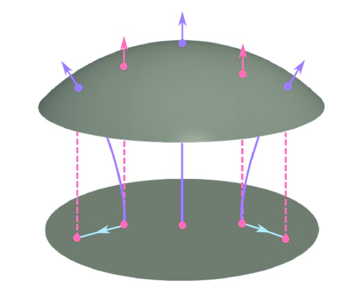
Figure 1. An embedding $r_t$ of an abstract space $B$ into $\mathbb {R}^3$ induces a vector field $\textbf{V}_t$ on $B$ called the left Eulerian velocity, as well as a map $\textbf{v}_t : M_t \to \text {T}\mathbb {R}^3$ on the image $M_t$ of the embedding. We interpret that latter as a vector field along $M_t$ which has a part tangent to $M_t$ but may also have a part normal to $M_t$ , and refer to it as the right Eulerian velocity. Pulling back this vector field along the embedding $r_t$ ‘forgets’ the normal part, yielding the left Eulerian velocity $\textbf{V}_t$ . The mathematical relationships between these maps are shown in the diagram on the left, while a more visual representation is shown on the right. Here, $\text {T}r_t$ denotes the tangent map (matrix of partial derivatives) induced by $r_t$ , $\pi$ is the projection from the tangent bundle to the underlying manifold and $\textbf{U}_t = \partial _t r_t$ as described in the text.

We can derive two vector fields from the map $\textbf{U}_t$ according to the diagram shown in figure 1. The first of the two vector fields is the “right Eulerian velocity”, a map $\textbf{v}_t : M_t \to \text {T}\mathbb {R}^3$ defined by

(2.2) \begin{equation} \textbf{v}_t := \textbf{U}_t \circ r^{-1}_t. \end{equation}

This is a vector field in $\mathbb {R}^3$ defined along $M_t$ . As such, it decomposes as $\textbf{v}_t = \textbf{v}^\parallel _t + v^n_t\textbf{n}_t$ , where $\textbf{v}^\parallel _t$ is tangent to $M_t$ and $\textbf{n}_t$ is the normal. There is also the ‘left Eulerian velocity’, a vector field $\textbf{V}_t : B \to \text {T}B$ on $B$ defined by

(2.3) \begin{equation} \textbf{V}_t := (\text {T}r_t)^{-1} \circ \textbf{U}_t. \end{equation}

Here, $\text {T}r_t$ denotes the tangent map induced by the embedding; see Appendix C for the definition. The right Eulerian velocity pulls back to the left Eulerian velocity, $r^*_t \textbf{v}_t = \textbf{V}_t$ , but for purely dimensional reasons the normal component is lost and the pushforward of the left Eulerian velocity is accordingly $r_{t*} \textbf{V}_t = \textbf{v}^\parallel _t$ , the tangent part $\textbf{v}_t$ .

Neither of these vector fields quite corresponds to our intuitive idea of Eulerian motion: the right Eulerian velocity $\textbf{v}_t$ is defined on a surface that is intrinsically moving; the left Eulerian velocity does not encode the normal motion of the surface. To properly specify the Eulerian and Lagrangian descriptions of surface motion, we need to introduce a small amount of additional structure which formally captures some intuitive notions about surface dynamics that would be unnecessary if $B$ were itself a 3-D body.

The manifold $M_t$ has two natural vector bundles associated with it. The first is $\text {T}M_t$ , its usual 2-D tangent space. However, we also need to consider directions that contain a component normal to $M_t$ , and these lie in a 3-D bundle that we denote by $E_t$ , the restriction of $\text {T}\mathbb {R}^3$ to $M_t$ . The Euclidean metric defines an orthogonal splitting $E_t = \text {T}M_t \oplus N_t$ , where $N_t$ is the 1-D normal bundle. The orthogonal projection of the Euclidean metric onto $\text {T}M_t$ is then exactly the induced metric on $M_t$ (the first fundamental form). The right Eulerian velocity $\textbf{v}_t$ is a section of the bundle $E_t$ ; to be explicit, a vector field defined along $M_t$ that has both tangent and normal components. This bundle is visualised in figure 2.

We fix an initial embedding $r_0$ with image $M_0$ . The motion $r_t$ then induces diffeomorphisms $\lambda _t : M_0 \to M_t$ with $\lambda _t = r_t \circ r^{-1}_0$ . The path $\lambda _t(p)$ of some point $p \in M_0$ is then naturally seen as the motion of a fluid particle in the ambient space $\mathbb {R}^3$ , as thus is the a Lagrangian description of the motion. We have the relationship

(2.4) \begin{equation} \textbf{v}_t \circ \lambda _t = \partial _t \lambda _t, \end{equation}

and hence the right Eulerian velocity $\textbf{v}_t$ is the vector field naturally associated with the Lagrangian motion $\lambda _t$ .

The Eulerian description must involve standing at a fixed point on the initial manifold $M_0$ . If $M_t$ were a 3-D manifold, there we would be no problem with pulling back the velocity field $\textbf{v}_t$ on $M_t$ along $\lambda _t$ to give a vector field on $M_0$ that naturally corresponds to the Eulerian picture of the motion Casey & Papadopoulos (Reference Casey and Papadopoulos2002). Because we consider a 2-D surface this does not work out for dimensional reasons, but this is a purely technical issue that can easily be resolved with a simple definition.

Figure 2. Comparison of the Eulerian and Lagrangian pictures for motion in a fixed surface (a) and for a deformable surface (b). In a fixed plane $\mathbb {R}^2$ , the Lagrangian picture involves a diffeomorphism $\psi _t$ of $\mathbb {R}^2$ that moves a fluid particle initially the point $p$ to the point $\psi _t(p)$ . We may also consider an Eulerian picture, where we stand still at the point $p$ and watch the fluid flow past us, its direction at time $t$ being given by the vector $\textbf{v}_t(p)$ . A deformable surface $M_t$ embedded in $\mathbb {R}^3$ undergoes a Lagrangian motion described by a diffeomorphism $\lambda _t : M_0 \to M_t$ that maps the initial surface onto the time $t$ surface. The associated right Eulerian velocity field $\textbf{v}_t$ lies in the extended tangent space $E_t$ to $M_t$ , as described in the text. By pulling back the entire tangent space via $\lambda _t$ (inset) as described in the text we can define a time-varying vector field $\textbf{s}_t$ along $M_0$ which plays the role of the Eulerian velocity at a fixed point $p \in M_0$ .

The map $\text {T}\lambda _t : \text {T} M_0 \to \text {T} M_t$ associates a tangent vector on $M_0$ with a tangent vector on $M_t$ . Let us define a map $A_t : E_0 \to E_t$ that acts on the spaces of 3-D vector fields along $M_0$ and associates them with 3-D vector fields along $M_t$ . To define this map, we use the splitting $E_t = \text {T}M_t \oplus N_t$ into a tangent space and a normal bundle. By linearity, it suffices for us to define that $A_t$ acts on the $\text {T}M_0$ factor exactly as $\text {T}\lambda _t$ , and acts on the $N_0$ factor by mapping the unit normal $\textbf{n}_0$ to $M_0$ to the unit normal $\textbf{n}_t$ to $M_t$ . Now, we may naturally define a section $\textbf{s}_t$ of $E_0$ by

(2.5) \begin{equation} \textbf{s}_t(p) := A_t^{-1} \circ \textbf{v}_t \circ \lambda _t(p). \end{equation}

Concretely, if $\textbf{v}_t \circ \lambda _t = \textbf{v}^\parallel _t + v^n_t \textbf{n}_t$ , then

(2.6) \begin{equation} \textbf{s}_t(p) = \lambda ^*_t\textbf{v}^\parallel _t + (\lambda _t^* v^n_t)\textbf{n}_0. \end{equation}

Then $\textbf{s}_t$ is always a 3-D vector field along $M_0$ , as we may consider it to be the Eulerian flow field of the motion. It of course satisfies $\textbf{s}_0 = \textbf{v}_0$ , because the map $A_0$ is just the identity map. We visualise this pullback process in figure 2. We could also describe this in a convective representation on the manifold $B$ , by pulling the whole bundle $E_t$ back along the embedding $r_t$ , and taking the pullback $r^*_t \textbf{s}_t$ as the left Eulerian velocity, a section of $r^*_t E_t$ .

The ways in which the terms ‘Eulerian’ and ‘Lagrangian’ are often used in the literature – especially in computational studies (Torres-Sánchez et al. Reference Torres-Sánchez, Millán and Arroyo2019, Reference Torres-Sánchez, Santos-Oliván and Arroyo2020; Sahu et al. Reference Sahu, Omar, Sauer and Mandadapu2020b ) – refers to something quite different from the Eulerian–Lagrangian split we have just outlined. Rather, they describe different ways of parameterising quantities on the surface in terms of a surface frame field: this may be convected with the fluid (‘Lagrangian’) or not (‘Eulerian’). The freedom to choose the frame is a kind of ‘gauge freedom’, and the physics is agnostic to the particular choice of gauge. There are, in fact, several gauge freedoms that arise in the mathematical formulation of morphodynamics, some of which leave the physics invariant and some of which do not, and these choices play an essential role in the formulation of objectivity and observer motion. We describe this in detail in the next section.

3. Gauge freedom

We describe gauge freedoms in the usual language of gauge theory in physics, in terms of the action of a symmetry group and the principal bundle which it defines (Frankel Reference Frankel2011; Naber Reference Naber2011 Reference Naber a ,Reference Naber b ). We introduce this technical language to help make contact with other areas of physics and also for precision, but a familiarity with it is not essential to follow the key arguments of this section, as long as the reader grasps the intuitive notion of a symmetry group acting on a space, which we describe now.

Informally, a group action describes the way that transformations move points around in a physical space. For example, the circle group acts on a plane by rotations: the rotation by an angle $\alpha$ maps a point specified by $(r, \theta )$ in polar coordinates to the point $(r,\theta +\alpha )$ . The group act divides the space up into pieces that it leaves invariant –in our example, these pieces are circles of constant radius in the plane, since any rotation will keep the points on one of these circles on that circle. This partition of the space up into a parameterised family of pieces is, loosely, the concept of a bundle.

In order to help fix ideas, we briefly comment on how gauge freedoms manifest in the motion of a fluid in a fixed space $S$ . There is a natural action of the group $\text {Diff}(S)$ on this space which captures the notion of a Lagrangian flow – a diffeomorphism $\psi$ moves the point $p$ to the point $\psi (p)$ in $S$ . It has a subgroup $\text {Isom}(S)$ of isometries, those diffeomorphisms $\phi$ that fix the metric $g$ on $S$ , $\phi ^* g = g$ . In $n$ -dimensional Euclidean space this is the Euclidean group $\text {E}(n)$ of rotations and translations. If we add in time-dependent isometries with a constant velocity, so-called Galilean boosts, then we obtain the Galilean group, $\text {Gal}$ . Hydrodynamics is manifestly not invariant under the action of $\text {Diff}(S)$ , but it is required to be invariant under $\text {Gal}$ . This then corresponds to a gauge freedom in how we specify our equations of motion, as we are free to describe the physics itself in any inertial reference frame. Informally, objectivity is the invariance of our equations of motion under the action of the Galilean group, which can be interpreted as their invariance under a motion of a hypothetical observer in an inertial reference frame.

There is a second gauge freedom which is not concerned with the physics, but simply the representation of physical quantities. A frame field on $S$ is a choice of basis for the tangent space $\text {T}_p S$ at every point $p$ , which varies smoothly on space. We should be careful to disambiguate this from the notion of an inertial reference frame or a hypothetical observer, and hence from the notion of objectivity – it is a fundamentally different concept. To describe a physical quantity that is a vector or a tensor – for example the velocity field $\textbf{v}$ – we pick some frame field $\textbf{e}_j$ – for example a coordinate frame – which spans the tangent space to $S$ , and then we may write $\textbf{v} = v^j\textbf{e}_j$ for some set of functions $v^j$ . However, the frame field is entirely arbitrary and bears no relation to the physics. We are free to choose a different frame field $\bar {\textbf{e}}_j$ and instead write $\textbf{v} = \bar {v}^j\bar {\textbf{e}}_j$ . Of course, the vector field $\textbf{v}$ does not change under a change of frame, and it does not matter whether the frame field is a coordinate frame, whether it is orthonormal, or whether it varies in time. This freedom to choose the frame field is then associated with the action of $\text {Diff}(S)$ not on the manifold itself, but on the frame bundle $\text {F}S \to S$ , an action which sends a frame $\textbf{e}_j$ to the new frame $\psi _*\textbf{e}_j$ .

Now we return to the setting of deformable surfaces. In this problem there are really three distinct gauge freedoms, and part of the confusion around objectivity and “Eulerian” vs “Lagrangian” motions has to do with a failure to properly disambiguate between them. The state of the deforming surface is captured by an element $r \in \text {Emb}$ . There are two group actions on this space: $\text {E}(3)$ and $\text {Diff}(B)$ act on $\text {Emb}$ respectively from the right and the left.

The first group $\text {E}(3)$ is the isometry group of the ambient space, and it reflects our ability to change reference frames in the ambient space (not on the surface). The second group $\text {Diff}(B)$ is the diffeomorphism group of $B$ , and its action on $\text {Emb}$ reflects our ability to make arbitrary changes of coordinate system in the base space. This is a gauge freedom related to the parameterisation of the motion of the surface itself, independently on any physics or quantities defined on the surface. The third gauge freedom again concerns an action of $\text {Diff}(B)$ , but this time on the frame bundle $\text {F}B \to B$ ; equivalently, an action of the diffeomorphism group $\text {Diff}(M_t)$ of the embedded surface at time $t$ on its own frame bundle $\text {F}M_t \to M_t$ . Informally, a frame on $M$ consists of a choice, for each point $p \in M$ , of basis for the tangent space $T_pM$ , and the frame bundle $FM \to M$ consists of all possible choices of frame on $M$ – for example, any global choice of coordinate function defines a frame. As with motion in a fixed space, this group action describes our freedom in choosing a local frame field with which to represent quantities defined along the surface.

We concretely define each of these group actions and their associated gauge freedoms in the following subsections, and describe their physical interpretation in more detail.

3.1. Gauge freedom in the ambient space

First we describe the action of the isometry group. For an isometry $\phi \in \text {E}(3)$ and embedding $r \in \text {Emb}$ , the group action sends $r$ to the composition $\phi \circ r$ and sends the image $M$ of $r$ to a different submanifold $\phi (M)$ . While these two submanifolds will in general be different, they are related by a rigid body motion and not by a deformation (that is, a “pure motion”) and the first and second fundamental forms induced on $\phi (M)$ are the same as those on $M$ – more precisely, the pullbacks of these quantities to $B$ are equal.

Readers familiar with bundle theory may appreciate an alternative perspective on this: it is possible to view this gauge freedom as introducing a fibre bundle structure on $\text {Emb}$ , parameterising the choices of “observer reference frame” in the ambient space in the following way. Group actions on a space define quotient spaces and principal bundles over those spaces (Frankel Reference Frankel2011; Naber Reference Naber2011 Reference Naber a ,Reference Naber b ), by collapsing any submanifold left invariant by the group action down to a single point in the quotient. We define $\text {Iso}$ to be the quotient space defined by the action of $\text {E}(3)$ on $\text {Emb}$ . This is the space of deformable surfaces up to isometry, which can be interpreted as surfaces with a fixed centre of mass (we can always use a translation to move this to the origin) and a fixed orientation at the centre of mass (a global rotation ensures this can always point along the $z$ -axis). Alternatively, we may view it as the space of deformable surfaces with a single fixed point $p$ at which the normal direction never changes. Associated with $\text {Iso}$ is the fibre bundle

(3.1) \begin{equation} \text {E}(3) \to \text {Emb} \to \text {Iso}. \end{equation}

Sitting above a point in $\text {Iso}$ is the group $\text {E}(3)$ which parameterises all possible placements and orientations for the centre of mass (equivalently a fixed point $p$ ) of the surface – this is the gauge freedom, and fixing a given isometry returns us to a point in the full space $\text {Emb}$ . A path of distinct embeddings which correspond to the same point in $\text {Iso}$ can be distinguished by an observer stood at a fixed point in space, but if the observer is allowed to move with the surface they can change their position so that their view of it never changes. More succinctly, in $\text {Iso}$ we see only deformation and not the motion.

The action of $E(3)$ is then associated with a gauge freedom – the equations of motion are invariant under the action of $E(3)$ , and so the physics does not really “see” motion in $\text {Emb}$ , it only sees motion in the quotient space $\text {Iso}$ .

As we saw in the case of a fixed space, the definition of objectivity requires extending this group action to the larger space of time-dependent isometries, of which the Galilean group $\textit{Gal}$ is a subgroup. We discuss this, including some of the subtleties, in more detail in the next section.

3.2. Gauge freedom on the deforming surface

The group $\text {Diff}(B)$ acts on $\text {Emb}$ as follows. Let $r \in \text {Emb}$ be an embedding and $\psi$ a diffeomorphism (coordinate change) of $B$ . The action of $\text {Diff}(B)$ sends $r$ to $r \circ \psi$ . The image of $B$ under $r \circ \psi$ is the same as its image under $r$ , i.e. these two different embeddings define exactly the same submanifold $M$ of $\mathbb {R}^3$ , but they correspond to distinct points in $\text {Emb}$ . This coordinate change therefore induces no motion and no deformation of the surface. Instead of considering motion relative to $B$ we may instead consider it relative to $M_0$ , the initial material surface, in which case we consider the action of the group $\text {Diff}(M_0)$ – clearly isomorphic to the group $\text {Diff}(B)$ – acting to change coordinates in the initial surface, with corresponding action on the diffeomorphism $\lambda _t: M_0 \to M_t$ .

Again, it may help readers familiar with bundle theory to view this gauge freedom as parameterising choices of coordinates on the surface via a fibre bundle structure on $\text {Emb}$ . The quotient space defined by the action of $\text {Diff}(B)$ on $\text {Emb}$ is the ‘space of membranes’ $\text {Memb}$ , which can alternatively be described as the collection of all images of embeddings

(3.2) \begin{equation} \text {Memb} = \{r(B) \ | \ r \in \text {Emb} \}. \end{equation}

From the perspective of an outside observer it is impossible to distinguish points in $\text {Emb}$ that correspond to the same point of $\text {Memb}$ , even if the observer moves around – all that distinguishes them is the patameterisation of the surface, which has no physical meaning. We then have an associated fibre bundle,

(3.3) \begin{equation} \text {Diff}(B) \to \text {Emb} \to \text {Memb}. \end{equation}

Sitting above each point in $\text {Memb}$ – which is nothing more than some submanifold $M$ of Euclidean space with the same topology as $B$ – is a copy of the group $\text {Diff}(B)$ , which can be thought of as parameterising all possible coordinate systems on $M$ .

We want to consider the effects of changing this particular gauge on our description of the motion. Let $r_t : B \to \mathbb {R}^3$ be any path of embeddings describing a motion, with image $M_t$ , and let $\psi _t$ be an arbitrary time-dependent diffeomorphism of $B$ . We associate with $\psi _t$ its “drive velocity” $\textbf{w}^\psi _t = (\partial _t \psi _t) \circ \psi ^{-1}_t$ , which is a vector field on $B$ which can be seen as the velocity of an observer moving around on $B$ (not in the ambient space) starting at an initial point $p$ whose own (Lagrangian) motion is $\psi _t(p)$ . A time-dependent drive velocity generates a “fictitious flow” $\partial _t \textbf{w}^\psi _t$ on the surface, and thus the hydrodynamics of any physical quantity defined on the surface is not invariant under this group action even though the motion of the surface itself is.

Concretely, if we define a new embedding $r^\psi _t := r_t \circ \psi _t$ , then this embedding has the same image $M_t$ as $r_t$ and the associated right Eulerian velocity field is

(3.4) \begin{equation} \textbf{v}_t^\psi = \textbf{v}_t + r_{t*}\textbf{w}^\psi _t, \end{equation}

where $\textbf{v}_t = (\partial _t r_t) \circ r^{-1}_t$ is the Eulerian velocity field associated with $r_t$ . We note that, since $\textbf{w}^\psi _t$ is a vector field on $B$ , its pushforward $r_{t*}\textbf{w}^\psi _t$ is a tangent vector field on $M_t$ with no component along the normal direction. In particular, this suggests a natural choice of gauge transformation in which $\psi _t$ is chosen so that $-r_{t*}\textbf{w}^\psi _t$ is exactly the tangential part of $\textbf{v}_t$ , and hence the velocity field in this gauge is directed along the normal direction to $M_t$ . Indeed, this gauge can be defined as one in which the pullback of $\textbf{v}_t^\psi$ vanishes, which obviously requires that

(3.5) \begin{equation} 0 = r^*_t \textbf{v}_t^\psi = \textbf{V}_t + \textbf{w}^\psi _t. \end{equation}

We call this the ‘normal gauge’. This tells us that the space $\text {Memb}$ only ‘sees’ the normal part of the motion and never the tangential part, which can always be cancelled out by a relabelling of the fluid particles. Computationally, when describing the evolution of the deforming surface itself (but not quantities on the surface) it is convenient to work in the space $\text {Memb}$ , moving the mesh points purely along the normal direction Torres-Sánchez et al. (Reference Torres-Sánchez, Millán and Arroyo2019). Because the surface is invariant under these gauge transformations this presents no issue. However, $\text {Memb}$ ignores all evolution on the surface, and therefore we cannot describe the evolution of other quantities on the surface in this gauge, only the motion of the surface itself.

Figure 3. (a) Construction of a Monge gauge. The evolution of an initially flat surface (green) can be decomposed as a pair $(\psi _t(p), h_t(p))$ where $\psi _t$ (orange) is a diffeomorphism is the initial surface $M_0$ and the $h_t$ is a height function. By making a time-dependent change of gauge using the inverse $\psi ^{-1}_t$ as described in the text, we can ensure the evolution is determined purely by a gauge-transformed height function $h_t \circ \psi ^{-1}_t$ , which ensures a fluid particle initially at the point $p$ evolves purely in the vertical direction (pink). (b) Transition from the Monge gauge (pink) to the normal gauge (purple). This involves a diffeomorphism $\psi _t^N$ (blue) whose drive velocity is $-\nabla h^M_t$ , where $h^M_t = h_t \circ \psi _t^{-1}$ is the height function in the Monge gauge. In the Monge gauge the velocity vector of the surface is $\textbf{v}^M = v^M \textbf{e}_z$ , while in the normal gauge it is $\textbf{v}^N = v^N (\textbf{e}_z -\nabla h^M)$ .

For a concrete example of this gauge transformation, choose $B = \mathbb {R}^2$ to be a plane. Let us fix the usual $x,y,z$ on $\mathbb {R}^3$ , and identify $B$ with the plane $M_0$ with coordinates $(x,y,0)$ . Thus the deforming surface $M_t$ at time $t$ can be related to its initial value by the Lagrangian motion $\lambda _t$ , which can be written in the form

(3.6) \begin{equation} \lambda _t(x, y) = (\psi _t(x, y), h_t(x, y)). \end{equation}

In this expression $\psi _t : \mathbb {R}^2\to \mathbb {R}^2$ is a diffeomorphism of $M_0$ and $h_t : \mathbb {R}^2 \to \mathbb {R}$ is a ‘height’ function. At a point $p = (x,y,z)$ that lies on $M_t$ the velocity field is

(3.7) \begin{equation} \textbf{v}_t(p) = (\partial _t \psi _t) \circ \psi _t^{-1}(x,y) + h_t(\psi ^{-1}_t(x,y))\textbf{e}_z, \end{equation}

where $\textbf{e}_z$ is the unit vector along the Cartesian $z$ direction in $\mathbb {R}^3$ . Now we make a change of gauge using the diffeomorphism $\psi _t^{-1} \in \text {Diff}(M_0)$ . The Lagrangian motion in this new gauge is $\lambda ^M_t = \lambda _t \circ \psi _t^{-1}$ , or in coordinates

(3.8) \begin{equation} \lambda ^M_t(x, y) = (x, y, h_t(\psi _t^{-1}(x, y))). \end{equation}

Defining $h^M_t = h_t \circ \psi _t^{-1}$ , we see that that the motion in this gauge can be described entirely in terms of a height function. We call this the ‘Monge gauge’ (Monge Reference Monge1850) because it is related to a local parameterisation of the surface in terms of Monge patches, and we illustrate this transition in the leftmost panel of figure 3 a.

It is easy to see the transformation from the Monge gauge to the normal gauge. The normal direction on the surface is $\textbf{e}_z - \nabla h_t^M$ , and so we see that the transformation to this gauge involves a diffeomorphism $\psi ^N_t \in \text {Diff}(M_0)$ with drive velocity $\textbf{w}^N_t = -\nabla h_t^M$ . This describes the motion of a surface in the quotient space $\text {Memb}$ , where the velocity is only ever in the normal direction. This is illustrated in the rightmost panel of figure 3 b.

3.3. Frame fields

To express vector and tensor quantities on the deforming surface $M_t$ we choose a frame field $\textbf{e}_1, \textbf{e}_2, \textbf{n}$ spanning the bundle $E_t$ along $M_t$ where $\textbf{n}$ is the unit normal and $\textbf{e}_j$ is a tangential frame field on $M_t$ – that is, for each point $p \in M_t$ we choose a basis for $E_t$ at $p$ , such that this basis varies smoothly as we move around on $M$ . Given that our deformable surface is moving in time, our frame will also vary in time. The most natural way to define the tangential frame is to pick a fixed set of coordinates $x_1, x_2$ on the base space $B$ and push the coordinate directions $\textbf{e}_{x_j}$ , $j=1,2$ , forwards along the embedding $r_t$ to give a frame for the tangent space to $M_t$

(3.9) \begin{equation} \textbf{e}_j := r_{t*} \textbf{e}_{x_j}. \end{equation}

Conversely, any tangential frame field specified on $M_t$ can be pulled back to give a frame field on $B$ . The gauge freedom is then associated with the freedom to pass to a different frame field on $B$ (or equivalently $M_t$ ).

A frame field obtained by pushing forward a constant coordinate basis is what Torres-Sánchez et al. (Reference Torres-Sánchez, Millán and Arroyo2019) refer to as a “Lagrangian parameterisation”. This is because the frame freely moves along with the flow field, and therefore it is conceptually “Lagrangian”, although we emphasise that it has nothing to do with the Eulerian–Lagrangian split in the formulation of hydrodynamics we outlined in § 2. The tangent part of this frame field is advected along with the velocity field of the surface according to

(3.10) \begin{equation} \partial _t \textbf{e}_j = -L_{\textbf{v}} \textbf{e}_j. \end{equation}

We are of course free to choose a different time-dependent frame $\bar {\textbf{e}}_j(t)$ on $B$ (which may or may not be associated with time-dependent coordinates $x_j(t)$ ) and push it forward to give a frame $\textbf{e}_j := r_{t*} \bar {\textbf{e}}_j$ on the surface. The choice is completely arbitrary; this is what Torres-Sánchez et al. (Reference Torres-Sánchez, Millán and Arroyo2019) and Sahu et al. (Reference Sahu, Omar, Sauer and Mandadapu2020b ) refer to as an ‘arbitrary mixed Eulerian–Lagrangian parameterisation’. The time evolution is then

(3.11) \begin{equation} \partial _t \textbf{e}_j = -L_{\textbf{v}} \textbf{e}_j + r_{t*} \partial _t \bar {\textbf{e}}_j. \end{equation}

There is a special case where the frame on $B$ is chosen so that $r_{t*}\partial _t \bar {\textbf{e}}_j = -\nabla _i v^j \textbf{e}_j$ ; that is, the frame field is not advected by the tangential part of the flow. This is the standard choice for hydrodynamics in a fixed space. For a deforming surface, this gives rise to the concept of a frame that is advected only by the normal part of the flow, which conceptually corresponds to an observer that is ‘standing still’ on the deforming surface. Torres-Sánchez et al. (Reference Torres-Sánchez, Millán and Arroyo2019) refer to this as an ‘Eulerian parameterisation’.

In the language of group actions, this freedom to choose the tangential part of the frame field is associated with the action of $\text {Diff}(B)$ on the frame bundle $\text {F}B \to B$ , where the diffeomorphism $\psi \in \text {Diff}(B)$ acts on a frame by pushforward. Because our surface is evolving in time we consider time-dependent paths of frame fields defined by the pushforward along a time-dependent diffomorphism $\psi _t$ . The gauge transformations associated with parameterisations of the surface in the “Monge gauge” and “normal gauge” that we introduced in the previous subsection act on the frame bundle $\text {F}B$ , selecting a frame field that moves only in the $z$ direction and only in the normal direction respectively; the latter is of course the “Eulerian parameterisation” of Torres-Sánchez et al. (Reference Torres-Sánchez, Millán and Arroyo2019). An arbitrary time-dependent change of gauge then gives a “mixed Eulerian–Lagrangian parameterisation” (Torres-Sánchez et al. Reference Torres-Sánchez, Millán and Arroyo2019; Sahu et al. Reference Sahu, Omar, Sauer and Mandadapu2020b ), of which the Monge gauge is a particular example.

4. Objective rates

We now consider questions of objectivity and objective rates in fluid dynamics. Physical quantities are not generally required to be invariant under general diffeomorphisms, as a change to a non-inertial reference frame will introduce ‘fictitious forces’ as we described in the previous section – a familiar example is the Coriolis force experienced by a rotating observer. However, proper formulation of physical laws requires them to be invariant under an appropriate subgroup of symmetry transformations, represented by diffeomorphisms, which gives rise to the concept of objectivity. Which group of transformations is required by objectivity is determined by the physics of the object under consideration.

For hydrodynamics in a fixed space $S$ , a rate $D_{\textbf{v}_t}$ is a way of taking the derivative of material quantities along the Eulerian flow field $\textbf{v}_t$ . To be a rate, the map $D$ must satisfy the Liebniz rule: for any time-dependent tensor field ${\boldsymbol {\sigma }}_t$ and function $f_t$ of time

(4.1) \begin{equation} D(f_t{\boldsymbol {\sigma }}_t) = (Df_t){\boldsymbol {\sigma }}_t + f_t D {\boldsymbol {\sigma }}_t. \end{equation}

This condition implies that all rates will act the same on scalar functions. Intuitively, the distinction between the ordinary time derivative $\partial _t$ and a rate $D$ is that the former only captures the way in which a material quantity itself changes in time, while the latter captures this as well as accounting for its advection along the flow.

There is enormous freedom in defining rates. There are three notions of differentiation that make sense on a manifold – the Lie derivative, the exterior derivative, and covariant derivatives – and all of them may appear in a rate in various forms. The first two depend only on the manifold topology and are essentially unique, while there are many possible choices for the covariant derivative – requiring metric compatibility and torsion-freeness fixes the Levi-Civita connection $\nabla$ of the metric, but a priori neither of these conditions is required to define a rate. Typical rates appearing in the literature include the Oldroyd rate (Oldroyd Reference Oldroyd1950), also called the upper-convected derivative

(4.2) \begin{equation} D^{\text{O}}{\boldsymbol {\sigma }}_t = \partial _t{\boldsymbol {\sigma }}_t + L_{\textbf{v}_t}{\boldsymbol {\sigma }}_t, \end{equation}

the material derivative

(4.3) \begin{equation} D^{\text {M}}{\boldsymbol {\sigma }}_t = \partial _t{\boldsymbol {\sigma }}_t + \nabla _{\textbf{v}_t}{\boldsymbol {\sigma }}_t, \end{equation}

and the Jaumann rate (Jaumann Reference Jaumann1911; Prager Reference Prager1961; Masur Reference Masur1961), also called the corotational derivative,

(4.4) \begin{equation} D^{\text {J}}{\boldsymbol {\sigma }}_t = \partial _t{\boldsymbol {\sigma }}_t + \frac {1}{2}\left ( L_{\textbf{v}_t}{\boldsymbol {\sigma }}_t + \left (L_{\textbf{v}_t}{\boldsymbol {\sigma }}_t^\flat \right )^\sharp \right ). \end{equation}

The Jaumann rate is the average of Oldroyd’s upper-convected derivative and his lower-convected derivative Oldroyd (Reference Oldroyd1950).

Invariance of a rate under the action of a group of diffeomorphisms $G$ of the space $S$ in which the fluid moves is expressed in the following condition: the rate $D$ of any tensor ${\sigma }_t$ has to satisfy the equation

(4.5) \begin{equation} \phi ^* D_{\phi _* \textbf{v}_t} \phi _* {\boldsymbol {\sigma }}_t = D_{\textbf{v}_t} {\boldsymbol {\sigma }}_t, \end{equation}

for every element $\phi \in G$ of the group. Classically, objectivity of a rate is formulated as invariance under the group of Galilean transformations $\text {Gal}$ , which consists of all time-independent isometries of $S$ along with time-dependent isometries that have a constant velocity, Galilean boosts.

The Lie derivative satisfies (4.5) for any diffeomorphism $\phi$ , which means that the Oldroyd rate (4.2) is “general covariant”. The material derivative (4.3) satisfies (4.5) for an isometry $\phi$ provided the covariant derivative is metric compatible, i.e. $\nabla$ is the Levi-Civita connection. The Jaumann rate, being expressed in terms of Lie derivatives, also satisfies (4.5) for all isometries, but unlike the Oldroyd rate it does not satisfy (4.5) for a general diffeomorphism.

Now we return to the motion of a deformable surface. In this setting the rate is not a derivative on the ambient space $\mathbb {R}^3$ , rather, we take the rate of quantities defined along a path $r_t$ of embeddings. The rates depend on both the path and the velocity fields associated with the tangent direction $\textbf{U}_t = \partial _t r_t$ to the path. In fluid dynamics on a fixed surface possible objective rates are induced by covariant derivatives on the diffeomorphism group; mathematically this is the correct description from the perspective of the geometric theory of fluid dynamics (Arnold Reference Arnold2014; Arnold & Khesin Reference Arnold and Khesin2021). The natural extension of this theory to the motion of deformable surfaces is to consider the configuration space $\text {Met}(B)$ of Riemannian metrics on $B$ (Rougée Reference Rougée2006; Fiala Reference Fiala2011). This is equivalent to considering dynamics in the quotient space $\text {Memb}$ , with the motion now viewed as the path $g_t = r^*_t e$ of metrics on $B$ induced by the embeddings (note that distinct paths in $\text {Emb}$ that descend to the same path in $\text {Memb}$ induce the same metrics). The tangent and cotangent spaces of $\text {Met}(B)$ play host to the strain rate and stress in this theory – as the corresponding tangent and cotangent spaces to $\text {Diff}(B)$ do for fluid dynamics in a fixed space (Arnold & Khesin Reference Arnold and Khesin2021) – and covariant derivatives on $\text {Met}(B)$ correspond exactly to the possible objective rates (Kolev & Desmorat Reference Kolev and Desmorat2021). This correspondence implies that there are an enormous number of objective rates which are all equally valid from a purely mathematical point of view; physical intuition is required to choose the correct one.

We will not adopt this perspective here. Instead, we describe the dynamics in terms of the motion in the ambient space, and objectivity in terms of invariant under a subgroup $G \subset \text {Diff}(\mathbb {R}^3)$ of the diffeomorphism group in the ambient space. Technically we should consider an appropriate subgroup of the group of diffeomorphisms of spacetime, but this is equivalent to considering time-dependent paths of diffeomorphisms $\phi _t \in \text {Diff}(\mathbb {R}^3)$ , and we will not labour the distinction. Under a change of coordinates corresponding to such a time-dependent paths of diffeomorphisms $\phi _t$ the velocity field $\textbf{v}_t$ changes to $\phi _{t*}\textbf{v}_t + \textbf{w}_t$ , where $\textbf{w}_t = (\partial _t \phi _t) \circ \phi ^{-1}_t$ is the drive velocity. The condition of invariance of a rate $D$ under this change of coordinates is

(4.6) \begin{equation} \phi _t^* D_{\phi _{t*} \textbf{v}_t + \textbf{w}_t} \phi _{t*} {\boldsymbol {\sigma }}_t = D_{\textbf{v}_t} {\boldsymbol {\sigma }}_t. \end{equation}

Satisfying this condition requires the rate to account for, and in some sense counteract, the drive velocity of the diffeomorphism.

To understand how this constrains the form of the rate, we explain how to construct rates starting from the most simple candidate, the partial derivative $\partial _t$ with respect to time, and describe the groups of diffeomorphisms that they are invariant under. Under the action of a diffeomorphism $\phi _t$ the rate of a tensor ${\boldsymbol {\sigma }}_t$ changes to

(4.7) \begin{equation} \begin{aligned} \partial _t \phi _{t*} {\boldsymbol {\sigma }}_t &= \phi _{t*}\partial _t {\boldsymbol {\sigma }}_t - L_{\textbf{w}_t} \phi _{t*} {\boldsymbol {\sigma }}_t, \\ &= \phi _{t*}\left ( \partial _t {\boldsymbol {\sigma }}_t - L_{\phi _{t}^* \textbf{w}_t} {\boldsymbol {\sigma }}_t \right ). \end{aligned} \end{equation}

In the second line we have used the facts that $\phi ^*\phi _* = \phi _* \phi ^*$ is the identity that that $\phi _* L_{\textbf{u}} \sigma = L_{\phi _* \textbf{u}} \phi _* {\boldsymbol {\sigma }}$ for any diffeomorphism $\phi$ , vector field $\textbf{u}$ and tensor $\boldsymbol {\sigma }$ . This calculation shows that the partial derivative is only invariant under time-independent diffeomorphisms. This calculation motivates the definition of the Oldroyd rate (4.2), as the addition of a Lie derivative causes the extra terms that involve the drive velocity to cancel

(4.8) \begin{equation} \begin{aligned} \partial _t (\phi _{t*} {\boldsymbol {\sigma }_t}) + L_{\phi _{t*}\textbf{v}_t + \textbf{w}_t} (\phi _{t*} {\boldsymbol {\sigma }_t}) &= \phi _{t*}\left ( \partial _t {\boldsymbol {\sigma }_t} - L_{\phi _{t}^* \textbf{w}_t} {\boldsymbol {\sigma }_t} + L_{\textbf{v}_t} {\boldsymbol {\sigma }_t} + L_{\phi _t^* \textbf{w}_t} {\boldsymbol {\sigma }_t} \right ), \\ &= \phi _{t*}\left ( \partial _t {\boldsymbol {\sigma }_t} + L_{\textbf{v}_t} {\boldsymbol {\sigma }_t} \right ), \end{aligned} \end{equation}

and thus the Oldroyd rate is invariant under all time-dependent diffeomorphisms. By contrast, the material derivative (4.3) is not invariant under general diffeomorphisms, or even general time-dependent isometries. Indeed, we compute that

(4.9) \begin{equation} \partial _t (\phi _{t*} {\boldsymbol {\sigma }}_t) + \nabla _{\phi _{t*}\textbf{v}_t + \textbf{w}_t} (\phi _{t*} {\boldsymbol {\sigma }}_t) = \phi _{t*}\left ( \partial _t {\boldsymbol {\sigma }}_t - L_{\phi _{t}^* \textbf{w}_t} {\boldsymbol {\sigma }}_t + \nabla _{\textbf{v}_t} {\boldsymbol {\sigma }}_t + \nabla _{\phi _t^* \textbf{w}} {\boldsymbol {\sigma }}_t \right ). \end{equation}

When $\phi _t$ is a translation with constant velocity, then covariant derivatives equal Lie derivatives $\nabla _{\phi _t^* \textbf{w}} {\boldsymbol {\sigma }}_t = L_{\phi _t^* \textbf{w}} {\boldsymbol {\sigma }}_t$ . Using this relation in (4.9) causes the extra terms to cancel and illustrates that the material derivative is objective when we restrict our transformations to constant rotations and time-dependent translations with constant velocity. The latter are Galilean boosts, and hence this calculation shows that the material derivative is invariant under exactly the Galilean group $\text {Gal}$ .

We argue that it is a physical necessity that rates satisfy an additional condition beyond objectivity: the Euclidean metric $e$ in the ambient space should not be advected by the flow

(4.10) \begin{equation} D_{\textbf{v}_t} e = 0. \end{equation}

This asserts that the motion of the fluid does not change the fundamental structure of space. Of course, there are examples where advection of the metric is desired – such as in general relativity, where the movement of masses changes the curvature of space–time – but we argue that this is not one of those cases. There is no physical reason why the metric of the embedding space knows anything about non-relativistic flows, either on a 3-D submanifold or on a 2-D curved surface. Additionally, this condition is important to avoid the appearance of changes in the induced metric on the surface that are not related to a real deformation. Consider the following simple example. The induced metric (first fundamental form) $g$ on the surface is defined by taking the Euclidean metric and projecting it down onto the surface. The rate of the surface metric is therefore

(4.11) \begin{equation} D g = D e - \textbf{n}^\flat \otimes D \textbf{n}^\flat - D \textbf{n}^\flat \otimes \textbf{n}^\flat , \end{equation}

where $\textbf{n}$ is the surface normal. Suppose we have a flat surface $z=0$ undergoing a purely tangential flow. The surface does not change, and hence the metric induced on the surface is constant in both space and time, as is the normal – thus, there should be no advection with the flow at all. This would also be the case for a flow normal to the surface but spatially constant, meaning the surface simply moves without deforming. If the rate advects the Euclidean metric then (4.11) implies an advection of either the metric or the normal. Plainly this should not be the case for the examples just given where there is no deformation.

Lie derivatives are general covariant but do not preserve the metric except in the special case when the velocity field is a Killing field (i.e. it is the velocity field of a time-dependent isometry). Typically this will not be the case, and hence the Oldroyd rate is out if we require this additional condition. The partial derivative clearly does preserve the ambient metric, but lacks the appropriate objectivity properties. The material derivative obviously preserves the metric – provided it involves a metric-compatible connection – but is not invariant under general isometries.

The requirement of preserving the metric as well as being invariant under all time-dependent isometries motivates the addition of a corotational part to the Oldroyd rate, which leads us to the Jaumann rate (5.4). The corotational terms must themselves be invariant under a time-dependent isometry. Equation (4.9) illustrates that these terms cannot involve covariant derivatives, only combinations of Lie derivatives (Marsden & Hughes Reference Marsden and Hughes1994). The simplest possible expression with this property is then

(4.12) \begin{equation} \frac {1}{2}\left ( \left (L_{\textbf{v}_t}{\boldsymbol {\sigma }}_t^\flat \right )^\sharp - L_{\textbf{v}_t}{\boldsymbol {\sigma }}_t\right ). \end{equation}

Adding this term to the Oldroyd rate indeed yields the Jaumann rate (5.4). Because these terms involve the metric connection (through the raising and lowering operators) the Jaumann rate is not invariant under a general diffeomorphism, but it is invariant under all time-dependent paths of isometries. Furthermore, the Jaumann rate satisfies the condition (4.10) and does not advect the ambient metric. The result of these calculations for the different rates is summarised in table 1.

Table 1. For the four rates considered in the main text we show the largest group of diffeomorphisms under which the given rate is invariant. We also indicate whether the rate preserves the Euclidean metric in the ambient space.

It follows that the plethora of rates in the literature can be reduced to two, the material and the Jaumann. Which of these two rates is the correct one? The essential difference between them is that the material derivative “feels” constant speed rotations while the Jaumann does not. The correct choice of rate for a given material quantity then boils down to whether that quantity should be sensitive to angular velocities on the deforming surface. In the gauge transformation picture outlined in the previous section this can be interpreted as a question about which of the spaces $\text {Emb}, \text {Memb}$ , and $\text {Iso}$ the quantity lives in.

A quantity (by which we mean physical fields as well as differential operators like rates) defined on $\text {Emb}$ can be “pushed down” to one of the quotient spaces $\text {Memb}$ and $\text {Iso}$ by removing the part of it that changes under the action of the appropriate gauge group. A quantity can be defined on $\text {Iso}$ if it only depends on the first and second fundamental forms of the surface and is insensitive to a spatially constant but time-dependent angular momentum, which has no meaning when we quotient out by the action of the isometry group. Concretely, if $\textbf{v}$ is the velocity field of our surface, we can decompose it as $\textbf{v} = \textbf{v}^{ess} + \textbf{w}^{iso}$ , where $\textbf{w}^{iso}$ is the drive velocity of some time-dependent isometry and $\textbf{v}^{ess}$ is the “essential” part. The Jaumann rate depends only on this essential part and ignores the isometry part – this is equivalent to the rate descending to a well-defined derivative on the quotient space $\text {Iso}$ . The key example of a quantity that is invariant under the effect of a time-dependent isometry is a nematic director or Q-tensor in the standard Frank–Oseen or Beris–Edwards formulations, respectively (deGennes & Prost Reference deGennes and Prost2013; Stewart Reference Stewart2019). In both cases, the free energy functionals in these models only capture local gradients, and as such a nematic director will not feel a translation nor a continuous rotation of the surface about an axis. The Jaumann rate is the appropriate choice for any physical quantity which has this property, and indeed corotational derivatives are used to formulate the equations of nematodynamics in a flat space (deGennes & Prost Reference deGennes and Prost2013; Stewart Reference Stewart2019).

A physical quantity which does not have this property is the surface velocity. For example, a spherical surface experiencing a constant speed rotation about an axis (a time-dependent isometry, but not an element of the Galilean group) will experience a centripetal force inwards that will act to deform it. Velocities do care about ambient space motions, and hence we should choose a rate that involves invariance under the Galilean group but not the full group of time-dependent isometries. The correct rate for a velocity field is therefore the material rate, not the Jaumann. The appropriate rate for a general physical quantity in morphodynamics can be deduced analogously by determining its behaviour under rotations with constant speed.

This analysis leads to a natural question: What does this mean for models that use the Oldroyd rate, or some other rate entirely? Are such models inherently incorrect? It appears that our analysis implies this, but there is a subtlety. Suppose a model is of the form $D_t^{O} \textbf{u} = \textbf{F}$ , where $\textbf{u}$ is a broken symmetry variable and $\textbf{F}$ a force that may depend on both $\textbf{u}$ and the velocity field $\textbf{v}$ . It may well be the case there are terms in the force $\textbf{F}$ which can be moved over to the left-hand side of the equations, allowing us to rewrite the model as $D_t^{J} \textbf{u} = \textbf{F}^\prime$ . This would then be an example of a model which appears to violate the objectivity constraints we have discussed, but only because it is written in a way that is slightly misleading from the perspective of our analysis.

For a concrete example of how this could occur, consider the Eriksen–Leslie equation for the evolution of a nematic director field $\textbf{n}$ moving with velocity $\textbf{v}$

(4.13) \begin{equation} D_t^{\text {J}} \textbf{n} = \frac {1}{\gamma _1} \textbf{h} + \lambda \textbf{n} - \frac {\gamma _2}{\gamma _1}\left (\nabla \textbf{v} + (\nabla \textbf{v})^T \right ) \cdot \textbf{n}. \end{equation}

Here, $\gamma _1, \gamma _2$ are viscosities, $\lambda$ is a Lagrange multiplier and $\textbf{h}$ is the molecular field arising from the variation of the nematic free energy (deGennes & Prost Reference deGennes and Prost2013). This is written in terms of the Jaumann rate, as we advocate. However, one can split the Jaumann rate into the material rate plus the corotational part (A16), and then move the latter term over to the right-hand side of the equation with the forces. Then the Eriksen–Leslie equation will be written, apparently incorrectly, in terms of a material rate – of course, it is exactly the same model. We can perform a similar shuffling of terms to write it using the Oldroyd rate. Even more confusingly, we can actually move the term involving the viscosity $\gamma _2$ to the left-hand side and incorporate it into the rate. After some rescaling of the coefficients, the equation will then be written in terms of a rate of the form

(4.14) \begin{equation} D_t \textbf{n} = \partial _t \textbf{n} + cL_{\textbf{v}} \textbf{n} + (1-c)\left (L_{\textbf{v}}\textbf{n}^\flat \right )^\sharp . \end{equation}

This is an interpolation between the upper- and lower-convected rates, with a dimensionless parameter $0 \leqslant c \leqslant 1$ – in this example it is a ratio of viscosities. This rate is invariant under the same group of transformations as the Jaumann rate, but preserves the metric only when $c=1/2$ (in which case it is the Jaumann rate). It is possible that some models making use of more esoteric objective rates have implicitly performed such a process, bringing a term into the rate that should properly be included among the forces in the model.

We suggest that writing models in this way obscures the fundamental physics, and ought to be avoided. To avoid such confusions we advocate for always making use of either the material or Jaumann rate, as appropriate for the variable under consideration, when formulating a model. The others terms in the model should be derived in a principled way, for example from an Onsager expansion.

5. Computations of the material and Jaumann rate

We now give expressions for the rates of various quantities that are important for membrane dynamics and morphology. Throughout this section we denote the Jaumann rate along the Eulerian velocity $\textbf{v}_t$ by $D^{J}_t$ and the material derivative by $D_t^{M}$ . As described in the previous section, the material derivative is the appropriate rate for velocities, while the Jaumann is the appropriate rate for quantities that are insensitive to angular momentum, such as a nematic Q-tensor or polarisation field. We also give two expressions, one in a coordinate basis and and a second where the quantities are computed relative to an orthonormal frame.

In Appendix A we give a clear derivation of these formulas using Cartan’s method of moving frames in the ambient space. In Appendix B we give an alternative derivation using the surface covariant derivative. Both approaches are equivalent and give the same result.

5.1. Rates in a coordinate frame

We begin with the formulas in a coordinate frame. Let $x_j$ , $j=1,2$ , denote coordinates on $B$ . We push the associated coordinate basis $\textbf{e}_{x_j}$ on $B$ forward along the embeddings $r_t$ to obtain a coordinate basis on $M_t$

(5.1) \begin{equation} \textbf{e}_j := r_{t*} \textbf{e}_{x_j}. \end{equation}

These will not in general be orthogonal or normalised. We follow Al-Izzi & Morris (Reference Al-Izzi and Morris2023) and choose a time-varying coordinate frame on $B$ that is not advected by the left Eulerian velocity $\textbf{V}_t$ . We make this choice to ensure that our formulas are consistent with those derived for ordinary hydrodynamics in a flat space, and also because this is the most practical choice for computations.

Write $\textbf{n}$ for the surface normal. The velocity field is $\textbf{v} = v^j \textbf{e}_j + v^n \textbf{n}$ . Let $\textbf{u} = u^j \textbf{e}_j + u^n \textbf{n}$ be some other vector field. Its material derivative is

(5.2) \begin{equation} \begin{aligned} D_t^{\text {M}} \textbf{u} &= \left ( \partial _t u^j + v^i \nabla _i u^j + u^iv^k \Gamma _{ki}^j -u^iv^nb_i^j -v^iu^n b_{i}^j - u^n\nabla ^j v^n \right )\textbf{e}_j \\ & \ \ \ \ + \left (\partial _t u^n + v^i\nabla _i u^n + v^iu^jb_{ij} + u^i\nabla _i v^n \right )\textbf{n}. \end{aligned} \end{equation}

This agrees with the formula obtained by Nitschke & Voigt (Reference Nitschke and Voigt2023). This leads to a formula for the acceleration

(5.3) \begin{equation} \begin{aligned} D_t^{\text {M}} \textbf{v} &= \left ( \partial _t v^j + v^i \nabla _i v^j + v^iv^k \Gamma _{ki}^j -v^iv^nb_i^j -v^iv^n b_{i}^j - v^n\nabla ^j v^n \right )\textbf{e}_j \\ & \ \ \ \ + \left (\partial _t v^n + v^i\nabla _i v^n + v^iv^jb_{ij} + v^i\nabla _i v^n \right )\textbf{n}. \end{aligned} \end{equation}

The details of these calculations are shown in Appendices A and B. In these and all other formulas in this section, $\nabla$ denotes the Euclidean metric connection in the ambient space, not the connection on the surface, and $\Gamma _{ij}^k$ are the Christoffel symbols. A discussion of the relationship between the ambient connection and the surface is given in Appendix B. This formula for the acceleration is identical to the one derived in Waxman (Reference Waxman1984) by less formal means, as well the formulas derived by Sahu (Reference Sahu2022), Nitschke & Voigt (Reference Nitschke and Voigt2022) and Yavari et al. (Reference Yavari, Ozakin and Sadik2016).

We also compute the Jaumann rate of $\textbf{u}$

(5.4) \begin{equation} \begin{aligned} D_t^{\text {J}} \textbf{u} &= \left (\partial _t u^j + v^i\nabla _i u^j -u^iv^nb_i^j - \frac {1}{2}v^iu^nb_i^j -\frac {1}{2}u^n\nabla _jv^n - \frac {u^i}{2}(\nabla _i v^j - \nabla ^jv_i) \right )\textbf{e}_j \\ & \ \ \ \ + \left (\partial _t u^n + \frac {1}{2}u^i\nabla _i v^n + v^i \nabla _i u^n + \frac {1}{2}v^iu^jb_{ij}\right )\textbf{n}. \end{aligned} \end{equation}

By setting the normal component of $\textbf{u}$ to zero in (5.4), we obtain the Jaumann rate of a nematic polarisation field $\textbf{P} = P^1 \textbf{e}_1 + P^2 \textbf{e}_2$ tangent to the surface

(5.5) \begin{equation} \begin{aligned} D_t^{\text {J}} \textbf{P} &= \left (\partial _t P^j + v^i\nabla _i P^j -P^iv^nb_i^j - \frac {P^i}{2}(\nabla _i v^j - \nabla ^jv_i) \right )\textbf{e}_j \\ & \ \ \ \ + \frac {1}{2}\left (P^i\nabla _i v^n + v^iP^jb_{ij}\right )\textbf{n}. \end{aligned} \end{equation}

Note this formula has a normal component, which may seem surprising. However, we can see this as the predictable result of Lie dragging a vector field along a curved surface. Consider a flow that is tangent to the surface, and drag a vector $\textbf{P}(0)$ at a given point along that flow as in figure 4 to get a new vector $\textbf{P}(t)$ . We see that this results in the vector lifting off the surface.

Figure 4. Lie dragging a tangent vector field $\textbf{P}$ along a flow $\textbf{v}$ on the surface results in a new vector field which has a component out of the surface – we illustrate $\textbf{P}$ at a single point being dragged along an integral curve of $\textbf{v}$ . In order to keep the field $\textbf{P}$ in the surface, a counteracting force must push back against this effect.

Keeping a vector field confined to the tangent plane of a surface therefore requires additional forces. These might arise from an embedding fluid, or from some other, unspecified interfacial physics, but a mathematical understanding of the precise nature of such forces typically requires a consideration of how finite thickness surfaces formally limit to manifolds (e.g. Lomholt & Miao Reference Lomholt and Miao2006; Lomholt Reference Lomholt2006a ,Reference Lomholt b ). Either way, we can imagine a counteracting force whose strength is sufficient to ensure that the nematic director being tangential is a hard constraint. This can be implemented using a Lagrange multiplier, or simply by projecting (5.5) into the surface, which results in the formula derived elsewhere (deGennes & Prost Reference deGennes and Prost2013; Stewart Reference Stewart2019; Salbreux et al. Reference Salbreux, Jülicher, Prost and Callan-Jones2022; Al-Izzi & Morris Reference Al-Izzi and Morris2023).

5.2. Rates in an orthonormal frame

An alternative approach to the use of a coordinate frame is to work with an orthonormal basis $\textbf{e}_1, \textbf{e}_2$ for the deforming surface. This approach may be a convenient choice when dealing with a nematic polarisation field on the surface, as we can take this to be the basis vector $\textbf{e}_1$ , and it is also more appropriate for an arbitrary Eulerian–Lagrangian approach to surface dynamics Torres-Sánchez et al. (Reference Torres-Sánchez, Millán and Arroyo2019).

When dealing with an arbitrary frame as opposed to a coordinate frame it is more convenient to employ the Riemann–Cartan (“moving frame”) formalism of differential geometry, in which the gradients of the frame field are encoded by the connection 1-form $\omega _{ij}^k$ rather than the Christoffel symbols $\Gamma _{ij}^k$ . For readers who are unfamiliar with this framework, we define the connection form and describe its relationship to the intrinsic and extrinsic geometry of the surface in Appendix A, where we also give the full derivation of each formula in this section. The reader may also see Frankel (Reference Frankel2011) for a detailed introduction to Riemann–Cartan geometry.

For a general basis, the time derivatives are

(5.6) \begin{equation} \begin{aligned} \partial _t \textbf{e}_j &= R_t J\textbf{e}_j + \nabla _j v^n \textbf{n}, \\ \partial _t \textbf{n} &= -\nabla ^j v^n \textbf{e}_j. \end{aligned} \end{equation}

Here, we have introduced the map $J = \textbf{n} \times$ which affects a 90 degree rotation about the unit normal, $J\textbf{e}_1 = \textbf{e}_2$ and $J\textbf{e}_2 = -\textbf{e}_1$ . The function $R_t$ is a time-dependent function which characterises the in-plane rotation of the basis. The choice of this function is a gauge freedom, and it may be set to zero by a particular choice of the orthonormal (ON) frame.

The equation for the material derivative is

(5.7) \begin{equation} \begin{aligned} D^{\text {M}}_t \textbf{u} &= \left (\partial _t u^k + v^i\nabla _i u^k + v^iu^j\omega _{ij}^k - u^n\nabla ^k v^n - v^iu^nb_i^k \right )\textbf{e}_k + u^kR_t J \textbf{e}_k \\ & \ \ \ \ \ + \left (\partial _t u^n + v^i \nabla _i u^n + u^j\nabla _j v^n + v^i u^jb_{ij}\right ) \textbf{n}. \end{aligned} \end{equation}

The Jaumann rate of a vector field is

(5.8) \begin{equation} \begin{aligned} D^{\text {J}}_t\textbf{u} &= u^jR_t J\textbf{e}_j + \left(\partial _t u^k + v^i \nabla _i u^k + \frac {u^j}{2}\left (\nabla ^k v_j - \nabla _j v^k\right ) + \frac {v^iu^j}{2}\left(2\omega _{ij}^k + \omega _{jk}^i -\omega _{kj}^i\right) \right.\\ & \left. -\frac {u^n}{2}\left(\nabla ^k v^n + v^jb_j^k\right)\right)\textbf{e}_k + \left (\partial _t u^n + v^i \nabla _i u^n +\frac {1}{2}v^iu^j b_{ij} + \frac {1}{2}u^j\nabla _j v^n\right )\textbf{n}. \end{aligned} \end{equation}

Again, these equations use the ambient space connection $\nabla$ and not the surface connection. Written out in this choice of frame, the rate now involve the connection coefficients $\omega _{ij}^k$ , which are not be symmetric in the lower two indices as they are for a coordinate frame. If we do choose the component $\textbf{e}_1$ of the frame to be a nematic polarisation direction, then these coefficients have the physical interpretation as the surface splay and bend distortions of the polarisation field. Write $\kappa$ for the (in-plane) bend magnitude and $s$ for the splay of the polarisation field. Then the connection coefficients are (Pollard & Alexander Reference Pollard and Alexander2021; Da Silva & Efrati Reference Da, Luiz and Efrati2021)

(5.9) \begin{equation} \omega _{11}^2 = -\omega _{12}^1 = \kappa , \ \ \ \ \ \ \ \omega _{21}^2 = -\omega _{22}^1 = s. \end{equation}

We can use these to express (5.8) in terms of the nematic distortion modes.