


1. Introduction
Waves of exceedingly large amplitude and short duration can occur in river channels on mild and steep slopes. One such occurrence was observed by Wan (Reference Wan1982) in the Yellow River – as shown in figure 1(a) – where the flow experienced a sudden increase from a regular flow rate of  $1000\ \textrm {m}^3\ \textrm {s}^{-1}$ to a peak flow rate of
  $12\,000\ \textrm {m}^3\ \textrm {s}^{-1}$. Normal flow returned within a couple of days. How can a massive increase in flow occur for just a brief moment in time? Liu & Mei (Reference Liu and Mei1994) attributed the phenomenon to roll-wave instability in a Bingham model of muddy fluid. Figure 1(b) shows a simulation of the roll-wave instability obtained by Liu & Mei (Reference Liu and Mei1994) as part of their roll-wave study of the muddy fluid. Due to the instability, the sudden release of a mud pile to the normal flow produced a series of shock waves. The leading shock wave advanced with increasing speed and amplitude. At time
  $t (gH \sin \theta \tan \theta /\nu ) = 400$, the height of the leading peak was 7.8 times greater than that of the normal flow.

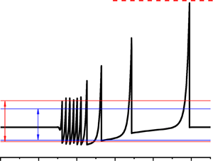
Figure 1. (a) The sharp increase in flow at Longmen Station on the Yellow River, China. (b) The shock waves on a uniform flow with  $\alpha = {\tau _o}/{(\rho g H \sin \theta )}= 0.3$ and
  $\beta = {\tan \theta UH}/{\nu } = 27$ obtained from a simulation by Liu & Mei (Reference Liu and Mei1994) for roll waves occurring at time
  $t (gH \sin \theta \tan \theta /\nu ) = 400$. Velocity and depth of the normal flow are
  $U$ and
  $H$; the yield stress and kinematic viscosity of the Bingham muddy fluid are
  $\tau _o$ and
  $\nu$, respectively. The slope angle of the channel is
  $\theta$. The data shown in (a) and (b) are reproduced from figures 9 and 10 of Liu & Mei (Reference Liu and Mei1994), respectively.
The spike of the flow in the Yellow River and the leading shock wave in the muddy fluid are striking. The present study, on the other hand, is derived from the clear-water model of Jeffreys (Reference Jeffreys1925), Dressler (Reference Dressler1949) and Brock (Reference Brock1967). However, the flow, the rheology, the theory, the stability condition of the uniform flow and the roll waves in the Yellow River studied by Liu & Mei (Reference Liu and Mei1994) are different. The clear-water model cannot explain the roll waves in the Yellow River with a mild slope but may be relevant to channel flow on a steep slope.
Most previous studies of roll waves in clear water have focused on the development of the waves over the full length of the channel (Zanuttigh & Lamberti Reference Zanuttigh and Lamberti2002; Balmforth & Mandre Reference Balmforth and Mandre2004; Que & Xu Reference Que and Xu2006; Richard & Gavrilyuk Reference Richard and Gavrilyuk2012; Ivanova et al. Reference Ivanova, Gavrilyuk, Nkonga and Richard2017). The present investigation examines a roll-wave group that occupies only part of the length of the channel. Such a roll-wave group of finite spatial extent was produced by a local disturbance. The flow upstream and downstream from the group was unperturbed, with a uniform depth  $H$ and uniform velocity
  $U$ as depicted in figure 2. The focus of our study was on the development of a front runner (FR) and the formation of a pack of trailing waves (TWs) in the wave group of finite spatial extent.

Figure 2. (a) A roll-wave group characterized by a FR and a pack of TWs. (b) The roll-wave group produced by a local disturbance in one simulation.
Roll waves are moving hydraulic jumps that advance with a speed greater than the velocity of the base flow. They are depth and velocity discontinuities in a shallow-water hydraulic model. Dressler (Reference Dressler1949) obtained a periodic solution of roll waves by matching the discontinuities with smooth profiles. Brock (Reference Brock1967) produced roll waves in the laboratory using two methods. The first method was to let the waves develop naturally from uniform flow. In the second method, the roll waves were produced by introducing finite-amplitude periodic disturbances at the inlet of an open channel. When roll waves were developed naturally from disturbances over the entire length of uniform flow, a process known as coarsening occurred – waves of greater amplitude tended to overtake others to produce waves of still greater amplitude. The physics behind the coarsening phenomenon is complicated and not well understood. On the other hand, when the disturbance was introduced locally at the inlet, the waves were thought to be periodic. But we found this to be true only after the FR exited the end of the channel. Brock (Reference Brock1967) measured the periodic part of the waves and found his measurements in agreement with the periodic solution of Dressler (Reference Dressler1949).
We conducted numerical simulations for the roll waves in clear water produced by inlet conditions similar to Brock's second method. Our simulations revealed the existence of a FR with an exceedingly large amplitude. We used a robust and accurate numerical scheme to capture the discontinuities in a shallow-water hydraulic model of the waves. We determined the advance of the FR towards its asymptotic limit and the formation of a periodic pack of TWs in the ever-expanding wave group of multiple fronts.
This paper has nine sections and two appendices, including an introduction and a formulation section. Section 3 presents the simulation profiles characterizing the roll waves with a FR and a pack of TWs. The relevant dimensionless parameters are introduced in this section. Section 4 correlates the simulation results using Dressler's periodic solution (DPS) as a guide. A comparison with the laboratory observations by Brock (Reference Brock1967) is given in § 5. Section 6 correlates the development of the FR in terms of a set of length scales. We show in § 7 that the rate of wave production was independent of the forms of the disturbances that produced the waves. Section 8 shows how celerity depends on wave amplitude. A summary and conclusions make up § 9. Finally, Appendix A provides a grid-refinement study. Appendix B presents the roll waves on a wavy channel bed in contrast to the roll waves produced by local disturbances.
2. Formulation
The governing equations that were solved for the depth  $h$ and the flow rate
  $q$ in a clear-water model of the roll waves were the shallow-water equations:
 \begin{gather} \frac{\partial h}{\partial t}+\frac{\partial q}{\partial x} = 0, \end{gather}
 \begin{gather} \frac{\partial q}{\partial t}+ \frac{\partial }{\partial x} \left[\frac{q^2}{h}+\frac{1}{2}g'h^2\right] = g' S_{o} h- \frac{c_f}{2} \frac{q {\left|q\right|}}{h^2}, \end{gather}
where  $S_o=$ channel slope =
  $\tan \theta$,
  $g'=g\cos \theta =$ gravity and
  $c_f=$ Chézy quadratic bed-friction coefficient. The spatial discretization of the equations for numerical simulation was the fifth-order weighted essentially non-oscillatory (WENO) scheme of Jiang & Shu (Reference Jiang and Shu1996). Numerical dissipation across the shock front was minimized by a nonlinear mapping procedure developed by Hendrick, Aslam & Powers (Reference Hendrick, Aslam and Powers2005). The third-order scheme of Pareschi & Russo (Reference Pareschi and Russo2005) was used for the time integration.
The simulation began with a base flow of depth  $H$ and velocity
  $U$ in a channel on a slope
  $S_o$. The base-flow Froude number was
  ${{Fr}} = U/\sqrt {g'H}$. The channel slope for the balance of gravity and friction in the base flow was
  $S_o = {c_f} {{Fr}}^2 / {2}$.
2.1. Three types of local disturbances with different durations
We produced shock waves by three local disturbances of amplitude  $\epsilon$ and period
  $T$, introduced at the inlet (where
  $x$ = 0), as follows:
 \begin{gather} \text{Type a}: \ h(0, t)=\left[1+\epsilon\sin \left(\frac{2 {\rm \pi}t}{T}\right)\right] H \quad \textrm{for} \ 0 < t < \infty. \end{gather}
 \begin{gather} \text{Type b}: \ h(0, t)=\left[1+\epsilon\sin \left(\frac{2 {\rm \pi}t}{T}\right)\right] H \quad \textrm{for} \ 0 < t \le T \ \textrm{and} \ h(0, t)={H} \quad \textrm{for} \ t > T. \end{gather}
 \begin{gather} \text{Type c}: \ h(0, t)=\left[1+\epsilon\sin \left(\frac{2 {\rm \pi}t}{T}\right)\right] H \quad \textrm{for} \ 0 < t \le \frac{1}{2} T \ \textrm{and} \ h(0, t)={H} \quad \textrm{for} \ t > \frac{1}{2} T. \end{gather}
The flow rate over the period of the disturbance was either
 \begin{equation} q(0,t)={{{Fr}}}\sqrt{g' h(0,t)^3} \end{equation}
by keeping the Froude number unchanged or
 \begin{equation} q(0,t)=UH \end{equation}
equal to the rate of the base flow. The disturbances that produced most simulations presented in this paper were subjected to the ‘constant- $Fr$’ constraint that specified the flow
  $q(0,t)$ by (2.6). The exceptions are in §§ 6, 7 and 8, where some disturbances were the result of the ‘constant-
 $q$’ constraint specified by (2.7).
The Type-a disturbance was continuous in time – introduced at the inlet in the same manner as in the laboratory experiments of Brock (Reference Brock1967). The Type-b and Type-c disturbances, in contrast, were of very short duration. The Type-b disturbance is one full sinusoid over the period from  $t=0$ to
  $t=T$. The Type-c disturbance is one half of a sinusoid from
  $t=0$ to
  $t=T/2$.
The Froude number  $Fr$ and the period of the disturbance
  $T$ selected for the simulations were identical to those in the laboratory experiments of Brock (Reference Brock1967).
3. Roll-wave profiles
The roll-wave profiles obtained from the simulation are shown in figures 3 and 4 for  $Fr = 3.71$ and 4.63, respectively. Each figure shows the waves produced by Type-a, Type-b and Type-c disturbances. The dimensionless parameters that define the nonlinear development of these waves are the base-flow Froude number
  $Fr = U/\sqrt {g'H}$ and the amplitude
  $\epsilon$ and the period
  $S_o TU/H$ of the inlet disturbance. The WENO scheme accurately captured the shock waves. We used 25 600 cells over the length of the channel to capture the peaks of the waves. The grid-refinement study in Appendix A shows that the fractional errors were about 1 % in capturing the peak amplitudes of the FR and 1 %–2 % in capturing other peaks.

Figure 3. The depth  $h/H$ profiles produced by (a) Type-a, (b) Type-b and (c) Type-c disturbances for
  $S_o T U/H=$ 6.08,
  $\epsilon =0.20$ and
  $Fr = 3.71$. The dashed lines represent the asymptotic limit of the FR. The thin red lines define DPS while the thin blue lines indicate those measured in the laboratory experiments of Brock (Reference Brock1967).

Figure 4. The flow-rate  $q/(UH)$ profiles produced by (a) Type-a, (b) Type-b and (c) Type-c disturbances for
  $S_o T U/H=$ 7.55,
  $\epsilon =0.20$ and
  $Fr = 4.63$. The dashed lines indicate the asymptotic limit of the FR. The thin red lines denote DPS.
Figure 3(a) shows the depth profiles  $h/H$ produced by the Type-a disturbance for the base flow with
  $Fr = 3.71$. Figure 4(a), on the other hand, shows the flow-rate profile
  $q/(UH)$, also produced by the Type-a disturbance, but for a higher Froude number of
  $Fr = 4.63$. The corresponding wave profiles produced by Type-b and Type-c inlet disturbances are shown in figures 3(b,c) and 4(b,c), for comparison with the profiles produced by the Type-a inlet disturbance. These profiles in figures 3 and 4 were obtained at the exactly the same times of
  $t/T=$ 23.6, 47.2, 70.8 and 94.4. The dimensionless periods of the disturbance were
  $S_oT U/H=$ 6.08 and 7.55 for the base flows with
  $Fr = 3.71$ and 4.63, respectively.
3.1. Front runner
The most striking shock wave produced by local disturbances was the FR. It was the leading shock wave with a much greater amplitude than the other shock waves in the ever-expanding group of shock waves developed from the instability.
For the base-flow Froude number  $Fr = 3.71$ as shown in figure 3, the shock-wave heights of the FR were
  $\hat {h}_{FR}/H=$ 2.79, 3.59, 3.94 and 4.07 at times
  $t/T =$ 23.6, 44.2, 70.8 and 94.4, respectively. The asymptotic limit was
  $\bar {h}/H=$ 4.20.
For the base flow with  $Fr = 4.63$ shown in figure 4, the peak flow rates of the FR were
  $\hat {q}_{FR}/(UH)=$ 5.97, 9.42, 11.12 and 11.86 at times
  $t/T =$ 23.6, 44.2, 70.8 and 94.4, respectively. The asymptotic limit for the flow rate was
  $\bar {q}/(UH)= 12.2$.
The dashed lines denote these asymptotic limits in the respective figures. We use the hat symbol  $\widehat {\ \ }$ to denote the peak amplitudes of the FR and the overline symbol
  $^{\overline {\ \ }}$ for their asymptotic limits.
Remarkably, the amplitudes of the FRs produced by the Type-a disturbance – shown in figures 3(a) and 4(a)– were the same as those shown in figures 3(b,c) and 4(b,c) produced by the Type-b and Type-c disturbances of much shorter duration. The slight discrepancies between the peak values produced by the three types of disturbances were less than 1 % – which is expected according to the grid-refinement study in Appendix A.
3.2. Jumps on arrival of the FR
The arrival of the FR produced not only a sudden jump in the depth  $h$ of the flow but at the same time a very significant increase in local velocity
  $u$. On arrival of the FR, the jump in flow rate,
  $q=uh$, above its normal rate,
  $UH$, was very large.
For  $Fr = 5.60$, the jumps were as high as
  $\bar {q}/UH=$ 20.2 times, in the asymptotic limit denoted by the dashed line in figure 5. At locations
  $S_o x /H=$ 400, 800, 1200 and 1600, the jumps in flow rates produced by the arrival of the FR were
  $\hat {q}/UH =$ 8.69, 13.7, 17.7 and 19.5, respectively. These many-fold increases above the normal are significant, and cannot be ignored in the study of related processes – such as river-bed erosion and wave-impact force on structures.

Figure 5. The sudden jump in the flow rate  $q$ over the normal
  $UH$ on arrival of the FR in a base flow with
  $Fr = 5.60$ and
  $\epsilon = 0.2$, for (a)
  $t_{FR}US_o/H= 271.36, x_{FR}S_o/H= 400$, (b)
  $t_{FR}US_o/H= 482.13, x_{FR}S_o/H= 800$, (c)
  $t_{FR}US_o/H= 672.73, x_{FR}S_o/H= 1200$ and (d)
  $t_{FR}US_o/H= 844.90, x_{FR}S_o/H= 1600$. (e) Arrival time.
3.3. Periodic TWs
The other development of significance was our observation of a periodic pack of TWs formed in the back of the roll-wave group. As shown in figures 3 and 4, the number of shock waves in the TW pack increased with time. The spatial extent of the pack also increased with time but the wavelength and amplitude stayed constant for all shock waves within the pack, whether the waves in the pack were produced by the Type-a, Type-b or Type-c inlet disturbances.
For  $Fr = 3.71$ as depicted by the thin red lines in figure 3, the crests and troughs of the TWs in the pack were
  $\hat {h}_{TW}/H \simeq$ 1.66 and
  $\check {h}_{TW}/H \simeq$ 0.65, respectively. These crests and troughs obtained from the simulations – denoted by the pair of thin red lines in the figure – were comparable to the wave-crest depth
  $\hat {h}_{exp} = 1.46$ and wave-trough depth
  $\check {h}_{exp}= 0.68$ measured by Brock (Reference Brock1967) in his laboratory experiments. The laboratory measurements are indicated by a pair of thin blue lines in the figures. The hat symbol ∧ denotes the wave-crest variables while the check symbol
  $\ \check{} $ denotes the wave-trough variables.
For  $Fr = 4.63$, the flow rates associated with the crests and troughs were
  $\hat {q}_{TW}/H \simeq$ 2.24 and
  $\check {q}_{TW}/H \simeq$ 0.45, respectively, as depicted by the thin red lines in figure 4.
4. Dressler's periodic solution
Dressler (Reference Dressler1949) constructed a periodic solution for roll waves by matching the smooth profiles between the depth and velocity jumps in a shallow-water hydraulic model. His analytical solution was exact, but he did not provide explicit equations for the wave parameters. We conducted calculations to find DPS based on his formulation. The lines in figure 6 are the results of the calculation results for the depths of the wave crest  $\hat {h}/H$ and wave trough
  $\check {h}/H$, the wave celerity
  ${c}/U$ and the wavelength
  $S_o \lambda /H$ as unique functions of the Froude number
  $Fr$ and the dimensionless wave period
  $T^*=S_o T U/H$.

Figure 6. The quasi-periodic TWs produced by Type-a disturbance compared with DPS for (a) the depths of the wave crest  $\hat {h}/H$ and wave trough
  $\check {h}/H$, (b) the wave celerity
  ${c}/U$ and (c) the wavelength
  $S_o \lambda /H$.
In the limit of infinitely long wavelength when  $T^*=S_o T U/H \rightarrow \infty$, the wave parameters
  $\bar {h}/H$,
  $\bar {u}/U$,
  $\bar {q}/(UH)$ and
  $\bar {c}/U$ are functions of the Froude number,
  $Fr$, as shown in figure 7. The overline symbol
  ${\overline {\ \ }}$ denotes the asymptotic limit of infinitely long wavelength.

Figure 7. Dressler's analytical solution for roll waves of infinitely long wavelength. The values of (a)  $\bar {h}/U$, (b)
  $\bar {u}/U$, (c)
  $\bar {q}/UH$ and (d)
  $\bar {c}/U$ for
  $Fr = 3.71$, 4.63 and 5.90 are highlighted using open circles.
4.1. Trailing waves and Dressler's periodic solution
The TWs obtained from our simulations were periodic because this matched well with DPS. Our simulations of the TW profiles shown in figures 2(b), 3 and 4 support this hypothesis of periodic TWs. The TW heights and the TW speed obtained for all simulations summarized in table 1 also support the hypothesis.
Table 1. Wave-crest heights, wave-trough depths and wave celerity obtained in our simulation for the TWs produced by Type-a disturbance ( $\hat {h}_{TW}$,
  $\check {h}_{TW}$,
  $c_{TW}$) compared with DPS (
 $\hat {h}_{PS}$,
  $\check {h}_{PS}$,
  $c_{PS}$).

The pairs of thin red lines in figures 2(b), 3 and 4 mark DPS. Table 1 shows the dimensionless wave-crest heights and wave-trough depths obtained for the TWs produced by the Type-a disturbance ( $\hat {h}_{TW}/H, \check {h}_{TW}/H$) compared with DPS (
 $\hat {h}_{PS}/H, \check {h}_{PS}/H$). The TW wave height
  ${(\hat {h}_{TW}-\check {h}_{TW})}$ and the wave height of DPS
  ${(\hat {h}_{PS}-\check {h}_{PS})}$ were essentially the same. The wave-height ratios,
  ${(\hat {h}_{TW}-\check {h}_{TW})}/{(\hat {h}_{PS}-\check {h}_{PS})}$, given in table 1 are almost equal to unity. The wave-speed ratios,
  $c_{TW}/c_{PS}$, in the bottom row of the table also are nearly equal to unity
The most comprehensive comparison – including wave speed  $c/U$ and wavelength
  $\lambda /H$ – between the TWs and DPS is shown figure 6. The filled and open symbols denote the TWs produced by the Type-a disturbance while the lines represent DPS. The simulation results for the TWs produced by the Type-b and Type-c disturbances – equally agreeing with DPS – are not shown in figure 6 because they overlapped with those symbols produced by the Type-a disturbance in the figure.
We conclude, therefore, that the amplitudes of all TWs produced by Type-a, Type-b and Type-c disturbances closely matched those of DPS. This conclusion was derived from simulations conducted for the same base-flow Froude number,  $Fr$, and disturbance period,
  $S_o T U/H$, as in Brock's laboratory experiments.
4.2. Front runner and long-wave limit of Dressler's solution
As the FR advances with increasing speed, it moves further and further away from the rest of the waves. The asymptotic state is a FR of infinitely long wavelength but finite amplitude. We assume the asymptotic limit of the FR to be the long-wave limit of Dressler's solution (LLDS). The dashed lines representing the LLDS in figures 2(b), 3, 4 and 5 support this hypothesis.
Figure 7 shows the LLDS for  $\bar {h}/H$,
  $\bar {u}/U$,
  $\bar {q}/(UH)$ and
  $\bar {c}/U$ as a function of the base-flow Froude number
  $Fr$. These values for
  $Fr = 3.71$, 4.63 and 5.60 are represented by the open circles on the curves shown in the figure, and are given also in table 2.
Table 2. The asymptotic values of the FR for  $\bar {h}/H$,
  $\bar {q}/(UH)$ and
  $\bar {c}/U$ assumed to be the LLDS.

5. Brock's laboratory experiments
Brock (Reference Brock1967) conducted two series of experiments in the laboratory. In the first series, the roll waves developed naturally from small disturbances distributed over the entire length of the channel. In the second series of experiments, the roll waves were produced by a periodic motion of a paddle at the inlet, like our Type-a disturbance. We do not know of what amplitude was the paddle motion in the experiment. But it was reported in Brock's thesis that the amplitude of the motion was adjusted so that the maximum and minimum depth did not change over a significant length of the laboratory channel.
Table 3 shows Brock's measurements of the wave-crest heights and wave-trough depths, ( $\hat {h}_{exp}$ and
  $\check {h}_{exp}$), and the TW wave-crest heights and wave-trough depths, (
 $\hat {h}_{TW}$ and
  $\check {h}_{TW}$), respectively. The Froude numbers in the laboratory experiments were
  $Fr = 3.71$, 4.63 and 5.60. The oscillation periods of the paddle motion were
  $S_o T U/H=$ 4.00, 6.08 and 7.94 in the experiments with
  $Fr = 3.71$,
  $S_o T U/H=$ 7.55, 13.4, 18.8 and 21.0 in the experiments with
  $Fr = 4.63$ and
  $S_o T U/H=$ 12.6, 19.9 and 29.0 in the experiments with
  $Fr = 5.60$.
Table 3. Brock's laboratory measurements ( $\hat {h}_{exp}$ and
  $\check {h}_{exp}$) compared with the TW wave-crest heights and wave-trough depths (
 $\hat {h}_{TW}$ and
  $\check {h}_{TW}$) obtained in our simulation.

The wave heights ( $\hat {h}_{exp}- \check {h}_{exp}$) obtained from the laboratory experiments were somewhat smaller than the heights of the TWs (
 $\hat {h}_{TW}- \check {h}_{TW}$). As shown in the last row of table 3, the ratios
  ${(\hat {h}_{exp}-\check {h}_{exp})}/{(\hat {h}_{TW}-\check {h}_{TW})}$, varying from 0.59 to 0.81, were smaller than unity. The laboratory wave heights were smaller than the TW heights produced by the Type-a disturbance.
In reality, the shock-wave front is not infinitely steep and is not perfectly reproduced by the shallow-water hydraulic model. The pressure variations were not hydrostatic, and velocity was not constant over the depth at the leading edge of the wavefronts. Brock (Reference Brock1967) and Richard & Gavrilyuk (Reference Richard and Gavrilyuk2012) modified the shallow-water model. Their models were different, but both modified models led to periodic solutions – with smaller amplitude than DPS – in better agreement with laboratory observation.
Brock measured the shock waves of uniform amplitude over the length of the channel. Thus, he could not have detected the existence of the FR as the leading shock waves were much greater in amplitude.
6. Growth of the FR towards its asymptotic limit
The FR advanced toward the asymptotic limit with increasing amplitude. We find that the rate of the increase diminished exponentially. The following relations – for the depth  $\hat {h}_{FR}$, the velocity
  $\hat {u}_{FR}$ and the celerity
  $\hat {c}_{FR}$ of the FR – fit well with the simulation profiles:
 $$\begin{gather} \hat{h}_{FR} = \bar{h} - \left[\bar{h} - \hat{h}_o\right] \exp \left[- \frac{x S_o}{\ell_h H}\right],\quad \hat{u}_{FR} = \bar{u} - \left[\bar{u} - \hat{u}_o\right] \exp \left[- \frac{x S_o}{\ell_u H}\right],\nonumber\\ \hat{c}_{FR} = \bar{c} - \left[\bar{c} - \hat{c}_o\right] \exp \left[- \frac{x S_o}{\ell_c H}\right]. \end{gather}$$
In these expressions,  $\ell _h$,
  $\ell _u$ and
  $\ell _c$ are the dimensionless longitudinal length scales that define the spatial growth of the FR towards its asymptotic values
  $\bar {h}$,
  $\bar {u}$ and
  $\bar {c}$, which were assumed to be the LLDS shown in figure 7.
Figure 8 shows how (6.1a–c) is a good fit of the simulation data obtained for  $Fr = 3.71$ and
  $\epsilon =$ 0.02 and 0.2. In this case for
  $Fr = 3.71$, the asymptotic values were
  $\bar {h}/H =$ 4.20,
  $\bar {u}/U =$ 1.67 and
  $\bar {c}/U =$ 1.89. The FR near the inlet was assumed to be equal to the amplitude of the inlet disturbance:
 \begin{equation} \hat{h}_o/H \simeq (1+\epsilon), \quad \hat{u}_o/U \simeq \sqrt{1+\epsilon} \quad \textrm{and} \quad \hat{c}_o/U \simeq {c}_{PS}/U. \end{equation}
The fit of the equation with the simulation data shown in the figure gives  $\ell _h= 377$,
  $\ell _u= 348$ and
  $\ell _c= 356$ for
  $\epsilon = 0.02$, and
  $\ell _h= 241$,
  $\ell _u=$ 248 and
  $\ell _c= 223$ for
  $\epsilon = 0.2$.

Figure 8. The approach of the FR towards its asymptotic state for  $Fr = 3.71$. The dotted line delineates the initial growth rate. The dashed line defines the asymptotic state. For
  $\epsilon = 0.02$, the best fit to the simulation data gives (a)
  $\ell _h=$ 377, (b)
  $\ell _u=$ 348 and (c)
  $\ell _c=$ 356. For
  $\epsilon = 0.2$, the best fit to the simulation data gives (d)
  $\ell _h=$ 241, (e)
  $\ell _u=$ 248 and (f)
  $\ell _c=$ 223.
It should be pointed out that the growth of the instability would be exponential if the disturbance were started from an infinitesimally small amplitude. On the other hand, in the nonlinear development of the instability, the growth rate was diminishing, and (6.1a–c) was for the nonlinear evolution. Therefore, the fits of the equation to data in figure 8(a–c) are good, but not perfect, because the amplitude  $\epsilon = 0.02$ is borderline, not large enough for the growth to be diminishing entirely. However, the fit to data in figure 8(d–f) is better because the disturbance amplitude
  $\epsilon = 0.2$ is sufficiently large to start the nonlinear development from the very beginning.
We have conducted a large number of simulations for the nonlinear development of the FR. Figure 9 summarizes the longitudinal length scales  $\ell _h$,
  $\ell _u$ and
  $\ell _c$ obtained from curve fitting of these simulation data for
  $Fr = 3.71$, 4.63 and 5.60 over a range of inlet-disturbance amplitudes varying from
  $\epsilon =$ 0.01 to 0.3. Two sets of simulation results are presented in the figure. The filled symbols represent those results obtained by specifying the flow of the disturbance
  $q(0,t)$ according to (2.6) for ‘constant
  $Fr$’. The open symbols, on the other hand, denote the results obtained by specifying
  $q(0,t)$ according to (2.7). In combinations of Type-a or Type-b or Type-c with constant
  $Fr$ or constant
  $q$, there were six different forms of disturbances. The nonlinear development of the FR was independent of the form of the disturbances. The length scales
  $\ell _h$,
  $\ell _u$ and
  $\ell _c$ – their dependence on
  $\epsilon$ – were the same for all FRs produced by the six different forms of disturbances.

Figure 9. The longitudinal length scales (a)  $\ell _h$, (b)
  $\ell _u$ and (c)
  $\ell _c$ and for three base-flow Froude numbers
  $Fr = 3.71$, 4.63 and 5.61, produced by Type-a, Type-b and Type-c disturbances over a range of inlet amplitudes varying from
  $\epsilon = 0.01$ to 0.3. The open symbols and the filled symbols denote the constant-
 $Fr$ and constant-
 $q$ disturbances, respectively.
7. Ever-expanding wave group produced by local disturbances
We emphasize that Type-b and Type-c disturbances were local instead of being distributed over the entire channel length. The wave groups produced by the local disturbances were ‘solitary’ because the base flow stayed undisturbed ahead and behind the groups. The instability continuously produced new waves adding to the wave group. Therefore, the number of waves in the group increased with time. The spatial extent of the group of roll waves also increased with time due to dispersion. The numbers of wave peaks shown in figure 3(b,c) for  $Fr = 3.71$ were 3, 5, 7 and 9 at time
  $t/T =$ 23.6, 47.2, 70.8 and 94.4, respectively. In figure 4(b,c) for
  $Fr = 4.63$, the numbers of peaks were 3, 6, 8 and 10 at time
  $t/T =$ 23.6, 47.2, 70.8 and 94.4, respectively.
Figure 10 shows the linear relation for the increase in the number of peaks,  $N_P$, with the dimensionless time,
  $S_o t U/H$. The increase rate depended on the Froude number but was unaffected by the shape of the local disturbances. The solid lines and dotted lines denote the results produced by the constant-
 $Fr$ and constant-
 $q$ disturbances, respectively. In combinations of Type-b and Type-c disturbances with constant
  $Fr$ and constant
  $q$, the four different shapes of the disturbances led to the same linear relation.

Figure 10. The number of peaks  $N_P$ in the wave group produced by (a) Type-b and (b) Type-c disturbances. The solid and dotted lines denote the results produced by the constant-
 $Fr$ and constant-
 $q$ disturbances, respectively.
By contrast, the roll waves on a wavy channel bed – produced by disturbances distributed over the entire length of the channel – are examined in Appendix B.
8. Celerity dependence on wave amplitude
Figure 11(a,b) shows the wave celerity of the FR and its dependence on the wave amplitude. The celerity increased with amplitude following an approximately linear relationship. The waves in the group dispersed because of the dependence of the celerity on wave amplitude. The celerity–amplitude relations were the same whether they were produced by Type-b or Type-c disturbances in combination with either the constant- $Fr$ or the constant-
 $q$ constraint.

Figure 11. The celerity–amplitude relation of the FR produced by (a) Type-b and (b) Type-c disturbances. The filled and open symbols denote the results produced by the constant- $Fr$ and constant-
 $q$ disturbances, respectively. The straight lines are the celerity–amplitude relations of the LLDS defined by the rates
  $\textrm {d}(c/U)/\textrm {d}(\hat {h}/H)=$ 0.0946, 0.0739 and 0.0638 for
  $Fr = 3.71$, 4.63 and 5.60, respectively. (c) The rate
  $\textrm {d}(c/U)/\textrm {d}(\hat {h}/H)$ as a function of
  $Fr$ of the LLDS.
We found almost the same celerity–amplitude relations in the solution of Dressler (Reference Dressler1949). The rate of increase in the celerity with the wave amplitude, in the LLDS, is a unique function of  $Fr$ as shown in figure 11(c). For
  $Fr = 3.71$, 4.63 and 5.60, the rates were
  $\textrm {d}(c/U)/\textrm {d}(\hat {h}/H)=$ 0.0946, 0.0739 and 0.0638, respectively. The straight lines in figure 11(a,b) – representing these rates of the LLDS – delineate well all results of our simulations produced by the four different disturbances.
A reviewer of this paper led us to a publication by Meza & Balakotaiah (Reference Meza and Balakotaiah2008), who studied the dynamics of nonlinear large-amplitude waves on vertically falling films for effects of viscosity and surface tension. The celerity–amplitude relationships of the vertical falling films also follow linear relationships independent of the forcing frequency and amplitude of the disturbance introduced at the inlet. Waves of exceedingly large amplitude also were produced in the vertical falling films and were characterized as ‘tsunami’ by Meza & Balakotaiah (Reference Meza and Balakotaiah2008). The similarity in the production of waves due to nonlinear instability between our clear-water roll waves and the vertical falling film is remarkable – despite the difference in gravity, viscosity and surface tension effects between the two problems.
Although the physics was different for the waves in Bingham muddy fluid, clear water and vertical falling films, the governing equations for these waves in various media are similar hyperbolic systems.
9. Summary and conclusion
We examined roll-wave groups of finite extent in clear water produced by local disturbances. The continuous production of waves leads to a linear increase in the number of waves within the group. Furthermore, the spatial extent of the group expands due to the dependence of celerity on the wave amplitude. The leading shock wave – the FR – is a wave of exceedingly large amplitude. Liu & Mei (Reference Liu and Mei1994) studied the roll wave as part of their instability theory of muddy fluid. The present investigation, on the other hand, is based on a clear-water model. We used a well-calibrated WENO scheme to study the ever-expanding number of shock waves produced by local disturbances. The FR advances with increasing speed and amplitude. But the amplitude has a limit which – in the clear-water model – is shown to be the LLDS. The nonlinear developments of the FR followed the same dependency on Froude number  $Fr$ and disturbance amplitude
  $\epsilon$ for all roll waves, irrespective of whether the waves were produced by a Type-a disturbance or by Type-b and Type-c disturbances of much shorter duration.
We note that there is currently no experimental evidence for this FR in clear water. The laboratory study of Brock (Reference Brock1967) did not detect the FR. Further investigation of the FR is needed. A laboratory search for the existence of the FR would be worthwhile since it appears to be universal, whether due to instability in clear water, muddy fluid or vertical falling films.
The focus of this paper was on the roll waves produced by local disturbances. The result of some simulations of the roll waves produced by the disturbance distributed over the length of the channel is nevertheless included in Appendix B.
Acknowledgement
We thank the reviewers for their insightful comments and suggestions that led to a significantly improved paper.
Declaration of interests
The authors report no conflict of interest.
Appendix A. Grid-refinement study
A grid-refinement study was conducted for the roll waves produced by the Type-b disturbance with  $S_oTU/H=6.08$ on a normal flow with a Froude number
  ${{Fr}}=3.71$. Figure 12(a) shows the simulation profiles comprised of nine peaks obtained at time
  $t/T=94.4$. The two profiles in the figure – obtained with
  $N$ = 25 600 cells and
  $N$ = 102 400 cells over the length of the channel – are virtually the same, visually indistinguishable.

Figure 12. (a) The roll-wave profiles obtained using cell numbers  $N=$ 25 600 and 102 400 for
  ${{Fr}}=3.71$ and
  $S_oTU/H=6.08$ at
  $t/T=94.4$. (b) The fractional error of the FR for
  $N=$ 12 800, 25 600, 51 200 and 102 400. The slope of the logarithmic plot is the order of convergence for the FR,
  $\hat {P}_{FR}=$ 1.139.
With three estimates  $(\hat {h}_{k-1}, \hat {h}_{k}, \hat {h}_{k+1})$ of a peak obtained from three sizes of the cell, the method of Stern et al. (Reference Stern, Wilson, Coleman and Paterson2001) is used to determine the true value by extrapolation to zero cell size using the formula
 \begin{equation} \hat{h}_{\Delta x \rightarrow 0}=\frac{r^{\hat{P}}\hat{h}_{k+1}-\hat{h}_{ k} }{r^{\hat{P}}-1}, \end{equation}
where  $r = {\Delta x_{k}}/{\Delta x_{k+1}}$ and
  $\hat {P}$ is the order of convergence determined by the formula
 \begin{equation} \hat{P}=\frac{1}{\ln r} \ln{\left[\frac{\hat{h}_{ \ k}-\hat{h}_{ k-1}}{\hat{h}_{ k+1}-\hat{h}_{ k}}\right]}. \end{equation}
 The numbers of computational cells over the length of the channel were  $N=$ 12 800, 25 600, 51 200 and 102 400 in the simulations conducted for the grid-refinement study in this appendix. Therefore,
  $r = {\Delta x_{k}}/{\Delta x_{k+1}} =$ 2. The peak amplitudes of the FR were
  $\hat {h}_{FR}/H=$ (4.025, 4.071, 4.095, 4.107) for
  $N=$ (12 800, 25 600, 51 200, 102 400). The true value of
  $\hat {h}_{\Delta x \rightarrow 0}$ was determined by extrapolation using (A1) and (A2) to zero grid size. Given three peak values
  $(\hat {h}_{k-1}, \hat {h}_{k}, \hat {h}_{k+1})$, the error relative to this true value was
  ${\left | \hat {h}_{k} - \hat {h}_{\Delta x \rightarrow 0} \right |}$. In percentage terms, the fractional error was
 \begin{equation} \widehat{FE} = \frac{{\left| \hat{h}_{k} - \hat{h}_{\Delta x \rightarrow 0} \right|} }{ \hat{h}_{\Delta x \rightarrow 0} } \times 100. \end{equation}
 Table 4 summarizes the results obtained from the grid-refinement simulations for the profiles produced by the Type-b disturbance with a period of  $S_oTU/H=6.08$ on a normal flow with a Froude number
  ${{Fr}}=3.71$. It gives the fractional error
  $\widehat {FE}_{FR}$ for the FR and
  $\widehat {FE}_i$ for the other peaks
  $i=2,3,\ldots, 9$ obtained by the method of Stern et al. (Reference Stern, Wilson, Coleman and Paterson2001). For cell number
  $N$ = 25 600, the fractional error in capturing the FR was
  $\widehat {FE}_{FR}=$ 0.9794 %. The order of convergence, evaluated using the three cell numbers
  $N=$ 25 600, 51 200 and 102 400, was
  $\hat {P}_{FR}=$ 1.139, which was consistent with the slope of the logarithmic plot shown in figure 12(b). For cell number
  $N$ = 25 600, table 4 shows that the fractional errors in capturing the other peaks,
  $\widehat {FE}_i$ for
  $i=2,3,\ldots, 9$, were in the range 1 %–2 %.
Table 4. The percentage fractional error  $\widehat {FE}_{FR}$ and
  $\widehat {FE}_i$ (
 $i=2,\,3,\ldots,9$), calculated using the extrapolation formulae of Stern et al. (Reference Stern, Wilson, Coleman and Paterson2001) for
  $N=$ 12 800, 25 600, 51 200 and 102 400;
  ${{Fr}}=3.71,\; S_oTU/H=6.08$ at time
  $t/T=94.4$.

We conducted a grid-refinement study also for the roll waves with Froude numbers  $Fr = 4.63$ (
 $S_oTU/H=7.55$,
  $t/T=94.4$) and 5.60 (
 $S_oTU/H=12.6$,
  $t/T=94.4$) produced by the Type-b disturbance. The fractional errors of these FRs with these Froude numbers – for cell number
  $N=$ 25 600 – were
  $\widehat {FE}_{FR}=$ 0.9087 % and 1.0724 %, respectively.
All simulations presented in this paper – other than the grid-refinement studies – were conducted using a cell number  $N$ = 25 600. We, therefore, concluded that the FR was captured with an accuracy of 99 %. The peaks of the TWs were captured with an accuracy of 98 %–99 %.
Appendix B. Roll waves on wavy channel bed
We examine in this appendix the development of the roll waves on a wavy channel bed where the channel slope  $S'_o$ is perturbed with a periodic disturbance of wavelength
  $\lambda _B$ and amplitude
  $\epsilon _B$ as follows:
 \begin{equation} S'_o=S_o(1+\epsilon_B \sin(2{\rm \pi} x/\lambda_B) ), \end{equation}
where  $S_o$ is the average of the channel slope.
The perturbation on the channel bed excited roll waves of wavelength  $\lambda _B$ and wave amplitude corresponding to DPS. The amplitude of DPS depends on wavelength. The thin red lines in figures 13 and 14 define the crest and trough of Dressler's periodic waves of wavelength
  $\lambda _B$.

Figure 13. Roll waves due to uniform flow at the inlet on a periodic channel bed. The channel slope is perturbed with an amplitude  $\epsilon _B=$ 0.10 and wavelength
  $S_o\lambda _B/H=$ (a) 1.57, (b) 6.28 and (c) 25.12. The normal-flow Froude number in this series of simulations was
  ${{Fr}}=$3.71.

Figure 14. Roll waves produced by Type-c inlet disturbance on the periodic channel bed. In this simulation, the amplitude and duration of the inlet disturbance were the same as those that led to the results in figure 3. The channel bed was exactly the same as the channel in figure 13. Wavelengths (a)  $S_o\lambda _B/H= 1.57$, (b)
  $S_o\lambda _B/H= 6.28$ and (c)
  $S_o\lambda _B/H=25.12$.
We compared the roll waves on the same channel bed for different flows of the same normal-flow Froude number. Figure 13 shows the wave produced by the wavy channel bed without inlet disturbance. Figure 14, on the other hand, shows the roll waves on the same wavy bed with a Type-c inlet disturbance. The profiles in figures 13 and 14 are comparable with figure 3(c) as the waves shown in these three figures had the same Froude number of  $Fr = 3.71$.
The interaction between the waves produced by the inlet disturbance and the wavy channel bed led to a complex system of waves. We nevertheless can identify a maximum wave-crest height  $\hat {h}_{max}$ for each relatively complex wave profile shown in figure 14. Figure 15 shows the development of the maximum crest height
  $\hat {h}_{max}/H$ with distance
  $S_o x/H$. The interaction with the Type-c inlet disturbance with the wavy bed led to the maximum height
  $\hat {h}_{max}$ comparable with the FR amplitude
  $\hat {h}_{FR}$ of the waves on the smooth bed. A more noticeable interaction, however, is shown in figures 14(c) and 15(c) for the wavy bed with the large wavelength
  $S_o\lambda _B/H=$ 25.12.

Figure 15. The maximum height,  $\hat {h}_{max}$, of the wave crests shown in figure 14. The dashed red line delineates the FR amplitude
  $h_{FR}$ for the wave profiles shown in figure 3(c) for the same Froude number
  $Fr = 3.71$. The dotted line is the asymptotic LLDS. Wavelengths (a)
  $S_o\lambda _B/H= 1.57$, (b)
  $S_o\lambda _B/H= 6.28$ and (c)
  $S_o\lambda _B/H=25.12$.


