


1. Introduction
Laminar-to-turbulent transition may occur in boundary-layer flow after instability modes in the laminar region interact each other. Challenges in assessing the transition mechanism arise owing to the nonlinear (or energetic) interaction. Various transition routes were suggested for wall-bounded flow by Morkovin (Reference Morkovin1969) about five decades ago. Disturbances outside the boundary layer are converted to a primary instability inside the boundary layer through the receptivity process, secondary instability normally occurs as the primary instability grows to sufficiently large amplitude and promotes modal interactions. The secondary instability (here, subharmonic resonance) occurs following the amplification of a three-dimensional (3-D) wave initiated by a two-dimensional (2-D) Tollmien–Schlichting (TS) wave, i.e. the primary instability mode of the Orr–Sommerfeld flow field. The 3-D wave has one-half the frequency of the fundamental TS wave.
Significant progress has been made in the understanding of secondary instabilities, which have been well reviewed in Herbert (Reference Herbert1988), Kachanov (Reference Kachanov1994), Saric, Reed & White (Reference Saric, Reed and White2003) and Schmid (Reference Schmid2007). Subharmonic secondary instability has been investigated extensively, using theoretical approaches (Craik Reference Craik1971; Herbert Reference Herbert1984, Reference Herbert1988; Wu Reference Wu2019), experimental studies (Kachanov & Levchenko Reference Kachanov and Levchenko1984; Corke & Mangano Reference Corke and Mangano1989; Borodulin, Kachanov & Koptsev Reference Borodulin, Kachanov and Koptsev2002; Würz et al. Reference Würz, Sartorius, Kloker, Borodulin, Kachanov and Smorodsky2012a) and numerical investigation (El-Hady Reference El-Hady1988; Nayfeh & Masad Reference Nayfeh and Masad1990; Bertolotti, Herbert & Spalart Reference Bertolotti, Herbert and Spalart1992; Joslin, Streett & Chang Reference Joslin, Streett and Chang1993; Xu, Lombard & Sherwin Reference Xu, Lombard and Sherwin2017; Jee, Joo & Lin Reference Jee, Joo and Lin2018; Kim et al. Reference Kim, Lim, Kim, Jee, Park and Park2019, Reference Kim, Lim, Kim, Jee and Park2020). The current study focuses on the subharmonic resonance in the natural transition path for incompressible flow. Other transition routes including a non-modal interaction leading to transient growth and bypass transition are well reviewed by Schmid (Reference Schmid2007) and Durbin & Wu (Reference Durbin and Wu2007), respectively.
It is well recognised that the early stage of secondary instability involves the parametric resonance of the subharmonic mode with respect to the basic flow composed of steady slow-varying laminar flow and the 2-D fundamental mode (Herbert Reference Herbert1984, Reference Herbert1988; El-Hady Reference El-Hady1988; Nayfeh & Masad Reference Nayfeh and Masad1990). The parametric resonance of the subharmonic mode can be analysed with Floquet theory applied to the basic flow. Among several parameters of the instability modes affecting the growth of the subharmonic mode, key parameters have been identified as the local Reynolds number of the basic flow, the amplitude of the fundamental mode and the spanwise wavenumber of the subharmonic mode (Herbert Reference Herbert1988). Floquet analysis for subharmonic resonance (Herbert Reference Herbert1984; Herbert, Bertolotti & Santos Reference Herbert, Bertolotti and Santos1987; Nayfeh & Masad Reference Nayfeh and Masad1990) has been validated for the well-controlled experiments of Klebanoff, Tidstrom & Sargent (Reference Klebanoff, Tidstrom and Sargent1962) and Kachanov & Levchenko (Reference Kachanov and Levchenko1984).
Despite a vast amount of literature on subharmonic resonance, a complete understanding of the nonlinear interaction between the fundamental and the subharmonic modes has not been achieved. In particularly, the nonlinear interaction influenced by the phase difference between the two waves has not gained enough attention in the research community. Recently, Park et al. (Reference Park, Park, Kim, Lim, Kim and Jee2021) reproduced the phase-dependent subharmonic resonance observed in the experiment of Borodulin et al. (Reference Borodulin, Kachanov and Koptsev2002) using nonlinear parabolised stability equation analysis (PSE). Yet, the effect of the phase difference on the subharmonic resonance has not been fully identified. Note that previous studies (Borodulin et al. Reference Borodulin, Kachanov and Koptsev2002; Würz et al. Reference Würz, Sartorius, Kloker, Borodulin, Kachanov and Smorodsky2012a; Park et al. Reference Park, Park, Kim, Lim, Kim and Jee2021) were still confined to the pre-turbulence region due to experimental (Borodulin et al. Reference Borodulin, Kachanov and Koptsev2002; Würz et al. Reference Würz, Sartorius, Kloker, Borodulin, Kachanov and Smorodsky2012a) and numerical (Park et al. Reference Park, Park, Kim, Lim, Kim and Jee2021) constraints.
The goal of the current study is to improve the understanding of the phase effect on boundary-layer transition, covering a wide transition range from the early stage of primary and secondary instabilities to turbulent flow. To achieve such a comprehensive investigation, three numerical methods are judiciously incorporated: Floquet analysis, PSE and large-eddy simulation (LES). Floquet analysis provides a resonating subharmonic mode (secondary instability) with respect to the fundamental mode (primary instability). An in-house code has been developed for the current Floquet analysis based on previous studies (El-Hady Reference El-Hady1988; Nayfeh & Masad Reference Nayfeh and Masad1990). Because Floquet analysis is limited to the resonant subharmonic mode (resonant phase difference), PSE is chosen as a higher-fidelity stability analysis for non-resonant phase differences. Because PSE can handle the nonlinearity and non-parallelism of the disturbance equations, the instability evolution affected by the phase can be investigated in the nonlinear transition region. A well-validated nonlinear PSE code by Park & Park (Reference Park and Park2013, Reference Park and Park2016); Park et al. (Reference Park, Park, Kim, Lim, Kim and Jee2021) is used in the current study. Although PSE is an effective method for stability analysis in a pre-turbulence region, it is computationally prohibitive in turbulent flow. The authors have developed an LES method coupled with stability analysis (Kim et al. Reference Kim, Lim, Kim, Jee, Park and Park2019, Reference Kim, Lim, Kim, Jee and Park2020; Lim et al. Reference Lim, Kim, Kim, Jee and Park2021) for a cost-effective and high-fidelity simulation of a transitional boundary layer. This LES method is used for a complete turbulent transition here, and the transition location controlled by the initial phase difference is quantified. It should be noted that the current LES approach (Kim et al. Reference Kim, Lim, Kim, Jee, Park and Park2019, Reference Kim, Lim, Kim, Jee and Park2020) provides direct numerical simulation (DNS) fidelity in the laminar region where disturbances are deterministic.
In § 2, three methods, Floquet analysis, PSE and LES are described. The validation of the current Floquet analysis is discussed in § 3.1. The effect of the phase difference on the subharmonic resonance is thoroughly investigated using PSE and LES in § 3.2 and 3.3, respectively. The mechanism of the phase synchronisation from anti-resonant conditions is discussed in § 3.4. Because the amplitude of the fundamental mode (not the subharmonic mode) is a major parameter to affect the subharmonic resonance, amplitude effects on anti-resonance and phase synchronisation are further studied in § 3.5. A summary and conclusions are given in § 4.
2. Methods
Three numerical methods are used in this study. Parametric resonance of the subharmonic oblique wave is investigated using Floquet analysis. The PSE is conducted to study the effect of the phase difference on the parametric resonance. The LES is carried out to simulate complete transition to turbulent boundary layer. Floquet analysis, PSE and LES are briefly discussed in §§ 2.1, 2.2 and 2.3, respectively.
In this study, a total variable  $\check {\psi }$ is decomposed to the undisturbed part
  $\varPsi$ and the disturbance
  $\psi$.
 \begin{equation} \check{\psi} = \varPsi + \psi. \end{equation}
The Cartesian coordinate system is used with the streamwise  $x$, wall-normal
  $y$ and spanwise
  $z$ direction, along with the corresponding velocity components
  $u$,
$u$,  $v$ and
  $w$. Dimensionless variables are obtained with the length scale
  $\tilde {\delta }_r(R=R_o)$, the free-stream velocity
  $\tilde {U}_\infty$ and the dynamic pressure
  $\tilde {\rho }\tilde {U}^2_\infty$, where the local length variable is
  $\tilde {\delta }_r=\sqrt {\tilde {x}_r \tilde {\nu } / \tilde {U}_\infty }$,
  $\tilde {x}_r$ is the distance from the leading edge of a flat plate,
  $\tilde {\nu }$ is kinematic viscosity, the local Reynolds number is
  $R=\tilde {U}_\infty \tilde {\delta }_r/\tilde {\nu }=\sqrt {\tilde {U}_\infty \tilde {x}_r/\tilde {\nu }}=\sqrt {Re_x}$, the reference
  $R$ is
  $R_o = 400$ and
  $\tilde {\rho }$ is the fluid density. The tilde denotes a dimensional variable.
2.1. Floquent analysis
Floquet analysis is based on a parametric formulation which describes a secondary instability for a given primary instability (Herbert Reference Herbert1984; Herbert et al. Reference Herbert, Bertolotti and Santos1987; El-Hady Reference El-Hady1988; Nayfeh & Masad Reference Nayfeh and Masad1990). The current Floquet analysis, briefly described here, adopts the approach of Nayfeh & Masad (Reference Nayfeh and Masad1990) and El-Hady (Reference El-Hady1988) instead of the stream-function approach of Herbert (Reference Herbert1984) and Herbert et al. (Reference Herbert, Bertolotti and Santos1987).
The governing equations of a disturbance ( $u, v, w, p$) for an undisturbed basic flow (
 $U, V$) are written as
 $$\begin{gather} \frac{\partial u}{\partial x} + \frac{\partial v}{\partial y} + \frac{\partial w}{\partial z} =0, \end{gather}$$
 $$\begin{gather}\frac{\partial u}{\partial t} + U\frac{\partial u}{\partial x} + v\frac{\partial U}{\partial y} + \frac{\partial p}{\partial x} - \frac{1}{R_o}\nabla^2 u + \left[u\frac{\partial U}{\partial x} + V\frac{\partial u}{\partial y} \right] + \mathbb{N}_u =0, \end{gather}$$
 $$\begin{gather}\frac{\partial v}{\partial t}+U\frac{\partial v}{\partial x}+\frac{\partial p}{\partial y} - \frac{1}{R_o}\nabla^2 v + \left[ u\frac{\partial V}{\partial x} + V\frac{\partial v}{\partial y} + v\frac{\partial V}{\partial y} \right] + \mathbb{N}_v = 0, \end{gather}$$
 $$\begin{gather}\frac{\partial w}{\partial t} + U\frac{\partial w}{\partial x} + \frac{\partial p}{\partial z} - \frac{1}{R_o}\nabla^2 w + \left[ V\frac{\partial w}{\partial y} \right] + \mathbb{N}_w =0, \end{gather}$$
where the square-bracket terms represent the non-parallel nature of the basic flow. The nonlinear terms of the disturbance  $\mathbb {N}$ are negligible here.
The instability analysis involves two steps: primary and secondary instability. The primary instability analysis provides a 2-D fundamental TS wave for a given basic laminar flow, whereas the secondary instability analysis (Floquet) yields a 3-D subharmonic wave for a given basic flow in which the 2-D wave is additionally included. The current analysis is summarised in table 1 with a brief description below.
Table 1. Basic flow and disturbance for each analysis of primary and secondary instability.

For the primary instability of a boundary layer, we consider the basic flow
 \begin{equation} \left\{ U, V \right\} = \left\{ U_L(y), 0 \right\}, \end{equation}
where  $U_L$ is the laminar solution without any disturbance (here the Blasius solution). Then, a fundamental planar TS wave can be written as
 \begin{equation} \left\{ u,v,p \right\} = \left\{ \zeta_1(y), \zeta_3(y), \zeta_4(y) \right\} \exp \left[ \textrm{i} \left( \alpha x -\omega t \right) \right] + \text{c.c.}, \end{equation}
where the notation c.c. indicates the complex conjugate. The functions  $\zeta _1(y)$,
  $\zeta _3(y)$ and
  $\zeta _4(y)$ are the mode shape of the fundamental TS components
  $u$,
$u$,  $v$ and
  $p$, respectively. For a spatially evolving disturbance, the complex wavenumber
  $\alpha$ and the real angular frequency
  $\omega$ are used.
To obtain the subharmonic oblique wave in the Floquet analysis, the basic flow (2.5) includes both the laminar flow and the fundamental 2-D TS wave.
 $$\begin{gather} U = U_L(y) + A \left[ \zeta_1 (y) \exp(\textrm{i}\theta) + \zeta^*_1 (y) \exp(-\textrm{i}\theta) \right], \end{gather}$$
 $$\begin{gather}V = A \left[ \zeta_3 (y) \exp(\textrm{i}\theta) + \zeta^*_3 (y) \exp(-\textrm{i}\theta) \right], \end{gather}$$
where  $A$ is the r.m.s. amplitude of the fundamental TS wave,
  $\zeta ^*$ is the complex conjugate of the function
  $\zeta$ and
  $\theta (x,t)=\mathrm {Re}(\alpha )x-\omega t$. The notations
  $\mathrm {Re}$ and
  $\mathrm {Im}$ indicate the real and the imaginary part of a complex variable, respectively. Floquet theory suggests that the approximate solution of (2.2) for the given basic flow of (2.5) can be written as
 $$\begin{gather} \left\{
\begin{array}{@{}c@{}} u_{1/2} \\ v_{1/2} \\ p_{1/2}
\end{array} \right\} = \left[ \left\{
\begin{array}{@{}c@{}} \eta_1(y) \\ \eta_3(y) \\ \eta_4(y)
\end{array} \right\} \exp(\textrm{i}\theta/2) + \left\{
\begin{array}{@{}c@{}} \eta_7(y) \\ \eta_9(y) \\ \eta_{10}(y)
\end{array} \right\} \exp(-\textrm{i}\theta/2) \right]
\cos(\beta z) \exp(\gamma x),
\end{gather}$$
$$\begin{gather} \left\{
\begin{array}{@{}c@{}} u_{1/2} \\ v_{1/2} \\ p_{1/2}
\end{array} \right\} = \left[ \left\{
\begin{array}{@{}c@{}} \eta_1(y) \\ \eta_3(y) \\ \eta_4(y)
\end{array} \right\} \exp(\textrm{i}\theta/2) + \left\{
\begin{array}{@{}c@{}} \eta_7(y) \\ \eta_9(y) \\ \eta_{10}(y)
\end{array} \right\} \exp(-\textrm{i}\theta/2) \right]
\cos(\beta z) \exp(\gamma x),
\end{gather}$$
 $$\begin{gather}w_{1/2} = \left[ \eta_5(y) \exp(\textrm{i}\theta/2) + \eta_{11}(y) \exp(-\textrm{i}\theta/2) \right] \sin(\beta z) \exp(\gamma x), \end{gather}$$
where the subharmonic wavenumber in the streamwise direction is  $\alpha _{1/2}=\mathrm {Re}(\alpha )/2$, the subharmonic frequency is
  $\omega _{1/2}=\omega /2$ (so,
  $\theta /2=\alpha _{1/2}x-\omega _{1/2}t$), the spanwise wavenumber of the subharmonic mode is
  $\beta$ and the eigenvalue
  $\gamma$ is real here. Further details are documented in Appendix A, including the exact equation for each analysis, boundary conditions and the computational method for the eigenvalue problems.
2.2. PSE
The method of PSE is an efficient way to treat weakly nonlinear regions where parametric resonance occurs. The amplitude of the subharmonic mode remains small so that the back influence of the subharmonic mode on the fundamental mode is negligible. A formal approach of PSE is to decompose the disturbance  $\psi$ into a fast-varying oscillatory-wave part and a slow-varying shape function, using Fourier expansion, as written in (2.7).
 \begin{equation} \psi(x,y,z,t) = \sum_{m={-}N_m}^{N_m} \sum_{n={-}N_n}^{N_n} \hat\psi_{(m,n)} (x, y) \exp \left[\textrm{i} \left\{ \int_{x_{0}}^{x} \alpha_{(m,n)}(s)\,\textrm{d} s + n \beta z - \tfrac{1}{2} m \omega t \right\} \right], \end{equation}
where the shape function  $\hat \psi _{(m,n)}$ is a complex function, the streamwise wavenumber
  $\alpha _{(m,n)}$ is a complex number the spanwise wavenumber
  $\beta$ is a real number. The subscript
  $m$ and
  $n$ indicates the temporal and spanwise modes, respectively. The wavenumber
  $\alpha _{(2,0)}$ of the fundamental TS wave corresponds to the wavenumber
  $\alpha$ in (2.4). The subharmonic wavenumber
  $\alpha _{(1,1)}$ is associated with the notations
  $\alpha _{1/2}$ and
  $\gamma$ in (2.6), i.e.
  $\alpha _{(1,1)}=\alpha _{1/2} - \textrm {i} \gamma$. The spatial growth rate of the subharmonic mode is
  $\mathrm {Im}(\alpha _{(1,1)})=-\mathrm {Re}(\gamma )$.
A set of partial differential equations for the shape functions with the unknown variable  $\alpha _{(m,n)}$ is obtained for a given frequency (here the fundamental frequency
  $\omega$) and the spanwise wavenumber
  $\beta$. These equations are parabolised and numerically solved in the PSE code developed in Park & Park (Reference Park and Park2013, Reference Park and Park2016). Nonlinear PSE is conducted with
  $N_m=6$ and
  $N_n=3$, keeping a total of 28 modes including the mean distortion
  $(0,0)$ mode, in the domain of
  $400 \leq R \leq 700$. A fourth-order central scheme and a second-order backward scheme are used for the wall-normal and the streamwise direction, respectively. Uniform grids with 107 points are used in the streamwise direction. At least 80 points are placed in the boundary layer with a total 220 points in the wall-normal domain, extending to
  $200 \tilde {\delta }_r$. Further details of the PSE code and numerical approaches are documented in Park & Park (Reference Park and Park2013, Reference Park and Park2016), Kim et al. (Reference Kim, Lim, Kim, Jee, Park and Park2019) and Park et al. (Reference Park, Park, Kim, Lim, Kim and Jee2021).
It should be noted that the PSE code is based on the compressible form of the disturbance equation. To approximate the incompressible boundary layer, the mean flow of very low free-stream speed whose Mach number is 0.0269 is chosen (i.e.  $9.16\ \textrm {m}\,\textrm {s}^{-1}$ with the standard atmospheric condition at sea level). At this Mach number condition and at the corresponding mean flow conditions, the density and temperature fluctuations behave as redundant variables in the PSE analysis. Although the compressible formulation is used and all terms are kept, the results can be regarded as nearly identical to those obtained from the incompressible formulation as they have been validated through many cases (Bertolotti et al. Reference Bertolotti, Herbert and Spalart1992; Chang et al. Reference Chang, Malik, Erlebacher and Hussaini1993; Gao, Park & Park Reference Gao, Park and Park2011; Park & Park Reference Park and Park2013). In addition, the results from the Floquet theory are used as the inlet boundary conditions for the PSE as well as LES. For the initial condition of PSE, the pressure and velocity disturbances are set as the Floquet theory results, while the density and temperature disturbances are set as zero. As a consequence, there might be a small difference in comparison with the solution with the compressible formulation. However, this discrepancy is also almost negligible owing to the very low Mach number considered.
2.3. LES
Because neither Floquet analysis nor PSE are efficient for incorporating higher instability in the late stage of transition, LES is conducted to model the boundary-layer flow well into a fully turbulent state. The total variable  $\check {\psi }$ is decomposed to the spatially filtered
  $\bar \psi$ and the filtered residual part
  $\psi '$ for LES.
 \begin{equation} \check{\psi} = \bar{\psi} + \psi'. \end{equation}
Note that there is no distinction between  $\check {\psi }$ and
  $\bar \psi$ in the computation of laminar flow because LES is essentially DNS in this case (Kim et al. Reference Kim, Lim, Kim, Jee, Park and Park2019, Reference Kim, Lim, Kim, Jee and Park2020). The residual part
  $\psi '$ is a turbulence fluctuation, so
  $\psi '=0$ in the pre-transition region where the deterministic disturbance
  $\psi$ (see (2.1)) is well resolved with the current fine grid.
The filtered incompressible dimensionless Navier–Stokes equations are written as (2.9).
 $$\begin{gather} \frac{\partial \bar{u}_i}{\partial x_i} = 0, \end{gather}$$
 $$\begin{gather}\frac{\partial \bar{u}_j}{\partial t} + \frac{\partial}{\partial x_i} \left( \bar{u}_i \bar{u}_j \right) = \frac{1}{R} \frac{\partial ^2 \bar{u}_j}{\partial x_i \partial x_i} - \frac{\partial \tau^{r}_{ij}}{\partial x_i} - \frac{\partial \bar{p}}{\partial x_j}, \end{gather}$$
 $$\begin{gather}\tau^r _{ij} ={-}2\nu _t \bar{S}_{ij}, \end{gather}$$
 $$\begin{gather}\bar{S}_{ij} = \frac{1}{2} \left( \frac{\partial \bar{u}_i}{\partial x_j} + \frac{\partial \bar{u}_j}{\partial x_i} \right), \end{gather}$$
where the residual stress tensor  $\tau ^r _{ij}$ is modelled to be linearly proportional to the resolved strain rate
  $\bar {S}_{ij}$. The turbulence viscosity
  $\nu _t$ is obtained with the wall-adapting local eddy-viscosity model (see Nicoud & Ducros Reference Nicoud and Ducros1999). The model coefficient is
  $C_w=0.5$ as suggested in Nicoud & Ducros (Reference Nicoud and Ducros1999) and tested in the transitional boundary layer in Kim et al. (Reference Kim, Lim, Kim, Jee, Park and Park2019, Reference Kim, Lim, Kim, Jee and Park2020). The sub-grid-scale turbulence model is judiciously chosen for wall-resolved LES in the transitional boundary layer (Kim et al. Reference Kim, Lim, Kim, Jee and Park2020), the model is properly activated only in the very late transition stage and the subsequent turbulent region in the current simulation.
The computational domain is depicted in figure 1. At the LES inlet, the fundamental and subharmonic modes are assigned to the laminar solution. The convective outlet is applied at the exit boundary, and no-slip condition at the wall. The fine grid of Kim et al. (Reference Kim, Lim, Kim, Jee, Park and Park2019) is used here with a small enough time step  $\Delta _t=({1}/{256})({2{\rm \pi} }/{\omega })$ where
  $\omega$ is the angular frequency of the fundamental mode. Further details on the LES approach can be found in Kim et al. (Reference Kim, Lim, Kim, Jee, Park and Park2019, Reference Kim, Lim, Kim, Jee and Park2020).

Figure 1. Schematic diagram of the LES computational domain.
2.4. Inlet conditions for PSE and LES
Both PSE and LES computations require a disturbance at the inlet boundary, which is located at  $R=400$. The 2-D TS wave and the pair of the 3-D oblique waves are obtained from the current Floquet analysis. Following the Floquet analysis of Herbert et al. (Reference Herbert, Bertolotti and Santos1987), which has been validated for the experiment of Kachanov & Levchenko (Reference Kachanov and Levchenko1984), the angular frequency of the 2-D wave is
  $\omega =0.0496$ and the spanwise wavenumber of the 3-D wave is
  $\beta =0.132$ based on the current non-dimensionalisation. These two parameters can be rewritten as
  $F=\omega / R \times 10^6=124$ and
  $b=\beta / R \times 10^3=0.33$, respectively, which are also commonly used in the literature. The r.m.s. amplitudes of the 2-D wave and the 3-D wave are
  $A_{(2,0)}=4.0\times 10^{-3}$ and
  $A_{(1,1)}=1.64\times 10^{-5}$, respectively, at the inlet, where the free-stream velocity is used for the scaling. At the LES and PSE inlet boundary, 2-D fundamental and 3-D subharmonic modes are added to the laminar solution; namely a zero-pressure-gradient flat-plate flow at
  $R=400$.
The current Floquet analysis provides the mode shape of the fundamental (2-D TS wave)  $\zeta$ and the subharmonic (3-D oblique wave)
  $\eta$ modes, as shown in figure 2. The amplitude of each mode is scaled with the maximum value of each mode. The
  $u$ component dominates both the fundamental and subharmonic modes. The amplitude peak of the fundamental and subharmonic modes is located at approximately one quarter of the boundary-layer thickness. The phase profile of the fundamental mode
  $\zeta _1$ is relatively constant near the amplitude peak, whereas the phase of
  $\eta _1$ changes continuously.

Figure 2. The fundamental and the subharmonic modes obtained from the current Floquet analysis at  $R=400$. (a) Amplitude
  $|\zeta |/\max (|\zeta |)$. (b) Phase
  $\phi _{(2,0)}=\arg (\zeta )$. (c) Amplitude
  $|\eta |/\max (|\eta |)$. (d) Phase
  $\phi _{(1,1)}=\arg (\eta )$.
The phase difference  $\Delta \phi$ between the fundamental and the subharmonic modes is defined as (2.10), following experimental studies of Borodulin et al. (Reference Borodulin, Kachanov and Koptsev2002); Würz et al. (Reference Würz, Sartorius, Kloker, Borodulin, Kachanov and Smorodsky2012a).
 \begin{equation} \Delta \phi = \tfrac{1}{2} \phi_{(2,0)} - \phi _{(1,1)} \quad \text{at} \ y_{(1,1),max}, \end{equation}
where  $y_{(1,1), max}$ is the location for the amplitude peak of the subharmonic mode which is
  $y_{(1,1), max}=1.43$ at the inlet. The initial phase difference between the fundamental and subharmonic modes is
  $\Delta \phi _{in}=130 ^{\circ }$ from the Floquet analysis. In the current PSE and LES computations,
  $\Delta \phi _{in}$ varies in the periodic range of
  $180^{\circ }$ to allow investigation of the effect of the phase difference on the secondary instability and eventually on turbulent transition. The subharmonic phase is shifted with respect to the given fundamental mode. There is no distinction between the phase lead and lag results in the periodicity of
  $180^{\circ }$ for the phase difference.
3. Results
The effect of the modal phase on the growth of the secondary instability (here, the subharmonic mode) is investigated using three approaches, i.e. Floquet analysis, PSE and LES. The baseline case is the subharmonic resonance in the zero-pressure-gradient boundary layer on a flat plate, which was experimentally studied by Kachanov & Levchenko (Reference Kachanov and Levchenko1984). The current Floquet analysis, validated against the experimental (Kachanov & Levchenko Reference Kachanov and Levchenko1984) and the numerical data (Herbert et al. Reference Herbert, Bertolotti and Santos1987) in § 3.1, provides a resonating subharmonic mode for the given basic flow which consists of laminar flow and the fundamental mode (2-D TS wave). Because of the nature of the eigenvalue problem explored in the Floquet analysis, other methods are required for less resonating conditions affected by the modal phase. Here, PSE and LES are used. The phase effect is first discussed with PSE in § 3.2 and then with LES in § 3.3. A further investigation on the transition location delay affected by the phase and the resonance mechanism from an anti-resonant initial condition is included in § 3.4. Because the fundamental amplitude is one of major parameters affecting the subharmonic resonance, it is speculated that the evolution of the subharmonic mode from the anti-resonant initial condition is also affected by the fundamental amplitude, not the subharmonic amplitude. Such amplitude effects are assessed in § 3.5.
3.1. Validation of instability analysis
The current instability analysis consists of two parts, one for the primary instability (2-D fundamental TS wave) and the other for the secondary instability (3-D subharmonic oblique wave). The eigenvalue problem of each analysis is summarised in table 1 along with the given basic flow. Floquet analysis provides the most unstable mode for the subharmonic oblique wave, yielding the mode shape  $\eta$ and the exponent
  $\gamma$ whose positive real value is the spatial growth rate of the subharmonic wave.
The mode shape and the amplitude growth of the subharmonic mode are compared with the experimental data of Kachanov & Levchenko (Reference Kachanov and Levchenko1984) and the Floquet analysis of Herbert et al. (Reference Herbert, Bertolotti and Santos1987), as shown in figure 3. The amplitude growth is obtained, using the integration
 $$\begin{gather} \frac{A_{(2,0)}(x)}{A_{(2,0)}(x_0)} = \int_{x_0}^{x} -\mathrm{Im}(\alpha_{(2,0)}) \,\textrm{d}s, \end{gather}$$
 $$\begin{gather}\frac{A_{(1,1)}(x)}{A_{(1,1)}(x_0)} = \int_{x_0}^{x} \mathrm{Re}(\gamma) \,\textrm{d}s = \int_{x_0}^{x} -\mathrm{Im}(\alpha_{(1,1)})\,\textrm{d}s, \end{gather}$$
where the initial location  $x_0$ corresponds to
  $R=400$ and the initial amplitudes are
  $A_{(2,0)}(x_0) =4\times 10^{-3}$ and
  $A_{(1,1)}(x_0) = 1.64 \times 10^{-5}$. The two mode shapes are identical to the literature data at
  $R=600$ in figures 3(a) and 3(b). The location
  $R=600$ is positioned in the subharmonic resonance range shown in figure 3(c). The amplitude growth from the current Floquet analysis matches well with the experimental data of Kachanov & Levchenko (Reference Kachanov and Levchenko1984) and the Floquet analysis of Herbert et al. (Reference Herbert, Bertolotti and Santos1987). According to the discussion of Herbert et al. (Reference Herbert, Bertolotti and Santos1987), the subharmonic mode in the experiment (Kachanov & Levchenko Reference Kachanov and Levchenko1984) was not fully formed until
  $R \simeq 540$ because of the proximity to the vibrating ribbon for the disturbance generation. The measurement of Kachanov & Levchenko (Reference Kachanov and Levchenko1984) showed that the disturbance mode
  $(1,1)$ had no definite phase value until
  $R \simeq 540$ and was deeply buried in background noise. Note that branch I of the neutral curve of the subharmonic mode in linear stability analysis is located near
  $R = 540$ (see Kachanov & Levchenko Reference Kachanov and Levchenko1984, figure 3). It should be mentioned that the spatial growth data of the subharmonic mode (Herbert et al. Reference Herbert, Bertolotti and Santos1987) are used for the comparison here because the transformed data of the temporally growing mode (Herbert Reference Herbert1984) overestimates the growth rate (Herbert et al. Reference Herbert, Bertolotti and Santos1987).

Figure 3. Comparison among the current Floquet analysis, the Floquet analysis of Herbert et al. (Reference Herbert, Bertolotti and Santos1987) and the experimental data of Kachanov & Levchenko (Reference Kachanov and Levchenko1984) for the (a) fundamental and (b) subharmonic modes at  $R=600$ and (c) the amplitude growth of the two modes.
The current Floquet analysis provides only the most resonating condition for the subharmonic mode for the given basic flow. Less resonating conditions, including the anti-resonant condition, can be obtained with the phase variation of the subharmonic oblique wave with the amplitude fixed. PSE and LES computations are explored for the investigation of the phase effect on the subharmonic resonance in the following sections.
3.2. Phase effects on subharmonic resonance in PSE computations
The PSE method is computationally efficient in investigating nonlinear interactions of instability modes in the transition region. The current PSE method, validated in the subharmonic resonance (Park & Park Reference Park and Park2013; Kim et al. Reference Kim, Lim, Kim, Jee, Park and Park2019), is explored here with the baseline inlet condition obtained from the current Floquet analysis. The inlet condition consists of the 2-D fundamental TS and 3-D subharmonic oblique modes. Further details of the baseline inlet condition, including the amplitude of the each mode, are provided in § 2.4.
The current Floquet analysis yields the phase difference between the fundamental and subharmonic modes  $\Delta \phi _{in} = 130^{\circ }$ at the inlet location
  $R=400$. Only the phase of the subharmonic mode varies so that the whole periodic range
  $0 \leq \Delta \phi _{in} \leq 180 ^{\circ }$ is simulated here. Other characteristics, including the amplitudes (
 $A_{(2,0)}$ and
  $A_{(1,1)}$) and the mode shapes (
 $\zeta$(y) and
  $\eta$(y)), remain the same at the inlet.
The initial phase difference significantly affects the amplitude evolution of the subharmonic mode as shown in figure 4. A total of 44 initial phases differences are simulated in the current PSE. Four selected phase differences, including the baseline  $\Delta \phi _{in} = 130 ^{\circ }$, are shown in figure 4(a). A phase shift of
  $25^{\circ }$ from the baseline
  $\Delta \phi _{in} = 105 ^{\circ }$ provides the almost identical evolution of the baseline amplitude for the subharmonic mode. The Floquet analysis data are similar to the PSE data of
  $\Delta \phi _{in} = 130 ^{\circ }$ and
  $\Delta \phi _{in} = 105 ^{\circ }$. The phase shift of
  $90^{\circ }$ from the baseline
  $\Delta \phi _{in} = 40 ^{\circ }$ yields a visual delay in the growth of the subharmonic mode. The case of
  $\Delta \phi _{in} = 15 ^{\circ }$ even damps the subharmonic mode at the beginning until
  $R \simeq 600$, and the subharmonic mode starts to exponentially grow after
  $R=600$. The amplitude of the fundamental mode remains almost the same until
  $R \simeq 670$ regardless of the initial phase shift of the subharmonic mode.

Figure 4. Amplitude of the fundamental and subharmonic modes affected by the initial phase difference in the current simulation. (a) Amplitude growth:  $\times$, Floquet analysis, (2,0);
  ${\circ }$, Floquet analysis, (1,1); dashed dotted line, PSE,
  $\Delta \phi _{in} = 130^{\circ }$; blue solid line, PSE,
  $\Delta \phi _{in} = 105^{\circ }$; orange dotted line, PSE,
  $\Delta \phi _{in} = 40^{\circ }$; red dashed line, PSE,
  $\Delta \phi _{in} = 15^{\circ }$. (b) Amplitude at
  $R=600$:
  $\times$, PSE, (2,0);
  $+$, PSE, (1,1).
Figure 4(b) shows the amplitude of the fundamental and subharmonic modes at  $R=600$. The subharmonic mode resonates most when the initial phase difference is
  $\Delta \phi _{in} = 105 ^{\circ }$. The subharmonic resonance is not sensitive to the phase if the phase difference is in the wide range of
  $60 \lesssim \Delta \phi _{in} \lesssim 150 ^{\circ }$ where the amplitude does not change by more than a factor of 1.5. In contrast, the subharmonic amplitude is significantly damped in the narrow range of
  $5 \lesssim \Delta \phi _{in} \lesssim 25 ^{\circ }$, more than a factor of five compared to the case of
  $\Delta \phi _{in} = 105 ^{\circ }$. At the phase valley
  $\Delta \phi _{in} = 15 ^{\circ }$, the subharmonic amplitude is two orders of magnitude lower than that of
  $\Delta \phi _{in} = 105 ^{\circ }$. The least resonating condition is called anti-resonance. The phase difference between maximum resonance and anti-resonance in the current PSE is
  $90^{\circ }$, as similarly observed in experiments with mild adverse pressure gradients (Borodulin et al. Reference Borodulin, Kachanov and Koptsev2002).
Floquet analysis yields slightly large amplitude growth for the subharmonic mode, compared with the PSE in the downstream region (see figure 4a). Because the disturbance equations are much simplified in the Floquet analysis, the detailed response of the subharmonic mode with respect to the given basic flow could be different to the PSE counterpart. Additional PSE computations are conducted to investigate whether the assumptions used in the Floquet analysis contribute to the slight difference in the amplitude growth. Three distinct assumptions of the Floquet analysis are individually tested in the additional PSE computations: the parallel assumption of the basic flow, the exclusion of the nonlinear feedback from the subharmonic to fundamental mode and the exclusion of the mean flow distortion  $(0,0)$ mode. Each individual assumption yields almost identical results to the PSE data shown in figure 4(a). It can be conjectured that a different set of disturbance equations as a whole between the Floquet analysis and PSE may contribute to the subtle difference in the growth in figure 4(a).
The subharmonic resonance (secondary instability) is influenced by the fundamental mode (primary instability) via nonlinear interaction. In contrast, almost no variation of the fundamental amplitude indicates that the feedback effect on the fundamental mode from the subharmonic mode is negligible until the subharmonic mode gains enough strength. In the current stability analysis using the Floquet and PSE computations, the early nonlinear region of the subharmonic resonance ends at approximately  $R=670$, and after that it can be expected that more modes rapidly evolve through higher nonlinear interactions (tertiary, quaternary, and so on).
In the early nonlinear stage, it has been understood that the subharmonic mode resonates via the parametric resonance (Herbert et al. Reference Herbert, Bertolotti and Santos1987; El-Hady Reference El-Hady1988; Nayfeh & Masad Reference Nayfeh and Masad1990). Key parameters of the basic flow affecting the subharmonic resonance are the Reynolds number of the laminar flow  $R$, the amplitude
  $A_{(2,0)}$ and the frequency
  $\omega$ of the fundamental mode and the spanwise wavenumber
  $\beta$ of the subharmonic mode. In addition to these parameters, the phase difference between the two modes is also another important parameter, according to the current PSE with various phase differences. Because the subharmonic resonance can be affected by the phase difference only, a complete transition to turbulent flow can also be affected by the phase difference. Because PSE becomes computationally expensive in the late nonlinear stage of the transition, Navier–Stokes equations are solved efficiently with the validated LES approach (Jee et al. Reference Jee, Joo and Lin2018; Kim et al. Reference Kim, Lim, Kim, Jee, Park and Park2019, Reference Kim, Lim, Kim, Jee and Park2020; Lim et al. Reference Lim, Kim, Kim, Jee and Park2021) for the final transition to the turbulent flow, which is discussed in the next section.
3.3. Phase effects on subharmonic resonance in LES computations
High-fidelity LES is conducted here in order to study the effect of the phase difference between the two instabilities on both the subharmonic resonance and the complete turbulent transition. A total of nine LES cases are simulated with the inlet phase differences  $\Delta \phi _{in} = 5, 7, 10, 11, 15, 20, 25, 105$ and
  $130^{\circ }$. The PSE discussed in § 3.2 indicates that the subharmonic mode resonates for the given fundamental mode under the wide range of
  $60 \lesssim \Delta \phi _{in} \lesssim 150 ^{\circ }$, hence, the two cases
  $\Delta \phi _{in} = 105$ and
  $130^{\circ }$ are simulated here. The PSE also suggests that the subharmonic resonance is significantly delayed when
  $5 \lesssim \Delta \phi _{in} \lesssim 25 ^{\circ }$, and the anti-resonant condition is highly sensitive to the initial phase. As a result, seven phases
  $\Delta \phi _{in} = 5, 7, 10, 11, 15, 20$ and
  $25^{\circ }$ are selected in this narrow phase range. Note that the current LES approach has provided DNS-like fidelity for transitional boundary layers in the authors’ previous studies (Kim et al. Reference Kim, Lim, Kim, Jee, Park and Park2019, Reference Kim, Lim, Kim, Jee and Park2020). The LES statistics are obtained with LES data accumulated over eight periods of the fundamental mode after two flow-through times in the LES domain. The time window for the statistics is larger here compared to the LES validation study of Kim et al. (Reference Kim, Lim, Kim, Jee, Park and Park2019) because anti-resonant conditions yield longer-time variations in the flow solution.
The resonant and anti-resonant conditions are compared between the current LES and PSE computations, as shown in figure 5. Two higher modes  $(3,1)$ and
  $(4,0)$ are plotted along with the fundamental
  $(2,0)$ and subharmonic
  $(1,1)$ modes. The PSE is conducted until only
  $R=700$ owing to an expected surge in the computational cost for the downstream, late nonlinear transition stage. Instead, LES is conducted continuously in the further downstream up to
  $R=1050$. The amplitude growth in the LES computations is shown until
  $R=750$ in figure 5.

Figure 5. Amplitude growth of instability modes affected by the initial phase differences in the current PSE and LES computations. (a) Amplitude growth with  $\Delta \phi _{in}=105^{\circ }$. (b) Amplitude growth with
  $\Delta \phi _{in}=15^{\circ }$. (c) Amplitude growth with the anti-resonant phase.
Both LES and PSE provide almost identical growth of the selected instability modes in the resonant condition (see figure 5a). The resonant phase  $\Delta \phi _{in} = 105 ^{\circ }$ yields the oblique modes
  $(1,1)$ and
  $(3,1)$ which grow exponentially from almost the inlet. Two planar modes
  $(2,0)$ and
  $(4,0)$ grow gradually until
  $R \simeq 650$ primarily owing to the linear growth of the fundamental mode
  $(2,0)$. The harmonic mode
  $(4,0)$ is mainly generated from the nonlinear effect of the fundamental mode, i.e. the nonlinear convective
  $\mathbb {N}$ terms in (2.2). After
  $R \simeq 670$, the transition undergoes a highly nonlinear stage, and all the modes grow exponentially in the current simulation.
In figure 5(b), the initial phase difference  $\Delta \phi _{in} = 15 ^{\circ }$ is simulated in both LES and PSE. Both LES and PSE provide delayed subharmonic resonance. However, the subharmonic mode begins to resonate with the fundamental mode after
  $R \simeq 550$ in LES, whereas
  $R \simeq 600$ in PSE. In the current LES computations,
  $\Delta \phi _{in} = 10 ^{\circ }$ yields the least resonating condition for the subharmonic mode (anti-resonance), and the instability growth is very similar to the anti-resonant condition of PSE, as shown in figure 5(c). The fundamental mode decays after
  $R \simeq 650$ owing to the insufficient growth of the subharmonic mode until
  $R=750$. DNS computations (not shown here) in the anti-resonant condition also provide the almost identical results of the amplitude growth compared with LES, so the difference between LES and PSE for the anti-resonant phase may not come from the sub-grid-scale model which provides a negligible eddy viscosity until
  $R=700$.
The current LES and PSE computations indicate that the anti-resonance phenomena is highly sensitive to the flow condition as shown in figure 6 where the amplitude of the fundamental and subharmonic modes at  $R=600$ is plotted with the variation of the initial phase difference between the two modes. The anti-resonant phase is located in the narrow phase valley where the subharmonic amplitude varies by approximately a factor of ten only with the phase shift of
  $10^{\circ }$. The anti-resonant phase is slightly different between LES and PSE;
  $\Delta \phi _{in} = 10 ^{\circ }$ in LES and
  $\Delta \phi _{in} = 15 ^{\circ }$ in PSE. It is conjectured that the anti-resonance phenomena is sensitive to not only the initial phase difference but also the detailed flow solution of each computation. Because the full Navier–Stokes equations (2.9) in LES are not identical to those solved in PSE, a subtle difference between LES and PSE computations can cause a slight difference for the anti-resonant phase.

Figure 6. Amplitude of the fundamental and subharmonic modes at  $R=600$ affected by the initial phase difference in the current computations.
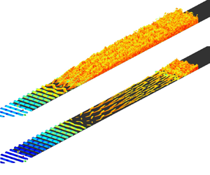
The phase effect on the subharmonic resonance eventually leads to a significant difference in the transition-to-turbulence location, as shown in figure 7. The resonant condition results in staggered  $\varLambda$-shape vortical structures at approximately
  $R=700$ which is the footprint of the subharmonic resonance observed in previous experiments (Corke & Mangano Reference Corke and Mangano1989; Borodulin, Kachanov & Roschektayev Reference Borodulin, Kachanov and Roschektayev2011; Würz et al. Reference Würz, Sartorius, Kloker, Borodulin, Kachanov and Smorodsky2012b) and high-fidelity computations (Sayadi, Hamman & Moin Reference Sayadi, Hamman and Moin2013; Jee et al. Reference Jee, Joo and Lin2018; Kim et al. Reference Kim, Lim, Kim, Jee, Park and Park2019, Reference Kim, Lim, Kim, Jee and Park2020). Fully turbulent flow starts roughly after
  $R=750$ in the resonant condition. In contrast, the anti-resonant condition leads to significantly delayed transition. Staggered
  $\varLambda$-shape vortical structures appear in the long range
  $750 \lesssim R \lesssim 950$ with prolonged structures near the end of the transition. The vortical structures are elongated in the streamwise direction probably because of the weak nonlinear interaction among low-amplitude instabilities expected; see figure 5(c).

Figure 7. Vortical structures in the LES computations with the resonant phase  $\Delta \phi _{in} = 105^{\circ }$ (a) and the anti-resonant phase
  $\Delta \phi _{in} = 10^{\circ }$ (b). The iso-surface of the Q-criteria
  $Q=3 \tilde {U}_\infty ^2 / \tilde {x}^2(R=400)$ is used for the visualisation with the colour contour of the magnitude of the spanwise velocity
  $|w|$.
The skin friction  $C_f$ in figure 8 indicates the transition region affected by the initial phase difference. The resonant conditions (
 $\Delta \phi _{in} = 105$ and
  $130 ^{\circ }$) yield the deviation of
  $C_f$ from the laminar data at approximately
  $R=690$ and the approach to turbulent
  $C_f$ at approximately
  $R=750$. In contrast, the anti-resonant condition with
  $\Delta \phi _{in}=10^{\circ }$ leads to
  $C_f$ deviation from the laminar at approximately
  $R=820$ and the turbulent
  $C_f$ near
  $R=1000$. The prolonged vortical structures in figure 7(b) are associated with the long transition region.

Figure 8. Skin friction  $C_f$ in the current LES computations with various initial phase difference
  $\Delta \phi _{in}$ compared with theoretical data.
Current LES computations indicate that the initial phase difference by itself can control the transition location, which was not disclosed in the literature. The anti-resonant phase delays the turbulent transition location by  $\Delta R \simeq 1000-750 = 250$ which corresponds to
  $\Delta Re_x \simeq 4.4 \times 10^5$, an approximately 80 % increase in the transition Reynolds number from the resonant condition. The phase difference between the fundamental and subharmonic modes was modulated with an array of microphones in previous experiments with non-zero pressure gradient (Borodulin et al. Reference Borodulin, Kachanov and Koptsev2002; Würz et al. Reference Würz, Sartorius, Kloker, Borodulin, Kachanov and Smorodsky2012a). Although complete transition to turbulent flow was not achieved in the experiments of Borodulin et al. (Reference Borodulin, Kachanov and Koptsev2002) and Würz et al. (Reference Würz, Sartorius, Kloker, Borodulin, Kachanov and Smorodsky2012a), the nonlinear interaction was significantly delayed with the anti-resonant phase. The current investigation and the experimental approach in controlling the phase suggest that turbulent transition can be controlled with the phase modulation of a major instability mode (here the subharmonic mode).
3.4. Discussion on resonance and anti-resonance
Resonance and anti-resonance phenomenon of the secondary instability (subharmonic mode) are further discussed here with the evolution of the phase difference between the fundamental and subharmonic modes. A total of 44 initial phases differences are simulated in the current PSE (see figure 4b), and the evolution of four selected phases  $\Delta \phi _{in}=15, 40, 105$ and
  $130 ^{\circ }$ are shown in figure 9. The Floquet analysis is also compared with the PSE data because the Floquet analysis provides the phase-locked condition. Initial phase differences near the Floquet
  $\Delta \phi _{in}$ follow the Floquet phase evolution in the current PSE with a slight deviation at the beginning. As the initial phase difference deviates further from the resonant phase, the phase evolution requires more distance to approach the Floquet phase difference. It takes approximately
  $\Delta R=200$ for the anti-resonant condition of the initial phase
  $\Delta \phi _{in} = 15^{\circ }$ to catch up with the subharmonic resonance, which is consistent with the exponential growth of the subharmonic mode after
  $R\simeq 600$ in figure 4(a).

Figure 9. Evolution of the phase difference between the fundamental 2-D and subharmonic 3-D modes in the current PSE and Floquet analysis with the four selected initial phases.

Figure 10. Evolution of the phase difference between the fundamental 2-D and subharmonic 3-D modes in the current PSE, LES and Floquet analysis with the four selected initial phases.

Figure 11. Comparison of the modal shapes between the current Floquet analysis and PSE computations for anti-resonant conditions. The amplitude is scaled by its own maximum in each case.
The phase evolution is also confirmed in the LES computations as shown in figure 10. Two resonant initial phase differences ( $\Delta \phi _{in}=105$ and
  $130 ^{\circ }$) and two anti-resonant phase differences (
 $\Delta \phi _{in}=10$ and
  $15 ^{\circ }$) are selected for the LES data sets. Two selected PSE cases are also plotted for comparison. In the resonant conditions, the phase difference quickly converges to the Floquet phase difference. For the anti-resonant condition of
  $\Delta \phi _{in}=10 ^{\circ }$ in LES, the phase difference approaches the Floquet data after
  $R=600$, similarly observed in the PSE anti-resonance of
  $\Delta \phi _{in}=15 ^{\circ }$. Note that the anti-resonance phenomena is sensitive to detailed numerical solution, so the difference of
  $5^{\circ }$ seems acceptable, as discussed in § 3.3.
In both PSE and LES, regardless of the initial phase differences,  $\Delta \phi$ converges to the resonant phase difference approximately
  $90^{\circ }$ in the downstream. Similar evolution of the phase difference between two major instability modes (normally primary and secondary instability modes) has been observed in experiments (Borodulin et al. Reference Borodulin, Kachanov and Koptsev2002; Würz et al. Reference Würz, Sartorius, Kloker, Borodulin, Kachanov and Smorodsky2012a). Borodulin et al. (Reference Borodulin, Kachanov and Koptsev2002) noticed a similar convergence to
  $90^{\circ }$ for the phase difference in an adverse-pressure-gradient boundary-layer flow on a flat plate (see Borodulin et al. Reference Borodulin, Kachanov and Koptsev2002, figure 26). The narrow phase range for the anti-resonant condition was also observed in the experiment (see Borodulin et al. Reference Borodulin, Kachanov and Koptsev2002, figure 25). Würz et al. (Reference Würz, Sartorius, Kloker, Borodulin, Kachanov and Smorodsky2012a) also measured the evolution of the phase difference starting from the anti-resonance to the resonance in a boundary layer on a laminar airfoil.
The mechanism of the phase evolution is related to the phase synchronisation of the subharmonic mode for the parametric resonance. A simple dynamic system expressed in Mathieu's equation, which describes a sinusoidal parametric excitation (Kovacic, Rand & Sah Reference Kovacic, Rand and Sah2018), requires the phase synchronisation for the parametric resonance. An initial phase shift of the subharmonic mode eventually approaches to the phase synchronisation (Kim Reference Kim2020), and the transient interval is associated with the initial phase shift. Kim (Reference Kim2020) obtained two opposite local solutions, one for exponential growth (resonance) and another for exponential damping (anti-resonance) in Mathieu's equation. An arbitrary initial condition can be decomposed into these two solutions. Obviously, the resonant component grows exponentially and dominates the subharmonic mode, which results in the phase evolution to the phase synchronisation. A similar discussion can be found in an experimental observation of phase evolution (Borodulin et al. Reference Borodulin, Kachanov and Koptsev2002; Würz et al. Reference Würz, Sartorius, Kloker, Borodulin, Kachanov and Smorodsky2012a).
Initial phase differences in the anti-resonant condition change the mode shape of the subharmonic mode during the transient region towards the phase synchronisation, as shown in figure 11. In the initial damping region  $400 < R < 600$ of the anti-resonant condition, the subharmonic mode undergoes a severe distortion. As the phase difference approaches to the resonant phase predicted by the Floquet analysis at approximately
  $R=600$ (i.e. the phase synchronisation), the subharmonic mode eventually recovers to the resonant shape. In contrast, the resonant condition maintains the initial resonant modal shape as shown in figure 12. Note that the resonant condition is insensitive to the phase shift if the phase difference is in the wide range of
  $60 \lesssim \Delta \phi _{in} \lesssim 150 ^{\circ }$, which has been discussed with figure 4(b).

Figure 12. Comparison of the modal shapes between the current Floquet analysis and PSE computations for resonant conditions. The amplitude is scaled by its own maximum in each case.
The evolution of the temporal oscillation of the fundamental and subharmonic modes shown in figure 13 indicates the variation of the phase speed depending on the initial phase difference  $\Delta \phi _{in}$. The subharmonic oscillation relative to the fundamental oscillation at
  $y_{(1,1),max}$ is plotted in figure 13. The subharmonic mode, initially resonating with the fundamental mode, yields almost no variation in the temporal oscillation, which indicates that the phase speed is synchronised in the overall transition process. In contrast, the anti-resonant initial condition causes the temporal oscillation of the subharmonic mode to continuously shift in the phase until
  $R\simeq 630$. After
  $R>630$, the phase speed of the subharmonic mode remains the same and is synchronised with the phase speed of the fundamental mode, i.e. in the phase synchronisation condition.
3.5. Effect of amplitude on anti-resonance and phase synchronisation
It is well known that the subharmonic resonance is affected by major parameters including the amplitude of the fundamental mode. However, amplitude effects on the evolution of the subharmonic mode, initially in the anti-resonant condition, have not been thoroughly investigated. Particularly, the effect on the phase synchronisation location has not been studied. As a consequence, additional computations with various amplitudes of the fundamental and subharmonic modes are carried out here for the assessment of the amplitude effect on anti-resonance and phase synchronisation. The additional computations are listed in table 2. Due to the computational cost, LES is used for selected cases.
Table 2. Computational cases with various initial amplitudes for the current study of amplitude effects on anti-resonance and phase synchronisation.

The effect of the initial subharmonic amplitude on anti-resonance is shown in figure 14(a). The amplitude evolution of the subharmonic mode is vertically shifted with the initial amplitude of the subharmonic mode itself (see figure 14a). The phase synchronisation location at approximately  $R=630$ remains the same in the LES and PSE computations (see figure 14b), regardless of the initial amplitude of the subharmonic mode in the current study. The subharmonic initial amplitude is sufficiently small compared with the fundamental that the subharmonic amplitude effect on anti-resonance and phase synchronisation is negligible. The growth rates after the phase synchronisation shown in figure 14(a) also confirm that the subharmonic resonance is not significantly affected by the subharmonic amplitude itself. The PSE data show a slight different evolution of the phase difference at approximately
  $R=600$ compared with the LES data, as already discussed in § 3.3 with figure 10.

Figure 13. Temporal oscillation of the fundamental and subharmonic modes during the period of the subharmonic mode  $T_{(1,1)}$ at selected streamwise locations. The LES computations are used: red dashed line,
  $(1,1)$; black solid line,
  $(2,0)$. Each mode amplitude is scaled with its own maximum. (a) Initially resonant condition,
  $\Delta \phi _{in}=105^{\circ }$. (b) Initially anti-resonant condition,
  $\Delta \phi _{in}=10^{\circ }$.

Figure 14. LES and PSE computations with various initial amplitudes of the subharmonic mode  $A_{(1,1)}(x_0)$ and anti-resonant initial phase differences. (a) Amplitude growth. (b) Evolution of phase difference.
The effect of the initial fundamental amplitude on anti-resonance is shown in figure 15. The higher initial fundamental amplitude induces larger growth of the subharmonic mode (see figure 15a) and earlier phase synchronisation (see figure 15b). The subharmonic amplitude quickly grows double exponentially with the highest fundamental amplitude  $2 \times A_{(2,0)}$ owing to the strong driving force of the large fundamental mode. The phase synchronisation occurs at approximately
  $R=500$ with the highest fundamental amplitude in both LES and PSE. The subharmonic mode decays initially in all the cases in figure 15 because of the anti-resonant condition. The decaying rate also depends on the initial amplitude of the fundamental mode, the higher fundamental amplitude leads to more reduction at approximately
  $R=450$ in the subharmonic amplitude. The low amplitude of the fundamental mode in the case of
  $0.1 \times A_{(2,0)}(x_0)$ cannot trigger the subharmonic resonance, and both the fundamental and subharmonic modes decay at approximately
  $R=620$ in the current PSE computation.

Figure 15. LES and PSE computations with various initial amplitudes of the fundamental mode  $A_{(2,0)}(x_0)$ and anti-resonant initial phase differences. (a) Amplitude growth. (b) Evolution of phase difference.
Interestingly, the case of  $A_{(2,0)}$ yields phase synchronisation much delayed compared with the case of
  $0.5 \times A_{(2,0)}$. This is presumably associated with the large distortion of the subharmonic mode in the case of
  $A_{(2,0)}$ compared with the case of
  $0.5\times A_{(2,0)}$ in the region of
  $450 < R < 600$ as shown in figure 16. It is speculated that the large distortion of the mode shape in the case of
  $A_{(2,0)}$ causes a greater distance to recover, which may cause the amplitude to dwindle until approximately
  $R=600$ in figure 15(a).
The effect of the initial fundamental amplitude on the subharmonic resonance with the resonating initial condition is shown in figure 17. Note that the PSE with the highest initial amplitude ends earlier compared with the other cases because these major modes  $(2,0)$ and
  $(1,1)$ are already at 1 % of the free-stream velocity. The behaviour of the subharmonic mode affected by the fundamental amplitude is expected owing to the nature of the parametric resonance.
4. Conclusions
A thorough investigation has been conducted into the phase effect on the growth of a secondary instability in the early nonlinear transition region and its final impact on the turbulent transition location. Numerical methods with various levels of fidelity were systematically explored. The fundamental 2-D TS wave and subharmonic oblique wave were chosen for the primary and corresponding secondary instability, respectively.
Floquet analysis provides a resonating subharmonic mode for a given basic flow composed of steady laminar flow and the fundamental TS wave with the assumption of locally parallel basic flow and a one-way nonlinear effect from the basic flow to the subharmonic mode. The current Floquet analysis was validated against the pioneering analysis of Herbert et al. (Reference Herbert, Bertolotti and Santos1987) and the experimental data of Kachanov & Levchenko (Reference Kachanov and Levchenko1984) for the same flow condition. In such an early nonlinear stage in the laminar region, local Floquet analysis is efficient for obtaining the subharmonic mode resonating to the given basic flow.
Because the current Floquet analysis is limited to a resonating condition, PSE was used for the new parametric study on the effect of the phase on the subharmonic resonance. A total of 44 phase differences between the fundamental and subharmonic modes were studied by shifting the subharmonic phase with respect to the given fundamental TS wave while maintaining the initial amplitude of both the waves at the PSE inlet. The current PSE indicates that the subharmonic resonance is insensitive to the phase difference as long as the phase shift is less than approximately  $45 ^{\circ }$ from the most resonating phase condition. In contrast to the resonance phenomena, the anti-resonant condition damps the subharmonic growth at the beginning and delays the resonance significantly. The anti-resonant condition is sensitive to the phase difference here, only
  $5 ^{\circ }$ difference can cause the subharmonic amplitude to vary with a factor of 10 downstream near
  $R=600$ in the current simulation.
To carry through complete simulations to fully turbulent flows, LES was used for nine selected phase differences (two in the resonant condition and seven near the anti-resonance). The current LES provides the subharmonic resonance observed in the Floquet and PSE analyses in the early nonlinear region, indicating that LES is essentially DNS before highly nonlinear interactions occur. Comparisons between PSE and LES were also made in less-resonating conditions, and the comparison is acceptable even in the anti-resonant condition. A slight difference, approximately  $5 ^{\circ }$ in the anti-resonant phase between PSE and LES, is presumably related to the sensitive nature of the anti-resonance phenomena to detailed flow solutions. The turbulent transition is significantly delayed when the subharmonic resonance is mostly suppressed in the anti-resonant condition. The variation of the transitional Reynolds number can be drastic as
  $\Delta Re_{x, tr} \simeq 4.4\times 10^5$, when the phase shifts from the resonant to anti-resonant condition. Although a realistic transition control technique with the phase modulation requires further investigation, a few experimental approaches with an array of microphones in Borodulin et al. (Reference Borodulin, Kachanov and Koptsev2002) and Würz et al. (Reference Würz, Sartorius, Kloker, Borodulin, Kachanov and Smorodsky2012a) indicate the control potential.
The resonance and anti-resonance phenomenon were further discussed with the evolution of the phase difference. In a resonating condition, the phase difference quickly follows the phase evolution of the Floquet analysis even though the initial phase is moderately deviated from the Floquet phase. In the anti-resonant condition, it takes a significant distance for the subharmonic mode to catch up on the phase evolution of the Floquet analysis. The mechanism of the phase evolution is associated with the phase synchronisation of the subharmonic mode for the parametric resonance. A similar phase evolution towards the resonant phase has been noticed even in a simple nonlinear dynamic system governed by Mathieu's equation (Kim Reference Kim2020) and experimental measurements under non-zero pressure gradients (Borodulin et al. Reference Borodulin, Kachanov and Koptsev2002; Würz et al. Reference Würz, Sartorius, Kloker, Borodulin, Kachanov and Smorodsky2012a). In the anti-resonant condition, the subharmonic mode shape deviates from the resonating shape at the beginning as the subharmonic amplitude damps, and then it returns to the resonating shape as phase synchronisation occurs.
Because an anti-resonant condition can lead to a significant transition delay, it was imperative to investigate parameters affecting the anti-resonance. Previous studies focused on the parametric resonance of the subharmonic mode in resonant conditions, not anti-resonance. In the current study, amplitude effects on anti-resonance and phase synchronisation were investigated using both the PSE and LES computations. The initial amplitude of the subharmonic mode does not significantly change the evolution of the subharmonic mode in anti-resonant conditions, as long as the subharmonic amplitude is sufficiently small enough not to interfere the one-way influence of the fundamental to subharmonic modes. In contrast, the initial amplitude of the fundamental mode strongly affects the evolution of the subharmonic mode even in anti-resonance and eventually the phase synchronisation location for the subharmonic resonance, the higher fundamental amplitude causes earlier recovery of the subharmonic mode from a desynchronised to a synchronised phase.

Figure 16. Evolution of the subharmonic mode shape from the PSE computations with various initial amplitudes of the fundamental mode and anti-resonant initial phase difference. The amplitude is scaled by its own maximum in each case.

Figure 17. PSE computations with various initial amplitudes of the fundamental mode and initially resonant phase difference.
Funding
This work was supported by the National Research Foundation of Korea (NRF) grant funded by the Korea government (MSIT) (Project No. NRF-2021R1A2C1006193) and Space Core Technology Development Program (No. NRF-2017M1A3A3A02016810). Computational resources were supported by the KISTI National Supercomputing Center (Project Numbers: KSC-2020-CRE-0057 and KSC-2018-CRE-0113) with technical support.
Declaration of interests
The authors report no conflict of interest.
Appendix A. Primary and secondary instability (Floquet) analyses
Equations for the primary instability are obtained for the fundamental TS wave, substituting (2.3) and (2.4) into (2.2), and eliminating non-parallel terms, as provided in the Appendix of El-Hady (Reference El-Hady1988),
 $$\begin{gather} \dot{\zeta}_1 = \zeta_2, \end{gather}$$
 $$\begin{gather}\dot{\zeta}_2 = \left\{ \alpha^2 + \textrm{i} R_o (\alpha U_L-\omega) \right \} \zeta_1 + R_o \dot{U}_L \zeta_3 +\textrm{i} \alpha R_o \zeta_4, \end{gather}$$
 $$\begin{gather}\dot{\zeta}_3 ={-}\textrm{i}\alpha \zeta_1, \end{gather}$$
 $$\begin{gather}\dot{\zeta}_4 ={-}\frac{\textrm{i} \alpha \zeta_2}{R_o} - \left\{ \frac{\alpha^2}{R_o} + \textrm{i} (\alpha U_L-\omega) \right\} \zeta_3, \end{gather}$$
where  $\dot {\zeta }=\textrm {d}\zeta /{\textrm {d}y}$. The set of the first-order differential equations with the boundary conditions given in (A2) yields an eigenvalue problem for the eigenvalue
  $\alpha$ and the eigenfunctions
  $\zeta$.
 $$\begin{gather} \zeta_1 =\zeta_3 = 0 \quad \text{at} \ y=0, \end{gather}$$
 $$\begin{gather}\zeta_1,\zeta_3 \to 0 \quad \text{as} \ y \to \infty. \end{gather}$$
 Substituting (2.5) and (2.6) for the basic flow and the disturbance in (2.2), respectively, with  $\{u, v, w, p \}$ being replaced with
  $\{u, v, w, p \}_{1/2}$, and equating the coefficients of
  $\exp (\pm \textrm {i}\theta /2)$ on both sides, the following set of first-order ordinary differential equations for the secondary instability is obtained.
 \begin{align} \dot{\eta}_1 &= \eta_2, \\ \dot{\eta}_2 &= \varGamma\eta_1 + R_o \dot{U}_L \eta_3 + R_o(\gamma + \textrm{i}\alpha_{1/2}) \eta_4 \nonumber\\ &\quad + AR_o(\gamma + \textrm{i}\alpha_{1/2})\zeta_1 \eta_7 + AR_o\zeta_3 \eta_8 + AR_o\zeta_2 \eta_9, \end{align}
 \begin{align} \dot{\eta}_3 &={-}(\gamma + \textrm{i}\alpha_{1/2})\eta_1 -\beta \eta_5, \\ \dot{\eta}_4 &={-}\frac{1}{R_o}[(\gamma + \textrm{i}\alpha_{1/2})\eta_2 + \varGamma\eta_3 + \beta \eta_6] \nonumber\\ &\quad +A(\gamma - \textrm{i}3\alpha_{1/2})\zeta_3 \eta_7 -A[\gamma - \textrm{i}(\alpha+\alpha_{1/2})]\zeta_1\eta_9 +A\beta \zeta_3 \eta_{11}, \end{align}
 \begin{align} \dot{\eta}_5 &= \eta_6, \end{align}
 \begin{align} \dot{\eta}_6 &={-}\beta R_o \eta_4 + \varGamma \eta_5 +AR_o(\gamma - \textrm{i}\alpha_{1/2})\zeta_1 \eta_{11} + AR_o \zeta_3 \eta_{12}, \end{align}
 \begin{align} \dot{\eta}_7 &= \eta_8, \\ \dot{\eta}_8 &= \varGamma \eta_7 + R_o \dot{U}_L \eta_9 + R_o(\gamma - \textrm{i}\alpha_{1/2}) \eta_{10} \nonumber\\ &\quad +AR_o(\gamma - \textrm{i}\alpha_{1/2}) \zeta^*_1 \eta_1+ AR_o \zeta^*_3 \eta_2 + AR_o \zeta^*_2 \eta_3, \end{align}
 \begin{align} \dot{\eta}_9 &={-}(\gamma - \textrm{i}\alpha_{1/2})\eta_7 -\beta \eta_{11}, \\ \dot{\eta}_{10} &={-}\frac{1}{R_o}[(\gamma - \textrm{i}\alpha_{1/2})\eta_8 + \varGamma^* \eta_9 + \beta \eta_{11}] \nonumber\\ & \quad +A(\gamma + \textrm{i}3\alpha_{1/2})\zeta^*_3 \eta_1 -A[\gamma + \textrm{i}(\alpha^*+\alpha_{1/2})]\zeta^*_1\eta_3 +A\beta \zeta^*_3 \eta_5, \end{align}
 \begin{align} \dot{\eta}_{11} &= \eta_{12}, \end{align}
 \begin{align} \dot{\eta}_{12} &={-}\beta R_0 \eta_{10} + \varGamma^* \eta_{11} +AR_o(\gamma + \textrm{i}\alpha_{1/2})\zeta^*_1 \eta_5 + AR_o \zeta^*_3 \eta_6, \end{align}
where  $\varGamma =\alpha _{1/2}^2+\beta ^2-\gamma ^2 - 2\textrm {i}\alpha _{1/2}\gamma + R_o[\gamma U_L+\textrm {i}(\alpha _{1/2} U_L -\omega _{1/2}))]$ and
  $\beta$ is the spanwise wavenumber for the subharmonic wave. Note that the presence of the fundamental TS wave in the basic flow provides the nonlinear interaction between the fundamental and subharmonic modes through all the terms including
  $U$ and
  $V$ in (2.2) (even the square bracket terms). The nonlinear interaction is one-way in the current analysis because only the subharmonic oblique wave is influenced by the fundamental TS wave, not vice versa. In the derivation from (2.2) to (A3), higher subharmonic modes such as
  $\exp (\textrm {i}3\theta /2)$ are ignored.
Note that the current formulation in (2.6) is an extended version of Nayfeh & Masad (Reference Nayfeh and Masad1990, (33)) and El-Hady (Reference El-Hady1988, (14)) in order to cooperate the complex exponent  $\gamma$ later, whereas the real
  $\gamma$ is assumed in Nayfeh & Masad (Reference Nayfeh and Masad1990) and El-Hady (Reference El-Hady1988). Although the current Floquet analysis is able to handle the complex
  $\gamma$, the subharmonic oblique wave perfectly synchronised with the fundamental TS wave, i.e. the real
  $\gamma$, is of interest here. The physical meaning of the function
  $\eta$ is given in table 3 where
  $\gamma$ is real.
Table 3. Physical meaning of function  $\eta$ for indices 1–6 and the relevant additional function when
  $\gamma$ is real.

The set of 12 differential equations (A3) with boundary conditions given in (A4) yields an eigenvalue problem for the eigenvalue  $\gamma$ and the eigenfunction
  $\eta$,
 $$\begin{gather} \eta_1 =\eta_3 =\eta_5 =\eta_7 =\eta_9 =\eta_{11} = 0,\quad \text{at }\ y=0, \end{gather}$$
 $$\begin{gather}\eta_1,\eta_3,\eta_5,\eta_7,\eta_9,\eta_{11} \rightarrow 0,\quad \text{as} \ y \rightarrow \infty. \end{gather}$$
The Blasius solution is used for the laminar flow  $U_L(y)$. Although the Blasius solution is not strictly parallel (i.e.
  $V \neq 0$ and
  $\partial U_L/\partial x \neq 0$), the assumption of locally parallel flow is used for the analysis of both the primary instability (A1) and the secondary subharmonic instability (A3), following the previous approach in Herbert (Reference Herbert1984), Herbert et al. (Reference Herbert, Bertolotti and Santos1987), Nayfeh & Masad (Reference Nayfeh and Masad1990) and El-Hady (Reference El-Hady1988).
The total number of the grid points is 512 in the wall-normal distance of  $200 \tilde {\delta }_r$ with approximately 300 points inside the boundary-layer thickness
  $5 \tilde {\delta }_r$, and the first wall-normal grid size is
  $7\times 10^{-3} \tilde {\delta }_r$. The current wall-normal mesh points are obtained using the mapping from a semi-infinite to a finite domain suggested in Schmid & Henningson (Reference Schmid and Henningson2001, Appendix A.4) as described in (A5).
 \begin{align} \left. \begin{aligned} y_j = c_1 \frac{1+h_j}{c_2-h_j}, \quad h_j = \frac{2j - N}{N}, \quad j=0, 1, \ldots, N, \quad N=512,\\ y_0 = 0, \quad y_{N/2}=\frac{c_1}{c_2} = 3.5, \quad y_N = \frac{c_1}{c_2-1}=200, \quad c_1=\frac{700}{193}, \quad c_2=\frac{196.5}{193} \end{aligned} \right\}. \end{align}
Using the Matlab built-in function polyeig, the eigenvalue problem with (A1) and (A2) is solved for the 2-D TS wave. The same function is used for the Floquet analysis (A3) with the boundary condition (A4) to obtain the subharmonic characteristic exponent  $\gamma$ along with the eigenfunctions
  $\eta$. The function polyeig solves the polynomial eigenvalue problem
  $(\boldsymbol{\mathsf{A}}_0 + \boldsymbol{\mathsf{A}}_1 \lambda + \cdots + \boldsymbol{\mathsf{A}}_n \lambda ^n) \boldsymbol {b} = 0$ where
  $\lambda$ is the eigenvalue,
  $\boldsymbol {b}$ is the eigenvector and
  $\boldsymbol{\mathsf{A}}$ is the given square coefficient matrix (see Higham & Higham Reference Higham and Higham2016, Ch. 9.8). For the current quadratic eigenvalue problems,
  $n=2$.


