2 Model description

The governing equations are the two-dimensional, non-rotating equations of motion for a stratified fluid in the Boussinesq limit. The numerical model used for the computations is the spectral solver flow_solve described in Winters & De la Fuente (Reference Winters and De la Fuente2012), with hyper-viscosity to dissipate subgrid scale motions. We consider a background state characterized by a far upstream flow speed $V_{\infty }$ and stratification $N(z)$ incident on a Gaussian topography

(2.1a,b)$$\begin{eqnarray}h=h_{m}\exp (-y^{2}/\unicode[STIX]{x1D70E}_{y}^{2});\quad h_{m}/\unicode[STIX]{x1D70E}_{y}=1/6.\end{eqnarray}$$

The topography is centred in a domain of width $L_{y}=33\unicode[STIX]{x1D70E}_{y}$ and is incorporated via the immersed boundary set-up discussed in Winters & De la Fuente (Reference Winters and De la Fuente2012), with conditions of free-slip at the obstacle surface. While the obstacle is gently sloping ($h_{m}/\unicode[STIX]{x1D70E}_{y}=1/6$), the numerical model itself is non-hydrostatic. The height of the computational domain is $L_{z}=6h_{m}$ and the density profiles considered are as shown in figure 1(b). In the computations, the density step $\unicode[STIX]{x0394}\unicode[STIX]{x1D70C}_{i}$ over a height $\unicode[STIX]{x1D6FF}_{i}$ is represented using a hyperbolic tangent function as

(2.2)$$\begin{eqnarray}\displaystyle \unicode[STIX]{x1D70C} & = & \displaystyle \unicode[STIX]{x1D70C}_{0}+0.5\unicode[STIX]{x0394}\unicode[STIX]{x1D70C}_{2}\left(\frac{L_{z}-z}{L_{z}-z_{0}}\right)\left[1+\tanh \left(\frac{2(z-z_{0}-\unicode[STIX]{x1D6FF}_{i}/2)}{\unicode[STIX]{x1D6FF}_{i}}\right)\right]\nonumber\\ \displaystyle & & \displaystyle +\,0.5\left(\unicode[STIX]{x0394}\unicode[STIX]{x1D70C}_{2}+\unicode[STIX]{x0394}\unicode[STIX]{x1D70C}_{i}+\left(\frac{z_{0}-z}{z_{0}}\right)\unicode[STIX]{x0394}\unicode[STIX]{x1D70C}_{1}\right)\left[1-\tanh \left(\frac{2(z-z_{0}-\unicode[STIX]{x1D6FF}_{i}/2)}{\unicode[STIX]{x1D6FF}_{i}}\right)\right],\quad\end{eqnarray}$$

so that the bottom of the step is located at $z=z_{0}$. The corresponding stratification profiles are then approximately given by

(2.3)$$\begin{eqnarray}N(z)\approx \left\{\begin{array}{@{}ll@{}}N_{\unicode[STIX]{x1D6FF}_{i}};\quad & |z-z_{0}-\unicode[STIX]{x1D6FF}_{i}/2|\leqslant \unicode[STIX]{x1D6FF}_{i}/2,\\ N_{0};\quad & |z-z_{0}-\unicode[STIX]{x1D6FF}_{i}/2|>\unicode[STIX]{x1D6FF}_{i}/2.\end{array}\right.\end{eqnarray}$$

We fix $Fr=0.16$ and consider strong density steps characterized by the dimensional values $N_{0}=10^{-2}\,\text{s}^{-1}$ and $N_{\unicode[STIX]{x1D6FF}_{i}}=8.6N_{0}=8.6\times 10^{-2}\,\text{s}^{-1}$. In Jagannathan et al. (Reference Jagannathan, Winters and Armi2019), we showed that for a blocking scale $\widetilde{\unicode[STIX]{x1D6FF}}$, the appropriate inner horizontal length scale for the overflow is the half-width of the obstacle at the blocking level $\unicode[STIX]{x1D70E}_{y_{\widetilde{\unicode[STIX]{x1D6FF}}}}$. The smallest vertical length scale is the thickness of the density interface $\unicode[STIX]{x1D6FF}_{i}$ which, in our experiments, is much smaller than the blocking scale $\widetilde{\unicode[STIX]{x1D6FF}}$. To resolve these inner length scales, we choose a grid spacing $\unicode[STIX]{x0394}z\approx \unicode[STIX]{x1D6FF}_{i}/6$ and $\unicode[STIX]{x0394}y\approx \unicode[STIX]{x1D70E}_{y_{\widetilde{\unicode[STIX]{x1D6FF}}}}/10$.

A sponge layer of thickness $L_{z}/4$ is placed at the upper boundary to prevent reflection of vertically propagating waves and the upstream boundary condition evolves slowly through an iterative scheme (Jagannathan et al. Reference Jagannathan, Winters and Armi2019) that accounts for upstream influence of the topography. Arrest of the forward energy cascade due to downstream instabilities and overturns is accomplished by sixth-order hyperviscous and hyperdiffusion operators (Winters & De la Fuente Reference Winters and De la Fuente2012). The flow speed is rapidly accelerated from rest toward its target speed $V_{\infty }$ over approximately ten time steps. We judge the flow to be quasi-steady when, at the blocking location just upstream of the crest, the peak speed in the overflow varies in time by less than 1 % of its mean value.

3 Numerical results

When $Fr\ll 1$, across-crest asymmetry induced by upstream blocking forces a flow response that is characterized by hydraulic control at the crest (cf. Winters Reference Winters2016; Jagannathan et al. Reference Jagannathan, Winters and Armi2019). For the uniformly stratified case depicted in figure 1(a), Winters & Armi (Reference Winters and Armi2014) show that the upstream flow has a parabolic shape above the blocking level, with peak speed given by $1.5N_{0}H/\unicode[STIX]{x03C0}$. Further, the blocking scale is also related to the overflow thickness as $\unicode[STIX]{x1D6FF}=H/8$. The statement of volume flux conservation for the overflow then reads (see also Jagannathan et al. (Reference Jagannathan, Winters and Armi2019))

(3.1)$$\begin{eqnarray}N_{0}H^{2}/\unicode[STIX]{x03C0}=V_{\infty }(h_{m}+7H/8).\end{eqnarray}$$

The unknown thickness $H$ is obtained as the positive root of this equation:

(3.2)$$\begin{eqnarray}H=\frac{{\displaystyle \frac{7\unicode[STIX]{x03C0}V_{\infty }}{8N_{0}}}+\sqrt{\left({\displaystyle \frac{7\unicode[STIX]{x03C0}V_{\infty }}{8N_{0}}}\right)^{2}+{\displaystyle \frac{4\unicode[STIX]{x03C0}V_{\infty }h_{m}}{N_{0}}}}}{2}.\end{eqnarray}$$

Note that $H$ can also be written in terms of $h_{m}$ and $Fr$ as

(3.3)$$\begin{eqnarray}H=\frac{{\displaystyle \frac{7\unicode[STIX]{x03C0}}{8}}h_{m}Fr+h_{m}\sqrt{\left({\displaystyle \frac{7\unicode[STIX]{x03C0}}{8}}\right)^{2}Fr^{2}+4\unicode[STIX]{x03C0}Fr}}{2}.\end{eqnarray}$$

Thus for a fixed $Fr$, the overflow thickness $H$ is directly proportional to $h_{m}$.

Keeping the other parameters same, we now consider the effect of including a strong density step within the stratification profile. In the simulations that follow, we set $Fr=0.16$ and the ratio $N_{\unicode[STIX]{x1D6FF}_{i}}/N_{0}$ to 8.6. Substituting $Fr=0.16$ in (3.2) yields $H=0.96h_{m}$. That is, the bifurcating isopycnal for a uniformly stratified flow at this $Fr$ will be at $z_{op}=h_{m}+(7/8)0.96h_{m}=1.84h_{m}$. When the step is placed at $z_{0}>z_{op}$, we expect to recover the Winters & Armi (Reference Winters and Armi2014) solution, depicted schematically in figure 1(a).

As an example, consider a strong density interface located well above $z_{op}$, at $z_{0}=2.23h_{m}$. Contours of isopycnals and streamwise velocity of the quasi-steady flow for this case (figure 2) reveal that the overflow bifurcates at $z\approx z_{op}$ and not $z=z_{0}$. The vertical profile of the overflow at the upstream blocking location (figure 3) also agrees closely with the parabolic prediction of Winters & Armi (Reference Winters and Armi2014). We also note that the presence of the density step above the bifurcation acts to strongly inhibit isopycnal displacements aloft. This is similar to observations above the Panay Sill by Tessler et al. (Reference Tessler, Gordon, Pratt and Sprintall2010) (e.g. figure 4 of their paper), where the sub-thermocline overflow plunges down the lee slope, but isopycnal displacements above the strongly stratified thermocline are suppressed.

Figure 2. Quasi-steady flow field for 2-D $Fr=0.16$ flow over an infinite ridge with a density step characterized by $N_{\unicode[STIX]{x1D6FF}_{i}}/N_{0}=8.6$ located at $z_{0}=2.23h_{m}$. (a) Isopycnal lines and contours and (b) streamwise velocity contours. Flow is from left to right.

Figure 3. Vertical profile of the steady streamwise velocity at the blocking point $y=-y_{b}$ for $Fr=0.16$ flow over an infinite ridge with a sharp density step located at $z_{0}=2.23h_{m}$. The Winters & Armi (Reference Winters and Armi2014) parabolic overflow prediction is shown in red.

We now present results from two numerical simulations which highlight by comparison the strong coupling between hydraulic control of the overflow and wave excitation aloft. These simulations differ only in the vertical location of the density step, which is now in the height range $h_{m}<z_{0}<z_{op}$, with $Fr$ and $N_{\unicode[STIX]{x1D6FF}_{i}}/N_{0}$ again being set to 0.16 and 8.6, respectively. In the first, we consider a case with the density interface at $z_{0}=1.73h_{m}$. We then lower the interface to $z_{0}=1.33h_{m}$. We will see that a topographically controlled overflow develops in both these flows, but that the flow morphology differs significantly. In particular, the density interface remains nearly flat in one case while it plunges across the crest in the other. We will see that whether the interface plunges with the overflow or not is determined by the fundamental condition for crest control, namely that the upstream flow be subcritical to a long gravity wave mode.

The theoretical construct of a bifurcating isopycnal (Smith Reference Smith1985; Winters & Armi Reference Winters and Armi2014) as depicted in figure 1 has a well-defined bifurcation point, which is the upstream location where the lower branch of the bifurcating isopycnal begins to plunge. In numerical simulations, due to limitations of resolution and instability of the flow downstream (Smith Reference Smith1991; Jagannathan, Winters & Armi Reference Jagannathan, Winters and Armi2017), the bifurcation manifests over a finite region above the blocking location rather than at a single point. This creates some ambiguity in identifying the bifurcating isopycnal. Here, we identify the topmost isopycnal below which the overflow accelerates and plunges across the crest as the bifurcating isopycnal. We will also show by solving the Taylor–Goldstein equation that this is precisely the lowest isopycnal that renders the upstream flow beneath it and above the blocked layer subcritical.

The time averaged, quasi-steady flow field for the case $z_{0}=1.73h_{m}$ (figure 4) exhibits upstream blocking and across-crest asymmetry. An accelerating downslope flow forms beneath a wedge of nearly stagnant mixed fluid, identifiable as the isolating layer. An isopycnal bifurcation occurs just beneath the sharp interface, at $z=z_{0}$, leaving the bulk of the stratified interface above the accelerated layer upstream and above the isolating layer downstream. Directly above the crest, the top of the interface is displaced slightly upward. This appears to be related to the shear instability that develops just downstream of the bifurcation point (e.g. Peltier & Scinocca Reference Peltier and Scinocca1990; Jagannathan et al. Reference Jagannathan, Winters and Armi2017).

3.1 Non-plunging interface: weak perturbations aloft

Figure 4. Same as figure 2 but for $z_{0}=1.73h_{m}$.

The key feature of the flow is that the density interface remains dynamically inactive; that is, it does not plunge across the crest as part of the hydraulically controlled overflow. The flow aloft responds to an effective flat bottom formed by the density interface rather than the real topography below. As a result, only weak flow perturbations occur in this region. These perturbations are small-amplitude, upward-propagating waves excited by time dependent disturbances of the density step near the bifurcation region.

Figure 5. Vertical profile of the steady streamwise velocity at the blocking point $y=-y_{b}$ for $Fr=0.16$ flow over an infinite ridge with a sharp density step located at $z_{0}=1.73h_{m}$. The prediction in red is based on the values of $\widetilde{H}$ and $v_{m}$ from (3.5) and (3.6), respectively. The wave aloft is predicted to have a vertical wavelength $2\unicode[STIX]{x03C0}V_{\infty }/N_{0}$ and perturbation speed amplitude $V_{\infty }N_{0}/N_{\unicode[STIX]{x1D6FF}_{i}}=0.12V_{\infty }$ (see § 6.1), with the phase chosen to match the computed solution.

Figure 5 shows that the overflow profile at the upstream blocking location has a semi-parabolic shape rather than the parabolic shape observed when the stratification is uniform or when the density step is located above $z_{op}$ as in figure 3. Recall that in the Winters & Armi (Reference Winters and Armi2014) solution, the blocking scale is dynamically related to the thickness of the parabolic overflow as $\unicode[STIX]{x1D6FF}=H/8$. Simulations over a range of small $Fr$ suggest that when a strong density step is present at $z=z_{0}<z_{op}$, the dynamical blocking scale is related to the thickness $\widetilde{H}$ of the semi-parabolic overflow as $\widetilde{\unicode[STIX]{x1D6FF}}\approx \widetilde{H}/4$.

The peak speed of the semi-parabolic overflow can be predicted as follows. The volume transport $\widetilde{Q}$ of the overflow must match the far upstream transport below the bifurcating isopycnal, which is simply given by $V_{\infty }z_{0}$ (see figure 1b). The peak speed $v_{m}$ of the overflow at the blocking location is then obtained by solving the volume conservation equation

(3.4)$$\begin{eqnarray}\widetilde{Q}=V_{\infty }z_{0}=(2/3)\widetilde{H}v_{m},\end{eqnarray}$$

with $\widetilde{H}=z_{0}-h_{m}+\widetilde{\unicode[STIX]{x1D6FF}}=z_{0}-h_{m}+\widetilde{H}/4$, yielding

(3.5)$$\begin{eqnarray}\widetilde{H}={\textstyle \frac{4}{3}}(z_{0}-h_{m}).\end{eqnarray}$$

Substituting (3.5) into (3.4), we obtain

(3.6)$$\begin{eqnarray}v_{m}=\frac{9}{8}\frac{V_{\infty }z_{0}}{(z_{0}-h_{m})},\end{eqnarray}$$

which furnishes a complete description of the overflow profile in terms of the known problem parameters $V_{\infty }$, $h_{m}$ and $z_{0}$.

Figure 5 shows that the peak speed of the overflow agrees well with the value obtained from (3.6). Within the density step, the flow speed decreases linearly to the ambient $V_{\infty }$. Finally, above the step, small amplitude oscillations (${\approx}0.15V_{\infty }$) are present. These oscillations are characterized by nearly zero frequency and vertical wavelength identifiable as $2\unicode[STIX]{x03C0}V_{\infty }/N_{0}$, which is consistent with a vertically propagating linear mountain wave. Note that vertical propagation above $z\approx 4h_{m}$ is suppressed by the sponge layer.

3.2 Plunging interface: large amplitude wave aloft

When the density step is located closer to the crest, at $z=1.33h_{m}$, an asymmetric hydraulic response is again observed, but there are important differences with respect to the case $z_{0}=1.73h_{m}$. The isopycnals and streamwise velocity contours of the quasi-steady flow are shown in figure 6. Unlike in the previous case, the upstream flow now bifurcates at the top of the sharp interface, at $z=z_{0}+\unicode[STIX]{x1D6FF}_{i}$. The density step is thus a dynamically active component of the hydraulically controlled plunging overflow. It descends a depth of approximately $\widetilde{H}/2$ from its initial position, which is roughly $1.4V_{\infty }/N_{0}$ for the value $Fr=0.16$ considered.

Figure 6. Same as figure 4 but for $z_{0}=1.33h_{m}$.

Figure 7. Same as figure 5 but for $z_{0}=1.33h_{m}$. The prediction for the peak speed is obtained from (3.8), while the wave aloft is assumed to have a vertical wavelength $2\unicode[STIX]{x03C0}V_{\infty }/N_{0}$ and perturbation speed amplitude of $V_{\infty }$ (see § 6.1). The phase of the wave is chosen to match the computed solution.

The upstream velocity profile again has a semi-parabolic shape (figure 7). To predict its peak speed using a volume flux constraint, equation (3.4) must be modified to include the density step in the overflow. Once again assuming that the velocity decreases linearly within the interface to the ambient $V_{\infty }$, volume flux conservation requires that

(3.7)$$\begin{eqnarray}\widetilde{Q}=V_{\infty }(z_{0}+\unicode[STIX]{x1D6FF}_{i})=(2/3)\widetilde{H}v_{m}+\frac{(v_{m}+V_{\infty })}{2}\unicode[STIX]{x1D6FF}_{i},\end{eqnarray}$$

giving

(3.8)$$\begin{eqnarray}v_{m}=\frac{V_{\infty }(z_{0}+\unicode[STIX]{x1D6FF}_{i}/2)}{(2/3)\widetilde{H}+\unicode[STIX]{x1D6FF}_{i}/2}.\end{eqnarray}$$

Figure 7 shows that the peak speed within the overflowing layer is now well estimated by (3.8). Further, the descending step acts as a virtual topography for the flow aloft and excites a large wave of amplitude approximately $V_{\infty }$ rather than $0.15V_{\infty }$ as in the previous case. Interestingly, a comparison of figure 7 with figure 5 also reveals that there is a phase difference of approximately $\unicode[STIX]{x03C0}$ in the vertical between the mountain wave in the present case and the small amplitude disturbance observed when the interface does not plunge. This is a consequence of the difference in the shapes of the ‘virtual topography’ i.e. the top of the density step in these two flows – it descends sharply past the bifurcation point in one case while rising slightly and subsequently flattening out in the other. A similar ‘virtual topography’ effect on the phase of the flow response aloft was also noted by Armi & Mayr (Reference Armi and Mayr2015) in their comparison of flow over the Sierras with the 1972 Boulder windstorm described by Lilly (Reference Lilly1978).

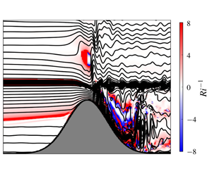
Figure 8 shows snapshots of the inverse Richardson number $Ri^{-1}=(\unicode[STIX]{x2202}v/\unicode[STIX]{x2202}z)^{2}/N^{2}$ for the two cases, where $N$ is the local, instantaneous stratification. Isopycnal overturns in the unstable downslope flow region are visible as patches of negative $Ri^{-1}$. In these simulations, we resolve the formation of the overturns, but the subsequent turbulent dissipation and mixing is modelled using a hyperdiffusive closure scheme. In the plunging interface case, sub-quarter $Ri$ (i.e. $Ri^{-1}>4$) occurs not only downstream, but also upstream and further aloft. As we will describe in § 6, the wave field aloft exhibits large fluctuations in the plunging interface case, suggesting the possibility of instability and nonlinear processes. By contrast, the upstream flow reaches steady state and remains stable despite $Ri$ dropping below $1/4$ in a thin region at the base of the flowing layer.

The emergent picture then is of an intrinsic dynamical connection between hydraulic control of the overflowing layer in direct contact with the topography and the wave field further aloft. The latter is essentially a response to the shape of the virtual topography formed by the top of the density interface and depends sensitively on the dynamics of the hydraulic flow component.

Figure 8. Instantaneous snapshots of the inverse Richardson number overlain with isopycnal contours. (a) Flat interface ($z_{0}=1.73h_{m}$) and (b) plunging interface ($z_{0}=1.33h_{m}$).

4 Theoretical framework – crest control and upstream subcriticality

The underlying basis of the framework we describe is hydraulic control, characterized by subcritical-to-supercritical flow transition at the obstacle crest. A flow profile is defined to be subcritical if it supports at least one long internal wave mode that is able to propagate upstream, supercritical if no such mode exists and critical if the fastest upstream mode is exactly arrested (cf. Pratt et al. Reference Pratt, Johns, Murray and Katsumata1999; Pratt & Whitehead Reference Pratt and Whitehead2007). In the present context, this implies that when the density interface does not plunge, the upstream flow with uniform stratification $N_{0}$ and semi-parabolic velocity profile with peak speed given by (3.6) must be subcritical.

To check for subcriticality, we take the bottom and top of the overflowing layer as rigid boundaries of a waveguide, and solve the Taylor–Goldstein equation to determine whether the predicted upstream flow supports at least one upstream propagating internal wave mode. Assuming a background velocity profile $\bar{V}(z)$, uniform stratification $N_{0}$ and a wave-like disturbance with stream function $\unicode[STIX]{x1D713}=\unicode[STIX]{x1D719}(z)\exp (\text{i}l(y-ct))$, the Taylor–Goldstein equation for a vertical wave mode $\unicode[STIX]{x1D719}(z)$ with speed $c$ is

(4.1)$$\begin{eqnarray}\frac{\text{d}^{2}\unicode[STIX]{x1D719}}{\text{d}z^{2}}-l^{2}\unicode[STIX]{x1D719}+\frac{N_{0}^{2}}{(\bar{V}(z)-c)^{2}}\unicode[STIX]{x1D719}-\frac{1}{(\bar{V}(z)-c)}\frac{\text{d}^{2}\bar{V}(z)}{\text{d}z^{2}}\unicode[STIX]{x1D719}=0,\end{eqnarray}$$

where $u=\text{d}\unicode[STIX]{x1D713}/\text{d}z$ and $w=-\text{d}\unicode[STIX]{x1D713}/\text{d}y$.

For the purpose of this analysis, we redefine the vertical coordinate $z$ so that $z=0$ is the bottom of the overflowing layer. The predicted upstream flow profile has a semi-parabolic velocity distribution

(4.2)$$\begin{eqnarray}\bar{V}(z)=4v_{m}\left(\frac{z}{2\widetilde{H}}-\frac{z^{2}}{4\widetilde{H}^{2}}\right).\end{eqnarray}$$

Bell (Reference Bell1974) showed that in a stratified flow with a sheared velocity profile $\bar{V}(z)$ and stratification $N(z)$ where the Richardson number $Ri$ is greater than $1/4$ everywhere, internal wave modes come in pairs with speeds $c_{j}^{+}$ and $c_{j}^{-}$ such that $c_{j}^{+}>\max (\bar{V}(z))$ and $c_{j}^{-}<\min (\bar{V}(z))$. For $\bar{V}(z)$ given by (4.2), since $\bar{V}(0)=0$, this implies that there always exists an upstream propagating mode provided $Ri>1/4$ everywhere. However, as shown in figure 8(b) for the plunging interface case, $Ri$ drops to sub-quarter values at the base of the flowing layer upstream and so the Taylor–Goldstein equation must be solved to conclusively determine subcriticality.

For the semi-parabolic velocity profile given by (4.2), equation (4.1) can be written as

(4.3)$$\begin{eqnarray}\frac{\text{d}^{2}\unicode[STIX]{x1D719}}{\text{d}z^{2}}-l^{2}\unicode[STIX]{x1D719}+\frac{N_{0}^{2}}{v_{m}^{2}\left[4\left({\displaystyle \frac{z}{2\widetilde{H}}}-{\displaystyle \frac{z^{2}}{4\widetilde{H}^{2}}}\right)-{\displaystyle \frac{c}{v_{m}}}\right]^{2}}\unicode[STIX]{x1D719}+\frac{2}{\widetilde{H}^{2}\left[4\left({\displaystyle \frac{z}{2\widetilde{H}}}-{\displaystyle \frac{z^{2}}{4\widetilde{H}^{2}}}\right)-{\displaystyle \frac{c}{v_{m}}}\right]}\unicode[STIX]{x1D719}=0,\end{eqnarray}$$

with boundary conditions $\unicode[STIX]{x1D719}=0$ at $z=0,\widetilde{H}$. We now non-dimensionalize $z$ as

(4.4)$$\begin{eqnarray}\widehat{z}=z/\widetilde{H}\end{eqnarray}$$

and confine attention to the fastest, long internal wave modes with $l\rightarrow 0$ that diagnose the criticality of the flow. Equation (4.3) then becomes

(4.5)$$\begin{eqnarray}\frac{1}{\widetilde{H}^{2}}\frac{\text{d}^{2}\unicode[STIX]{x1D719}}{\text{d}\widehat{z}^{2}}+\frac{N_{0}^{2}}{v_{m}^{2}\left[4\left({\displaystyle \frac{\widehat{z}}{2}}-{\displaystyle \frac{\widehat{z}^{2}}{4}}\right)-{\displaystyle \frac{c}{v_{m}}}\right]^{2}}\unicode[STIX]{x1D719}+\frac{2}{\widetilde{H}^{2}\left[4\left({\displaystyle \frac{\widehat{z}}{2}}-{\displaystyle \frac{\widehat{z}^{2}}{4}}\right)-{\displaystyle \frac{c}{v_{m}}}\right]}\unicode[STIX]{x1D719}=0,\end{eqnarray}$$

with the boundary conditions $\unicode[STIX]{x1D719}=0$ at $\widehat{z}=0,1$. Strictly speaking, while the base of the flowing layer intersects the topography and may thus be treated as a rigid boundary, the upper boundary is not a true rigid surface, but rather a pliant boundary that can move with the wave. When the fluid overlying the waveguide is stagnant and homogeneous, it is straightforward to impose matching pliant conditions at this boundary (e.g. Smith Reference Smith1991). This is because the solution of (4.1) within the stagnant, homogeneous region takes a particularly simple form of exponential decay. In the flows considered here, the fluid overlying the upstream flowing layer is also stratified, so the formulation of a pliant boundary condition is less obvious. Here we have assumed simple rigid lid conditions at both vertical boundaries.

We now show that the criticality of the flow is completely determined by the two non-dimensional parameters $Fr$ and the ratio $z_{0}/h_{m}$. First, we claim that for any $\unicode[STIX]{x1D6FE}>0$, equation (4.5) is invariant to the following transformation:

(4.6a-c)$$\begin{eqnarray}h_{m}\rightarrow \unicode[STIX]{x1D6FE}h_{m},\quad z_{0}\rightarrow \unicode[STIX]{x1D6FE}z_{0},\quad N_{0}\rightarrow N_{0}/\unicode[STIX]{x1D6FE}.\end{eqnarray}$$

To see this, note that the transformation keeps the control parameter $Fr$ and ratio $z_{0}/h_{m}$ fixed. From (3.5) and (3.6), this leads to a re-scaling of the thickness of the semi-parabolic overflow $\widetilde{H}\rightarrow \unicode[STIX]{x1D6FE}\widetilde{H}$, while $v_{m}$ stays the same. Substituting these re-scaled quantities in (4.5) leaves it unmodified, which shows that the subcritical or supercritical character of the flow is insensitive to this transformation. We remark that this invariance property of (4.5) will not hold but for the long wave approximation $l\rightarrow 0$ that causes the second term in (4.3) to drop out.

If instead, we make the transformation

(4.7a-c)$$\begin{eqnarray}h_{m}\rightarrow \unicode[STIX]{x1D6FE}h_{m};\quad z_{0}\rightarrow \unicode[STIX]{x1D6FE}z_{0};\quad V_{\infty }\rightarrow \unicode[STIX]{x1D6FE}V_{\infty },\end{eqnarray}$$

then $Fr$ and $z_{0}/h_{m}$ are once again unchanged, but (4.5) now becomes

(4.8)$$\begin{eqnarray}\frac{1}{\widetilde{H}^{2}}\frac{\text{d}^{2}\unicode[STIX]{x1D719}}{\text{d}\widehat{z}^{2}}+\frac{N_{0}^{2}}{v_{m}^{2}\left[4\left({\displaystyle \frac{\widehat{z}}{2}}-{\displaystyle \frac{\widehat{z}^{2}}{4}}\right)-{\displaystyle \frac{\widehat{c}}{v_{m}}}\right]^{2}}\unicode[STIX]{x1D719}+\frac{2}{\widetilde{H}^{2}\left[4\left({\displaystyle \frac{\widehat{z}}{2}}-{\displaystyle \frac{\widehat{z}^{2}}{4}}\right)-{\displaystyle \frac{\widehat{c}}{v_{m}}}\right]}\unicode[STIX]{x1D719}=0,\end{eqnarray}$$

where $\widehat{c}=c/\unicode[STIX]{x1D6FE}$. In other words, the eigenvalues of the rescaled problem differ from those of the original one by a factor of $\unicode[STIX]{x1D6FE}$. However, the crucial point is that (4.8) has a negative eigenvalue if and only if (4.5) has one.

Thus only changes to $Fr$ and $z_{0}/h_{m}$ can affect the criticality of the flow. It follows that, for a fixed $Fr$, the criticality of the flow can only be altered by varying $z_{0}/h_{m}$. Based on the results from our numerical simulations, we hypothesize that for a given small $Fr$, there exists $\unicode[STIX]{x1D6FC}>1$ and a corresponding $z_{critical}=\unicode[STIX]{x1D6FC}h_{m}$ such that for $z_{critical}<z_{0}<z_{op}$, the waveguide formed by the semi-parabolic flow profile is subcritical.

Table 1 presents the speed $\min (c_{j}^{-})$ of the fastest upstream propagating internal wave mode within the waveguide formed by this predicted upstream flow for different values of $z_{0}/h_{m}$ at $Fr=0.16$. The wave speeds were computed using the pseudo-spectral generalized eigenvalue solver described in Jagannathan et al. (Reference Jagannathan, Winters and Armi2017). The second and third columns list the wave speeds for a waveguide that excludes and contains the sharp density interface, respectively.

Table 1. Speed of the fastest upstream propagating internal wave mode ($\min (c_{j}^{-})/V_{\infty }$) within the waveguide formed by the semi-parabolic overflow for different locations of the density step at $Fr=0.16$.

When the bottom $z=z_{0}$ of the interface is below $z=z_{op}=1.84h_{m}$ but above a height $1.33h_{m}$ from the ground, the predicted semi-parabolic upstream flow is subcritical. For $z_{0}=1.73h_{m}$, table 1 shows that $\min (c_{j}^{-})=-0.64V_{\infty }$. Thus the bifurcating isopycnal is predicted to lie at the base of the density step. This prediction is consistent with the asymmetric crest-controlled flow observed in the numerical simulation for this case (figure 4).

At $1.33h_{m}$, which we identify as $z_{critical}$, this profile becomes supercritical, which is in violation of the hydraulic control assumption. To resolve this inconsistency, we first note that shifting the upper boundary of the waveguide to include the density interface will increase the mean stratification of the waveguide and thus allow faster upstream propagating waves. Therefore a plausible way to maintain subcriticality is to require that the density interface be part of the controlled overflow. That is, the isopycnal bifurcation occurs at the top rather than base of the density step. The third column of table 1 reveals that for $z=z_{critical}$, the upstream flow indeed becomes subcritical when the density interface is considered to be part of the waveguide. The flow profiles used in performing the wave speed computations for this case are shown in figure 9. The computed flow solution for this case (figure 6) corroborates the waveguide analysis, viz. the top of the density step plunges across the crest as part of the overflow.

Figure 9. Prediction of vertical profiles of the velocity and density within the overflowing layer at the blocking location $y=-y_{b}$ for the case $z_{0}=1.33h_{m}$, with $N_{\unicode[STIX]{x1D6FF}_{i}}/N_{0}=8.6$. Note that the vertical coordinate $z$ has been redefined so that $z=0$ is the base of the flowing layer. Panel (a) excludes the density interface, whereas (b) includes the density interface.

When $z_{0}<z_{critical}$, the semi-parabolic prediction fails to be subcritical even when the interface is considered to be part of the waveguide. Based on the low $Ri$ values observed in figure 8(b) at the base of the flowing layer upstream, it is likely that $z_{critical}$ is near the margin of stability for the semi-parabolic flow configuration. Indeed, simulations for cases with $z_{0}<z_{critical}$ indicate that, while the overflow continues to be asymmetric and hydraulically controlled, its shape and thickness progressively deviate from the predictions here as $z_{0}$ moves further and further below $z_{critical}$. The upstream flow in these cases appears to maintain subcriticality through an upward shifting of the bifurcating isopycnal, to some intermediate height between $z_{0}+\unicode[STIX]{x1D6FF}_{i}$ and $z_{op}$. That is, in addition to the density interface, a portion of the overlying fluid also plunges across the crest as part of the hydraulically controlled overflow.

5 Pressure drag

The pressure drag is a useful diagnostic to characterize the degree of cross-crest asymmetry in flow across topography. It is defined as the decelerating force exerted on the flow by the obstacle,

(5.1)$$\begin{eqnarray}F_{D}=\int _{-\infty }^{\infty }\int _{-\infty }^{\infty }p_{s}\frac{\unicode[STIX]{x2202}h}{\unicode[STIX]{x2202}y}\,\text{d}y\,\text{d}x=\int _{-\infty }^{\infty }\int _{-\infty }^{\infty }h\frac{\unicode[STIX]{x2202}p_{s}}{\unicode[STIX]{x2202}y}\,\text{d}y\,\text{d}x,\end{eqnarray}$$

where $p_{s}$ is the pressure on the obstacle surface. The dynamical significance of pressure drag is that it removes horizontal momentum from the large scale flow and must thus be parameterized in general circulation models of the ocean and atmosphere which do not resolve flow details in the vicinity of topography. For a 2-D obstacle, it is appropriate to consider the drag force per unit length:

(5.2)$$\begin{eqnarray}F_{D}=\int _{-\infty }^{\infty }p_{s}\frac{\unicode[STIX]{x2202}h}{\unicode[STIX]{x2202}y}\,\text{d}y=\int _{-\infty }^{\infty }h\frac{\unicode[STIX]{x2202}p_{s}}{\unicode[STIX]{x2202}y}\,\text{d}y.\end{eqnarray}$$

As Winters & Armi (Reference Winters and Armi2014) show, in blocked downslope flows, there is a continuous drop in surface pressure starting at the upstream blocking location. It is this pressure drop that accelerates the lowest isopycnal of the overflowing layer up and across the crest. Consequently, there arise large surface pressure anomalies between the upstream and downstream sides, which will produce a high drag force on the obstacle. Figure 10 shows the evolution of the normalized drag per unit length as a function of non-dimensional time $t_{\unicode[STIX]{x1D6FF}}^{\prime }=t/t_{\unicode[STIX]{x1D6FF}}$ for the flat and plunging interface simulations. Here $t_{\unicode[STIX]{x1D6FF}}=V_{\infty }/\unicode[STIX]{x1D70E}_{y_{\unicode[STIX]{x1D6FF}}}$ is a time scale for the development of the overflow (Jagannathan et al. Reference Jagannathan, Winters and Armi2019) and $\unicode[STIX]{x1D70E}_{y_{\unicode[STIX]{x1D6FF}}}$ is the half-width of the ridge at the blocking level. The drag has been normalized with the force produced due to a 2-D hydrostatic linear mountain wave excited by a ridge of identical shape and height, and for the same values of the outer flow parameters, $F_{DL}=\unicode[STIX]{x1D70C}_{0}V_{\infty }N_{0}h_{m}^{2}$ (see appendix A).

Figure 10. Evolution of the normalized pressure drag force. The dotted line represents the finite ridge case considered in Jagannathan et al. (Reference Jagannathan, Winters and Armi2019) in which flow splitting leads to reduced drag.

Both the flat and plunging interface flows gradually evolve to a high-drag state. After $t_{\unicode[STIX]{x1D6FF}}^{\prime }\approx 30$, the relative amplification of the drag in the flat interface simulation has a mean value of around 3.25. In the plunging interface flow, a further reduction of the surface hydrostatic pressure occurs along the lee slope and the non-dimensional drag reaches a value of approximately 3.75 at late times. In other words, the pressure drag is approximately 15 % higher when the interface plunges. It is pertinent to consider that in realistic low $Fr$ geophysical flows, lateral flow splitting will often mitigate the surface pressure anomaly across the topography. To illustrate this, we have also shown in figure 10 (dotted lines) the drag for uniformly stratified flow past a long but finite ridge, with cross- to along-stream length ratio $30$ at the same $Fr=0.16$ – a flow that was investigated in Jagannathan et al. (Reference Jagannathan, Winters and Armi2019). At early times, the non-dimensional drag across this ridge approaches 1.5, but over a longer time scale, it drops to around half the linear value, consistent with the fact that flow splitting is a low-drag process compared to mountain wave excitation.

Under the assumption that the drag is dominated by the blocked response, Klymak, Legg & Pinkel (Reference Klymak, Legg and Pinkel2010) used a two and a half layer model to predict its value in 2-D flows where $Fr\ll 1$. When the total water depth $L_{z}\gg h_{m}$, this can be written in our notation as

(5.3)$$\begin{eqnarray}F_{D_{2.5}}=\unicode[STIX]{x1D70C}_{0}V_{\infty }N_{0}h_{m}^{2}\frac{\unicode[STIX]{x03C0}}{2}(1+\unicode[STIX]{x03C0}Fr-2\unicode[STIX]{x03C0}^{2}Fr^{2}).\end{eqnarray}$$

From their 2-D simulations, Klymak et al. (Reference Klymak, Legg and Pinkel2010) report that (5.3) approximates the drag quite well for very low values of $Fr$ ($Fr\sim O(10^{-2})$). For the value $Fr=0.16$ considered here (5.3) yields $F_{D_{2.5}}\approx 1.57\unicode[STIX]{x1D70C}_{0}V_{\infty }N_{0}h_{m}^{2}$ which is an underprediction by a factor of 2 even in the ‘flat-interface’ case (figure 10). This is likely because (5.3) does not take into account the dynamics in the lee, in particular flow instabilities in the moderately low $Fr$ flows considered here that lead to the formation of a deep, nearly stagnant and homogeneous isolating layer downstream (e.g. figure 4). The isolating layer causes a further drop in the lee surface pressure and thus an increase in the pressure drag.

6 The wave field aloft

Figure 11. Evolution of the normalized wave energy density above the overflow, within the domain $(y,z)\in [-\unicode[STIX]{x1D70E}_{y},\unicode[STIX]{x1D70E}_{y}]\times [2h_{m},4h_{m}]$.

A robust measure of the wave activity aloft is provided by considering the perturbation wave energy averaged over an appropriately defined area. The perturbation wave energy is the sum of its kinetic and potential energy contributions (KE and PE, respectively),

(6.1)$$\begin{eqnarray}E(y,z,t)=\underbrace{{\textstyle \frac{1}{2}}[(v-V_{\infty })^{2}+w^{2}]}_{KE}+\underbrace{{\textstyle \frac{1}{2}}N^{2}\unicode[STIX]{x1D709}^{2}}_{PE},\end{eqnarray}$$

where $N(z)$ is the background stratification and $\unicode[STIX]{x1D709}(y,z,t)$ is the instantaneous isopycnal displacement at $(y,z)$. For an obstacle with small aspect ratio $h_{m}/\unicode[STIX]{x1D70E}_{y}\ll 1$, the wave activity is largely confined to the region above the obstacle. We thus define the wave energy density $\langle E(t)\rangle$ as the area average over the domain $(y,z)\in [-\unicode[STIX]{x1D70E}_{y},\unicode[STIX]{x1D70E}_{y}]\times [2h_{m},4h_{m}]$. The normalized $\langle E(t)\rangle$ (figure 11) shows that at later times, the mean wave energy density in the plunging interface flow ($z_{0}=1.33h_{m}$) is over six times larger compared to the flat interface case ($z_{0}=1.73h_{m}$). Figure 11 also displays $\langle E(t)\rangle$ for simulations over a range of intermediate values of $z_{0}/h_{m}$. For $z_{0}/h_{m}>1.4$, $\langle E(t)\rangle$ is found to be small, indicating that the interface remains mostly flat. In the range $1.4\leqslant z_{0}/h_{m}<1.33$, $\langle E(t)\rangle$ becomes oscillatory and its mean value grows steadily as $z_{0}/h_{m}$ decreases towards 1.33. This suggests that the interface does not remain completely flat, rather a portion of it plunges. A complete dynamical description of these ‘split interface’ flows is beyond the scope of the present study.

There are large oscillations with time in the wave energy density when the interface plunges ($z_{0}=1.33h_{m}$), revealing a fluctuating nonlinear wave field aloft. This unsteadiness could be due partly to shear instability of the mean mountain wave solution itself, as suggested by the presence of a region aloft where $Ri$ drops below $1/4$ (figure 8b). In addition, perturbations at the top of the unstable plunging flow also propagate vertically and may interact with the mean mountain wave field. To further analyse the fluctuating wave field, we write the flow variables as the sum of time mean and eddy components,

(6.2a)$$\begin{eqnarray}\displaystyle & \displaystyle v=V_{\infty }+\overline{v}(y,z)+v^{\prime }(y,z,t), & \displaystyle\end{eqnarray}$$

(6.2b)$$\begin{eqnarray}\displaystyle & \displaystyle w=\overline{w}(y,z)+w^{\prime }(y,z,t), & \displaystyle\end{eqnarray}$$

(6.2c)$$\begin{eqnarray}\displaystyle & \displaystyle p=p_{0}(z)+\overline{p}(y,z)+p^{\prime }(y,z,t), & \displaystyle\end{eqnarray}$$

(6.2d)$$\begin{eqnarray}\displaystyle & \displaystyle b=b_{0}(z)+\overline{b}(y,z)+b^{\prime }(y,z,t), & \displaystyle\end{eqnarray}$$

$b=-g\unicode[STIX]{x1D70C}/\unicode[STIX]{x1D70C}_{0}$

$(1/\unicode[STIX]{x1D70C}_{0})\unicode[STIX]{x2202}p_{0}/\unicode[STIX]{x2202}z=b_{0}$

$VRS=-\overline{v^{\prime }w^{\prime }}\,\overline{\unicode[STIX]{x2202}v/\unicode[STIX]{x2202}z}$

$HRS=-\overline{v^{\prime }v^{\prime }}\,\overline{\unicode[STIX]{x2202}v/\unicode[STIX]{x2202}y}$

$VBF=\overline{b^{\prime }w^{\prime }}$

The contributions of each of these terms to EKE production are displayed in figure 12 for the plunging interface case ($z_{0}=1.33h_{m}$). Time averages were taken over 50 snapshots, at a sampling rate of $0.5/t_{\unicode[STIX]{x1D6FF}}$. Downstream of the crest, $VRS$ is of similar magnitude as $HRS$ and both are an order of magnitude larger than $VBF$. This implicates the role of overturning Kelvin–Helmholtz instability (Jagannathan et al. Reference Jagannathan, Winters and Armi2017) in EKE production there. By contrast, further aloft $VBF$ is the dominant term (figure 12c), suggesting that the unsteadiness aloft is a manifestation of continuous, reversible exchange of available potential energy between the mean and fluctuating wave fields.

Figure 12. (Left to right) Normalized vertical Reynolds stress $VRS=-\overline{v^{\prime }w^{\prime }}\overline{\unicode[STIX]{x2202}v/\unicode[STIX]{x2202}z}$, horizontal Reynolds stress $HRS=-\overline{v^{\prime }v^{\prime }}\overline{\unicode[STIX]{x2202}v/\unicode[STIX]{x2202}y}$ and vertical buoyancy flux $VBF=\overline{b^{\prime }w^{\prime }}$ contributions to the EKE production for the plunging interface case ($z_{0}=1.33h_{m}$).

The energy equation for internal waves can be written as (e.g. Gill Reference Gill1982; Nash, Alford & Kunze Reference Nash, Alford and Kunze2005)

(6.3)$$\begin{eqnarray}\frac{\unicode[STIX]{x2202}E}{\unicode[STIX]{x2202}t}+\unicode[STIX]{x1D735}\boldsymbol{\cdot }(E\boldsymbol{u})+\unicode[STIX]{x1D735}\boldsymbol{\cdot }(p\boldsymbol{u})=-\unicode[STIX]{x1D716},\end{eqnarray}$$

where $\boldsymbol{u}$ is the velocity vector, $\unicode[STIX]{x1D735}$ the gradient operator and $\unicode[STIX]{x1D716}$ the rate of energy dissipation, in this case, due to hyperviscosity.

We define integral, time mean energy fluxes

(6.4a)$$\begin{eqnarray}\displaystyle & \displaystyle VEF=\langle \overline{Ew+pw}\rangle =\int _{-\unicode[STIX]{x1D70E}_{y}}^{\unicode[STIX]{x1D70E}_{y}}\overline{Ew+pw}\,\text{d}y, & \displaystyle\end{eqnarray}$$

(6.4b)$$\begin{eqnarray}\displaystyle & \displaystyle HEF=\langle \overline{E(v-V_{\infty })+p(v-V_{\infty })}\rangle =\int _{2h_{m}}^{4h_{m}}\overline{E(v-V_{\infty })+p(v-V_{\infty })}\,\text{d}z, & \displaystyle\end{eqnarray}$$

$VEF$

$\overline{pw}$

$\overline{Ew}$

(6.5)$$\begin{eqnarray}\langle \overline{pw}\rangle =\langle \bar{p}\bar{w}\rangle +\langle \overline{p^{\prime }w^{\prime }}\rangle .\end{eqnarray}$$

For a linear mountain wave in an unbounded atmosphere, the direction of the group velocity is vertically upward and tilted upstream. The vertical energy flux then remains constant with height (Eliassen & Palm Reference Eliassen and Palm1961), with nonlinear advection $\overline{Ew}$ being negligible. Figure 13(a) shows that between $z=2h_{m}$ and $4h_{m}$, $VEF$ is on average, approximately three times larger when the interface plunges. The pressure work $\overline{pw}$ and nonlinear advection $\overline{Ew}$ (not shown separately) are found to be of similar order and further, the wave energy flux also includes a significant eddy component (figure 13b). Horizontal flux and dissipative losses account for the net decrease in $VEF$ between $z=2h_{m}$ and $4h_{m}$. Interestingly, even in the case when the interface remains approximately flat and therefore only produces a weak wave response aloft, $VEF$ and $\overline{p^{\prime }w^{\prime }}$ exhibit non-negligible divergences in the vertical, particularly between $z_{0}/h_{m}=2$ and 2.5. These likely arise due to interactions between the mean wave field and time-dependent vertically propagating disturbances excited downstream of the bifurcation region where the flow is unstable. Above $z\approx 4h_{m}$, the waves are strongly damped due to the presence of the sponge layer.

Figure 13. Vertical energy fluxes as defined in (6.5) for the flat ($z_{0}=1.73h_{m}$) and plunging ($z_{0}=1.33h_{m}$) interface cases: (a) total flux including nonlinear energy advection. (b) Eddy component due to the pressure work term.

7 Summary and conclusions

The presence of a density step in the stratification profile can have a profound effect on the dynamics of fluid flow over topography. In this study we have demonstrated that, in low $Fr$ blocked flows, a sharp density step above crest level can set the height of the isopycnal bifurcation and thereby influence both the nature of the hydraulically controlled overflow as well as the flow response further aloft.

The observations of Armi & Mayr (Reference Armi and Mayr2015) showed that when a neutrally stratified layer is capped by a temperature inversion, i.e. a stable density step, the flow aloft responds to the virtual topography formed by the inversion layer. They found that, depending on the ambient conditions, the overflow may be subcritical, supercritical or hydraulically controlled and asymmetric across the crest. The exact nature of the overflow and the corresponding shape of the inversion across the crest were then shown to be well described using single-layer reduced-gravity hydraulics.

Unlike the Armi & Mayr (Reference Armi and Mayr2015) study and the earlier works of Vosper (Reference Vosper2004) and Jiang (Reference Jiang2014), in the present study, we consider a lower layer which is sufficiently stratified for blocking effects to be significant. In these flows, the natural across-crest asymmetry induced by upstream blocking triggers a hydraulic response, regardless of the location of the step. This differs from the study of Vosper (Reference Vosper2004) in which the formation of a hydraulic plunging flow depends sensitively on the inversion strength and location. The reduced gravity shallow water theory of Jiang (Reference Jiang2014) is also rendered inapplicable when upstream blocking occurs. On the other hand, the hydraulic framework outlined here can successfully interpret the nature of the crest-controlled overflow and in particular predict whether the density interface will plunge across the crest. We find that a plunging density interface can give rise to a wave field aloft that is as much as six times more energetic and produces 15 % higher pressure drag compared to a non-plunging interface. In general the relative amplification of the wave energy density and drag will depend on the ratio $N_{\unicode[STIX]{x1D6FF}_{i}}/N_{0}$.

In uniformly stratified, blocked, topographically controlled flows that feature a sharp density step, a one-way decoupling exists in the sense that the hydraulically controlled flow in contact with the topography is isolated from the flow further aloft. The energetics of the wave field aloft, however, depend sensitively on the dynamics of the controlled flow component. The top of the density step constitutes a ‘virtual topography’ for the flow above and whether or not it participates in the overflow is shown to be directly connected to the fundamental condition of maintaining a subcritical flow upstream. A hydraulic waveguide analysis correctly diagnoses the shape of the density interface across the crest. When the interface plunges across the crest, it produces a highly energetic wave field aloft. By contrast, when the interface remains flat, wave excitation is strongly suppressed. In general, a quantification of the topographically controlled flow component is essential to determine the shape of the virtual topography and hence to predict the characteristics of the flow response further aloft.