


1. Introduction
1.1. Vortex reconnection: relevance and previous work
Three-dimensional viscous vortex reconnection has been a topic of strong interest for the fluid mechanics community over the past several decades due to its important role in a wide variety of flows. In the wake of large aircrafts, for example, pairs of anti-parallel lift-induced vortices spontaneously reconfigure into arrays of vortex rings via viscous reconnection, through a process known as Crow instability (Crow Reference Crow1970). Such aircraft trailing vortices can pose a considerable hazard to other aircrafts (Olsen, Goldburg & Rogers Reference Olsen, Goldburg and Rogers1970; Spalart Reference Spalart1998). Vortex reconnection (Hussain Reference Hussain1986) and pairing (Petersen, Kaplan & Laufer Reference Petersen, Kaplan and Laufer1974; Zaman & Hussain Reference Zaman and Hussain1980) have also been investigated as possible mechanisms for aerodynamic noise generation. Vortex reconnection also plays a key role in fine-scale turbulent mixing (Hussain Reference Hussain1986) and in sustaining the turbulent energy cascade (Hussain & Duraisamy Reference Hussain and Duraisamy2011).
Pioneering works in vortex reconnection include the experimental studies by Fohl & Turner (Reference Fohl and Turner1975), Schatzle (Reference Schatzle1987) and Oshima & Izutsu (Reference Oshima and Izutsu1988) on colliding vortex rings. Early numerical studies mainly focused on three simple configurations: vortex rings (Ashurst & Meiron Reference Ashurst and Meiron1987; Kida, Takaoka & Hussain Reference Kida, Takaoka and Hussain1989; Aref & Zawadzki Reference Aref and Zawadzki1991); perturbed anti-parallel vortices (Pumir & Kerr Reference Pumir and Kerr1987; Melander & Hussain Reference Melander and Hussain1988; Kerr & Hussain Reference Kerr and Hussain1989); and orthogonal vortices (Zabusky & Melander Reference Zabusky and Melander1989; Zabusky et al. Reference Zabusky, Boratav, Pelz, Gao, Silver and Cooper1991; Boratav, Pelz & Zabusky Reference Boratav, Pelz and Zabusky1992). However, the circulation-based Reynolds number considered in these early studies was confined to the range  $Re_\varGamma = 1000\text {--}3500$ due to limitations in computational resources required to capture the small vortical scales involved in the vortex reconnection process. Another crucial parameter determining the cost of these computations is the thickness of the initial vortex core relative to the box size (if Cartesian computational domains are used) and to a characteristic length scale of the vortex (for example, total vortex length or mean radius for a torus knot, and so on).
More recent contributions have investigated viscous reconnection at higher Reynolds numbers. Moet et al. (Reference Moet, Laporte, Chevalier and Poinsot2005) conducted large-eddy simulations (LES) at  $Re_{\varGamma }=10^7$ focusing on the formation of axial flow, i.e. flow velocity oriented along the vortex centreline or axis, in a study of Crow instability. Hussain & Duraisamy (Reference Hussain and Duraisamy2011) presented results up to
  $Re_{\varGamma }=9000$ and observed the so-called cascaded reconnection, i.e. successive reconnections of secondary structures. Van Rees, Hussain & Koumoutsakos (Reference Van Rees, Hussain and Koumoutsakos2012) performed simulations up to
  $Re_{\varGamma }=10\,000$ and revealed the dynamics of first and second reconnection of anti-parallel vortices, with and without imposed axial flow. In the latest work (Yao & Hussain Reference Yao and Hussain2020b), with a similar anti-parallel configuration, the Reynolds number range has been extended up to 40 000. These simulations are all focused on a simple vorticity set-up (i.e. anti-parallel vortices) with a relatively thick core (radius of vortex core to shortest domain length ratio
  $r_e/L \sim 0.1$). In contrast, the study presented in this paper features a large box size and thin core (
 $r_e/L \approx 0.0045$). The computational challenge for vortex dynamics simulation is not only given by Reynolds number, also its multi-scale nature is provided by the disparity in length scale between the coherent structure, the domain box size and vortex-core size. This is a great addition to the computational challenge to this paper.
1.2. Knotted vortices: viscous reconnection and helicity dynamics
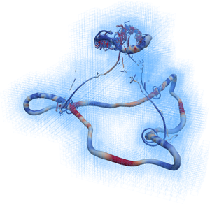
The present study focuses on a thin core, topologically non-trivial vortex set-up – a trefoil knot (figure 1), which, due to its geometrical complexity, features viscous reconnection involving both anti-parallel vortex tubes, as well as the linkage and knottedness of vortices during their topological evolution, which is also of special interest to the quantum fluid dynamics community (see Barenghi Reference Barenghi2007; Maucher, Gardiner & Hughes Reference Maucher, Gardiner and Hughes2016). The first simulations of knotted vortices in viscous flow were conducted by Kida & Takaoka (Reference Kida and Takaoka1987, Reference Kida and Takaoka1988), who first identified a new reconnection mechanism termed bridging. Knotted vortex dynamics in viscous flows did not raise more interest until the work of Kleckner & Irvine (Reference Kleckner and Irvine2013), which was the first experimental study of knotted vortices in viscous fluids. They observed an initial stretching of the vortex line, as well as the topological alteration of the vortex structure and generation of two separate vortex rings after reconnection. Using a similar set-up, Scheeler et al. (Reference Scheeler, Kleckner, Proment, Kindlmann and Irvine2014) observed that the centreline helicity should be conserved during the topological change from a single trefoil vortex to two separate vortex rings under thin-core assumption. Yet Kimura & Moffatt (Reference Kimura and Moffatt2014) predicted that vortex-tube-integrated helicity should decay, using a low-order model based on Burgers vortices. The most recent numerical work by Kerr (Reference Kerr2018a) studies a strongly perturbed thick-core trefoil knot featuring only one reconnection (instead of three, that would occur in absence of perturbations), and focuses on the scaling of the time to first reconnection, enstrophy and circulation for  $Re_{\varGamma }=250\text {--}16\,000$ with the ratio between core radius and mean radius
  $\bar {R}/r_e$ of 5 and 10. In contrast, the present article presents an unperturbed trefoil knot set-up with thin vortex core (
 $\bar {R}/r_e=16.875$), demonstrating that reconnection yields a significant rise in global helicity, that is, domain-integrated helicity, due to small-scale turbulent production events, which intensify as
  $Re_\varGamma$ increases. In the present work a canonical trefoil knot set-up with thin vortex core is considered, and, compared with previous studies, the emphasis is placed on the study of the generation of small scales during the reconnection process and their role in the increase of global helicity levels, the intensity of which is driven by
  $Re_\varGamma$.

Figure 1. Initial vortex shape defined via the parametric equation (2.1), where  $r_e$ is the initial effective vortex-core radius;
  $R_{min}$ and
  $R_{max}$ the minimum and maximum knot radius. The knot half-thickness (in the
  $z$ direction) is taken as equal to
  $R_{min}$. The trefoil vortex propagates in the
  $+z$ direction due to the self-induced velocity field.
1.3. Computational cost, adaptive mesh and subgrid-scale modelling
Knotted vortex simulations present two main computational challenges. The first comes from the requirement to resolve the topologically complex vortex knot with enough points in its viscous core. This constraint is independent of the circulation-based Reynolds number, which alone is not a sufficient metric for assessing the cost. The necessity of (1) accurately resolving the vortex cores and (2) using a sufficiently large domain to limit the influence of the computational boundaries poses serious resolution problems for approaches based on Cartesian grids. In the latter case, the ratio between the (initial) effective vortex-core radius,  $r_e$, and the computational domain size
  $L$, becomes a significant measure of the difficulty to resolve the initial scales. This issue has led previous work on reconnection at high Reynolds numbers – summarized above – to focus on thicker cores (with respect to the computational domain size) and/or only on a portion of the vortex tube or ring under consideration, i.e. on periodic unit problems.
The second challenge lies in capturing the reconnection process, during which the generated smaller scales and complex topology change need to be resolved, or adequately modelled via subgrid-scale (SGS) closures if turbulence is indeed present. The key metric here is Reynolds number which determines the extent of the range of scales created during the reconnection. The cost of a direct numerical simulation (DNS) executed on a uniform Cartesian grid is prohibitively expensive, requiring, for example, 8 billion mesh grid points to simulate a knotted vortex at  $Re_{\varGamma }=4000$ (Kerr Reference Kerr2018a).
These two computational challenges justify the use of an adaptive mesh refinement (AMR) technique, which constitutes a powerful tool that allows to concentrate the grid resolution only where needed, and pick a sufficiently large box size to minimize spurious interactions from the boundaries. Adaptive mesh refinement has been a popular approach in computational fluid dynamics for its capability of capturing multi-scale features with considerable computational savings – at the expense of a considerably more complex code architecture and post-processing strategy. The AMR technique has been extensively employed in many applications: magnetohydrodynamics (Anderson et al. Reference Anderson, Hirschmann, Liebling and Neilsen2006; Dumbser et al. Reference Dumbser, Zanotti, Hidalgo and Balsara2013), incompressible multiphase flows as for the droplet motions in a microchannel (Chen & Yang Reference Chen and Yang2014) and the atomization of liquid impinging jets (Popinet & Rickard Reference Popinet and Rickard2007), compressible multiphase flows as for the leakage of gas from a liquefied-petroleum-gas storage cavern (Pau et al. Reference Pau, Bell, Almgren, Fagnan and Lijewski2012) or for bubble dynamics (Tiwari, Freund & Pantano Reference Tiwari, Freund and Pantano2013), etc. For vortex dynamics problems, the time evolution, reconnections and decays involve highly transient and localized physics, which is particularly suitable to be solved by AMR. Early work of the application of AMR for vortex dynamics simulation found in the literature can be dated to Almgren, Buttke & Colella (Reference Almgren, Buttke and Colella1994), in which AMR is used to solve an incompressible vortex dynamics problem with fast method of local correction. Popinet (Reference Popinet2003) developed an incompressible AMR solver to simulate a vortex merging problem in complex geometries. Benkenida, Bohbot & Jouhaud (Reference Benkenida, Bohbot and Jouhaud2002) compares two refinement strategies: patched grid and AMR in simulating the transport of vortices. Harris, Sheta & Habchi (Reference Harris, Sheta and Habchi2010), Wissink et al. (Reference Wissink, Kamkar, Pulliam, Sitaraman and Sankaran2010), Chaderjian (Reference Chaderjian2012), Chaderjian & Ahmad (Reference Chaderjian and Ahmad2012) developed different numerical methods combined with Cartesian AMR to simulate the vortical flows in the wake region past helicopter rotor blades.
An alternative approach is to use LES, which enables the investigation of the high-Reynolds-number dynamics of such flows, as only the larger energy-carrying structures are resolved while the SGS are modelled. Moreover, if the adopted LES procedure is capable of adequately simulating the dynamics of the integral length scale of the flow regardless of the specific spectral location of the grid cut-off, resolving the initial vortex core would ideally constitute the only computational constraint and accurate results could be obtained even with a very simple approach based on a Cartesian grid. It is in fact of interest to the authors to evaluate how an LES method used on a fixed mesh compares with a fully resolved DNS calculation (necessarily executed) on an AMR framework.
One shortcoming of traditional LES modelling approaches is their tendency to introduce excessive SGS dissipation in transitional regions or to impact the evolution of the large coherent laminar vortices, which may be on the verge of break-up. Smagorinsky's (Reference Smagorinsky1963) model, for example, attenuates velocity gradients at all scales of the flow, resulting in an undesired damping of the kinetic energy carried by the large scales. Thus, the recently developed coherent-vorticity preserving (CvP) eddy viscosity correction by Chapelier, Wasistho & Scalo (Reference Chapelier, Wasistho and Scalo2018), which is able to capture accurately the dynamics of transitional vortical flows with marginal resolution (Chapelier, Wasistho & Scalo Reference Chapelier, Wasistho and Scalo2019), is adopted in the present study.
Further considerations regarding costs and limits on the Reynolds number achievable can be made by looking at previous work focused on anti-parallel vortex reconnection. Moet et al. (Reference Moet, Laporte, Chevalier and Poinsot2005) performed LES with 4.6 million grid points and  $L/r_e=40$; Misaka et al. (Reference Misaka, Holzäpfel, Hennemann, Gerz, Manhart and Schwertfirm2012) conducted LES with 78.6 million grid points with
  $L/r_e=147.7$ at
  $Re_{\varGamma } \sim 10^7$ to simulate anti-parallel vortex pairs with six points inside the vortex core. The DNS by Hussain & Duraisamy (Reference Hussain and Duraisamy2011) adopted 0.26 to 1073 million grid points (yielding from 13 to 200 points inside the core, respectively), with
  $L/r_e=9.4$, spanning the circulation-based Reynolds numbers in the range 250–9000, and Van Rees et al. (Reference Van Rees, Hussain and Koumoutsakos2012) adopted 785 million points, with 130 points inside the core and
  $L/r_e=16.31$, on
  $Re_{\varGamma } = 10^4$ to capture the detailed evolution process. However, none of these studies provided a grid converge analysis.
In the present study, for the highest Reynolds number considered ( $Re_{\varGamma } = 6\times 10^3$), up to 83.78 points per vortex core are used with
  $L/r_e=220$ for DNS with AMR, and up to 7.68 points per vortex core are used with
  $L/r_e\approx 110$ for LES, alongside a careful grid convergence study spanning three levels of grid resolution for each Reynolds number.
1.4. Manuscript outline
The present study introduces the first DNS and a companion LES of the dynamics of thin-core knotted vortices, for Reynolds numbers up to  $Re_{\varGamma }=6000$, while adopting a box size large enough to not vitiate the flow dynamics (see appendix A). A detailed description of the first reconnection is presented and flow visualizations are presented at a later time of evolution capturing the vortex bursting process, featured by converging axial flow, which is in turn excited by the reconnection. Vortex bursting is observed for the first time in the context of this flow; such phenomenon is challenging to observe in experiments since the tracer can fail to track the vortex after bursting, as discussed by Misaka et al. (Reference Misaka, Holzäpfel, Hennemann, Gerz, Manhart and Schwertfirm2012).
The outline of the paper is as follows. Section 2 introduces the governing equations, the CvP-LES methodology, the adopted AMR framework and the flow configuration, followed by a grid convergence and sensitivity study in § 3. Section 4 focuses on the study of flow kinematics and § 5 is devoted to the characterization of flow structures before, during and after reconnection. Section 6 studies how the time evolution of helicity is impacted by the reconnection process.
2. Problem formulation
2.1. Initial condition
The vortex filament of a trefoil knot is described via the parametric curve:
 \begin{equation} \boldsymbol{X}(\theta) = \begin{pmatrix} R_{min}\left(\sin(\theta)+2\sin(2\theta)\right) \\ R_{min}\left(\cos(\theta)-2\cos(2\theta)\right) \\ -R_{min}\sin(3\theta) \end{pmatrix} \end{equation}
with the local knot radius given by
 \begin{equation} R(\theta) = \sqrt{R_{min}^2 \sin ^2(3 \theta)+R_{min}^2(5-4\cos(3\theta)) }. \end{equation}
Here  $R_{min}$ is the minimum radius, and also the knot half-thickness in the propagation direction (figure 1). The mean radius, defined as
 \begin{equation} \bar{R}=\frac{1}{2{\rm \pi}}\int_0^{2{\rm \pi}}R(\theta) \,\textrm{d} \theta, \end{equation}
will be used as a characteristic length scale in the present study, where we also choose the knot half-thickness to be  $R_{min}$, resulting in
  $R_{max}=3R_{min}$,
  $\bar {R}=2.243R_{min}$ or
  $\bar {R}=0.748R_{max}$. All of the geometrical parameters used in the present study are illustrated and summarized in figure 1 and table 1.
Table 1. Geometrical parameters defining the knotted vortex filament and initial effective viscous core radius,  $r_e$.
The velocity field induced by the vortex filament is initialized by numerically integrating the Biot–Savart law:
 \begin{equation} \boldsymbol{u}(\boldsymbol{x})=-\frac{\varGamma}{4{\rm \pi}} \int{K_v\frac{\left(\boldsymbol{x}-\boldsymbol{X}(\theta)\right)\times \boldsymbol{t}(\theta)}{\left|\boldsymbol{x}-\boldsymbol{X}(\theta)\right|^3}\textrm{d}\theta}, \end{equation}
where  $\boldsymbol {t}(\theta )$ is the unit vector tangent to the filament,
  $\varGamma$ is the circulation and
  $K_v$ is a regularization function taken from Vatistas’ vortex-core model (Vatistas, Kozel & Mih Reference Vatistas, Kozel and Mih1991). The expression for
  $K_v$ is proposed by Van Hoydonck, Bakker & Van Tooren (Reference Van Hoydonck, Bakker and Van Tooren2010) for the vortex-core tangential velocity as a function of the radial distance from the core centre:
 \begin{equation} K_v=\frac{\left|\boldsymbol{x}-\boldsymbol{X}(\theta)\right|^3} {{\left(\left|\boldsymbol{x}- \boldsymbol{X}(\theta)\right|^{4}+{r_c}^{4}\right)}^{{3}/{4}}}. \end{equation}
Here  $r_c$ is the nominal vortex tube radius, which we relate to the effective core radius
  $r_e$ via
  $r_e = 2r_c$. With this choice, a vortex tube of diameter
  $2r_e$ accounts for 95 % of the vorticity carried by the tube. With this kernel function choice, a Gaussian profile can be obtained in the initialized vortex-core structure. Core thickness is a very crucial factor affecting the overall dynamics as well as the small scales for this problem. The purpose of this paper is to report the numerical simulation results of the evolution of a thin-core vortex knot, whose thickness is inspired by Irvine's experimental investigations of a knotted vortex (Kleckner & Irvine Reference Kleckner and Irvine2013).
Simulations are performed in a triply periodic cubic domain with dimensions  $\varOmega =[0,L]^3$, with the trefoil knot vortex initialized at the centre (
 $0.5L,0.5L,0.5L$) with
  $L=30R_{min}$ for AMR simulation and
  $L=15R_{min}$ for LES. Appendix A provides the analysis on the sensitivity of the box size, showing that
  $L=15R_{min}$ is a sufficient box size for the current study. All simulations are run with circulation
  $\varGamma =0.02$ m
 $^2$ s
 $^{-1}$ and
  $r_e/ \bar {R}=0.059$ (see table 1).
The circulation is set to  $\varGamma =0.02$ m
 $^2$ s
 $^{-1}$ for all cases and changes in Reynolds number
  $Re_{\varGamma }=\varGamma /\nu$ are achieved by solely changing the viscosity. The ratio of specific heats
  $\gamma =1.4$, reference density
  $\rho _{ref} = 1.0$ and reference temperature
  $T_{{ref}}=1.0$ are used to compute the reference pressure
  $p_{{ref}}=\rho c^2/ \gamma$. In the following text, a non-dimensional time
  $t^*=t\varGamma /\bar {R}^2$ is used to display transient data.
2.2. Governing equations
The flow motion considered is assumed to be governed by the set of compressible Navier–Stokes equations,
 \begin{equation} \mathcal{NS}(\boldsymbol{{w}})=\frac{\partial{\boldsymbol{{w}}}}{\partial{t}}+\boldsymbol{{\nabla}}\boldsymbol{{\cdot}} \left[\boldsymbol{\mathsf{F}}_{{c}}(\boldsymbol{{w}})-\boldsymbol{\mathsf{F}}_{{v}}(\boldsymbol{{w}},\boldsymbol{{\nabla}}\boldsymbol{{w}})\right]=\boldsymbol{{0}}, \end{equation}
where  $\boldsymbol {{w}}=(\rho ,\rho \boldsymbol {{U}},\rho E)^{\mathrm {T}}$ is the vector of conserved variables
  $\rho$,
  $\boldsymbol {{U}}$ and
  $E$, density, velocity and total energy, respectively, and
  $(\boldsymbol {{\nabla }}\boldsymbol {{w}})_{ij} = \partial {w_i}/\partial {x_j}$ its gradient. The viscous and convective flux tensors
  $\boldsymbol {\mathsf {F}}_{{c}},\boldsymbol {\mathsf {F}}_{{v}}\in \mathbb {R}^{5\times 3}$ read as
 \begin{equation} \boldsymbol{\mathsf{F}}_{{c}}=\begin{pmatrix} \rho\boldsymbol{{U}}^{\mathrm{T}}\\ \rho\boldsymbol{{U}}\otimes\boldsymbol{{U}}+ p\boldsymbol{\mathsf{I}}\\ (\rho E+p )\boldsymbol{{U}}^{\mathrm{T}} \end{pmatrix}\quad \mathrm{and}\quad \boldsymbol{\mathsf{F}}_{{v}}=\begin{pmatrix} \boldsymbol{{0}}\\ \boldsymbol{\tau}\\ \boldsymbol{\tau}\cdot\boldsymbol{{U}}-\lambda\boldsymbol{{\nabla}} T^{\mathrm{T}} \end{pmatrix}, \end{equation}
where  $T$ is the temperature,
  $p$ is the pressure,
  $\lambda$ is the thermal conductivity of the fluid and
  $\boldsymbol {\mathsf {I}} \in \mathbb {R}^{3\times 3}$ is the identity matrix. For a Newtonian fluid, we have
 \begin{equation} \boldsymbol{\tau}=2\mu\boldsymbol{\mathsf{S}}, \end{equation}
where  $\mu$ is the dynamic viscosity and
 \begin{equation} \boldsymbol{\mathsf{S}}=\tfrac{1}{2}\left[\boldsymbol{{\nabla}}\boldsymbol{{U}}+\boldsymbol{{\nabla}}\boldsymbol{{U}}^{\mathrm{T}}-\tfrac{2}{3} \left(\boldsymbol{{\nabla}}\boldsymbol{{\cdot}}\boldsymbol{{U}}\right)\boldsymbol{\mathsf{I}}\right].\end{equation}
The ideal gas law is considered for the closure of the system of equations, namely,
 \begin{equation} p=(\gamma-1)\left(\rho E-\tfrac{1}{2}\rho\boldsymbol{{U}}\cdot\boldsymbol{{U}}\right), \end{equation}
where  $\gamma$ is the heat capacity ratio.
2.3. Adaptive mesh refinement computational framework: the VAMPIRE code
The DNS of the knotted vortex reconnection presented in this work are performed with the AMR high-order compact finite difference code VAMPIRE (Zhao & Scalo Reference Zhao and Scalo2020). The AMR framework of the VAMPIRE code is based on Paramesh (MacNeice et al. Reference MacNeice, Olson, Mobarry, De Fainchtein and Packer2000). For each simulation, before time advancement, a sensor estimating the discretization error of the sampled initial condition is ran on all the blocks to determine whether the mesh should be locally refined; such a process is repeated until convergence of the AMR tree structure. A sample of the resulting adaptively refined mesh at time  $t^*=0$, as well as subsequent times, is shown in figure 2 for
  $Re_\varGamma =6000$.

Figure 2. Grid following the vortex transport in the DNS simulation with AMR. The upper row and lower row show different views of the simulation results for  $Re_\varGamma =6000$.
In this work our goal is to apply the AMR code to fully resolve the vortex reconnection dynamics. Therefore, we choose to use a vorticity-based sensor, defined in the non-dimensional form as
 \begin{equation} {f_\omega } = \frac{{ |\boldsymbol{{\nabla}} (\omega )| \varDelta}}{{\max \left( {{{\left\| \omega \right\|}_\infty }, {\omega _{\textrm{{ref}}}}} \right)}}, \end{equation}
where  $\varDelta$ is the local grid spacing, and
  $\omega$ is the magnitude of vorticity, i.e.
  $\omega := |\boldsymbol {\omega }|$. This expression is the normalized gradient of vorticity by a local indicator of the vorticity magnitude. From a numerics perspective to avoid division by zero, an extra term
  $\omega _{{ref}}$ is added to the denominator of the expression.
This reference vorticity value is expected to be a measure for the global level of vorticity magnitude. The sensor is expected to refine the grid in the region where the vortical features are significant, while coarsening the grid at the regions far away from the vortex ring, where the vorticity vanishes. More details of the numerics can be found in Zhao & Scalo (Reference Zhao and Scalo2020). The AMR structure is updated every time step. All of the AMR simulation results presented in this paper are run at  ${CFL}=0.25$.
2.4. Large-eddy simulation framework on Cartesian grid
In the present study, the compressible LES formalism introduced by Lesieur & Metais (Reference Lesieur and Metais1996) and coworkers (Lesieur & Comte Reference Lesieur and Comte2001; Lesieur, Métais & Comte Reference Lesieur, Métais and Comte2005) is adopted yielding the following set of filtered compressible Navier–Stokes equations:
 \begin{equation} \mathcal{NS}(\bar{\boldsymbol{{w}}}) = \boldsymbol{{\nabla}} \boldsymbol{{\cdot}} \boldsymbol{\mathsf{F}}_{{SGS}} (\bar{\boldsymbol{{w}}},\boldsymbol{{\nabla}}\bar{\boldsymbol{{w}}}). \end{equation}
Here  $\bar {\boldsymbol {{w}}}=(\bar {\rho },\bar {\rho }\widetilde {\boldsymbol {{U}}},\bar {\rho }\widetilde {E})^{\mathrm {T}}$ is the vector of filtered conservative variables. The LES equations are obtained by applying a low-pass filter to the Navier–Stokes equations (Leonard Reference Leonard1974). The spatial filtering operator applied to a generic quantity
  $\phi$ reads as
 \begin{equation} \bar{\phi}(\boldsymbol{{x}},t)=g (\boldsymbol{{x}})\star\phi (\boldsymbol{{x}}), \end{equation}
where  $\star$ is the convolution product and
  $g(\boldsymbol {{x}})$ is a filter kernel related to a cutoff length scale
  $\bar {\varDelta }$ in physical space (Sagaut Reference Sagaut2006). The compressible case requires density-weighted (or Favre) filtering operators, defined as
 \begin{equation} \widetilde{\phi}=\frac{\bar{\rho\phi}}{\bar{\rho}}. \end{equation}
 The SGS tensor  $\boldsymbol {\mathsf {F}}_{{SGS}}$ is the result of the filtering operation, it encapsulates the dynamics of the unresolved SGS, and is modelled here using the eddy-viscosity assumption:
 \begin{equation} \boldsymbol{\mathsf{F}}_{{SGS}}(\bar{\boldsymbol{{w}}},\boldsymbol{{\nabla}}\bar{\boldsymbol{{w}}}) =\begin{pmatrix} \boldsymbol{{0}}\\ 2\mu_{t}\bar{\boldsymbol{\mathsf{S}}}\\ -\dfrac{\mu_{t}C_{p}}{Pr_{t}}\boldsymbol{{\nabla}}\widetilde{T}^{\mathrm{T}} \end{pmatrix}. \end{equation}
Here  $\bar {\boldsymbol {\mathsf {S}}}$ is the shear stress tensor computed from (2.9) based on the Favre-filtered velocity
  $\widetilde {\boldsymbol {{U}}}$,
  $Pr_{t}$ is the turbulent Prandtl number, which is set to 0.5 (Erlebacher et al. Reference Erlebacher, Hussaini, Speziale and Zang1992),
  $C_{p}$ is the heat capacity at constant pressure of the fluid and
  $\mu _{t}$ is the eddy viscosity, which depends on the chosen subgrid model.
In the present work, the CvP-Smagorinsky closure is adopted, which yields accurate results for transitional and high-Reynolds-number flows. The LES methodology employs the CvP approach introduced by Chapelier et al. (Reference Chapelier, Wasistho and Scalo2018), which has been validated in the context of transitional helical vortices simulations (Chapelier et al. Reference Chapelier, Wasistho and Scalo2019). The expression for eddy viscosity for this closure reads as
 \begin{equation} \mu_t=\rho f(\sigma) (C_{\mathrm{S}}\bar{\varDelta})^2\sqrt{2S_{ij}S_{ij}}, \end{equation}
where  $C_{\mathrm {S}}=0.172$ is the Smagorinsky constant,
  $\bar {\varDelta }$ is the local (linear) grid size and
  $f(\sigma )$ is the CvP turbulence sensor built from the ratio of the test-filtered to grid-filtered enstrophy,
 \begin{equation} \sigma=\dfrac{\;\;\widehat{\bar{\xi}}\;\;}{\;\;\bar{\xi}\;\;}, \end{equation}
where  $\bar {\xi }= \bar {\boldsymbol {\omega }} \cdot \bar {\boldsymbol {\omega }}/2$. Near-unitary values of such ratio,
  $\sigma \simeq 1$, imply a low degree of local spectral broadening of the flow (for example, in regions of transitional turbulence or coherent laminar vortices) and, hence, result in the local attenuation of SGS dissipation.
The compressible, Favre-filtered Navier–Stokes equations are solved on a simple uniform Cartesian grid using a sixth-order compact-finite-difference scheme solver originally written by Nagarajan, Lele & Ferziger (Reference Nagarajan, Lele and Ferziger2003), under continued development at Purdue University. The solver is based on a staggered grid arrangement, providing superior accuracy and robustness compared with a fully collocated approach (Lele Reference Lele1992). The time integration is performed using a third-order Runge–Kutta scheme.
For the presently considered computations, the speed of sound is arbitrarily selected as  $c_{ref}=5V_{{max}}$, where
  $V_{{max}}$ is the maximum velocity magnitude at the initial condition. The maximum Mach number is achieved during reconnection and it does not exceed 0.25 in all cases simulated. This choice yields near-incompressible flow dynamics. Simulations are initialized with unitary density and temperature fields, equal to the reference values
  $\rho _{ref} = 1.0$ and
  $T_{{ref}}=1.0$. The gas constant is then defined by setting the reference pressure to
  $p_{{ref}}=\rho _{ref} c_{ref}^2/ \gamma$, where
  $\gamma =1.4$ is the ratio of specific heats. Levels of density, temperature and pressure are dimensionless and physically irrelevant, as the compressibility effects on the simulated hydrodynamics are negligible.
3. Grid sensitivity study
3.1. Grid convergence analysis of AMR calculations
A grid sensitivity analysis has been carried out for all Reynolds numbers considered (figure 3, table 2) based on the globally integrated enstrophy
 \begin{equation} \varXi = \iiint_\varOmega{ \xi\,\textrm{d} V}. \end{equation}
This quantity is highly sensitive to small-scale dynamics and a grid-converged enstrophy evolution is therefore indicating that the resolution is sufficient to capture the small scales generated during the reconnection process. We hereafter describe that state of the AMR tree by reporting the block tree depth,  $d$, and number of grid points per block
  $N_b$. Grid configurations used for the two circulation-based Reynolds numbers considered in this paper include 8 and 9 levels with
  $12^3$,
  $18^3$,
  $24^3$,
  $30^3$,
  $36^3$ grid points per block. As observed from the simulation results, with the refinement sensor specified in § 2.3, all the regions containing the vortex core are initially refined to the finest level; therefore, the resolution provided by the grid configuration can be represented by the number of points inside the initial vortex-core diameter (
 $2r_e/\varDelta$). The enstrophy curves from the two finest simulations in figure 3 overlap each other. An AMR grid with 9 refinement levels,
  $12^3$-points and
  $30^3$-points per block provide grid-converged global enstrophy for the
  ${Re}_{\varGamma } = 2000$ and 6000 cases, respectively. Figure 3 shows that, for both Reynolds numbers, starting from the same initial condition, the global enstrophy decreases first due to viscous dissipation. The dissipation rate is relatively stronger for
  ${Re}_{\varGamma } = 2000$. During reconnection, both enstrophy curves increase and reach their peak, followed by a gradual decay. The peak value of global enstrophy for
  ${Re}_{\varGamma } = 6000$ is significantly higher than the
  ${Re}_{\varGamma } = 2000$ case, and even higher than its initial value, in this case due to the production of very small vortical scales during the reconnection. Whether the latter constitutes the occurrence of turbulence in a state of quasi-equilibrium or not, a proper dynamic LES model tasked with simulating such a highly unsteady and inhomogeneous flow should not vitiate the underlying coherent vortex dynamics by adding unnecessary amounts of eddy viscosity.

Figure 3. Grid convergence analysis for AMR simulations:  $Re_{\varGamma }=2000$ (green),
  $Re_{\varGamma }=6000$ (blue), showing the evolution of the resolved volume-integrated enstrophy
  $\varXi$ (or, equivalently, normalized total viscous dissipation,
  $\epsilon$). The results in the plot include the six AMR simulations at
  $Re_{\varGamma }=6000$ and the three AMR simulations for
  $Re_{\varGamma }=2000$ (see table 2) with increasing levels of grid refinement as shown by the arrow.
Table 2. Summary of flow and grid parameters for the (single-mesh-level, i.e.  $d=1$) Cartesian CvP-LES and the AMR runs, executed on
  $d=8$ and
  $d=9$ mesh levels. Here
  $N^3$ indicates the total number of points per AMR block, or in the whole computational domain for the Cartesian LES,
  $2r_e/\varDelta$ is an estimate of the number of grid points per initial effective vortex diameter, and
  $N_{{tot}}$ is the total degrees of freedom for each simulation in the unit of millions. For AMR simulations,
  $N_{{tot}}$ is taken at
  $t^*=3.0$ right after the reconnection.

3.2. Grid sensitivity study for LES with Cartesian grid
A grid sensitivity analysis of the LES computations has been carried out for all Reynolds numbers considered (figure 4, table 2). Computational grids with  $N^3= 120^3,\ 192^3,\ 288^3$ and
  $432^3$ points are considered, corresponding to, respectively, 3.4, 3.5, 5.1 and 7.6 points inside the initial vortex-core diameter (
 $2r_e$). The adequacy of the adopted grid resolution is also assessed by monitoring the level of SGS, or modelled, dissipation (figure 4). Such quantities are not intended to provide a rigorous statistical representation of the state of turbulence (when and if present at all), since the flow is highly inhomogeneous and unsteady. Such quantities will be merely used to infer the sensitivity of the resolved flow to the grid and the robustness of the adopted CvP-LES closure. As discussed in the following, the flow evolution is in fact laminar (albeit highly unsteady) before and after reconnection, with near-equilibrium turbulence occurring only during reconnection and at higher Reynolds numbers (figure 5), posing an important numerical modelling challenge for the CvP-Smagorinsky closure. As indicated in table 2, the CvP LES conducted in this study are computationally inexpensive compared with DNS with AMR; however, as shown in the rest of the paper, the CvP-LES correctly predicts key features of the flow, such as the jump in global helicity discussed in § 6.1, demonstrating its suitability as a predictive tool for high-Reynolds-number vortical flow evolution. Figure 5 also shows the comparison between one-dimensional spectra extracted in the
  $z$ direction from the CvP-LES and AMR simulations. The overlap in the low wavenumber range indicates that the CvP-LES correctly captures the effects of the unresolved small scales onto the resolved large scale despite the highly inhomogeneous and non-equilibrium nature of turbulence in this flow.

Figure 4. Grid sensitivity analysis for LES:  $Re_{\varGamma }=2000$ (green),
  $Re_{\varGamma }=6000$ (blue) showing the evolution of the resolved volume-integrated enstrophy,
  $\varXi$ (a), normalized total dissipation,
  $\epsilon _{total}$ (b), and SGS to total dissipation ratio (c). Grid resolutions considered are the finest three datasets from each simulation: coarse
  $( \cdots )$; intermediate
  $(\textrm {- - -})$; fine
  $(\textrm {------})$ (see data in table 2). Reference data shown in circles (
 $\circ$) are taken from the finest DNS data.

Figure 5. Grid sensitivity analysis for Cartesian CvP-LES (black) and AMR (green/blue) simulations:  $Re_{\varGamma }=2000$ (a),
  $Re_{\varGamma }=6000$ (b) showing the one-dimensional energy spectra in the
  $z$ direction at the time of first reconnection (
 $t_1$) defined as the time when the maximum dissipation is achieved (see figure 2). Grid resolutions considered are the finest three datasets from each simulation: coarse
  $( \cdots )$; intermediate
  $(\textrm {- - -})$; fine
  $(\textrm {------})$ (see data in table 2). Red dotted line shows a reference
  $-$5/3 slope. Here
  $L_z$ is the domain size in
  $z$ direction.
The volume-integrated resolved enstrophy (figure 4a) increases monotonically with Reynolds numbers and grid resolution, as expected. The peak in total dissipation (figure 4b), which comprises the modelled  $\epsilon _{SGS}$ and the resolved, occurring upon reconnection, varies modestly for all grids considered at any given Reynolds number, indicating a healthy response of the CvP-LES closure. Velocity-fluctuation intensity production only occurs upon vortex reconnection, responsible for the generation of small-scale vortical structures (see § 5), where a non-vanishing SGS energy content is detectable even for the lowest
  $Re_{\varGamma }$ at the highest grid resolution available (figure 4c). An acceptable level of grid convergence on the total dissipation before and after reconnection is achieved for both Reynolds numbers, which can be seen from figure 4(c) in the comparison with the grid-converged AMR results. The high levels of subgrid dissipation at the beginning of the computation (
 ${\sim }70\,\%$ of the total dissipation for the coarser grid) can be explained as the CvP model detects marginally resolved initial vortex cores and proceeds to make them smoother by the action of subgrid dissipation. This process does not impact the subsequent total dissipation evolution (
 $t^*>1$) which is remarkably close to the DNS results for both Reynolds numbers considered.
4. Vortex propagation kinematics
In this section the kinematics of vortical motion are first described from visual inspections of the instantaneous flow fields taken from the DNS-AMR data. These instantaneous flow fields are also discussed in the animation by Yu, Chapelier & Scalo (Reference Yu, Chapelier and Scalo2017) showing preliminary CvP-LES data on this problem. The initial knotted vortex propagates along, and rotates about the  $z$-axis (as seen from figure 6), then gradual distortion and elongation of the vortex filament are observed, due to the self-induced convection velocity of the smaller radius portion of the knot (
 $R(\theta )<\bar {R}$) being higher than that of the outer portion (
 $R(\theta )>\bar {R}$). This leads to the stretching of the vortex line (
 $t^*\approx 1.97$) and three simultaneous reconnections of vortex filaments (
 $t^*=2.59$). After this reconnection event, two distinct vortical structures initially triangular in shape are generated, which then evolve following independent dynamics (
 $t^*=3.94$), analysed later.

Figure 6. Visualizations of  $Q$-isosurfaces with
  $Q\bar {R}^4/\varGamma ^2=97$ extracted from
  $Re_\varGamma =6000$ simulation. Here
  $v_a^*$ denotes the dimensionless propagation velocity of the knot before reconnection (
 $t^*<2.5$);
  $v_{b1}^*$ and
  $v_{b2}^*$ denote the small and large rings velocity, respectively, after reconnection.
Figure 7 shows the magnitude of vorticity averaged in the  $x$–
$x$– $y$ plane as a function of
  $z$ and
  $t$, defined as
 \begin{equation} \left\langle \omega ^*\right\rangle_{xy} = \frac{1}{L^2}\int_0^L \int_0^L | \boldsymbol{\omega} ^*|(x,y,z,t)\,{\textrm{d}x}\,{\textrm{d}y},\end{equation}
Figure 7. Plane-averaged vorticity as a function of  $z$ (vortex propagation direction) and
  $t$. The velocities
  $v_a, v_{b1}$ and
  $v_{b2}$ (see figure 6) are calculated via a linear fit of the local maxima of vorticity in the
  $z$–
$z$– $t$ plane. The dashed lines show the results from DNS, and dots are from LES.
where  $\boldsymbol {\omega } ^*=\boldsymbol {\omega } \bar {R}^2/ \varGamma$. Figure 7 provides the locations of the two vortices generated after reconnection, which propagate in the
  $z$ direction with different speeds; the peak of enstrophy (shown in figure 4) happens between
  $t^* = 2.5$ and
  $t^* = 3.0$, which occurs at the beginning of the separation of the knot into two vortex rings. After the separation, the leading smaller vortex ring shows higher propagation velocity than the following larger ring, because of its smaller mean ring radius.
While the vortex kinematics before the reconnection are similar among the different Reynolds numbers investigated, the flow dynamics during the reconnection are strongly affected by viscous forces. The latter are responsible for intense enstrophy production events, which intensify with  $Re_{\varGamma }$.
The propagation velocity of the initial knotted structure,  $v_a$, and of the smaller,
  $v_{b1}$, and larger,
  $v_{b2}$, vortex rings forming after reconnection can be evaluated via the slope in the
  $z$–
$z$– $t$ plane of the local maxima of vorticity magnitude (figure 7). The corresponding non-dimensional expression can be obtained based on the initial circulation
  $\varGamma _0$ and the mean knot radius,
  $\bar {R}$:
 \begin{gather} v_{a}^* =v_a\bar{R}/\varGamma_0, \end{gather}
 \begin{gather}v_{b1}^*=v_{b1}\bar{R}/\varGamma_0, \end{gather}
 \begin{gather}v_{b2}^*=v_{b2}\bar{R}/\varGamma_0. \end{gather}
As shown in table 3, the values of  $v^*_a$ extracted from present calculations are similar between two Reynolds numbers, justifying the use of the inviscid scaling
  $t^*=t\varGamma /\bar {R}^2$ before the first reconnection. This can be explained from the fact that the core size difference caused by the Reynolds number is negligible compared with the length scale of the coherent vortex structure before reconnection, therefore, the thin-core assumption still holds well and its influence is very little on the overall kinematics.
Table 3. Non-dimensional propagation velocity (4.2c) of the vortex structures before and after reconnection from the AMR/DNS and Cartesian LES data.

Dimensionless vortex propagation velocities after reconnection  $v^*_{b1}$,
  $v^*_{b2}$ depend more significantly on viscous scaling parameters, such as viscosity and core size. After reconnection,
  $v_{b1}^*$ and
  $v_{b2}^*$ increase with
  $Re_{\varGamma }$. The smaller vortex ring propagates approximately three times faster than the larger one. This is consistent with the initial maximum radius
  $R_{{max}}$ of the knotted vortex being three times larger than
  $R_{{min}}$. The increase in the self-propagation velocity for the higher Reynolds number in the
  $z$ direction is more significant for the small ring, because the smaller ring has a smaller radius of curvature while retaining a core of a similar diameter. The self-advection velocity of a ring of radius
  $R_0$ can in fact be approximated as
  $\varGamma /4{\rm \pi} R_0 \ln (R_0/r_e)$ and when the ratio
  $R_0/r_e$ gets close to unity, the propagation speed is more sensitive to
  $r_e$.
Although the propagation speed  $v_a$ in the
  $z$ direction is almost Reynolds-number independent before reconnection, the higher Reynolds number case does exhibit an earlier reconnection time. In this paper, the time when the maximum volume-averaged enstrophy is reached,
  $t_1$, is used to identify the reconnection process. From figure 3,
  $t_1=2.90$ for
  ${Re}_{\varGamma }=2000$ while
  $t_1=2.75$ for
  ${Re}_{\varGamma }=6000$. This can be explained by analysing the comparison of the evolution of
  $Q$-isosurfaces for the two Reynolds numbers shown in figure 8(c): starting from the same initially prescribed velocity field, the vortex knot evolves almost identically for the two Reynolds numbers, until the stretched vortex segments reach an anti-parallel configuration, where the effect of the finite core size becomes important. The higher Reynolds number case presents thinner vortex cores which communicate relatively higher induced velocity to the nearby anti-parallel vortex segments, resulting in earlier reconnection. Figure 8(c) shows that the difference in induced velocity of the nearly anti-parallel vortex segments is primarily in the
  $xy$ plane, instead of in the
  $z$ direction.

Figure 8. (a) Evolution of effective core radius  $r_e$ and (b) instantaneous vortex length
  $\ell (t)$ normalized by the initial vortex length
  $\ell _0$ for
  ${Re}_{\varGamma }=2000$ (green) and
  ${Re}_{\varGamma }=6000$ (blue). Regions shaded via vertical bars represent the time intervals when reconnection is happening, which are partly overlapping for the two different Reynolds numbers. Solid lines are used before reconnection;
  $\square$, large ring after reconnection;
  $\triangle$, small ring after reconnection;
  $(\circ )$, sum of small and large ring vortex length after reconnection. (c) Overlapping of
  $Q$-isosurfaces
  $Q\bar {R}^4/\varGamma ^2=323$ from
  ${Re}_{\varGamma }=2000$ and
  ${Re}_{\varGamma }=6000$ at four different non-dimensional times:
  $t^*=0.53$ and
  $t^*=1.58$ are two instances before reconnection;
  $t^*=2.95$ and
  $t^*=2.53$ are the reconnection times for
  ${Re}_{\varGamma }=2000$ and
  ${Re}_{\varGamma }=6000$ cases, respectively.
The effect of Reynolds number (i.e. viscous effect) on the core size evolution is presented in figure 8(a) and on the stretching of the vortex length in figure 8(b). In this study, the vortex centreline is extracted based on eigenmodes of the velocity gradient tensor following an approach similar to Sujudi & Haimes (Reference Sujudi and Haimes1995), and the boundary of the vortex tube is identified by applying a regression fit of the vorticity distribution to a Lamb–Oseen model on a cut plane perpendicular to the vortex line,
 \begin{equation} \omega(\tilde{r}) = \frac{\varGamma}{{\rm \pi} r_c^2 } \exp{\left( -\frac{\tilde{r}^2}{r_c^2} \right)} \end{equation}
with  $\tilde {r}$ being the distance normal to the centreline in the local cross-sectional plane. The effective core radius
  $r_e$ in this work is taken as twice
  $r_c$ in order to effectively cover around 95 % of the vorticity in a vortex tube of diameter
  $2r_e$. As shown in figure 8(a), before the reconnection happens, the core radius for the
  ${Re}_{\varGamma }=2000$ case is about 1.7 times compared with the
  ${Re}_{\varGamma }=6000$ case, which satisfies the scaling law
  $r_e \sim \sqrt {\nu t}$. The finite core size effect on the induced velocity shows up at about
  $t^*=2.2$ where the two vortex length curves peel off from each other, signifying that two vortex segments are getting close to each other more rapidly for the higher Reynolds number case. The vortex stretching occurs much faster in the
  ${Re}_{\varGamma }=6000$ case, resulting in earlier reconnection.
The reconnection process lasts longer at a lower Reynolds number, which can also be linked to the thicker core size at  ${Re}_{\varGamma }=2000$.
It can be seen from figure 8(b) that, despite the difference in reconnection time and the duration of the reconnection, the length of the resulting vortex loop right after reconnection for the small leading ring and large trailing ring is almost identical for both Reynolds numbers. The length of the vortex knot right before the reconnection is larger than the sum of the small and large rings after reconnection: the difference is accounted for by the length of the vortex lines that constitute the thread structure, which will be analysed in § 5.3.
5. Vortex reconnection dynamics
The trefoil vortex knot considered in the present study unknots via three simultaneous reconnection events. For the high-Reynolds-number case, a cascaded reconnection occurs, i.e. a series of successive reconnections of the secondary structures (identified as thread-like vortices analysed in the next section), first discovered by Hussain & Duraisamy (Reference Hussain and Duraisamy2011), who also found that this phenomenon was promoted by higher Reynolds numbers. Because of the rotational symmetry of the knot about the  $z$-axis, the three simultaneous reconnections are identical in absence of initial perturbation patterns breaking such symmetry. The configuration of the vorticity field at the onset of reconnection is determined by the kinematics of the vortex propagation leading up to reconnection itself, as discussed in § 4. Because of the difference in the propagation kinematics between the two Reynolds number cases, the configuration of the vorticity field at the onset of reconnection is also different. Figure 9 shows the centreline of vortex tube at the onset of the reconnection at two different Reynolds numbers. The onset of reconnection in this work is defined as the moment when the distance between anti-parallel vortex lines falls below
  $r_{e}(t)$, where
  $r_{e}(t)$ as a function of time,
  $t$, can be found in figure 8(a). This distance is illustrated by a short dashed line connecting two dots in figure 9; moreover, for the two Reynolds numbers considered, the reconnection occurs at different times as well as at different locations along the knot. The high-Reynolds-number case features reconnections occurring at earlier time and at a lower value of
  $z$. The vortex centreline configuration at such a tipping point is nearly symmetric: as seen from figure 9 and table 4, the angles between the vectors normal to the vortex line and the line connecting two tipping points (
 $\theta _1$ and
  $\theta _2$, defined as inclination angles) being almost equal for both Reynolds number cases. Curvature at the tipping point, as studied by Moffatt & Kimura (Reference Moffatt and Kimura2019), has been considered to influence the dynamics of reconnection. The result from this work shows that the high-Reynolds-number case results in smaller radii of curvature at both tipping points (namely,
  $R_1=7.3$ and
  $R_2=6.5$ mm) compared with the low-Reynolds-number case (
 $R_1=7.8$ and
  $R_2=9.8$ mm), as illustrated in figure 9 and reported in table 4. This is as expected, as in the high-Reynolds-number case the tipping points experience more intense stretching, resulting in a higher local curvature, following the mechanism explained by Moffatt & Kimura (Reference Moffatt and Kimura2019). A slight increase in curvature at tipping points is observed when the pair of tipping points approaches from far field; however, unlike what is seen in Moffatt & Kimura (Reference Moffatt and Kimura2019), when tipping points are getting close enough and the bridging starts, the curvatures are flattened instead of increasing rapidly, and the vortex lines on both sides of the dividing plane tend to be more anti-parallel. This process is depicted in figure 9(b), where the radii of curvature reach a minimum value and then increase as the two vortex tubes approach each other. This is due to the jet flow induced by two newly formed bridges pushing two threads away from each other. Similar phenomenon of the flattening of the curvature at tipping points is also observable in the numerical study of two colliding rings in Yao & Hussain (Reference Yao and Hussain2020a).

Figure 9. (a,c,d) Reconstructed vortex centreline upon reconnection for  $Re_{\varGamma }=2000$ (green) and
  $Re_{\varGamma }=6000$ (blue). The radii of curvature are marked with black arrows, with the local normal vectors as their directions. Red arrows represent the direction of vectors tangential to the vortex lines. The angle between the normal vectors and the line connecting the two tipping points is marked as
  $\theta$. Panels (c,d) are for
  $Re_{\varGamma }=2000$ at
  $t\varGamma /\bar {R}^2=2.528$ and
  $Re_{\varGamma }=6000$ at
  $t\varGamma /\bar {R}^2=2.370$, respectively. (b) Change in radius of curvature at the tipping points before reconnection.
Table 4. Curvatures and tipping point angles right before reconnection (see figure 9) at two different Reynolds numbers.

Asymmetric vorticity patterns are observed at the onset location of reconnection, despite nearly symmetric geometrical arrangement of the vortex lines. This scenario is analysed using a local coordinate system (figure 10) where the coordinate origin is located at the centre of the reconnecting threads, the  $Y'$–
$Y'$– $Z'$ plane approximately defines the dividing plane, and
  $X'$ and
  $Y'$ axes align with the orientations of bridges and threads, respectively. The coordinate system moves as the reconnection progresses, i.e. as the whole knot rotates and spins during the reconnection. As seen from figure 10, the pattern of the vortex tubes on both sides of the
  $Y'$–
$Y'$– $Z'$ plane shows rotational symmetry around the
  $Z'$-axis, instead of being symmetric with respect to the
  $X'$–
$X'$– $Z'$ plane. The upper left (
 $X'<0, Y'>0$) and lower right (
 $X'>0, Y'<0$) parts of the vortex stay horizontal in the
  $X'$–
$X'$– $Y'$ plane, while the lower left (
 $X'<0, Y'<0$) and upper right (
 $X'>0, Y'>0$) parts deflect downwards. On the other hand, the axial flow pulses are concentrated at the lower end (
 $Y'<0$) of the anti-parallel structure, while the upper end (
 $Y'>0$) features a less intense axial flow, as identified in figure 10 by the shading of helicity density, defined as
 \begin{equation} h=\boldsymbol{{u}} \cdot \boldsymbol{{\omega}}. \end{equation}
Figure 10. (a) Local coordinate system at the reconnection location. Panels (b–e) show the different times during reconnection for  $Re_{\varGamma } = 6000$. Panel (b) shows the onset position and (c,d,e) show the vortex structure evolution as reconnection progresses. Isosurfaces are extracted with a vorticity magnitude of
  $\omega = 0.5\varGamma /{\rm \pi} r_{e,0}^2$ coloured by normalized helicity density.
The helicity density is a quantity of interest to detect the presence of axial flow, corresponding to locations with the same vorticity direction but opposite velocity direction.
During the evolution of a knotted vortex, the generation of four characteristic vortical structures can be identified:  $\langle I \rangle$ anti-parallel structures;
  $\langle II \rangle$ hairpin vortices;
  $\langle III \rangle$ thread structures;
  $\langle IV \rangle$ helical modes (also named Kelvin waves). Events leading to the formation of such structures are observed for both Reynolds numbers considered. Figure 11 shows a side-by-side comparison between DNS and LES at each stage of vortical flow evolution mentioned above. In comparison, LES results preserve the evolution of large-scale structure without resolving the fine-scale turbulent structure generated via reconnection. As shown in figure 12, the CvP sensor function
  $f(\sigma )$ is capable of detecting the under-resolved small scales generated during the reconnection process, and applying SGS dissipation only to those regions. As shown in figure 4(c), the total dissipation (resolved plus modelled via CvP) recovers the peak dissipation calculated from the DNS. Before and after reconnection, the CvP-sensor prevents the SGS from spuriously dissipating the coherent vortex structure, by preventing the SGS stress from being applied to the large-scale vortex parts. In this way, the large-scale kinematics of the vortex evolution are well preserved, as seen from the right column of figure 11. Also, the SGS stresses contribute significantly to the dissipation of the helicity occurring during reconnection, allowing us to recover the peak value of helicity decay rate
  $-\textrm {d} H(t)/\textrm {d} t$ predicted by the DNS calculations, shown later in figure 19 and discussed in § 6. In this section the discussion of the physics of the reconnection dynamics will be relying on the DNS results.

Figure 11. Finest DNS/AMR (a,c,e,g) and LES (b,d,f,h) at  $Re_{\varGamma }=6000$ showing
  $Q$-isosurfaces at
  $Q\bar {R}^4/\varGamma ^2=323$ for
  $\langle I \rangle ,\langle II \rangle ,\langle III \rangle$ and 96 for
  $\langle IV \rangle$, coloured by helicity density;
  $\langle I \rangle$: a pair of anti-parallel vortex lines undergoing viscous cancellation;
  $\langle II \rangle$: hairpin vortices are generated along non-reconnected parts of threads and forming bridges;
  $\langle III \rangle$: newly formed threads;
  $\langle IV \rangle$: helical structures are generated.

Figure 12. Sensor function  $f(\sigma )$ used in the CvP-LES closure in (2.16) at two different time instances from a LES at
  $Re_{\varGamma } = 6000$.
Structures  $\langle I \rangle$ and
  $\langle II \rangle$ form simultaneously and participate in the bridging process. The thread structures
  $\langle III \rangle$ connect the large and small vortex rings during the last stages of reconnection, which culminates with the complete separation of the two rings and the corresponding initialization of helical, or Kelvin waves
  $\langle IV \rangle$. The latter, via nonlinear collisions, lead to repeated (in time and space) momentary ruptures (or burstings) of the vortex topological structure.
5.1. Anti-parallel vortex pair  $\langle I \rangle$

Vortex regions undergoing the highest rate of axial stretching align right before reconnection in an anti-parallel fashion (figure 11,  $t^*=2.42$) and viscously interact. The vorticity in the outer layers of the vortex tube undergoes cancellation through viscous diffusion, forming hairpin vortices acting as bridges (figure 11,
  $t^*=2.62$); the small-scale structures left over from the reconnection process, named threads, form weak topological connections with the two newly formed vortex rings (figure 11,
  $t^*=2.81$), and eventually dissipate.
These dynamics are similar to those observed in Crow instability (Crow Reference Crow1970), which is the most studied scenario for anti-parallel vortex reconnection, investigated in the context of contrail vortices behind an aircraft. The difference with respect to the knotted vortex lies in the source of perturbations. The Crow instability is a mutual induction sinusoidal instability through which the two anti-parallel vortices interact. However, in the present study, the reconnection process is triggered by the vortex self-advection and distortion.
5.2. Hairpin vortex formation via bridging $\langle II \rangle$

Figure 13 illustrates the detail of the reconnection process for  $Re_{\varGamma }=2000$ and
  $Re_{\varGamma }=6000$. While the interaction during the anti-parallel reconnection results in a cancellation of the outer layer vorticity, enhancement of the inner layer one (in the points of contact), and thinning of the vortex tubes (structure 1), the remaining vorticity unaffected by the cancellation is responsible for initiating the bridging process (structure 2 at
  $t^*=3.16$), yielding intermediate hairpin vortex structures on the two extremities of the thinning anti-parallel structures – the leading and following extremity, based on the self-propagation direction of the knot (i.e. along
  ${+}z$). Parts of newly formed hairpin vortices merge into structure 3, spanning both the anti-parallel structure and early hairpin vortex (structure 2). With structures 1 and 2 gradually dissipating, structure 3 becomes dominant with a vortex-core thickness comparable to the original structure and ultimately responsible for completing the reconnection process. This type of reconnection was named bridging by Kida & Takaoka (Reference Kida and Takaoka1994), to be distinguished from the vortex cancellation process described in Fohl & Turner (Reference Fohl and Turner1975) and Oshima & Asaka (Reference Oshima and Asaka1977). The various steps involved in this process are clearly visible at
  $Re_{\varGamma }=2000$, while at
  $Re_{\varGamma }=6000$, the reconnection results in the generation of smaller scale structures. The same process occurs on both ends of the anti-parallel structure, resulting in the initialization of axial flow and the travelling of helical structures, or Kelvin waves, on the small and large vortex rings after separation. The curvature of the bridges causes the repulsion from the reconnection zone due to the induced velocity field, which further stretches the threads.

Figure 13. Visualization of the generation of hairpin vortices from  $Q$-isosurfaces at
  $Q\bar {R}^4/\varGamma ^2=96$ for
  ${Re}_{\varGamma }=2000$ and
  ${Re}_{\varGamma }=6000$ from DNS/AMR data, coloured by normalized helicity density; threads created during the bridging process, intermediate hairpin vortex structure the final dominant hairpin structure are illustrated.
5.3. Thread structures $\langle III \rangle$

Threads are generated at the beginning of the reconnection process as shown in figures 14 and 15 and figure 16 at around  $t^*=2.90$ for
  $Re_{\varGamma } = 2000$ and
  $t^*=2.63$ for
  $Re_{\varGamma } = 6000$. The thread structure is the byproduct of the circulation transfer process from one vortex segment to its anti-parallel neighbour, thus, its generation coincides with the formation of the bridge comprising the hairpin vortex. Similarly to the observation reported by Hussain & Duraisamy (Reference Hussain and Duraisamy2011), the two anti-bridges curl back and retract from one another shortly after they are formed. As the threads in between are stretched, the induced velocity by the bridges tend to change the curvature of the threads, further distancing them from one another, which can be noticed especially at the thread-bridge junctions at
  $Re_{\varGamma } = 2000$. For the higher Reynolds number case
  $Re_{\varGamma } = 6000$, the stretching is more intense so that the anti-parallel structure is squeezed into a thinner film and subsequently breaks down into finer scales due to Kelvin–Helmholtz instability. In contrast to the case
  $Re_{\varGamma } = 2000$ where threads are side by side, two major thread structures in
  $Re_{\varGamma } = 6000$ can be identified, one on the top and the other at the bottom, with the thin-film vorticity remaining in between, as shown in figure 15. The majority of the high vorticity is concentrated at the thread on the top only, and at a high Reynolds number features significant subsequent local reconnections (i.e. cascaded reconnection), which results in small-scale vorticity surrounding the thread on the top. The structure of the small-scale vortices generated by this reconnection is similar to the cascaded bridgelet structure discussed by Yao & Hussain (Reference Yao and Hussain2020b) (C-structure in figure 7(e) of the cited paper), in which the mechanism of the cascade reconnection has been outlined for the
  $Re_{\varGamma }=9000$ case. The difference with the current work is that the strain field in the current paper is asymmetric, resulting in a more asymmetric evolution of the bridgelets (as shown on the lower right of figure 13). The reversal of curvature near the thread-bridge junctions at
  $Re_{\varGamma } = 6000$ can also be observed, but it manifests itself in the form of bifurcations of the threads together with the generation of numerous smaller scale structures (as seen in the lower right parts of figure 13).

Figure 14. Isosurfaces of vorticity magnitude at various times during reconnection:  $\omega = 0.3\varGamma /{\rm \pi} r_{e,0}^2$ coloured in transparent grey and
  $\omega = 1.0\varGamma /{\rm \pi} r_{e,0}^2$ coloured by red at
  $Re_{\varGamma } = 2000$.

Figure 15. Isosurfaces of vorticity magnitude at specific time steps during reconnection:  $\omega = 0.5\varGamma /{\rm \pi} r_{e,0}^2$ coloured in transparent grey and
  $\omega = 3.0\varGamma /{\rm \pi} r_{e,0}^2$ coloured by red at
  $Re_{\varGamma } = 6000$.

Figure 16. Visualization of the threads (marked by dashed rectangles) evolution using  $Q$-isosurfaces with
  $Q\bar {R}^4/\varGamma ^2=323$ for
  ${Re}_{\varGamma }=6000$ DNS coloured by normalized pressure fluctuations (structure
  $\langle III \rangle$) in figure 11.
Along with the separation into leading small and trailing large vortex rings, the threads become stretched in the self-propagation direction  $z$. At the same time, the threads begin to diverge along the large vortex ring due to the convection of the flow around and along vortex tubes (
 $t^*=3.80$).
The main vortex ring structure keeps rotating around the  $z$-axis and the longitudinally stretched threads separate into two parts: one part is convected by the triangular-shaped vortex rings, then wraps around the bridges. This part will stay connected to the reconnection points and rotates together with the two separate rings around the
  $z$ direction. The other part loses the original connection to the main vortex ring structures and stays at its old position in the
  $x$–
$x$– $y$ plane, as seen in the dashed boxes at
  $t^*=4.52$ and
  $5.22$. The large vortex ring will rotate across such stagnating threads, which serves as a source of perturbation that excites more helical structures at the outer layers of vortex rings, as discussed in the next section.
Furthermore, additional asymmetric features of the reconnection in this problem include the relative rotation between two bridges, as can be seen in figure 10(c–e). At  $Re_{\varGamma } = 6000$, the lower bridge, which is part of the larger trailing ring after separation, undergoes a torsional displacement with respect to the threads (i.e. with respect to the Y’-axis defined in the moving local coordinate in figure 10), while the upper bridge on the small ring remains nearly orthogonal to the threads through the entire reconnection process, and the vertical film formed by the threads remains straight. In contrast, at
  $Re_{\varGamma } = 2000$ the two side-by-side threads are further distorted by the relative motions between bridges (see figure 10b). This is due to the asymmetric configuration of the vortex tube and the asymmetric and non-uniform distribution of the axial flow packets at the onset of reconnection.
5.4. Helical structures and Kelvin waves $\langle IV \rangle$

The hairpin vortex structures generated after reconnection are responsible for exciting helix-shaped structures (figure 17), corresponding to two Kelvin-wave packets propagating away from the reconnection region, in opposite directions and with opposite handedness. These structures, coloured in the figure by the helicity density (5.1), are advected by the axial flow, which occurs when the flow velocity vector inside a vortex core is aligned with the vortex line, thus, the positive values denote a propagation along the direction of the vorticity vector (vice versa, if negative).

Figure 17.  $Q$-isosurfaces with
  $Q\bar {R}^4/\varGamma ^2=323$ from DNS results at
  $Re_\varGamma =6000$. Panels (a,b) show the axial flow direction before reconnection; (c,d,b) depicts the Kelvin-wave packet generated and colliding on the leading small ring, and (f–i) show the Kelvin-wave packets travelling and colliding on the large vortex ring after reconnection; (h) shows when the Kelvin-wave packets collide on the large vortex ring, an annular structure is formed; (j) shows the centreline axial flow energy spectrum before, during and after the Kelvin-wave collision event happened on the large vortex ring as shown in (g–i), respectively.
The helical structures travelling along each single side of the triangular-shaped vortex ring periodically collide with each other, then continue to travel past one another. Each collision event exhibits features of vortex bursting as defined by Spalart (Reference Spalart1998), who investigated this phenomenon in the context of contrail vortices in airplane wakes. Vortex bursting is also observed in the reconnection of anti-parallel vortex tubes (Crow instability), after which the axial flow is driven away from the reconnection region as observed in Misaka et al. (Reference Misaka, Holzäpfel, Hennemann, Gerz, Manhart and Schwertfirm2012) and Van Rees et al. (Reference Van Rees, Hussain and Koumoutsakos2012).
When the helical structures collide for the first time, the axial velocities cancel each other and form an annular structure (visualized in figure 17(h) by a local cut plane across the vortex ring). Similar structures and associated dynamics were observed and discussed by Melander & Hussain (Reference Melander and Hussain1994). When such an annular structure propagates along the vortex tube, it develops additional twists, which represent higher helical modes. Spalart (Reference Spalart1998) argues that vortex bursting does not compromise the coherent structure if the circulation-preservation principle is respected, and that experimental smoke visualizations cannot properly track the vortical structure during bursting.
In the present study such collisions occur as the helical, or Kelvin, waves are travelling along the vortex loop with nonlinear interactions. From a spectral energy content standpoint, the collision process transfers the energy from low wavenumbers to higher ones. One way to check this effect is to perform a Fourier analysis of the axial flow energy spectrum on one vortex loop, defined as
 \begin{equation} E_{\tilde{w}}(k,t)=\frac{1}{\ell (t)}\int_\ell \rho \tilde{w}^2|_{r=0} \exp({-j2{\rm \pi} k/\ell\tilde{z}})\,\textrm{d}\tilde{z}, \end{equation}
where  $\tilde {z}$ is the position along the axial direction of the vortex line, and the axial flow velocity
  $\tilde {w}(\tilde {z},r,t)$ is defined as
 \begin{equation} \tilde{w}(\tilde{z},r,t) = \boldsymbol{u} \cdot {\tilde{\boldsymbol{z}}}, \end{equation}
where  $\boldsymbol {{\tilde {z}}}$ is the unit tangential vector of the vortex line, which is normal to the local cut plane, and the boundary of the vortex tube cross-sectional area. Figure 17(j) shows the axial flow energy spectrum before, during and after the first three simultaneous Kelvin-wave collisions on the large trailing ring (figure 17g–i), depicting that the energy is suppressed during the collision, and redistributed to a higher wavenumber after the collision. Also the Kelvin waves are dispersing as they propagate and collide, resulting in a homogeneous distribution of wave energy along the vortex loops. On the leading small ring, similar but more intense events occur, because of the smaller size of the ring. The evolution of helical structures on the small ring can also be observed and the positive and negative helicity parts alternate rapidly due to the shorter length allowing propagation. The small scales generated on the two separated vortex rings, and especially on the leading smaller ring (figure 17d–i), are the result of Kelvin-wave collisions (which result in an energy cascade into smaller scales), and the interaction between the main vortex tube and the threads wrapping around it (as explained in § 5.3). A similar phenomenon can be found in Van Rees et al. (Reference Van Rees, Hussain and Koumoutsakos2012), where energy cascade from nonlinear Kelvin-wave interaction, as well as deformation of the vortex lines on the resulting vortex rings after reconnection is observed. The energy cascade from Kelvin waves is conjectured to be different from Kolmogorov cascade and has been widely discussed by Kozik & Svistunov (Reference Kozik and Svistunov2004), Vinen, Tsubota & Mitani (Reference Vinen, Tsubota and Mitani2003) and Yepez et al. (Reference Yepez, Vahala, Vahala and Soe2009) for quantum turbulence and superfluid turbulence. In Van Rees et al. (Reference Van Rees, Hussain and Koumoutsakos2012) the thread structure stays in the colliding plane because of symmetry and does not wrap around the vortex rings, whereas in the current work, the wrapping of the threads around the vortex tube and the resulting interaction (pairing and merging) further deforms the vortex tubes and adds to the complexity of the small scales generated.
Overall, there are similarities between the reconnection dynamics of topologically complex thin-core vortex knots and of a symmetric parallel reconnection as discussed by previous works, such as Hussain & Duraisamy (Reference Hussain and Duraisamy2011), Van Rees et al. (Reference Van Rees, Hussain and Koumoutsakos2012) and Yao & Hussain (Reference Yao and Hussain2020b), etc. An asymmetric knot configuration, however, results in much more complex fine-scale vortex structures and non-trivial global helicity dynamics. Moreover, the asymmetry increases with increased Reynolds number, which can be reflected by the curvature change shown in figure 9.
6. Helicity evolution dynamics
Helicity is related to the topological features of the flow, like the degree of knottedness, and linkage, as discussed by Scheeler et al. (Reference Scheeler, Kleckner, Proment, Kindlmann and Irvine2014). Knotted vortices are of interest for the study of helicity dynamics due to their non-zero initial global (or total) helicity,  $H$, which is determined by the initial filament topology; for a single vortex ring, the initial global helicity is, in fact, zero. Kida & Takaoka (Reference Kida and Takaoka1988) and Kerr (Reference Kerr2018b) investigated the evolution of total helicity for knotted vortices, observing that it is conserved before reconnection. Kida & Takaoka (Reference Kida and Takaoka1988) focused on low Reynolds numbers at
  $Re_\varGamma =320, 800$ and
  $1600$ with effective core size
  $r_e/\bar {R} \approx 0.1$, where a decay of total helicity starting from the reconnection process, and a mitigation of this decay as the Reynolds number increased, were observed.
In this paper we assess here the sensitivity of the total helicity evolution to the Reynolds number with thin initial vortex-core radius  $r_e/\bar {R} \approx 0.06$. We focus our analysis on three quantities derived from the helicity density field (5.1): total helicity,
  $H(t)$ (6.1); centreline helicity,
  $H_C(t)$ (6.2); and vortex-tube-integrated helicity,
  $H_V(t)$ (6.3).
Total helicity  $H(t)$ is integrated across the entire computational domain,
 \begin{equation} H(t)= \iiint^{+\infty}_{-\infty} \boldsymbol{{u}} \cdot \boldsymbol{{\omega}} \,\textrm{d}\varOmega \approx \int_{0}^L {\int_{0}^L {\int_{0}^L { \boldsymbol{u} \cdot \boldsymbol{{\omega}} \,\textrm{d}\varOmega }}} \end{equation}
and it contains information from all the scales in the flow. In the present study vortex reconnection results in topological changes in the flow, which cause changes in the total helicity investigated below.
Centreline helicity  $H_C(t)$ is defined as
 \begin{equation} H_C(t)= \varGamma \oint \tilde{w}|_{\tilde{r}=0}\,\textrm{d}\ell, \end{equation}
which is useful in theoretical analyses assuming infinitesimally thin vortex tubes with confined helicity. This practically accessible form is adopted by Scheeler et al. (Reference Scheeler, Kleckner, Proment, Kindlmann and Irvine2014), where  $d\ell$ is the infinitesimal length of a line element along the loop, and
  $\tilde {w}$ as a function of
  $\tilde {r}$ is the local axial velocity, defined in (5.3)
Scheeler et al. (Reference Scheeler, Kleckner, Proment, Kindlmann and Irvine2014) reports that centreline helicity,  $H_C(t)$, is approximately conserved during reconnection in a viscous flow, which is confirmed by the results in the present study discussed later. In the present study, the fluid velocity
  $u$ used in (6.2) is evaluated at the centreline of the vortex core using a method similar to Sujudi & Haimes (Reference Sujudi and Haimes1995).
Finally, the vortex-tube-integrated helicity is defined as
 \begin{equation} H_V(t)= \iiint_V \boldsymbol{{u}} \cdot \boldsymbol{{\omega}} \,\textrm{d}\varOmega, \end{equation}
where the volume of the vortex ring  $V$ is defined as the region with distance smaller or equal to
  $r_e$ from the vortex core. In the limit of
  $r_e\rightarrow 0$, (6.3) yields (6.2). The vortex-tube-integrated helicity can be seen as an improvement upon (6.2), as it allows us to take into account the inner structure of a finite-thickness vortex core.
6.1. Total helicity
For the two different Reynolds numbers considered in this study, before reconnection, the total helicity is approximately constant with a value  $H/ \varGamma ^2 \approx -3.3$, in good agreement with the results of Kida & Takaoka (Reference Kida and Takaoka1988) and Scheeler et al. (Reference Scheeler, Kleckner, Proment, Kindlmann and Irvine2014) who report values of
  $H/ \varGamma ^2 \approx 3.28$ and
  $H/ \varGamma ^2 \approx 3.26$, respectively. The difference in sign is merely due to a trivial difference in the handedness of the trefoil knot, specifically, a change in the sign of the
  $z$ component in (2.1).
As shown in figure 18, for  $Re_\varGamma =2000$ (laminar reconnection), a maximum in helicity is reached and a steady decay observed after that. For higher Reynolds numbers, where turbulent production occurs, a significant and more abrupt increase in helicity is observed, followed by a steady increase in helicity. Figure 18 also shows the total helicity results from the finest LES. The results indicate that the LES is capable of capturing the trend of changing of total helicity correctly, including the abrupt helicity production during reconnection and the gradual decay or increase after reconnection, even though no specific helicity-preserving SGS model is employed in this work.

Figure 18. Direct numerical simulation and companion LES data for the evolution of volume-integrated, or total, helicity for  $Re_\varGamma =2000$ (green) and
  $Re_\varGamma =6000$ (blue) for the vortex knot configuration considered in the present study. Direct numerical simulation results are shown by solid lines and the finest LES by circles (
 $\circ$).
To further study this peculiar behaviour, the following helicity budgets are considered:
 \begin{equation} \frac{\textrm{d}}{\textrm{d} t}H = \iiint -2\nu \boldsymbol{\omega} \cdot \left({\boldsymbol{\nabla}} \times \boldsymbol{\omega} \right) \textrm{d} \varOmega. \end{equation}
Here  $\boldsymbol {{\omega }} \cdot (\boldsymbol {{\nabla }} \times \boldsymbol {\omega } )$ is the super-helicity density. Just like kinetic energy, the global helicity is a conserved quantity in an inviscid flow. However, viscous effects may entail an increase or decrease of the helicity depending on the right-hand side of (6.4). Figures 19(a) and 19(b) show the total helicity budget at both Reynolds numbers considered in the DNS. The excellent agreement between the independently evaluated left- and right-hand sides of (6.4) indicates that the evolution of global helicity is well resolved in both cases. The closure of the global helicity budgets, in fact, requires all scales of the flow to be properly resolved, especially due to the three nested spatial derivative operations present in the super-helicity term on the right-hand-side of (6.4). In the LES with CvP-Smagorinsky closure, the eddy viscosity
  $\mu _t$ contributes to the viscous helicity dynamics, as shown in the budget equation
 \begin{equation} \frac{\textrm{d}}{\textrm{d} t}H = \underbrace{\iiint -2\nu \boldsymbol{\omega} \cdot \left( \boldsymbol{{\nabla}} \times \boldsymbol{\omega} \right) \textrm{d} \varOmega}_\textrm{resolved helicity dissipation} + \underbrace{\iiint -\frac{2\mu_t}{\rho} \boldsymbol{\omega} \cdot \left( \boldsymbol{{\nabla}} \times \boldsymbol{\omega} \right) \textrm{d} \varOmega}_\textrm{modelled SGS helicity dissipation}, \end{equation}
where the helicity  $H$ is here intended as based on the resolved velocity and vorticity, and
  $\boldsymbol {\omega }$ is the resolved vorticity vector. Figures 19(c) and 19(d) show the total helicity budget for both Reynolds numbers considered in the LES. The SGS contribution to the helicity dissipation adds on to the resolved contribution, allowing the LES to predict a peak in total rate of helicity change
  $\textrm {d} H(t)/\textrm {d} t$ matching reasonably well with the DNS results (figure 18). As opposed to the DNS/AMR results, the helicity budgets from the LES are not exactly numerically closed, due to the very nature of the adopted LES approach, which exhibits a high wavenumber energy build up. Moreover, the staggered grid arrangement entails various interpolation operations which further propagate numerical error, resulting in a loss of accuracy in the direct evaluation of the super-helicity on the right-hand side of (6.5). These numerical errors, however, vanish when refining the grid, and become negligible only once and if DNS levels of grid resolution are achieved. An explicitly filtered LES approach is expected to yield an exact numerical closure of the budgets, and will be considered in future work. The reader is also directed to previous research (Li et al. Reference Li, Meneveau, Chen and Eyink2006) on the suitability of SGS closure in vortex dominated turbulent flows.
The finest LES resolution for the  $Re_\varGamma =2000$ and
  $Re_\varGamma =6000$ cases is 288
 $^3$ and 432
 $^3$, respectively. When the grid resolution of the LES is increased, the relative importance of the resolved viscous contribution to the total helicity dissipation rate increases with respect to the SGS contribution.
Furthermore, it is interesting to investigate the spatial distribution of helicity and helicity production (super-helicity), and their evolution with time. This is depicted in figures 20 and 21 showing the  $z$ direction distribution of helicity and production of helicity density averaged in the
  $xy$ plane, where
  $z$ is the propagation direction of the self-induced motion of vortex knot. The helicity and production of helicity density average in the
  $xy$ plane are defined as
 \begin{equation} \left\langle h ^*\right\rangle_{xy} = \frac{1}{L^2}\int_0^L \int_0^L h(x,y,z,t) \bar{R}^3/\varGamma^2\,{\textrm{d}x}\,{\textrm{d}y} \end{equation}
and
 \begin{equation} \left\langle \textrm{d} h^*/\textrm{d} t^* \right\rangle_{xy} = \frac{1}{L^2}\int_0^L \int_0^L -2\nu \boldsymbol{\omega} \cdot \left( {\boldsymbol{\nabla}} \times \boldsymbol{\omega} \right) \bar{R}^5/\varGamma^3 \,{\textrm{d}x}\,{\textrm{d}y},\end{equation}
respectively. Figure 20 shows that when the trefoil knot reaches reconnection, the trailing part, which becomes the larger trailing ring, carries the majority of the helicity; on the other hand, the leading part, that becomes the leading smaller ring later, carries almost zero helicity. From figure 17(b), it can be seen that the leading part presents a nearly triangular shape with a distribution of helicity with a nearly zero average. Figure 21 shows that the location of the abrupt helicity increase during the reconnection (reflected in figure 18) at the reconnection regions between the leading and trailing rings. After reconnection, for both the  $Re_{\varGamma }=2000$ and
  $Re_{\varGamma }=6000$ case, the helicity decay is found to be occurring mainly on the large trailing ring (see figure 21). This decay is likely due to the competing effects of Kelvin-wave collision and viscous dissipation.

Figure 19. Global helicity budget at different Reynolds numbers from the DNS and finest LES available: (a)  $Re_{\varGamma }=2000$ DNS, in green; (b)
  $Re_{\varGamma }=6000$ DNS, in blue; (c)
  $Re_{\varGamma }=2000$ LES, in green; (d)
  $Re_{\varGamma }=6000$ LES, in blue. The symbols correspond to:
  $(\circ )$ resolved helicity production term (first term on the right-hand side of (6.4) and (6.5));
  $(\triangle )$ SGS helicity production term (second term in (6.5));
  $(\textrm {------})$ time derivative of resolved global helicity
  $H(t)$ (left-hand side of (6.4) or (6.5)) obtained by differentiating the time series of
  $H(t)$ collected at every Navier–Stokes time step.

Figure 20. Plane-averaged helicity as a function of  $z$ (vortex propagation direction) and
  $t$. The white dashed lines show the positions of vortex rings estimated by the planed-averaged vorticity magnitude, with velocities
  $v_a, v_{b1}$ and
  $v_{b2}$ defined in figure 6 and calculated the same way as in figure 7. The DNS and LES results are compared for each Reynolds number.

Figure 21. Plane-averaged helicity production  $\textrm {d} h^*/\textrm {d} t^*$ as a function of
  $z$ (vortex propagation direction) and
  $t$ from the DNS results. The white dashed lines show the positions of vortex rings estimated by the planed-averaged vorticity magnitude, with velocities
  $v_a, v_{b1}$ and
  $v_{b2}$ defined in figure 6 and calculated the same way as in figure 7.
At higher Reynolds numbers, reconnection and Kelvin-wave collisions tend to produce higher mode helical structures that are responsible for more intense local helicity dissipation. Kida & Takaoka (Reference Kida and Takaoka1988) analysed two reconnection processes, bridging and vortex cancellation from the view point of helicity evolution, claiming that bridging slows down the rate of total helicity change. On the contrary, in the case of a knotted vortex, the bridge structures (see § 5.2) accelerate the rate of change of helicity.
Any helicity variation is indeed a result of reconnection of vortex lines in the presence of viscous effects. During a strong reconnection event, as in the case of a knotted vortex, the vortex tubes are abruptly flattened by the strain field, forcing the vortex lines to reconnect rapidly, which results in rapid changes in the total helicity. An example of weak reconnection is viscous dissipation of twist helicity, as discussed by McGavin & Pontin (Reference McGavin and Pontin2019), which is due to slippage of the vortex lines within the tubes. Arguing why total helicity should change is more straightforward from a topological standpoint. The reconnection event experienced by the trefoil knot transforms the topology from a stable one to an unstable one; as can be seen from figure 18, helicity is conserved up until reconnection. As discussed by Scheeler et al. (Reference Scheeler, Kleckner, Proment, Kindlmann and Irvine2014), before reconnection the helicity is stored in the form of writhe helicity, which is a stable form of helicity storage. Whereas after reconnection, a large part of helicity is converted into twist helicity, which is more sensitive to viscous dissipation. The net negative change in total helicity, as observed in this flow, is due to the local positive helicity density near the reconnection spot being viscously dissipated more intensely than the negative helicity in other parts of the domain. This is shown by the disappearance of negative helicity patches for  $Re_\varGamma =2000$ and
  $Re_\varGamma =6000$ DNS in figure 20. This ‘annihilation’ mechanism, observed in the current simulations, has also been suggested by Kimura & Moffatt (Reference Kimura and Moffatt2014) in their analysis of a pair of skewed Burgers vortex tubes. In the case of the present LES, the viscous dissipation modelled by the adopted SGS closure makes up for the unresolved dissipation, and, as a result, the LES solution predicts the helicity jump in both Re-case reasonably well. The study of the helicity dynamics associated with strong reconnection events such as this one would also require a careful analysis of the effects of the vortex-core size, as thicker cores prolong the reconnection time, distributing the enstrophy production events, as well as the total helicity change, more gradually in time.
6.2. Centreline and vortex-core-integrated helicity
Scheeler et al. (Reference Scheeler, Kleckner, Proment, Kindlmann and Irvine2014) reported that the centreline helicity, defined as in this manuscript by (6.2), was conserved for the knotted vortex problem, even in the presence of viscous effects. On the other hand, Kimura & Moffatt (Reference Kimura and Moffatt2014), when modelling the same flow as a crossed vortex pair problem, have shown that the helicity integrated within core volumes as in (6.3) decays right after reconnection. In the present study both quantities are examined in figures 22(a) and 22(c) for both Reynolds numbers. Both methods indicate that after the reconnection, the large trailing ring carries the majority of the helicity. However, the tube-integrated helicity agrees well with the global helicity, by showing the helicity production during the reconnection. The centreline helicity, on the other hand, shows discrepancies compared with the reference total helicity results after the reconnection, and appears to not change significantly before and after reconnection.

Figure 22. Evolution of centreline helicity, tube-integrated helicity and circulation, for the entire vortex structure (black), and small leading ring (yellow) and large trailing ring (red) after reconnection. (a,c) Time series of vortex-tube-integrated helicity density  $H_V(t)$
  $(\square )$, and centreline helicity
  $H_C(t)$
  $(\textrm {------})$ normalized by initial circulation from DNS results at
  $Re_{\varGamma }=2000$ and
  $Re_{\varGamma }=6000$, respectively. Green and blue triangles
  $(\triangleleft )$ show the normalized total helicity
  $H(t)$ for
  $Re_{\varGamma }=2000$ and
  $Re_{\varGamma }=6000$, respectively. (b,d) Evolution of instantaneous circulation
  $\varGamma _n(t)$ (see (6.8)) from DNS results at
  $Re_{\varGamma }=2000$ and
  $Re_{\varGamma }=6000$, respectively, shown by circles
  $(\circ )$. The grey box is masking the reconnection time when the vortex centreline is not clearly defined.
The helicity obtained by integration along the vortex line via both methods exhibits oscillations after reconnection, which can be explained by colliding Kelvin waves and the simultaneous formation of annular structures.
It is noteworthy that the centreline helicity in the present study does not vary significantly during reconnection. One possible reason for this is that this helicity model takes the axial velocity value from the centreline, and does not take into account the distribution of the axial flow  $\tilde {w}$, defined in (5.3), within the vortex core. Figure 23 shows that, caused by the vortex bursting during the reconnection and collisions of Kelvin waves, the axial flow distribution on different cross-sections normal to the vortex tube can be irregular and far from being uniform, which is implicitly assumed by the centreline helicity method (6.2). This explains why in figure 22 the discrepancy between the total helicity
  $H$ and the centreline helicity
  $H_c$ is noticeably larger in the
  $Re_\varGamma =6000$ case, where the axial flow distribution on the cross-sections is more inhomogeneous. Since the radial distribution of the axial flow can contribute significantly to the local helicity, the vortex-tube-integrated helicity
  $H_V$ should be considered as a more accurate representation of the helicity associated with a vortex tube than the mere centreline helicity
  $H_C$. This explains what is observed in figure 22, that is before reconnection, when the vortex tube is practically unperturbed, centreline helicity shows a good agreement with global helicity and tube-integrated helicity, whereas after reconnection, there is a visible discrepancy among the three quantities.

Figure 23. Axial flow distribution ( $\hat {w}$) on three different cut planes on the large vortex ring after reconnection, based on the
  $Q$-isosurface of
  $Q\bar {R}^4/\varGamma ^2=323$ at
  $t^*=3.97$ and
  $Re_\varGamma =6000$ from DNS results.
The instantaneous measured circulation  $\varGamma _n(t)$ is shown in figures 22(b) and 22(d). The measured circulation
  $\varGamma _n$ is averaged along the vortex length after obtaining a local value on every normal slice according to
 \begin{equation} \varGamma_n(t)=\frac{1}{N_{{cut}}} \left(\sum_{i}^{N_{{cut}}} \iint_{A_n(\tilde{z}_i)} \boldsymbol{{\omega}}\cdot\boldsymbol{{n}} \,\mathrm{d}A_n \right), \end{equation}
where  $A_n(\tilde {z}_i)$ is the area of a circle lying in a cut plane perpendicular to the vortex tube at a given axial position
  $\tilde {z}_i$. It is centred at the vortex centreline, and its normal vector aligns with the tangential vector of the local centreline. The radius of the thus obtained sampling circle varies in time and it is heuristically set to
  $r_s = 1.333 r_e (t)$ to collect all the vortex lines within and around the vortex tube. Changing
  $r_s$ in the range
  $1.1 r_e (t)$ to
  $1.5 r_e (t)$ only introduces a variation of about 5 % in
  $\varGamma _n$. For all of the vortex loops considered,
  $N_{{cut}}=100$ evenly spaced cut planes are used. Note the measured circulation
  $\varGamma _n$ is different from the initial nominal circulation
  $\varGamma$, because this method does not ensure that the circulation is strictly calculated along a closed material line, as required by Kelvin's theorem.
Nonetheless, the large trailing ring (red symbols and lines) formed after reconnection does preserve the circulation of the initial trefoil reasonably well. A slow decay of the circulation is observed after reconnection, and it is more pronounced at the lower Reynolds numbers. This can be explained by the fact that at lower Reynolds numbers, the thread structures tend to interact and merge with the larger trailing ring, while for higher Reynolds numbers, a larger portion of thread structures are left suspended in between the small and large rings, and are eventually left to dissipate, as seen in the strip of high vorticity region between the small and large ring between  $t\varGamma /\bar {R}^2=3.5$ and
  $t\varGamma /\bar {R}^2=4.0$ in figure 7(b). When there is an interaction between the thread structures and a large coherent ring, the vortex lines in the threads will pass through the normal cut plane
  $\mathrm {d} A_n$ irregularly; also, such interaction will distort the vortex lines in the large vortex tube. All of these will add to the disturbance in the measured circulation
  $\varGamma _n$.
The smaller ring (yellow symbols and lines) after reconnection has a lower measured circulation  $\varGamma _n(t)$ than the trefoil and the larger trailing ring, and is also characterized by more unsteady behaviour at both Reynolds numbers. This is because the small ring is surrounded by intense secondary vortical activity, as made evident in figure 23.
7. Conclusion
In this work a study of evolution and reconnection of a trefoil-shaped vortex knot has been carried out at circulation-based Reynolds numbers  $Re_\varGamma =2000$ and
  $Re_\varGamma =6000$, with high-fidelity DNS/AMR calculations and companion LES. Grid independency has been proven for the AMR simulations by checking both the global enstrophy and the budget of total helicity.
The numerical simulation of the trefoil knotted vortex shows a vortex filament entanglement process in three locations of the main structure leading to the separation of this structure in two distinct vortex rings. In a comparison between two simulated Reynolds numbers, the high-Reynolds-number case features an earlier and faster reconnection process, which is due to the finite core size effect.
Multiple small-scale structures, the extent of which depends on the Reynolds number, are generated at the location of vortex reconnection. In particular, bridges, threads and Kelvin waves travelling along the main vortex loops have been observed during and after the reconnection. The vortex bursting process is for the first time reported in the context of the knotted vortex configuration.
A sharp increase in total helicity during reconnection has been observed for the first time in this flow and confirmed by both DNS/AMR and LES approaches. The higher Reynolds number case experiences a steeper increase of the total helicity during reconnection, and sustained afterwards, whereas the lower Reynolds number case shows a smooth decay of total helicity after reconnection. This increase is associated with the hairpin vortex generated during the bridging process. The majority of the helicity after reconnection is carried by the large trailing vortex loop.
The correct prediction of the total helicity jump during reconnection by the CvP-LES calculations, without the need to explicitly take into account the SGS velocity-vorticity alignment in the design of the SGS closure itself, is a remarkable result. This indicates that the helicity jump is indeed driven by the resolved, larger scales, despite being governed by the super-helicity. The last point is an interesting example of how the implications of a novel physical finding can be intertwined with SGS modelling analysis.
Kelvin waves, characterized by helical wave packets travelling along the vortex loops, have been observed. The collision of Kelvin waves are responsible for the generation of higher mode axial velocity distribution, which is responsible for the discrepancy between centreline helicity and the tube-integrated helicity.
Acknowledgements
The authors acknowledge the support of the Army Research Office's Young Investigator Program (ARO-YIP) Award W911NF-18-1-0045 for the proposal entitled: ‘Coherent-vorticity-Preserving (CvP) Large-Eddy Simulations (LES) of Very-High- Reynolds-Number Vortex Dynamics’, and the inspiring conversations with Dr M. Munson (Army Research Office Fluid Dynamics Program). The authors also acknowledge the support of the Rosen Center for Advanced Computing (RCAC) at Purdue, and the US Air Force Research Laboratory (AFRL) DoD Supercomputing Resource Center (DSRC), via allocation under the subproject ARONC00723015.
Declaration of interests
The authors report no conflict of interest.
Appendix A. Box size sensitivity analysis
A sensitivity study of the flow to the size of the computational domain is conducted from the case with  $Re_{\varGamma }=6000$ on the coarse grid. Three box sizes with the same spatial resolution are considered and described in table 5. The flow evolution is consistent across the three box sizes in terms of global energy and enstrophy, especially before the vortex reconnection (figure 24).
Table 5. Grid sizes and marker legend for the box size sensitivity study; the reference length is taken as  $L_0=10R_{min}$.


Figure 24. Comparison of evolution of energy and enstrophy among different box sizes. Refer to table 5 for markers used.
A rigorous assessment of the box size effect is conducted by evaluating the two-point velocity correlations, computed as
 \begin{equation} R_{ij}(\xi)=\frac{\left\langle u_i(\boldsymbol{x})u_j (\boldsymbol{x}+\xi)\right\rangle}{\left\langle u_i(\boldsymbol{x})^2 \right\rangle}. \end{equation}
 Owing to the unsteady and non-homogeneous nature of the present simulations, only instantaneous samples are considered. Each plot of figure 25 shows the radial correlations at one time step and one  $z$ coordinate.

Figure 25. Two-point velocity correlation along different lines: (a–c) the  $z$ location follows the knotted vortex;
  $z(t)-z_0$ is equal among box sizes at the same time step; (d–f) the
  $z$ plane is located at the initial position, cutting through the centre of the knotted vortex at
  $t^*=0$. Blue:
  $y=y_0-L_0/3$, black:
  $y=y_0$, red:
  $y=y_0+L_0/3$. Refer to table 5 for a description of the box sizes.
In figure 25(a–c) the  $z$ plane follows the knotted vortex structure;
  $z(t)-z_0$ is equal regardless of the box sizes considering the same time. In figure 25(d–f) the
  $z$ plane is fixed at
  $z(t)=z_0$, the centre of the boxes and also the initial location of the knotted vortex. On each
  $z$ plane, three
  $y$ positions, symmetric respectively to
  $y=y_0$ (centre of box) are selected to compute the correlations along
  $x$, namely
  $y=y_0-L_0/3$,
  $y=y_0$ and
  $y=y_0+L_0/3$, where
  $L_0$ is the reference box size with
  $L_0=10R_{min}$. These locations correspond to the impact region of the knotted vortex, and are plotted with different colours. Markers denote different box sizes detailed in table 5. Three times are considered, namely
  $t=0$,
  $t=t_1$ and
  $t=2t_1$, where
  $t_1$ is the reconnection time. A value of
  $R_{uu}=5\,\%$ at
  $\xi =1.5L_0$ for the largest box confirms that a computational domain with
  $L=1.5L_0$ is sufficient to eliminate the influence of the periodic boundaries.
Figures 25(a–c) show the correlations representative of the flow dynamics around the knotted vortex. As seen from figure 24, before reconnection, the results from the three box sizes match well, especially for the medium and large boxes, for which the correlations almost overlap. As seen from figure 25(c), there is a difference in the magnitude of the three correlations but the tendency is similar, which means that the vortex topology is preserved even for the small box, with the flow being slightly affected near the periodic boundaries.
Figure 25(b–f) shows the correlations past the knotted vortex, i.e. in its wake. Differences between box sizes appear especially after reconnection, associated with a chaotic behaviour with a large amount of small-scale structures. Figure 25(f) shows a value of the correlation  $R_{uu}=0.05$ at
  $\xi /L_0=1.5$ for the largest box. Therefore, a computation domain with
  $L=1.5L_0$ is deemed sufficient to avoid the impact from periodic boundaries.
Appendix B. Helicity equation based on Navier–Stokes equations
The equivalent incompressible momentum equation is expressed as
 \begin{equation} \frac{\partial u_i}{\partial t}+u_j \frac{\partial u_i}{\partial x_j}=-\frac{1}{\rho} \frac{\partial p}{\partial x_i}+\nu \frac{\partial^2 u_i}{\partial x_j^2}.\end{equation}
 Then the vorticity equation can be obtained by ( $\boldsymbol {{\nabla }}\,\times\,$(B 1)):
 \begin{equation} \frac{\partial \omega_i}{\partial t}+u_j \frac{\partial \omega_i}{\partial x_j}=\omega_j \frac{\partial u_i}{\partial x_j}+\nu \frac{\partial^2 \omega_i} {\partial x_j^2}. \end{equation}
Helicity equation can be obtained by  $\omega _i \cdot$(B 1)
 $+u_i \cdot$(B 2):
 \begin{equation} \frac{\partial h}{\partial t}+\underbrace{\frac{\partial hu_i}{\partial x_i}}_{a}= \underbrace{-\frac{\omega_i}{\rho}\frac{\partial p}{\partial x_i}}_{b}+ \nu\left(\omega_i \frac{\partial^2 u_i}{\partial x_j^2}+ u_i\frac{\partial^2 \omega_i}{\partial x_j^2}\right) +\underbrace{u_i\omega_j\frac{\partial u_i}{\partial x_j}}_{c}. \end{equation}
Term (a) will vanish when integrated over a periodic box, based on the Gauss theorem:
 \begin{equation} \iiint_{\varOmega} \frac{\partial }{\partial x_i}hu_i \,\textrm{d}\varOmega= \iint_S hu_in_i \,\textrm{d} S=0. \end{equation}
Term (b) can be taken apart as
 \begin{equation} -\frac{\omega_i}{\rho}\frac{\partial p}{\partial x_i}=\frac{1}{\rho} \left(\frac{\partial (pw_i)}{\partial x_i}-p \frac{\partial w_i} {\partial x_i} \right). \end{equation}
The second term in (B 5) is zero since  $\partial w_i/\partial x_i$ can be written as the divergence of curl of velocity, which is always zero. The first term disappears according to Gauss theorem as (B 4). Then term (b) gets eliminated and term (c) disappears exactly the same way as (b). Now we only have the viscous term left:
 \begin{align} \frac{\partial H}{\partial t} &= \iiint_{\varOmega} \nu\left(\omega_i\frac{\partial^2 u_i}{\partial x_j^2}+u_i \frac{\partial^2 \omega_i}{\partial x_j^2}\right) \textrm{d}\varOmega \nonumber\\ &= \iiint_{\varOmega} \nu( \boldsymbol{\omega} \cdot \nabla^2 \boldsymbol{u}+ \boldsymbol{u} \cdot \nabla^2 \boldsymbol{\omega}) \,\textrm{d}\varOmega \nonumber\\ &= \iiint_{\varOmega}\nu(2 \boldsymbol{\omega} \cdot \nabla^2 \boldsymbol{u}) \,\textrm{d}\varOmega \nonumber\\ &= \iiint_{\varOmega}-2\nu\boldsymbol{\omega} \boldsymbol{{\cdot}} \boldsymbol{{\nabla}} \times \boldsymbol{\omega} \,\textrm{d}\varOmega. \end{align}
Due to periodic boundary, identity  $\iiint _{\varOmega } A \boldsymbol {{\nabla }} \times B \,\textrm {d}\varOmega = \iiint _{\varOmega } B \boldsymbol {{\nabla }} \times A \,\textrm {d}\varOmega$ is applied at (B 6b)–(B 6c) and
  $\boldsymbol {{\nabla }} \times (\boldsymbol {{\nabla }} \times u)=-\nabla ^2 u$ is applied at (B 6c)–(B 6d) for divergence free flow.
In the presence of an SGS closure for the momentum equation, the helicity evolution equation reads as
 \begin{equation} \frac{\textrm{d} H}{\textrm{d} t} = \iiint_{\varOmega} -2\nu \boldsymbol{\omega} \cdot \left( \boldsymbol{{\nabla}} \times \boldsymbol{\omega} \right) \textrm{d} \varOmega + \iiint_{\varOmega} - \frac{2\mu_t}{\rho} \boldsymbol{\omega} \cdot \left( \boldsymbol{{\nabla}} \times \boldsymbol{\omega} \right) \textrm{d} \varOmega. \end{equation}
As shown in figure 19, the SGS contribution to the helicity change is not negligible, even for the finest LES.


