


1. Introduction
The Boltzmann equation is a fundamental model for the dynamics of dilute gas from the continuum (hydrodynamic) to free-molecular flow regimes (Cercignani Reference Cercignani1975). However, it is challenging to find its numerical solution due to the intricate and high-dimensional collision operator (Kogan Reference Kogan1969). Stochastic methods such as the direct simulation Monte Carlo (DSMC) method are able to break the ‘curse of dimensionality’ and provide accurate solutions efficiently for flows with high Mach and Knudsen numbers (Wagner Reference Wagner1992; Bird Reference Bird1994). However, its efficiency is significantly reduced due to the statistical noise in low-speed flows (Hadjiconstantinou et al. Reference Hadjiconstantinou, Garcia, Bazant and He2003). What is more, since in DSMC the streaming and collision processes are handled separately, it becomes prohibitively expensive in simulating near-continuum flows, as the spatial cell size and time step should be respectively smaller than (usually one-third of) the mean free path and mean collision time of gas molecules in order to guarantee numerical accuracy.
In the framework of deterministic methods, the discrete velocity method (DVM) using the regular discretization of velocity space is the most popular one to solve the Boltzmann or Boltzmann model equation (Aristov Reference Aristov2012). Like DSMC, it can give accurate results efficiently for high-Knudsen-number flows, but it has difficulties in simulating near-continuum flows without a small time step and spatial cell size (Dimarco & Pareschi Reference Dimarco and Pareschi2014). In order to remove these restrictions, several schemes have been proposed. The first type is the asymptotic preserving scheme (Bennoune, Lemou & Mieussens Reference Bennoune, Lemou and Mieussens2008; Filbet & Jin Reference Filbet and Jin2010; Xu & Huang Reference Xu and Huang2010; Mieussens Reference Mieussens2013; Guo, Wang & Xu Reference Guo, Wang and Xu2015), where the time step and/or cell size can be larger than the mean collision time and mean free path. The second type is the multi-scale hybrid method (Sun, Boyd & Boyd Reference Sun, Boyd and Boyd2003; Kolobov et al. Reference Kolobov, Arslanbekov, Aristov, Frolova and Zabelok2007; Yang et al. Reference Yang, Gu, Wu, Emerson, Zhang and Tang2020), where the gas kinetic equation is applied to the rarefied flow region and the macroscopic hydrodynamic equations are applied to the near-continuum flow regime. Recently, the general synthetic iterative scheme has been developed to get rid of these constraints by combining the Boltzmann equation with macroscopic equations that are exactly derived from the Boltzmann equation and asymptotically preserve the Navier–Stokes limit (Su et al. Reference Su, Ho, Zhang and Wu2020a,Reference Su, Zhu, Wang, Zhang and Wub).
Originated from a simple cellular-automaton (CA) model that mimics the motion of fluids (Frisch, Hasslacher & Pomeau Reference Frisch, Hasslacher and Pomeau1986), the lattice Boltzmann method (LBM) has become a popular kinetic scheme not only for solving the near-incompressible Navier–Stokes equations (Benzi, Succi & Vergassola Reference Benzi, Succi and Vergassola1992; Chen & Doolen Reference Chen and Doolen1998), but also for modelling problems where the continuum hypothesis ceases to be valid (Nie, Doolen & Chen Reference Nie, Doolen and Chen2002). The latter can be theoretically justified by the more recent kinetic-theory-based formulation (Abe Reference Abe1997; He & Luo Reference He and Luo1997; Shan & He Reference Shan and He1998; Shan, Yuan & Chen Reference Shan, Yuan and Chen2006; Nie, Shan & Chen Reference Nie, Shan and Chen2008a), which shows that the LBM can accurately recover the dynamics of the moments of the distribution function up to an order jointly dictated by the set of discrete velocities and the truncation order of the equilibrium distribution. Without additional equations, higher-order moments can be retained in the system by simply expanding the set of discrete velocity so that it forms a Hermite quadrature rule of a higher order. A natural choice for such quadrature rules is the Gauss–Hermite (GH) quadrature, which has the highest degree of precision per abscissa. Nevertheless, its use in the LBM is limited by two factors. First, its optimality is only in one dimension. Rules superior to the tensor products of one-dimensional (1-D) GH rules do exist in higher dimensions (Stroud Reference Stroud1971). Second, except for the lowest few orders, the GH abscissas do not coincide with the grid points (‘off-lattice’) and the advection step has to employ some sort of interpolation that introduces additional numerical dissipation. Alternatively, rules with abscissas that coincide with grid points (‘on-lattice’) can be constructed by explicitly solving the quadrature or moment equations (Philippi et al. Reference Philippi, Hegele, Dos Santos and Surmas2006; Shan et al. Reference Shan, Yuan and Chen2006; Chen & Shan Reference Chen and Shan2008; Chikatamarla & Karlin Reference Chikatamarla and Karlin2009; Surmas, Ortiz & Philippi Reference Surmas, Ortiz and Philippi2009; Karlin & Asinari Reference Karlin and Asinari2010; Yudistiawan et al. Reference Yudistiawan, Kwak, Patil and Ansumali2010; Shan Reference Shan2010, Reference Shan2016). These rules have higher degree of precision per abscissa than the tensor products of GH rules and can be used with the ‘streaming-collision’ algorithm which effectively produces the exact d'Alembert solution for the advection part and is known to have very low numerical dissipation (Marié, Ricot & Sagaut Reference Marié, Ricot and Sagaut2009; Barad, Kocheemoolayil & Kiris Reference Barad, Kocheemoolayil and Kiris2017).
Numerical verification of the high-order LBM for rarefied gas flow has been carried out with on-lattice rules (Zhang, Shan & Chen Reference Zhang, Shan and Chen2006; Niu et al. Reference Niu, Hyodo, Munekata and Suga2007; Tang, Zhang & Emerson Reference Tang, Zhang and Emerson2008; Colosqui Reference Colosqui2010; Meng & Zhang Reference Meng and Zhang2011a; Feuchter & Schleifenbaum Reference Feuchter and Schleifenbaum2016; Ilyin Reference Ilyin2020), GH rules (Ansumali et al. Reference Ansumali, Karlin, Arcidiacono, Abbas and Prasianakis2007; Kim, Pitsch & Boyd Reference Kim, Pitsch and Boyd2008; Meng & Zhang Reference Meng and Zhang2011b; Meng, Zhang & Shan Reference Meng, Zhang and Shan2011; Meng et al. Reference Meng, Zhang, Hadjiconstantinou, Radtke and Shan2013; Shi, Yap & Sader Reference Shi, Yap and Sader2014), Gauss–Laguerre rules (Ambruş & Sofonea Reference Ambruş and Sofonea2014) and half-space GH rules (Ghiroldi & Gibelli Reference Ghiroldi and Gibelli2015; Shi, Yap & Sader Reference Shi, Yap and Sader2015; Ambruş & Sofonea Reference Ambruş and Sofonea2016a,Reference Ambruş and Sofoneab, Reference Ambruş and Sofonea2018; Shi, Ladiges & Sader Reference Shi, Ladiges and Sader2019). Ansumali et al. (Reference Ansumali, Karlin, Arcidiacono, Abbas and Prasianakis2007) obtained the exact solution for planar Couette flow up to the D2Q16 rule and concluded that applications of lattice Boltzmann methods to microflows should be based on LBMs with larger velocity sets if one seeks a quantitative prediction. As the rarefaction effects could be induced when the characteristic flow frequency is comparable to or even larger than the mean collision frequency of gas molecules, Shi et al. (Reference Shi, Yap and Sader2014) investigated the ability of the LBM with GH rules in the description of the high-frequency behaviour of the gas flow. It was concluded that the high-order LBM with GH quadrature can effectively and accurately describe the slightly rarefied gas flow.
However, the effect of GH quadrature is poor when the flow enters into the transition regime, because there are not enough discretized velocity grids located in the region where the velocity distribution function varies rapidly (Wu & Gu Reference Wu and Gu2020). This problem can be partially fixed in the on-lattice quadrature in this study. However, the capability of the off-lattice LBM in the efficient and accurate simulation of hydrodynamic flow is overlooked. That is, since the high-order GH quadrature usually produces off-lattice discrete velocities, the simple streaming-collision algorithm in the traditional LBM is replaced by the finite-volume method (FVM). Thus, this high-order LBM is essentially the conventional DVM, which introduces large numerical dissipation and thus has difficulty in capturing the correct hydrodynamic behaviour in the continuum regime, as small cell size and time step are needed (Filbet & Jin Reference Filbet and Jin2010; Xu & Huang Reference Xu and Huang2010; Mieussens Reference Mieussens2013; Dimarco & Pareschi Reference Dimarco and Pareschi2014). Moreover, almost all the verification efforts focus on the benchmark case of micro-channel flow, which depends sensitively on the implementation of the multi-speed kinetic boundary condition (Ansumali & Karlin Reference Ansumali and Karlin2002; Sofonea Reference Sofonea2009; Meng & Zhang Reference Meng and Zhang2014; Ambruş & Sofonea Reference Ambruş and Sofonea2014, Reference Ambruş and Sofonea2016a,Reference Ambruş and Sofoneab). In the rarefied gas flow regime where reliable and accurate measurements are relatively scarce, what happens at the solid wall in the absence of sufficient collision is a complicated matter by itself. This complication from the boundary condition has further eroded the conclusiveness of the available numerical evidence on the accuracy and convergence of the high-order LBM in the rarefied gas flow regime.
With the aim of quantitatively assessing the capability of the high-order LBM for rarefied gas flow with minimum contamination from artifacts such as numerical dissipation and various boundary condition complications, here we use the high-order LBM to simulate the spontaneous Rayleigh–Brillouin scattering (SRBS) problem (Yip & Nelkin Reference Yip and Nelkin1964; Sugawara, Yip & Sirovich Reference Sugawara, Yip and Sirovich1968; Tenti, Boley & Desai Reference Tenti, Boley and Desai1974), where, since only a local volume inside the gas cell is probed by laser light, the influence of gas–wall interaction is absent and the complications of boundary conditions can be avoided. Furthermore, the study of the theoretical SRBS spectral line shape is of practical relevance since it provides important information on physical properties, such as the sound speed, temperature and bulk viscosity (Vieitez et al. Reference Vieitez, Duijn, Ubachs, Witschas, Meijer, Wijn, Dam and Water2010; Gu & Ubachs Reference Gu and Ubachs2013, Reference Gu and Ubachs2014), of the illuminated gas samples. For example, the satellite ADM-Aeolus (Endemann et al. Reference Endemann, Dubock, Ingmann, Wimmer, Morancais, Demuth, Pappalardo and Amodeo2004), which has been operated since 2018 by the European Space Agency, is used to measure wind profiles in the Earth's atmosphere by comparing the measured SRBS spectra with the theoretical ones. Besides the exclusion of gas–wall interaction, the SRBS problem is essentially 1-D, where on-lattice rules of very high orders can be evaluated rapidly for a convergence test against the result of a recent DVM calculation with adequate discrete velocities (Wu & Gu Reference Wu and Gu2020). In this study, by using a previously developed technique (Shan Reference Shan2016), we derived 1-D on-lattice quadrature rules up to the 39th order with which accuracy and convergence are studied for Knudsen number up to 2. By comparing with the reference solution, the number of velocities needed for different Knudsen numbers are obtained. To ascertain the effect of numerical dissipation introduced by the interpolation with off-lattice rules, an FVM calculation using GH rules up to the 80th order was also carried out.
The rest of the paper is organized as follows. In § 2, the Boltzmann–BGK (Bhatnagar–Gross–Krook) and SRBS spectra in the limits of continuum and free-molecular flows are presented in detail. In § 3, the numerical methods, LBM and FVM, are given. A detailed comparison of these two methods regarding their accuracy in the continuum and rarefied regimes is given in § 4, followed by conclusions in § 5.
2. Theoretical background
In SRBS, light is scattered by the spontaneous density fluctuation in the gas, where the intensity of scattered light is proportional to the spectral density function  $S(\boldsymbol {k},\omega )$, i.e. the spatial and temporal Fourier transform of the density correlation function
  $G(\boldsymbol {r},t)$, which describes the probability per unit volume of finding a particle at
  $(\boldsymbol {r}+\boldsymbol {r}',t+t')$ given a particle at
  $(\boldsymbol {r},t)$, averaged over
  $\boldsymbol {r}'$ (Reichl Reference Reichl2016). When the scattering wave is propagating along the
  $x$ direction, the correlation function and spectral density can be calculated as (Van Hove Reference Van Hove1954; Sugawara et al. Reference Sugawara, Yip and Sirovich1968; Reichl Reference Reichl2016):
 \begin{equation} G(x,t) = \int_{-\infty}^{\infty}\rho'(l+x,t)\rho'(l,0)\, \textrm{d} l \end{equation}
and
 \begin{align} S(k,\omega) &= \int_{-\infty}^{\infty} \int_{-\infty}^{\infty} G(x,t)\exp({\textrm{i}(kx-\omega t)})\,\textrm{d} x\, \textrm{d} t \nonumber\\ &=2\mathrm{Re}\left[\int_{0}^{\infty} \int_{-\infty}^{\infty} G(x,t)\exp({\textrm{i}(kx-\omega t)})\, \textrm{d} x\, \textrm{d} t\right], \end{align}
where  $\mathrm {Re}$ stands for the real part of a complex number,
  $k$ is the scattering wavenumber and
  $\rho '(x,t)$ is the perturbation density. Equation (2.2) holds because
  $G(x,t)$ is even in
  $t$ for a classical system. (Note that
  $G(\boldsymbol {r},t)$ is originally defined for both classical and quantum systems. The character that
  $G(\boldsymbol {r},t)$ is real-valued and even in
  $t$ for a classical system was rigorously proved in the work of Van Hove (Reference Van Hove1954).) In the numerical simulation, we let
  $\rho '(x,0) = \varepsilon \delta (x)$, where
  $\delta (x)$ is the Dirac delta function and
  $\varepsilon$ is a small parameter such that the scattering process can be described by the linear theory.
The spectral density depends significantly on the Knudsen number Kn, which is defined as the ratio of the mean free path of gas molecules  $\lambda$ to the characteristic flow length
  $L_c$. Here we take
  $L_c$ to be the effective scattering wavelength
  $1/k$, and the mean free path is calculated as
 \begin{equation} \lambda = \frac{\mu_0\sqrt{RT_0}}{p_0}, \end{equation}
where  $R$,
$R$,  $\mu _0$,
  $T_0$ and
  $p_0$ are the specific gas constant, the reference shear viscosity, absolute temperature and pressure, respectively. The Knudsen number is
 \begin{equation} {\textit{Kn}} = \frac{\lambda}{L_c} = \frac{\mu_0 k\sqrt{RT_0}}{p_0}. \end{equation}
Note that this definition of the Knudsen number is 2 ${\rm \pi}$ times the unconfined Knudsen number used by Wu & Gu (Reference Wu and Gu2020).
2.1. Boltzmann–BGK equation
Since the scattering wavelength (frequency) could be comparable to the mean free path (collision frequency) of gas molecules, one should resort to the gas kinetic theory to describe the density fluctuation. The state of the gas is described by the one-particle distribution function,  $f(\boldsymbol {r}, \boldsymbol {\xi }, t)$, in the phase space of
  $(\boldsymbol {r}, \boldsymbol {\xi })$, where
  $\boldsymbol {r}$ and
  $\boldsymbol {\xi }$ are, respectively, the location and molecular velocity, and
  $t$ is the time. In the present work, the following Boltzmann equation with the BGK model (Bhatnagar, Gross & Krook Reference Bhatnagar, Gross and Krook1954) is used to describe the rarefied gas dynamics:
 \begin{equation} \frac{\partial f}{\partial t} + \boldsymbol{\xi}\boldsymbol{\cdot}\boldsymbol{\nabla} f = \varOmega \equiv -\frac 1{\tau}[\,f-f^{(eq)}], \end{equation}
where  $\tau$ is the relaxation time,
  $f^{(eq)}$ is the local Maxwellian
 \begin{equation} f^{(eq)} = \frac{\rho}{(2{\rm \pi} R T)^{D/2}} \exp\left(-\frac{|\boldsymbol{\xi} - \boldsymbol{u}|^2}{2RT}\right), \end{equation}
and  $D$,
$D$,  $\rho$,
  $\boldsymbol {u}$ and
  $T$ are the dimension of the space, macroscopic mass density, velocity and absolute temperature, respectively. According to the Chapman–Enskog expansion (Huang Reference Huang1987), the dynamic shear viscosity of the gas can be found as
  $\mu = \tau \rho RT = \tau p$, where
  $p=\rho RT$ is the hydrostatic pressure.
Non-dimensionalizing (Shan et al. Reference Shan, Yuan and Chen2006) using the characteristic velocity  $u_0 \equiv \sqrt {RT_0}$ and the characteristic time
  $t_0 \equiv L_c/u_0$, the Maxwellian, after normalizing by
  $\rho _0(RT_0)^{-D/2}$, with
  $\rho _0$ an arbitrary reference number density, becomes
 \begin{equation} f^{(eq)} = \frac{\rho}{(2{\rm \pi}\theta)^{D/2}} \exp\left(-\frac{|\boldsymbol{\xi} - \boldsymbol{u}|^2}{2\theta}\right), \end{equation}
with  $\theta = T/T_0$. Equation (2.5) remains unchanged except that all quantities are dimensionless with
  $x$ scaled by
  $L_c$,
  $\boldsymbol {\xi }$ and
  $\boldsymbol {u}$ scaled by
  $u_0$, and
  $t$ and
  $\tau$ scaled by
  $t_0$. In particular, the dimensionless relaxation time is exactly the Knudsen number,
 \begin{equation} \tau = \frac{\mu}{pt_0} = \frac{\mu k\sqrt{RT}}p = {\textit{Kn}}. \end{equation}
Hence, the dimensionless Boltzmann–BGK equation in one dimension can be written as
 \begin{equation} \frac{\partial f}{\partial t} + \xi_x\frac{\partial f}{\partial x} = -\frac 1 {\textit{Kn}} [\,f-f^{(eq)}], \end{equation}
where  $f^{(eq)}$ is given by (2.7). To complete the equations, we note that the mass density
  $\rho$, fluid velocity
  $u_x$ and internal energy density
  $e$ are all velocity moments of the distribution function as follows:
 \begin{gather} \rho = \int f \, \textrm{d} \boldsymbol{\xi}, \end{gather}
 \begin{gather}\rho u_x = \int f\xi_x \, \textrm{d} \boldsymbol{\xi}, \end{gather}
 \begin{gather}\rho e = \tfrac{1}{2}\int f(\xi-u)^2 \, \textrm{d} \boldsymbol{\xi}, \end{gather}
where, by the energy equipartition principle,  $e$ is related to the temperature
  $\theta$ by
  $e = D\theta /2$.
2.2. The free-molecular limit
An analytical solution can be obtained in the free-molecular limit, where collisions are rare and hence  $\varOmega =0$. Therefore, (2.9) is reduced to the following linear equation:
 \begin{equation} \frac{\partial f}{\partial t} + \xi_x\frac{\partial f}{\partial x} = 0, \end{equation}
an obvious solution of which is
 \begin{equation} f(x, \boldsymbol{\xi}, t) = f(x-\xi_x t, \boldsymbol{\xi}, 0). \end{equation}
Using the initial condition that the distribution at  $t=0$ is a local Maxwellian with
  $\theta =1$ and
  $\rho =1+\varepsilon \delta (x)$, we have
 \begin{equation} f(x, \boldsymbol{\xi}, t) = \frac{1+\varepsilon\delta(x-\xi_x t)}{\sqrt{2{\rm \pi}}^3} \exp\left(-\frac{\xi^2}{2}\right), \end{equation}
where we let  $D=3$. Then the density is
 \begin{equation} \rho(x,t) = 1 + \frac{\varepsilon}{|t|\sqrt{2{\rm \pi}}} \exp\left(-\frac{x^2}{2t^2}\right). \end{equation}
On substituting (2.14) into (2.1) and performing some standard manipulations, we have
 \begin{equation} G(x,t) = \frac{\varepsilon^2}{|t|\sqrt{2{\rm \pi}}}\exp{\left(-\frac{x^2}{2t^2}\right)}. \end{equation}
The spectral density in the free-molecular limit can be calculated as
 \begin{equation} S = \int_{-\infty}^{\infty} \int_{-\infty}^{\infty} \frac{\varepsilon^2}{|t|\sqrt{2{\rm \pi}}} \exp\left(-\frac{x^2}{2t^2}\right) \exp({\textrm{i}(x-\omega t)})\,\textrm{d} x\,\textrm{d} t = \varepsilon^2\sqrt{2{\rm \pi}}\exp\left(-\frac{\omega^2}{2}\right). \end{equation}
It should be emphasized that  $k=1$ is only considered after normalization with itself in the present work. Therefore, the spectrum in the free-molecular limit is
 \begin{equation} S({\textit{Kn}},\omega) = \varepsilon^2\sqrt{2{\rm \pi}}\exp\left(-\frac{\omega^2}{2}\right). \end{equation}
2.3. The continuum limit
In the continuum flow regime where  ${\textit {Kn}}\ll 1$, the classical Navier–Stokes–Fourier (NSF) equations are valid. To consider the small perturbation on a stationary base fluid, we write
 \begin{equation} \rho = \rho_0 + \rho',\quad u_x = u_x',\quad \theta = \theta_0 + \theta', \end{equation}
where the subscript zero denotes the properties of the base flow and the prime denotes that of the perturbation. Assuming that the flow is 1-D and all spatial derivatives except  $\partial /\partial x$ vanish, the linearized forms of the NSF equations are
 \begin{gather} \frac{\partial \rho'}{\partial t} + \frac{\partial u_{x}'}{\partial x} = 0, \end{gather}
 \begin{gather}\frac{\partial u_{x}'}{\partial t} + \frac{\partial \rho'}{\partial x} + \frac{\partial \theta'}{\partial x} - \frac{2(D-1){\textit{Kn}}}D\frac{\partial^2 u_{x}'}{\partial x^2} = 0, \end{gather}
 \begin{gather}\frac D2\frac{\partial \theta'}{\partial t} + \frac{\partial u_{x}'}{\partial x} - \frac{(D+2){\textit{Kn}}}{2{\textit{Pr}}}\frac{\partial^2 \theta'}{\partial x^2} = 0. \end{gather}
Hereinafter we set  $D = 3$ to give the specific heat ratio of a monatomic gas.
On applying the following spatial and temporal Fourier transform to the quantities  $M = [\rho ', u'_x, \theta ']^\textrm {T}$,
 \begin{equation} M_k = \int_{-\infty}^{\infty} M\,\textrm{e}^{\textrm{i}x} \, \textrm{d} x, \quad \hat{M} = \int_{0}^{\infty} M_k \,\textrm{e}^{-\textrm{i}\omega t} \, \textrm{d} t, \end{equation}
where the integral limit of the temporal Fourier transform is from 0 to  $+\infty$ because
  $G(x,t)$ is even in
  $t$, and noting that
 \begin{equation} \int_0^\infty \frac{\partial M_k}{\partial t} \, \textrm{e}^{-\textrm{i}\omega t} \, \textrm{d} t = -M_k(t=0) + \textrm{i}\omega\hat{M}, \end{equation}
where the initial condition has been considered in the above equation, equations (2.19) can be rewritten in the following matrix form (Wu & Gu Reference Wu and Gu2020):
 \begin{equation} \begin{bmatrix} \textrm{i}\omega & -\textrm{i} & 0\\ -\textrm{i} & \textrm{i}\omega + \dfrac{4}{3}{\textit{Kn}} & -\textrm{i}\\ 0 & -\textrm{i} & \dfrac{3}{2}\textrm{i}\omega + \dfrac{5}{2{\textit{Pr}}}{\textit{Kn}}\end{bmatrix} \begin{bmatrix} \hat{\rho}' \\ \hat{u}_x' \\ \hat{\theta}' \end{bmatrix} =\begin{bmatrix} \varepsilon \\ 0 \\ 0 \end{bmatrix}. \end{equation}
From this, the SRBS spectrum predicted by the NSF equations can be obtained as
 \begin{equation} S(\textit{Kn},\omega) =
\varepsilon^2\mathrm{Re}\left\{\frac{6\textit{Kn}(5 + 4\textit{Pr})\omega -
2{\rm i}(20\textit{Kn}^2 + 6\textit{Pr} - 9\textit{Pr}\,\omega^2)}{5(4\textit{Kn}^2 +
3\textit{Pr})\omega - 9\textit{Pr}\,\omega^3 -3{\rm i}\textit{Kn} [5 - (5 +
4\textit{Pr})\omega^2]}\right\}.
\end{equation}
\begin{equation} S(\textit{Kn},\omega) =
\varepsilon^2\mathrm{Re}\left\{\frac{6\textit{Kn}(5 + 4\textit{Pr})\omega -
2{\rm i}(20\textit{Kn}^2 + 6\textit{Pr} - 9\textit{Pr}\,\omega^2)}{5(4\textit{Kn}^2 +
3\textit{Pr})\omega - 9\textit{Pr}\,\omega^3 -3{\rm i}\textit{Kn} [5 - (5 +
4\textit{Pr})\omega^2]}\right\}.
\end{equation}
It should be noted that the expression above is only valid when  ${\textit {Kn}}\ll 1$.
On the other hand, by multiplying the numerator and denominator in (2.23) by the complex conjugate of the denominator, neglecting the lower- and higher-order terms with respect to  ${\textit {Kn}}$ and
  $\omega$, respectively, and taking the real part, the asymptotic solution of (2.23) at
  ${\textit {Kn}}\gg 1$ and
  $\omega \leq 1$ can be obtained:
 \begin{equation} S({\textit{Kn}},\omega) = \frac{24\varepsilon^2{\textit{Kn}}}{9+16{\textit{Kn}}^2\omega^2}. \end{equation}
Obviously, the dependence of  $S$ on
  $\omega$ does not tend to be Gaussian function dictated by the SRBS spectrum (2.17) in the free-molecular limit. This difference is due to the failure of the NSF equations to describe flows with large Knudsen numbers.
Below, in § 4.2, the spatial Fourier transform of the perturbation density  $\rho '_{k}(t)$ will be used to extract the kinematic viscosity
  $\nu$ and thermal diffusivity
  $\kappa$. Note that
  $\kappa$ is related to the thermal conductivity
  $\varGamma$ by
  $\kappa = \varGamma /(c_p\rho)$, where
  $c_p$ is the heat capacity at constant pressure. It is obvious that
  $\rho '_{k}(t)$ can be derived by use of the inverse Fourier transform:
 \begin{equation} \rho'_{k}(t) = \frac{1}{2{\rm \pi}}\int_{-\infty}^{+\infty} \hat{\rho}'(\omega)\,\textrm{e}^{\textrm{i}\omega t}\,\textrm{d} \omega. \end{equation}
It should be noted that the denominator of the right-hand side of (2.23) is the characteristic polynomial of the linear hydrodynamic equations (Shan & Chen Reference Shan and Chen2007). The corresponding characteristic equation has three roots: one real root,  $\omega _t$, that gives the thermal diffusion mode; and a pair of complex ones,
  $\omega _{\pm }$, giving the two acoustic modes (Shan Reference Shan2019). At the small-
 ${\textit {Kn}}$ limit, one can write the dispersion relations of the three modes as
 \begin{gather} \omega_t = \textrm{i} \frac{Kn}{Pr}, \end{gather}
 \begin{gather}\omega_{\pm} = \pm\sqrt{\frac{5}{3}} + \textrm{i}\frac{(1 + 2{\textit{Pr}}){\textit{Kn}}}{2{\textit{Pr}}}. \end{gather}
Therefore, the denominator of the right-hand side of the (2.23) can be expressed as
 \begin{equation} -9{\textit{Pr}}(\omega - \omega_t)(\omega - \omega_+)(\omega - \omega_-). \end{equation}
By means of the residue theorem and dropping some high-order terms in  ${\textit {Kn}}$,
  $\rho '_{k}(t)$ can be obtained in an analytical form when the Knudsen number is small:
 \begin{equation} \rho'_{k}(t) = \frac{2\varepsilon}{5}\exp\left(-\frac{{\textit{Kn}}}{{\textit{Pr}}}t\right) + \frac{3\varepsilon}{5}\exp\left[-\frac{(1+2{\textit{Pr}}){\textit{Kn}}}{3{\textit{Pr}}}t\right] \cos\left(\sqrt{\frac{5}{3}}t\right). \end{equation}
It can be seen that the initial disturbance in the density can propagate but will be eventually damped out by the viscous and thermal dissipative processes. In fact, the non-dimensional kinematic viscosity  $\nu$ and thermal diffusivity
  $\kappa$ are, respectively,
 \begin{equation} \nu = {\textit{Kn}}\quad\textrm{and} \quad\kappa = {\textit{Kn}}/{\textit{Pr}}. \end{equation}
 Figure 1 shows the typical SRBS spectra (2.23) as predicted by the NSF equations. When  ${\textit {Kn}}\ll 1$, the spectrum shows three peaks (the third one is not shown due to the symmetry about
  $\omega =0$) corresponding to different mechanisms (Reichl Reference Reichl2016). The Rayleigh peak centred at
  $\omega =0$ is due to the thermal mode of gas molecules. The other two Brillouin peaks centred at
  $\omega = \pm c_s = \pm \sqrt {5/3}$ are related to the sound mode. As
  ${\textit {Kn}}$ increases, the increased dissipation leads to larger width of all peaks. For comparison, the spectrum (2.17) in the free-molecular limit is also shown. As
  ${\textit {Kn}}\rightarrow \infty$, the NSF spectrum does not converge to it due to the failure of the continuum hypothesis.

Figure 1. The normalized SRBS spectra calculated by the NSF equations for  ${\textit {Kn}}=0.01$,
  $0.1$,
  $0.3$,
  $0.5$,
  $1.0$ and
  $5.0$, and
  ${\textit {Pr}}=1$. The horizontal and vertical axes are the angular frequency and
  $S(\omega )/S(0)$, respectively. The diamonds represent the spectrum (2.17) in the free-molecular flow regime. Only half of the spectrum is shown due to the symmetry with respect to
  $\omega = 0$.
3. Numerical methods for the kinetic equation
3.1. Reduction to one dimension
We examine the capability of the LBM to capture the rarefaction effects by solving (2.9) numerically, where the molecular velocity space is three-dimensional. The reduced velocity distribution functions are introduced to save computational cost (Chu Reference Chu1965; Nie, Shan & Chen Reference Nie, Shan and Chen2008b; Sharipov & Kalempa Reference Sharipov and Kalempa2008). Specifically, we solve the following two equations:
 \begin{equation} \frac{\partial \psi_{i}}{\partial t} + \xi_x\frac{\partial \psi_i}{\partial x} = -\frac 1 {\textit{Kn}} [\psi_i - h_i\psi^{eq}], \quad i = 1, 2, \end{equation}
where  $h_1 = 1$,
  $h_2 = 2\theta$,
  $\psi _i$ are the reduced distributions
 \begin{gather} \psi_{1}(x, \xi_x, t) = \int f \, \textrm{d} \xi_{y}\, \textrm{d} \xi_{z}, \end{gather}
 \begin{gather}\psi_{2}(x, \xi_x, t) = \int f(\xi_{y}^{2} + \xi_{z}^{2})\, \textrm{d} \xi_y\, \textrm{d} \xi_z, \end{gather}
and  $\psi ^{eq}$ is the Hermite expansion of the Maxwellian. According to Meng et al. (Reference Meng, Zhang and Shan2011), the following second-order expansion is sufficient for linear problems:
 \begin{equation} \psi^{eq} = \rho\omega(\xi_x) [1 + u_x\xi_x + \tfrac 12(u^2_x+\theta-1)(\xi^2_x-1)]. \end{equation}
In the equations above,
 \begin{equation} \left.\begin{gathered} \displaystyle\rho = \int\psi_1\, \textrm{d} \xi_x,\\ \displaystyle\rho u_x = \int\xi_x\psi_1\, \textrm{d} \xi_x,\\ \displaystyle\rho e = \dfrac{3\rho\theta}2 = \dfrac 12\left[\int(\xi_x-u_x)^2\psi_1\, \textrm{d} \xi_x + \int\psi_2\, \textrm{d} \xi_x\right].\end{gathered}\right\} \end{equation}
Hereinafter the subscript  $x$ is dropped for simplicity.
Following Shan et al. (Reference Shan, Yuan and Chen2006), the above equations are discretized in velocity space. Let  $w_j$ and
  $\xi _j$,
  $j = 1, \ldots , d$, be the weights and abscissas of a degree-
 $q$ quadrature rule such that the identity
 \begin{equation} \int \omega(\xi)p(\xi)\, \textrm{d} \xi = \sum_{j=1}^dw_jp(\xi_j) \end{equation}
holds for any polynomial  $p(\xi )$ of an order not exceeding
  $q$. Defining
 \begin{equation} \psi_{ij}(x,t) \equiv \frac{w_j\psi_i(\xi_j)}{\omega(\xi_j)}, \quad i = 1, 2, \quad j = 1,\ldots, d, \end{equation}
we have the following 1-D lattice BGK equations:
 \begin{equation} \frac{\partial \psi_{ij}}{\partial t} + \xi_j\frac{\partial \psi_{ij}}{\partial x} = -\frac 1{\textit{Kn}}[\psi_{ij} - h_i\psi^{eq}_j], \end{equation}
where
 \begin{equation} \psi^{eq}_j = \rho w_j [1 + u\xi_j + \tfrac 12(u^2+\theta-1)(\xi^2_j-1)]. \end{equation}
The macroscopic quantities are defined by
 \begin{equation} \rho = \sum_{j=1}^d\psi_{1j},\quad \rho u = \sum_{j=1}^d \xi_j\psi_{1j},\quad 3\rho\theta+u^2 = \sum_{j=1}^d(\xi_j^2\psi_{1j} + \psi_{2j}). \end{equation}
As shown previously (Shan et al. Reference Shan, Yuan and Chen2006; Nie et al. Reference Nie, Shan and Chen2008a), the equations above preserve hydrodynamic moments up to the order of  $q-N$ for a distribution truncated to the
  $N$th order. It is therefore desirable to use a quadrature rule that is as accurate as possible.
3.2. The spatial and temporal discretization
Equation (3.7) is a set of  $2\times d$ partial differential equations in the 1-D space–time
  $(x, t)$, representing a significant simplification of (3.1) in two dimensions. The continuous space–time has to be discretized for the equations to be solved numerically. When the discrete velocities form a Bravais lattice in the velocity space (also known as ‘on-lattice’), the space–time discretization renders the Boltzmann equation a simple streaming-collision process similar to the d'Alembert solution to the wave equation. The fact that the advection of this process is exact greatly reduces numerical dissipation. However, as the abscissas of the extremely efficient Gauss quadrature hardly form a Bravais lattice except for the lowest orders, it is sometimes desirable to use them for the higher algebraic orders at the same number of collocation points. The latter approach (often referred to as ‘off-lattice’) involves some form of interpolation, which introduces additional numerical dissipation. In the present work, we use the finite-volume (FVM) lattice Boltzmann formulation (Kim et al. Reference Kim, Pitsch and Boyd2008; Meng & Zhang Reference Meng and Zhang2011a,Reference Meng and Zhangb; Ambruş & Sofonea Reference Ambruş and Sofonea2016a,Reference Ambruş and Sofoneab) with Gauss quadrature to benchmark its numerical performance against that of the on-lattice streaming-collision scheme. Below, we give the space–time discretization of both schemes.
To use an off-lattice set of discrete velocities, let the 1-D space be covered by cells of uniform size  $\delta x$ and centred at
  $x_k$. Integrating equation (3.7) over the
  $k$th cell and denoting the cell averaging by
 \begin{equation} \bar{\psi}_{ij,k} = \frac{1}{\delta x}\int_{x_k-\delta x/2}^{x_k+\delta x/2}\psi_{ij}\, \textrm{d} x, \end{equation}
equation (3.7) can be cast into the FVM form
 \begin{equation} \frac{\partial \bar{\psi}_{ij,k}}{\partial t} + \frac{1}{\delta x}[F_{k+1/2} - F_{k-1/2}] = -\frac 1{\textit{Kn}}[\bar{\psi}_{ij,k} - h_i\bar{\psi}^{eq}_{j,k}], \end{equation}
where the fluxes of  $\psi _{ij}$ through the left and right boundaries of the
  $k$th cell are
 \begin{equation} F_{k\pm 1/2} \equiv \xi_j\psi_{ij}(x_k\pm\delta x/2). \end{equation}
Using the forward Euler time stepping, we have
 \begin{equation} \bar{\psi}_{ij,k}^{t+\delta t} = \bar{\psi}_{ij,k}^{t} - \frac{\delta t}{\delta x} [F_{k+1/2}^t - F_{k-1/2}^t] - \frac{\delta t}{{\textit{Kn}}}[\bar{\psi}_{ij,k}^{t} - h_i^t\bar{\psi}_{j,k}^{eq,t}]. \end{equation}
Following Leveque (Reference Leveque1996), the fluxes are
 \begin{equation} \left. \begin{aligned} F_{k-1/2}^{+} &= \xi_j\bar{\psi}_{ij,k-1} + C(\xi_j)(\bar{\psi}_{ij,k} - \bar{\psi}_{ij,k-1}) \chi(\vartheta^{+}),\\ F_{k-1/2}^{-} &= \xi_j\bar{\psi}_{ij,k} + C(\xi_j)(\bar{\psi}_{ij,k} - \bar{\psi}_{ij,k-1}) \chi(\vartheta^{-}), \end{aligned}\right\} \end{equation}
where the superscripts  $+$ and
  $-$ are the sign of
  $\xi _j$,
 \begin{equation} C(\xi) = \frac{|\xi|}2\left(1-\frac{|\xi|\delta t}{\delta x}\right) \end{equation}
and
 \begin{equation} \vartheta^{+} = \frac{\bar{\psi}_{ij,k-1} - \bar{\psi}_{ij,k-2}}{\bar{\psi}_{ij,k} - \bar{\psi}_{ij,k-1}} \quad\textrm{and}\quad \vartheta^{-} = \frac{\bar{\psi}_{ij,k+1} - \bar{\psi}_{ij,k}}{\bar{\psi}_{ij,k} - \bar{\psi}_{ij,k-1}}, \end{equation}
with  $\chi (\vartheta )$ being the flux limiter of the form
 \begin{equation} \chi(\vartheta) = \begin{cases} 0, & \vartheta<0, \\ 2\vartheta, & 0\leq\vartheta< \tfrac{1}{3}, \\ \tfrac12 (1+\vartheta), & \tfrac{1}{3}\leq\vartheta<3, \\ 2, & \vartheta\geq 3.\end{cases} \end{equation}
Since the convective and collision terms in (3.13) are discretized into explicit form, the time step in the FVM is restricted by both the Courant–Friedrichs–Lewy (CFL) condition and relaxation time:
 \begin{equation} \delta t = \min\left({\textit{Kn}},\frac{\alpha\delta x}{\xi_m}\right),\end{equation}
where  $\alpha$ is the CFL number and
  $\xi _m$ is the maximum discrete velocity.
For an on-lattice set of discrete velocities, the streaming-collision algorithm can be implemented and the collision term is discretized in a semi-implicit form. Specifically, on integrating equation (3.7) from  $t$ to
  $t+1$ and applying the trapezoidal rule for the collision term, we have
 \begin{equation} \psi_{ij}(x+\xi_j,t+1) - \psi_{ij}(x,t) = \tfrac{1}{2}[\varOmega_{ij}(x+\xi_j,t+1) + \varOmega_{ij}(x,t)]. \end{equation}
Clearly, the right-hand side is implicit. The implicity can be removed by the change of variable (He, Shan & Doolen Reference He, Shan and Doolen1998; Dellar Reference Dellar2001)
 \begin{equation} \varphi_{ij} = \psi_{ij} - \frac{\varOmega_{ij}}{2},\end{equation}
and (3.19) can then be rewritten as
 \begin{equation} \varphi_{ij}(x+\xi_j, t+1) - \varphi_{ij}(x,t) = \frac{1}{{\textit{Kn}} + \tfrac12}[h_i\varphi_{j}^{eq}(x,t) - \varphi_{ij}(x,t)], \end{equation}
where
 \begin{equation} \varphi^{eq}_j = \rho w_j [1 + u\xi_j + \tfrac 12(u^2+\theta-1)(\xi^2_j-1)]. \end{equation}
In fact, we directly track the distribution functions  $\varphi _{1}$ and
  $\varphi _{2}$ instead of
  $\psi _{1}$ and
  $\psi _{2}$ in the on-lattice LBM.
3.3. The 1-D on-lattice quadrature
There have been several approaches to recover the well-known lattices and develop new lattices for the LBM (Philippi et al. Reference Philippi, Hegele, Dos Santos and Surmas2006; Chen & Shan Reference Chen and Shan2008; Chikatamarla & Karlin Reference Chikatamarla and Karlin2009; Surmas et al. Reference Surmas, Ortiz and Philippi2009; Karlin & Asinari Reference Karlin and Asinari2010; Yudistiawan et al. Reference Yudistiawan, Kwak, Patil and Ansumali2010). In this study, as discussed before, quadrature in the form of (3.5) with abscissas forming Bravais lattices in velocity space is often desirable. Here we apply the same procedure (Shan et al. Reference Shan, Yuan and Chen2006; Shan Reference Shan2010, Reference Shan2016) to a very high order in one dimension. In fact, for any given abscissas, one can always find a Hermite quadrature rule by solving the weights directly from (3.5) for a set of base functions of the functional space of polynomials. For instance, we can obtain the weights of a degree- $q$ rule by solving (3.5) for
  $p(\xi ) = 1, \xi , \xi ^2, \ldots , \xi ^q$, which yields
  ${q+1}$ linear equations and requires
  $q+1$ points to have a solution. An equivalent but much simpler way (Shan et al. Reference Shan, Yuan and Chen2006) is to use orthogonal polynomials, in this case the Hermite polynomials
  $H^{(n)}$, as the base functions. The sufficient and necessary condition for
  $w_i$ and
  $\xi _i$ to be the weights and abscissas of a degree-
 ${q}$ quadrature rule is
 \begin{equation} \sum_{i=1}^{d}w_{i}H^{(n)}(\xi_i) = \int\omega(\xi)H^{(n)}(\xi)\, \textrm{d} \xi = \begin{cases} 1, & n=0, \\ 0, & n=1, 2, \ldots, {q}, \end{cases}\end{equation}
where the second equality is due to the orthogonality of  $H^{(n)}$.
We note that, if  $\xi _i$ can be freely chosen, by the celebrated Gauss integration theorem, the optimal choice is the set of
  $N$ roots of
  $H^{(N)}(\xi )$, which yields the GH rule of degree
  $q=2N-1$. The number of points required for degree
  $q$ is thus
  $(q+1)/2$, half of that for fixed abscissas. If the abscissas are required to be symmetric and form a Bravais lattice, the set of abscissas and weights can be written as
  $\{(\pm ck, w_k): k=0, 1, \ldots , m\}$. Equation (3.23) is automatically satisfied for all odd
  $n$, and we only need to solve
  $w_i$ and
  $c$ for even
  $n$ with the additional condition that all
  $w_i$ must be positive to ensure numerical stability.
The mathematical structure of the solution has been extensively discussed previously up to the ninth degree (Shan Reference Shan2016). Here we use the same procedure in one dimension up to  $m=19$, corresponding to
  $q=2m+1=39$. Exploiting the degree of freedom associated with the lattice constant,
  $c$, one of the weights can be made zero to eliminate two of the
  $2m+1$ points, yielding degree-
 $q$ rules with
  $q-2$ points, three fewer than the
  $q+1$ points for fixed abscissas. It was also observed without proof that, for each given number of abscissas,
  $d=2m-1$, two solutions of
  $c$ exist. Shown in figure 2 are the lattice constants versus
  $d$. They are clearly segregated into two groups, of which the one with smaller
  $c$ will be referred to as P1 and the other as P2. Again, it should be emphasized that the P1 and P2 rules are constructed based on the belief of obtaining the highest-order on-lattice quadratures with the fewest abscissas. Actually, there are infinite sets of prescribed-degree on-lattice quadratures where all weights are greater than zero and the lattice constant is between the minimum and maximum lattice constants, indicated by P1 and P2 rules, respectively. This will be discussed in the future.

Figure 2. Lattice constants of the 1-D on-lattice quadrature rules versus number of quadrature points,  $d$. For each
  $d$, two rules with clearly separated lattice constants exist. Within each of the two groups, denoted as P1 and P2, the lattice constant decreases smoothly with
  $d$.
$d$.
The lattice constant stretches the velocity space. To show the effective distribution of the abscissas in the velocity space and the magnitudes of their weights, we plot in figure 3 the weights of the two  $d$-point rules, D1Q
 $d$P1 and D1Q
 $d$P2, against
  $\xi =ck$, the discretized microscopic velocity. Here
  $d = 17$,
  $27$ and
  $37$ for simplicity. Meanwhile, the weight of the
  $d$-point GH rule, GH
 $d$, is also plotted for comparison. Note that GH quadrature is of a much higher degree than the other two with a same number of abscissas. Rather surprisingly, the weights coincide with each other quite well. However, in the case of the same number of abscissas, the abscissas of P1 are more compactly distributed around zero velocity that those of the corresponding GH, which in turn is more compact than those of P2. We suspect that the relative compactness might explain the difference in numerical performance reported below in § 4.

Figure 3. Abscissa distribution in the velocity space and the magnitudes of the associated weights for the two  $d$-point on-lattice rules, D1Q
 $d$P1 and D1Q
 $d$P2, together with the
  $d$-point GH rule, GH
 $d$. Here
  $d=17$,
  $27$ and
  $37$. Only half of the discrete velocities are shown due to the symmetry about
  $\xi =0$. It is seen that these sets of weights almost collapse together, and the abscissas of P1 are more compactly distributed than those of the corresponding GH around zero velocity, which is in turn more compact than those of P2.
The full details of D1Q5 and D1Q37 are listed in tables 1 and 2, respectively.
Table 1. Lattice constant and weights of the five-point on-lattice quadrature rules D1Q5P1 and D1Q5P2. The abscissas corresponding to the weight  $w_k$ are
  $\pm ck$ for
  $k=0,1,2,3$.

Table 2. Lattice constant and weights of the 37-point on-lattice quadrature rules D1Q37P1 and D1Q37P2. The abscissas corresponding to the weight  $w_i$ are
  $\pm ck$ for
  $k=0,1, 2,\ldots ,19$.

4. Results and analysis
In this section we numerically assess the capability of on-lattice LBM to describe the continuum and rarefied gas flows. First, a complete evaluation of the accuracy of the on-lattice LBM and FVM with the GH rule in the rarefied regime is performed. Next, we quantitatively investigate the abilities of the on-lattice LBM and FVM for the kinetic equation to describe the continuum flow using the same set of on-lattice discrete velocities.
The velocity distribution function at  $t=0$ is the local Maxwellian with
  $\theta =1$,
  $u = 0$ and
  $\rho =1+\varepsilon \delta (x)$:
 \begin{equation} f(x,\boldsymbol{\xi},t=0) = \frac{1 + \varepsilon\delta(x)}{\sqrt{2{\rm \pi}}^{3}} \exp\left(-\frac{\xi^2}{2}\right). \end{equation}
The computational domain is across one wavelength from  $x=-{\rm \pi}$ to
  $x={\rm \pi}$, with periodic boundary condition imposed. After obtaining the density perturbation field
  $\rho '(x,t)$, the spectrum of SRBS can be calculated by substituting
  $\rho '(x,t)$ into (2.2) (with
  $k=1$ in the dimensionless form).
4.1. Accuracy of the LBM with high-order on-lattice quadrature in the rarefied regime
In this subsection, we assess the accuracy and convergence of the high-order on-lattice LBM in the rarefied flow regime against the semi-analytical result of a recent DVM calculation (Wu & Gu Reference Wu and Gu2020) that employs a set of 201 discrete velocities evenly distributed in the interval  $[-8,8]$ determined by Newton–Cotes quadrature. This method does not require spatial and temporal discretization but only gives the steady-state SRBS spectra. Benchmarks of DVM against Yip & Nelkin (Reference Yip and Nelkin1964) are shown in figure 4, where excellent agreement is evident.

Figure 4. The validation of the accuracy of the DVM (markers) with the reference results in Yip & Nelkin (Reference Yip and Nelkin1964) (solid line). The vertical axis is the spectrum normalized by  $\varepsilon ^2$. Here
  ${\textit {Kn}}=0.353$,
  $0.707$,
  $1.414$ and
  $3.536$ are considered. Note that
  ${\textit {Kn}}$ is related to the rarefaction parameter
  $y$ used in Yip & Nelkin (Reference Yip and Nelkin1964) by
  ${\textit {Kn}}=1/(y\sqrt {2})$.
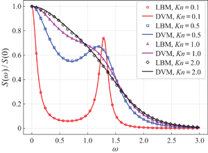
We first investigate the behaviour of the LBM as the number of velocities increases. Shown in figure 5 are the SRBS spectra for a range of  ${\textit {Kn}}$ from 0.1 to 2.0 as computed by the LBM using rules with an increasing number of velocities of both P1 and P2 groups. For reference, the DVM result and the theoretical predictions for the continuum and free-molecular flow limits, (2.23) and (2.17), respectively, are also shown. At
  ${\textit {Kn}}=0.1$, all are in good agreement. As
  ${\textit {Kn}}$ increases beyond 0.5, when the rarefaction effect starts to become significant, as indicated by the deviation between the DVM and NSF solutions, all the way up to
  ${\textit {Kn}}=2.0$, when DVM almost agrees with (2.17), the results of the LBM using higher-order rules, especially those in the P1 group, track those of the DVM quite well, while the LBM results using lower-order rules depart from those of the DVM.

Figure 5. Normalized SRBS spectra predicted by the LBM with quadrature rules of various orders. From top to bottom, the Knudsen number in each row is respectively 0.1, 0.5, 1.0 and 2.0. The LBM results (markers) using the P1 and P2 rules are shown in the left and right columns, respectively. The reference result using the DVM (dashed line), theoretical predictions from the NSF equations (2.23) (solid line) and free-molecular flow (2.17) (dash-dotted line) are also shown for comparison. Here 100 spatial cells are used and the perturbation density intensity is  $\varepsilon = 10^{-5}$ in the LBM.
To reveal the trend of increasing  ${\textit {Kn}}$ for particular rules, shown in figure 6 are the SRBS spectra by the LBM with the two D1Q37 rules for the same range of
  ${\textit {Kn}}$. All can be seen to be in good agreement with the DVM, except that the result using the P2 rule starts to deviate at
  ${\textit {Kn}}=2.0$.

Figure 6. Normalized SRBS spectra calculated by the LBM (empty markers) with D1Q37P1 (a) and D1Q37P2 (b) compared with reference DVM results (solid line).
To quantify the deviation, we define the overall relative error as
 \begin{equation} \mathrm{error} = \frac{\displaystyle \int_{0}^{\infty}|S - S^{DVM}|\, \textrm{d} \omega}{\displaystyle \int_{0}^{\infty}S^{DVM}\, \textrm{d} \omega}, \end{equation}
and show in figure 7 the errors for the same range of  ${\textit {Kn}}$ by the two groups of rules. For the purpose of demonstrating the error sources, results at two spatial resolutions, 100 and 500, are shown. First of all, at
  ${\textit {Kn}} = 2.0$, the error monotonically decreases with the increasing number of velocities independent of spatial resolution for both P1 and P2 rules. This can be explained as that the overall error at this
  ${\textit {Kn}}$ is mainly due to the strong rarefaction effect's not being adequately captured by the LBM system. The discretization error is small and overshadowed. Also to be noted is that the P1 rules consistently outperform the P2 rules, which will be explained later in the section. At lower
  ${\textit {Kn}}$, the decreases of the errors are more rapid as the rarefaction effect is weaker and can be captured by the LBM system with fewer number of velocities. The decreases stop at some points that depend on
  ${\textit {Kn}}$ and then the errors start to increase slowly. At this stage, the errors depend strongly on the spatial resolution, indicating that they are mainly due to spatial discretization.

Figure 7. Relative error of the LBM-predicted SRBS spectra with respect to the DVM results. Shown in the left and right columns are results using cell number  $N=100$ and
  $500$, and in the top and bottom rows are results using the P1 and P2 rules. Note the interplay of the error due to rarefaction, which decreases monotonically with the increasing number of velocities but is independent of the spatial resolution, and that due to spatial discretization, which depends strongly on the spatial resolution but only weakly on the number of velocities.
Shown in figure 8 are the numbers of velocities needed for the relative error between the LBM and DVM to be within 1 % as a function of  ${\textit {Kn}}$. For comparison, the same numbers are also shown for the FVM solution of (3.7) using GH rules as detailed in § 3.2. In order to analyse the performance of discrete velocity quadratures, sufficient spatial cells should be employed to avoid possible contamination. As expected, the P1, P2 and GH rules can reach high accuracy with sufficient number of velocities. Particularly, P1 rules with 19 points can be within 1 % of the DVM for
  ${\textit {Kn}}$ up to 1.7. Also to be noted is that, at high
  ${\textit {Kn}}$, the FVM with GH rules requires significantly more velocities to reach the same accuracy level even though GH rules have degrees of precision twice those of P1 and P2. The phenomenon that GH rules have a relatively poor effect in capturing the rarefaction behaviour was also observed in Wu & Gu (Reference Wu and Gu2020).

Figure 8. The number of minimum discrete velocities to achieve the convergence against  ${\textit {Kn}}$. The red, blue and green lines are, respectively, the results of the LBM with P1 and P2, and the FVM with GH rules. A uniform mesh of 100 cells is used in the LBM, while 640 cells is used in the FVM, with one exception of 2560 cells at
  ${\textit {Kn}}=0.1$ because of strict convergence criteria. The CFL number is set to 0.2 in the FVM.
To give a possible explanation for the different accuracy characteristics among the three classes of quadrature rules, we show in figure 9 the real part of the spatial and temporal Fourier-transformed perturbation distribution function at  ${\textit {Kn}}=2.0$:
 \begin{equation} \hat{\phi}_1(\xi,{\textit{Kn}},\omega)=\int_{0}^{\infty}\int_{-\infty}^{\infty} \textrm{e}^{\textrm{i}(x-\omega t)}[\psi_1 - \psi^{(0)}]\, \textrm{d} x\, \textrm{d} t. \end{equation}
Note that the SRBS spectrum is the integral of the real part of  $\hat {\phi }_1(\xi ,{\textit {Kn}},\omega )$ with respect to
  $\xi$, namely
 \begin{equation} S({\textit{Kn}},\omega)=2\int_{-\infty}^\infty \mathrm{Re}[\hat{\phi}_1(\xi,{\textit{Kn}},\omega)]\, \textrm{d} \xi. \end{equation}
It can be observed that the distribution function is non-negligible roughly in the velocity interval of  $[-5,5]$ in which the number of discrete velocities is different among the three groups of rules. There are more velocities in P1 situated in this interval than in GH and P2. To verify the influence of velocity interval, we note from figure 8 that GH40 can achieve convergence at
  ${\textit {Kn}}=2.0$ with the minimum velocity interval
  $0.4937$, which is close to the lattice constant
  $0.4854$ of D1Q27P1.

Figure 9. The real part of the Fourier-transformed perturbation distribution function  $\hat {\phi }_1(\xi ,{\textit {Kn}},\omega )$ when
  ${\textit {Kn}}=2.0$: (a)
  $\omega =0.0$; (b)
  $\omega =2.0$. Circles, squares, triangles and solid lines are, respectively, the results of the LBM with D1Q27P1, LBM with D1Q27P2, FVM with GH27, and DVM. Note that
  $\hat {\phi }_1$ is normalized by
  $\varepsilon ^2$.
4.2. Comparison of the LBM and FVM
In this subsection, we evaluate the performance of the LBM and FVM in the whole regime in terms of accuracy and computational efficiency. It has been recognized that the traditional FVM, where the time step and cell size are limited by the mean collision time and mean free path of gas molecules, work well for highly rarefied gas flow (Dimarco & Pareschi Reference Dimarco and Pareschi2014).
Shown in table 3 is the relative error of SRBS spectra using the LBM and FVM in comparison with the DVM reference results in the rarefied regime. For fair comparison, the D1Q37P1 rule is implemented in the LBM and FVM. Because of the large mean collision time in the rarefied regime, the time step in the FVM is limited only by the CFL condition. For the unsteady problem, the total physical time is set to 120 such that the density perturbation is sufficiently close to 0 and the SRBS spectra are accurate enough. It can be found that good accuracy can be achieved with the FVM as long as  $\mathrm {CFL}<1.0$. Interestingly, the error of the FVM decreases monotonically with the increase of the CFL number at the same mesh size. In addition, it is observed that the LBM can give more accurate results than the FVM with the same mesh size when
  ${\textit {Kn}}=0.5$,
  $1.0$ and
  $2.0$. To study the computational time, we run the simulations involved on a PC with an Intel Xeon 2.6 GHz CPU. The efficiency comparison of the LBM and FVM is displayed in figure 10. Since the computational time is independent of the Knudsen number, only the case
  ${\textit {Kn}}=0.5$ is presented. It can be seen that, when the grid number is large, the computational times of the FVM and LBM are directly proportional to the square of the grid number, which can be explained as that the time step is inversely proportional to the grid number. What is more, the computational time of the FVM is approximately 10 times that of the LBM with the same cell size, though the CFL number is 0.95 in the FVM. Hence, it can be concluded that the LBM has advantages over the FVM in capturing the rarefaction effects in terms of accuracy and computational efficiency.

Figure 10. Computational time of the FVM and LBM using D1Q37P1 rule at  ${\textit {Kn}}=0.5$. Since the computational time is inversely proportional to the time step, only the cases of CFL number
  $\alpha =0.95$ are present.
Table 3. Relative error of the LBM- and FVM-predicted SRBS spectra with respect to the DVM results for a range of  ${\textit {Kn}}$, i.e. 0.5, 1.0 and 2.0. Here the D1Q37P1 rule is used in both methods for fair comparison; and
  $N$ denotes the cell size.

Shown in figure 11 is the comparison of the accuracy of the LBM and FVM at  ${\textit {Kn}} = 10^{-4}$ in a qualitative way. Unlike the cases in the rarefied regime, the initial density perturbation is set to
  $10^{-6}$ to avoid the nonlinear effect as much as possible and quadruple precision is used in the continuum regime. It can be observed that the results of the LBM show good agreement with the theoretical solution (2.28). Nevertheless, the results of the FVM exhibit a strong dissipation and deviate seriously from the theoretical solutions. A quantitative analysis on the accuracy of the LBM and FVM is performed by extracting the viscosity and thermal diffusivity from numerical simulation results. First,
  $\rho '_k(t)$ is obtained by performing the spatial Fourier transform on the density perturbation field at each time step. Then it is fitted with the theoretical model (2.28) and (2.29a,b) using the Levenberg–Marquardt algorithm to determine the viscosity and thermal diffusivity. Note that the total time is set to 960 in the LBM and FVM so as to extract reliable parameters.

Figure 11. Typical time histories of  $\rho '_k(t)/\rho '_k(0)$ as predicted by the LBM and FVM at
  ${\textit {Kn}}=10^{-4}$. Here the D1Q5P1 rule and cell number
  $N=40$ are used in both the LBM and FVM. The density impulse intensity
  $\varepsilon =10^{-6}$ and quadruple precision are used in the above computation. The CFL number
  $\alpha =0.01$ in the FVM. The blue, green and red lines denote the results of the FVM, LBM and NSF solutions of (2.28), respectively.
A well-known issue with the FVM scheme of (3.13) is its high numerical dissipation in the continuum regime that results in small time step and cell size. Since the convective and collision terms of the Boltzmann model equation are discretized into a completely explicit form shown in (3.13), the time step (3.18) and cell size have to be constrained by the relaxation time and mean free path in order to have acceptable stability and accuracy. If the spatial cell size is not smaller than the mean free path, the numerical transport coefficients, e.g. viscosity and thermal conductivity, might be much larger than the physical ones (Wang et al. Reference Wang, Ho, Wu, Guo and Zhang2018; Su et al. Reference Su, Ho, Zhang and Wu2020a,Reference Su, Zhu, Wang, Zhang and Wub). On the contrary, the collision term in the LBM is integrated by use of the trapezoidal rule shown in (3.19), which is a semi-implicit time discretization; therefore, the restriction that the time step should be smaller than the mean collision time is removed. More importantly, the advection operator is solved exactly with the on-lattice LBM. Thus, it can be predicted that the on-lattice LBM can give better results than the FVM at the same grid resolution.
The relative error is defined as  $\zeta ^* = |\zeta - \zeta _t|/\zeta _t$, where
  $\zeta _t$ is the theoretical transport coefficient, which is summarized in figure 12 as a function of the number of grid resolutions when
  ${\textit {Kn}}=10^{-3}$ and
  $10^{-4}$. Obviously, the relative error is a direct measure of the numerical dissipation. According to the Chapman–Enskog expansion, D1Q5P1 with a seventh-order quadrature is sufficient to recover the linearized NSF equations. As expected, the on-lattice LBM shows a second-order spatial accuracy. The relative errors of viscosity and thermal diffusivity obtained by the FVM, however, are approximately two orders of magnitude more than that by the LBM at
  ${\textit {Kn}}=10^{-3}$ and the differences further increase to three orders of magnitude when
  ${\textit {Kn}}=10^{-4}$. Additionally, the numerical dissipation in the FVM decreases when the CFL number changes from 0.01 to 0.001, which is consistent with the requirement of a small time step to achieve better accuracy.

Figure 12. Grid convergence of the LBM and FVM. Plotted are the relative errors in viscosity and thermal diffusivity using the D1Q5P1 rule on an  $L$ cell ranging from
  $L=20$ to
  $L=320$. The density impulse intensity
  $\varepsilon =10^{-6}$ and quadruple precision are used in the computations. Shown in the left and right columns are the relative errors of viscosity and thermal diffusivity, and in the top and bottom rows are results when
  ${\textit {Kn}} = 10^{-3}$ and
  $10^{-4}$, respectively.
The computational times of the FVM and LBM are shown in figure 13, and the computational time of the FVM with  $\mathrm {CFL} = 0.01$ is more than two orders of magnitude longer than that of the LBM at
  ${\textit {Kn}}=10^{-3}$. Therefore, it can be concluded that the LBM is much superior to the FVM in describing the continuum flow behaviour in terms of accuracy and efficiency. Finally, we perform a comparison of numerical dissipation of the FVM and the FVM without limiter with cell number
  $N=40$ and CFL number
  $\alpha =0.01$ at
  ${\textit {Kn}}=10^{-4}$. Table 4 shows that the FVM without limiter has a lower numerical dissipation, while it is still at least one order of magnitude more than that of the LBM.

Figure 13. Computational time of the FVM and LBM using D1Q5P1 at  ${\textit {Kn}}=10^{-3}$. For simplicity, only the cases of CFL number
  $\alpha =0.01$ are shown.
Table 4. The extracted viscosity and thermal diffusivity obtained by the FVM, the FVM without limiter and the LBM using the D1Q5P1 rule on the cell number 40 when  ${\textit {Kn}}=10^{-4}$. In parentheses are shown the relative errors of viscosity and thermal diffusivity. The CFL number
  $\alpha = 0.01$ is employed in the FVM and the FVM without limiter.

5. Conclusion and discussion
In summary, two kinds of 1-D high-order on-lattice quadratures P1 and P2 have been devised and the accuracy of the on-lattice LBM has been evaluated in the continuum and rarefied regimes by solving the Boltzmann–BGK equation for the spontaneous Rayleigh–Brillouin scattering problem. Our results show that the high-order on-lattice LBM can capture the rarefaction effect accurately and, since more discrete velocities in P1 are distributed in the domain where the distribution function is not negligible, P1 performs better than P2 and GH rules in the rarefied regime. That is, to achieve the same level of accuracy, the on-lattice LBM with P1 quadrature needs less discretized velocity grids than P2 and GH rules. In comparison with the FVM, the on-lattice LBM has a much lower numerical dissipation and can capture the hydrodynamic behaviour accurately and efficiently without requiring small time step and spatial cell size in the continuum regime.
In this work we mainly focus on the case without the gas–wall interaction, which is an important aspect of rarefied gas flow, to evaluate the accuracy of the high-order on-lattice LBM, and the cases with gas–wall interaction will be considered in the future. In addition, we note that half-range quadrature is more advantageous than full-range quadrature to capture the effects of gas–wall interaction (Ambruş & Sofonea Reference Ambruş and Sofonea2016a,Reference Ambruş and Sofoneab); the method of constructing the present on-lattice quadrature can also be applied to design the half-range high-order on-lattice quadrature.
Acknowledgements
This work was supported by the National Science Foundation of China (grant numbers 91741101 and 91752204), Department of Science and Technology of Guangdong Province (grant number 2019B21203001), Shenzhen Science and Technology Program (grant number KQTD20180411143441009) and Science and Technology Innovation Committee of Shenzhen (grant number K19325001).
Declaration of interests
The authors report no conflict of interest.


