3.1 Mean velocity and Reynolds stresses profiles

Profiles of the mean velocity and Reynolds stresses are presented in figure 7. The statistics are calculated from 17 689 velocity fields acquired over a duration of 2.95 s $(2.8\times 10^{4}\unicode[STIX]{x1D70F}_{\unicode[STIX]{x1D708}})$ . The spatially averaged integral time scale $\unicode[STIX]{x1D70F}=\int R_{u,u}\,\text{d}s$ , where $R_{u,u}(s)$ is the autocorrelation function of the streamwise velocity, is 0.0115 s. As a result, data acquisition time corresponds to $257\unicode[STIX]{x1D70F}$ . The spatially averaged mean velocity profile (figure 7 a) is compared with the log-law profile: $U^{+}=(1/\unicode[STIX]{x1D705})\ln y^{+}+B$ , where $\unicode[STIX]{x1D705}=0.41$ and $B=5.2$ , as well as with $U^{+}=y^{+}$ in the viscous sublayer (Pope Reference Pope2000). The wall-normal distance is normalized using $h$ , indicated in the bottom axis, and using $\unicode[STIX]{x1D6FF}_{\unicode[STIX]{x1D708}}$ shown in the top axis. This velocity profile calculated from the ‘standard’ TPIV shows a clear log-law region, but it is erroneous, as expected, in the buffer layer, where a vector spacing of $l^{+}=20.6$ is too coarse. Two related techniques are utilized to extract the near-wall velocity. The first one is the sum-of-correlation method (Meinhart, Wereley & Santiago Reference Meinhart, Wereley and Santiago2000), which determines the mean velocity at each location from an ensemble-averaged correlation map for small interrogation windows. To enhance the particle image concentrations, in the present calculation, the 3D particle distributions are projected onto 2D images by assigning the maximum intensity along the spanwise direction to each pixel. The ensemble-averaged distribution of correlations is calculated for an $8\times 8$  pixels interrogation window with 75 % overlap. An alternative approach is the ‘single-pixel ensemble correlation’ (Westerweel, Geelhoed & Lindken Reference Westerweel, Geelhoed and Lindken2004; Scharnowski, Hain & Kahler Reference Scharnowski, Hain and Kahler2012; Soria & Willert Reference Soria and Willert2012), which is equivalent to reducing the interrogation window down to one pixel. These calculations are also performed using the above-mentioned 2D projected images. Results of both techniques are also included in figure 7(a). Evidently, they extend the velocity profile down to the buffer layer, but deviate from the expected linear velocity profile for $y^{+}<\sim 2$ . This deviation is not surprising considering that the particle diameter is approximately $1.2\unicode[STIX]{x1D6FF}_{\unicode[STIX]{x1D708}}$ .

The Reynolds stresses profiles, $\langle u^{\prime }u^{\prime }\rangle /u_{\unicode[STIX]{x1D70F}}^{2}$ , $\langle v^{\prime }v^{\prime }\rangle /u_{\unicode[STIX]{x1D70F}}^{2}$ , $\langle w^{\prime }w^{\prime }\rangle /u_{\unicode[STIX]{x1D70F}}^{2}$ , $-\langle u^{\prime }v^{\prime }\rangle /u_{\unicode[STIX]{x1D70F}}^{2}$ , and $p_{rms}/\unicode[STIX]{x1D70C}u_{\unicode[STIX]{x1D70F}}^{2}$ are presented in figure 7(b). The distribution of $\langle u^{\prime }u^{\prime }\rangle /u_{\unicode[STIX]{x1D70F}}^{2}$ peaks near the wall, considering that the buffer layer is not resolved, followed by a plateau extending to $y/h\sim 0.1(y^{+}\sim 230)$ . Both have been observed before in experiments and simulations (e.g. Hutchins & Marusic Reference Hutchins and Marusic2007a ; Mathis, Hutchins & Marusic Reference Mathis, Hutchins and Marusic2009; Hultmark, Bailey & Smits Reference Hultmark, Bailey and Smits2010; Marusic, Mathis & Hutchins Reference Marusic, Mathis and Hutchins2010; Mathis, Hutchins & Marusic Reference Mathis, Hutchins and Marusic2011; Hultmark Reference Hultmark2012; Schultz & Flack Reference Schultz and Flack2013; Bernardini, Pirozzoli & Orlandi Reference Bernardini, Pirozzoli and Orlandi2014; Lee & Moser Reference Lee and Moser2015). The height of the plateau is also consistent with those of Schultz & Flack (Reference Schultz and Flack2013) for similar $Re_{\unicode[STIX]{x1D70F}}$ . By inspecting the energy spectra of the streamwise velocity at various elevations, Hutchins & Marusic (Reference Hutchins and Marusic2007a ) associate the plateau with energy contributed by large-scale log-layer motions. They also demonstrate that these large-scale structures modulate the amplitude of the near-wall streamwise velocity fluctuations, a phenomenon relevant to the present investigation. The Reynolds shear stress $-\langle u^{\prime }v^{\prime }\rangle /u_{\unicode[STIX]{x1D70F}}$ peaks around $y/h\sim 0.12(y^{+}\sim 280)$ . As shown in Zhang et al. (Reference Zhang, Miorini and Katz2015), we estimate the wall stress by extrapolating the total shear stress, namely the sum of the viscous and Reynolds stresses, to the wall. The result is used for normalizing all the present ensemble-averaged variables, and agrees with the mean velocity profile (figure 7 a). The elevation of the Reynolds stress peak is slightly higher than those found in Hoyas & Jiménez (Reference Hoyas and Jiménez2006) and Schultz & Flack (Reference Schultz and Flack2013) at similar Reynolds numbers ( $Re_{\unicode[STIX]{x1D70F}}=2000$ ). It is presumably associated with the size of the TPIV interrogation volume of $82.3\unicode[STIX]{x1D6FF}_{\unicode[STIX]{x1D708}}$ , which attenuates the small-scale fluctuations near the wall (Hong et al. Reference Hong, Katz and Schultz2011; Talapatra & Katz Reference Talapatra and Katz2013). The values of $p_{rms}/\unicode[STIX]{x1D70C}u_{\unicode[STIX]{x1D70F}}^{2}$ decrease with elevation, consistent with those reported in Tsuji et al. (Reference Tsuji, Fransson, Alfredsson and Johansson2007) and Joshi et al. (Reference Joshi, Liu and Katz2014) for boundary layers at similar Reynolds numbers. DNS results for channel flow at $Re_{\unicode[STIX]{x1D70F}}=1020$ by Abe, Matsuo & Kawamura (Reference Abe, Matsuo and Kawamura2005) show a similar trend with elevation, but their magnitudes are lower by approximately 50 %. An increase in pressure fluctuations with increasing Reynolds number has been observed experimentally (Tsuji et al. Reference Tsuji, Fransson, Alfredsson and Johansson2007) and in simulated data (Lozano-Durán & Jiménez Reference Lozano-durán and Jiménez2014).

3.2 Spectra of pressure and deformation

The spatial power spectral density (PSD) of pressure, $E_{pp}(k_{x})$ , normalized by $\unicode[STIX]{x1D70F}_{w}^{2}\unicode[STIX]{x1D708}/u_{\unicode[STIX]{x1D70F}}$ , at two elevations are presented in figure 8. Here, $k_{x}=2\unicode[STIX]{x03C0}/\unicode[STIX]{x1D706}_{x}$ is the streamwise wavenumber. For the current analysis, we opt to present directly measured spatial spectra because, as noted before, by setting the spatially averaged instantaneous pressure to zero, the pressure signal is spatially high-pass filtered. Hence, it is also expected to attenuate a not readily determined part of the frequency spectrum. The spectra are calculated using FFT without windowing using all the instantaneous realizations over the entire spanwise range, and then spatially and ensemble-averaged. The results are normalized with inner scaling and compared with the measured PSD of pressure calculated from planar PIV data (Joshi et al. Reference Joshi, Liu and Katz2014) in the same facility, but for a developing boundary layer. The axes normalized with outer scaling are added for comparison, based on the present experimental conditions. The present results are also compared to the PSD of DNS-based wall pressure data of Abe et al. (Reference Abe, Matsuo and Kawamura2005) for channel flow. At low wavenumbers, the present results agree with those of Joshi et al. (Reference Joshi, Liu and Katz2014) for the same elevation. However, they deviate at high wavenumbers, with the present values being lower, presumably owing to differences in the dimensionless spatial resolution. In Joshi et al. (Reference Joshi, Liu and Katz2014), the interrogation window size is $35.8\unicode[STIX]{x1D6FF}_{\unicode[STIX]{x1D708}}$ versus $82.3\unicode[STIX]{x1D6FF}_{\unicode[STIX]{x1D708}}$ for the present data. Furthermore, the 75 % overlap utilized in the TPIV analysis also causes aliasing at high wavenumbers (Foucaut, Carlier & Stanislas Reference Foucaut, Carlier and Stanislas2004; Schrijer & Scarano Reference Schrijer and Scarano2008). The present PSD is higher than that of Abe et al. (Reference Abe, Matsuo and Kawamura2005), presumably due to differences in Reynolds number, consistent with trends shown by them.

Figure 8. The present power spectral density of pressure compared with previous experimental and DNS results.

The PSD of the deformation, $E_{dd}(\unicode[STIX]{x1D714})$ , normalized by $h(\unicode[STIX]{x1D70C}u_{\unicode[STIX]{x1D70F}}^{2}l_{0}/E^{\prime })^{2}/U_{0}$ , calculated from the small FOV data is shown in figure 9(a). The spectrum is calculated for each surface node for the entire duration of the measurement, and then spatially averaged. As is evident, the surface motions involve a broad range of time scales, with an r.m.s. value of $42~\unicode[STIX]{x03BC}\text{m}$ . Part of the motions are associated with channel vibrations, whose length scales are presumably much larger than the FOV. Hence, they displace or tilt the entire FOV. Bi-directional linear detrending of instantaneous realization filters these motions out, as done for the rest of this paper. The PSD of the detrended deformation is shown in figure 9(b). The corresponding r.m.s. value is $0.2~\unicode[STIX]{x03BC}\text{m}$ ( $0.02\unicode[STIX]{x1D6FF}_{\unicode[STIX]{x1D708}}$ ). Hence, the present detrended deformations are not expected to have a significant impact on the flow structure in the boundary layer, resulting in a ‘one-way coupling’, where the flow affects the wall, but not vice versa. After detrending, the spectrum has two troughs, at $\unicode[STIX]{x1D714}h/U_{0}\sim 1.6$ and ${\sim}4.3$ . i.e. it can be roughly divided into three frequency bands: (i)  $f<25~\text{Hz}$ or $\unicode[STIX]{x1D714}h/U_{0}<1.6$ , (ii)  $25~\text{Hz}<f<67~\text{Hz}$ and (iii)  $f>67$  Hz or $\unicode[STIX]{x1D714}h/U_{0}>4.3$ , as indicated by two vertical lines. A visual inspection of the temporally filtered deformation for each of these bands (see supplementary movies 2–4) indicates that only deformations in the highest frequency band are dominated by downstream-travelling surface patterns. The dominant motions in the first and second bands seem to propagate in all directions, and sometimes behave like standing waves. It should be noted that these waves have much lower amplitude and they occur at much lower velocity (relative to the  $c_{t}$ ) than the static-divergence wave reported in Hansen & Hunston (Reference Hansen and Hunston1974, Reference Hansen and Hunston1983) and Gad-el-Hak et al. (Reference Gad-el-Hak, Blackwelder and Riley1984). The PSD of the detrended deformation for the large FOV is presented in figure 10. The corresponding r.m.s. value is $0.18~\unicode[STIX]{x03BC}\text{m}$ , still much smaller than the wall unit, and are not expected to have a significant effect on the flow structure. The location of trough at $\unicode[STIX]{x1D714}h/U_{0}\approx 1.6$ –1.8 is consistent with that shown in figure 9(b), but $\unicode[STIX]{x1D714}h/U_{0}=1.8$ also corresponds to a deformation with wavelength equal to the length of the sample area (90 mm) travelling at a velocity of 2.5 m s $^{-1}$ , the centreline velocity. The peaks at $\unicode[STIX]{x1D714}h/U_{0}<1.8$ correspond to non-advected phenomena, and do not have a consistent direction of propagation. In subsequent analysis, most of our attention focuses on the advected phenomena. The large FOV spectrum does not have a trough at $\unicode[STIX]{x1D714}h/U_{0}\sim 4.3$ , confirming that the dip in figure 9(b) is caused by detrending.

Figure 9. Power spectral density of the normalized deformation (a) before spatial detrending and (b) after spatial detrending. Reprinted with permission from Springer.

Figure 10. Power spectral density of the large field-of-view detrended deformation. The lines show predictions of the Chase (Reference Chase1991) model for flat pressure spectra with phase speeds of $0.72U_{0}$ (dash-dot line) and $U_{0}$ (dashed line), as well as the measured pressure spectra at $y/h=0.03$ for a phase speed of $0.72U_{0}$ (thick line).

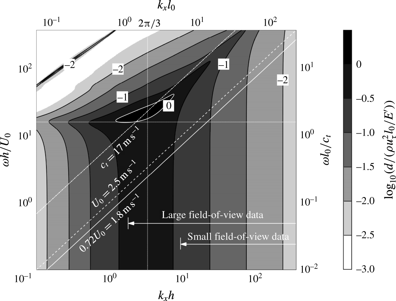
Figure 11. The amplitude of deformation (normalized by $\unicode[STIX]{x1D70C}u_{\unicode[STIX]{x1D70F}}^{2}l_{0}/E^{\prime }$ ) in response to pressure perturbation amplitude of $\unicode[STIX]{x1D70C}u_{\unicode[STIX]{x1D70F}}^{2}$ , as predicted by the Chase (Reference Chase1991) model. The inclined lines correspond to the specified advection speeds. The vertical and horizontal dotted lines represent $k_{x}l_{0}=2\unicode[STIX]{x03C0}/3$ and $\unicode[STIX]{x1D714}l_{0}/c_{t}=1.45$ , respectively.

To elucidate the shape of the spectrum for $\unicode[STIX]{x1D714}h/U_{0}>1.8$ , one can analyse the response of a compliant layer to pressure perturbations. Chase (Reference Chase1991) introduces a classical model for the response of a viscoelastic layer under prescribed pressure and wall shear stress fluctuations. Because of its significance to the present study, the model is summarized in appendix A. Briefly, this 2D model involves streamwise and wall-normal small-amplitude deformations in a domain with thickness of $l_{0}$ unbounded in the $x$ -direction. Using Helmholtz decomposition, the displacement and stresses of the compliant layer are solved for a viscoelastic material. The material damping is accounted for by allowing complex longitudinal and shear wave speeds in the Navier equation. The prescribed pressure, shear as well as fluid loading serve as boundary conditions. As shown in appendix  A, for the present range of frequencies, wavenumbers, material properties, and magnitude of pressure fluctuations relative to those of shear stresses (Tsuji et al. Reference Tsuji, Fransson, Alfredsson and Johansson2007, Reference Tsuji, Imayama, Schlatter, Alfredsson, Johansson, Marusic, Hutchins and Monty2012), the impact of pressure on the shape of the wall is higher by orders of magnitudes than that of shear stresses. Hence, the present analysis focuses on the effect of pressure. Figure 11 shows the normalized wavenumber–frequency spectrum of wall deformation predicted by the Chase (Reference Chase1991) model for sinusoidal pressure excitation with equal amplitude ( $=\unicode[STIX]{x1D70C}u_{\unicode[STIX]{x1D70F}}^{2}$ ) at all wavenumbers and frequencies. Both the frequency and wavenumber are normalized using two different variables, with those involving $l_{0}$ and $c_{t}$ being associated with the model directly, and those involving $h$ and $U_{0}$ being added in order to relate the results to the flow conditions. The peak response occurs at $k_{x}l_{0}\approx 2\unicode[STIX]{x03C0}/3$ . At higher wavenumbers, i.e. to the right of the vertical dotted line, the surface response peaks when the pressure phase speed is slightly lower than $c_{t}$ . The latter is highlighted by the inclined dash-dot line. Evidently, since the present centreline velocity, which is indicated by a dash line, is much lower than $c_{t}$ , the interactions between the compliant wall and the flow are substantially weaker than the peak values.

For $\unicode[STIX]{x1D714}l_{0}/c_{t}<1.45$ , the surface response over the entire domain has a broad peak centred at $k_{x}l_{0}\approx 2\unicode[STIX]{x03C0}/3$ . For the current study, the peak wavelength, $3l_{0}$ , is equal to $1.89h$ . Hence, this wavelength is covered by the large FOV, but not by the small FOV, as highlighted in figure 11. Consequently, the deformation features dominating the large FOV data (figure 6) have a wavelength of ${\sim}1.9h$ , which cannot be observed in the small FOV. The vertically aligned spectral peak at low frequencies ( $\unicode[STIX]{x1D714}l_{0}/c_{t}<1.45$ ) indicates that the wavenumber corresponding to the spectral peak is only a function of $l_{0}$ , and does not depend on the phase speed of the pressure perturbation. Consequently, within this spectral domain, one can readily tailor the surface response to flow excitation by varying the compliant layer thickness. This statement is relevant to cases involving stiff compliant material, where the shear speed is significantly higher than the flow speed. At low wavenumbers ( $k_{x}l_{0}<2\unicode[STIX]{x03C0}/3$ ), the surface response is high at a frequency of $\unicode[STIX]{x1D714}l_{0}/c_{t}\approx 1.45$ , i.e. slightly below $\unicode[STIX]{x03C0}/2$ , as indicated by a horizontal dotted line. This frequency corresponds to two roundtrips across the compliant layer at a phase speed of $c_{t}$ . For the present experimental conditions, advected phenomena in the relevant frequency range have a very short wavelength. Hence, the present conditions do not fall in the relevant frequency–wavenumber bandwidth to excite these modes.

For flow features propagating at the centreline velocity or similar values ( $U_{0}$ and $0.72U_{0}$ are shown in figure 11), the intersection of the phase speed with the wavenumber–frequency spectrum provides a prediction for the frequency spectrum. This prediction assumes that the amplitude of pressure perturbations does not vary with frequency. The resulting spectra are presented as the flat $E_{pp}$ lines in figure 10 for pressure excitation with advection speeds of $0.72U_{0}$ and $U_{0}$ , and amplitude of 1.3 $\unicode[STIX]{x1D70C}u_{\unicode[STIX]{x1D70F}}^{2}$ . This amplitude is selected to match that of the measured $E_{dd}$ . As is evident, the shapes of the predicted and measured deformation spectra appear to agree for frequencies falling in the $1<\unicode[STIX]{x1D714}h/U_{0}<12$ range. The frequency of the peak response at $\unicode[STIX]{x1D714}h/U_{0}\approx 4$ , is better predicted when $U_{0}$ is used as the advection speed. The analysis can be repeated for frequency- (or wavenumber-)dependent pressure amplitude using the measured pressure spectrum (figure 8). The result, which is also presented in figure 10 and labelled as ‘measured $E_{pp}$ ’ is based on the pressure spectrum, including amplitude, at $y/h=0.03$ ( $y^{+}=70$ ). This spectrum has a similar shape as the others, but values are lower, and the peak location agrees with that corresponding to an advection speed of $0.72U_{0}$ . It appears that the Chase (Reference Chase1991) model predicts the response of the present ‘stiff’ compliant wall to advected pressure excitation. Conversely, below $\unicode[STIX]{x1D714}h/U_{0}\approx 1$ , the model and measured spectra diverge, presumably, since this range is dominated by features that are not advected with the flow, as the deformation movies show (supplementary movie 2). They might be associated with, for example, resonances or reflected waves associated with the finite boundaries of the compliant wall.

The measured streamwise wavenumber–frequency spectra of detrended deformation, $E_{dd}(k_{x},\unicode[STIX]{x1D714})$ , normalized by $[h(\unicode[STIX]{x1D70C}u_{\unicode[STIX]{x1D70F}}^{2}l_{0}/E^{\prime })]^{2}/U_{0}$ for the small and large FOV are presented in figure 12(a,b), respectively. They are calculated separately for each spanwise location using FFT in the streamwise and time directions. The resulting spectra are then spanwise-averaged. The small FOV data, which is presented on linear scales, has two inclined bands representing two advection modes of different speeds, which are presumably associated with flow structures located at different elevations in the boundary layer. In subsequent discussions, we refer to them as a ‘slow mode’, with an advection speed of $0.72U_{0}$ , and a ‘fast mode’ with speed of $U_{0}$ . The choices of pressure advection speeds in figure 11 are based on these modes. The fast mode band extends to higher frequencies and wavenumbers than the slow mode. The simulation of Kim & Choi (Reference Kim and Choi2014) also show a preferred advection speed of $0.72U_{0}$ , for stiff compliant surfaces, consistent with the present slow mode, but do not show a fast mode. At low frequencies, i.e., $\unicode[STIX]{x1D714}h/U_{0}<4.3$ , the spectral contours are largely aligned in the horizontal direction, indicating that this range is dominated by non-advected features with nearly zero phase speed. Such bands have also been observed in the DNS results of Kim & Choi (Reference Kim and Choi2014), which they attribute to resonances of the spring and damper system that they utilize to model the compliant wall.

Figure 12. The measured wavenumber–frequency spectra of detrended deformation, with contours indicating the values of $\log _{10}\{E_{dd}(k_{x},\unicode[STIX]{x1D714})U_{0}/[h(\unicode[STIX]{x1D70C}u_{\unicode[STIX]{x1D70F}}^{2}l_{0}/E^{\prime })]^{2}\}$ . (a) Small field-of-view data on linear axes, with an incremental increase between contour lines of 0.15. (b) Large field-of-view data on logarithmic axes, with an incremental increase between contour lines of 0.3. The inclined solid and dashed lines represent advection speeds of $0.72U_{0}$ and $U_{0}$ , respectively. The vertical lines in each figure show the wavenumber of the corresponding field of view.

Figure 13. (a–c) Wavenumber–frequency spectra of pressure at (a) $y/h=0.35$ , (b)  $y/h=0.12$ and (c) $y/h=0.05$ . (d–f) Pressure–deformation wavenumber–frequency cross-spectra at (d) $y/h=0.35$ , (e) $y/h=0.12$ and (f) $y/h=0.05$ . The dashed lines, solid lines and dotted lines correspond to phase speeds of $U_{0}$ , $0.72U_{0}$ and the local mean velocity, respectively. The vertical lines in each figure show the wavenumber of the corresponding field of view. The grey scales on (a–c) and (d–f) indicate the values of $\log _{10}\{E_{pp}(k_{x},\unicode[STIX]{x1D714})U_{0}/[h(\unicode[STIX]{x1D70C}u_{\unicode[STIX]{x1D70F}}^{2})]^{2}\}$ and $\log _{10}\{E_{pd}(k_{x},\unicode[STIX]{x1D714})U_{0}/[h^{2}(\unicode[STIX]{x1D70C}u_{\unicode[STIX]{x1D70F}}^{2})(\unicode[STIX]{x1D70C}u_{\unicode[STIX]{x1D70F}}^{2}l_{0}/E^{\prime })]\}$ , respectively.

The $k_{x}$ - $\unicode[STIX]{x1D714}$ spectrum for the large FOV (figure 12 b) is presented in logarithmic scale to highlight the low-frequency/wavenumber range. Here, at low wavenumber/frequency, the advection band is dominated by the fast mode, which is marked by a white dashed line. At high frequencies, the peak appears to tilt towards lower phase speeds, which falls between the fast and slow modes, the latter being marked by a solid white line. The differences between figure 12(a,b) for overlapping wavenumber ranges, in particular the lack of a distinct slow mode in the latter, can be attributed to the scale of the low-pass filtering and detrending. For a given frequency, large scales are attenuated more than small ones with decreasing filter size. Consequently, the fast mode is attenuated more than the slow mode in the detrended small FOV data, making the latter more visible. This effect has been verified by detrending the large FOV data at the small FOV scales. Results (not shown) confirm that the slow mode becomes more noticeable. Figure 12(b) also shows that energy corresponding to the fast mode extends to scales that are larger than the small FOV ( $k_{x}h<9.4$ ), consistent with the visual observations of large-scale deformation features moving at the centreline velocity (e.g. figure 6). With increasing FOV, the measurements should cover advected features that have frequencies falling below $\unicode[STIX]{x1D714}h/U_{0}\sim 4.3$ . Indeed, figure 12(b) shows that part of the energy at $\unicode[STIX]{x1D714}h/U_{0}<4.3$ corresponds to advected modes at low wavenumbers, where the spectral peak is located, but a substantial fraction is not. These features cannot be seen in the detrended small FOV surface shape, leaving only non-advected features at frequencies falling below $\unicode[STIX]{x1D714}h/U_{0}\sim 4.3$ (67 Hz), and creating the spectral dip at this frequency in figure 9(b).

In subsequent discussions, we correlate the flow structure and pressure field to the surface deformation. Considering that for the small FOV experiment, which provides the relevant data, frequencies corresponding to $\unicode[STIX]{x1D714}h/U_{0}<4.3$ do not contain advected modes. In the analysis that follows, the pressure and deformation are high-pass filtered at $\unicode[STIX]{x1D714}h/U_{0}=4.3$ . Intuitively, correlating the flow with the surface shape has to start with the pressure field. Hence, the pressure $k_{x}-\unicode[STIX]{x1D714}$ spectra, $E_{pp}(k_{x},\unicode[STIX]{x1D714})$ at three elevations, namely $y/h=0.35$ , 0.12 and 0.05, are presented in figure 13(a–c), respectively. They are calculated separately for each spanwise location, and then spatially averaged. The corresponding pressure–deformation cross $k_{x}-\unicode[STIX]{x1D714}$ spectra, $E_{pd}(k_{x},\unicode[STIX]{x1D714})$ , aimed at identifying pressure modes that affect the deformation, are presented in figure 13(d–f). They show the amplitude of the Fourier transform of the cross-correlation between deformation and pressure at the specified elevation. Each plot shows the centreline velocity (or the fast mode) as a dashed line, the slow mode, $0.72U_{0}$ , as a solid line, and the local mean velocity as a dotted line. All the pressure spectra show elevated energy at low wavenumber over a broad frequency range. This artefact is a direct result of setting the spatially averaged pressure over the entire sample volume to zero in the present analysis. In reality, this unavailable reference pressure varies in time, and zeroing it introduces a low wavenumber jitter. To partially resolve this problem, Ghaemi & Scarano (Reference Ghaemi and Scarano2013) use the Bernoulli equation to obtain a boundary condition away from the wall. Using this approach to estimate the reference pressure (e.g. on the upper surface) or frequency low-pass filtering of the signal decreases the magnitude of this band (not shown). This band has no significant effect on the present analysis, and we opt not to manipulate the signals further. At all elevations, the pressure spectra contain clear advection bands at speeds that decrease with elevation, and do not differ substantially from the corresponding mean velocity. This advection band is not as distinct at the lowest elevation (figure 13 c), but is still evident. The pressure–deformation cross-spectra in figures 13(d–f) also show clear advection bands at all elevations, with a phase speed that decreases with elevation. For the pressure at $y/h=0.12$ and 0.05, the phase speeds do not differ significantly from the slow mode or the local mean velocity. As for the pressure at $y/h=0.35$ , the advection band is largely concentrated in the low-frequency/wavenumber range, and the advection speed appears to span between the slow mode and the local mean velocity. With increasing frequency, the band tilts more towards the local mean velocity. A comparison between figures 13(a) and 13(d) suggests that the compliant wall is preferentially affected by the large-scale pressure features. With decreasing distance from the wall, the range of scales affecting the wall deformation expands. Assuming that the strength of eddies increases with their size, but their influences decrease with distance from their centre (the latter being clearly true for vortices), the expanding influence band with decreasing distance from the wall should be expected. These findings are consistent with findings of previous wall pressure fluctuations claiming that the observed scale dependence of the advection speeds is associated with the location of eddies in the boundary layer, with the smaller ones being preferentially located closer to the wall (e.g. Willmarth & Wooldridge Reference Willmarth and Wooldridge1962; Bull Reference Bull1967; Blake Reference Blake1970; Wills Reference Wills1970; Dinkelacker et al. Reference Dinkelacker, Hessel, Meier and Schewe1977; Choi & Moin Reference Choi and Moin1990; Jeon et al. Reference Jeon, Choi, Yoo and Moin1999; Ghaemi & Scarano Reference Ghaemi and Scarano2013; Salze et al. Reference Salze, Bailly, Marsden and Juve2015).

3.3 Conditional correlations between deformation and flow variables

This section examines the relations between deformation and flow structure based on spatial correlations between the surface shape and flow variables (pressure, velocity, vorticity, etc.), as well as between pressure and other flow variables. The spatial conditional correlation between two functions, $f(x,y,z,t)$ and $g(x,y,z,t)$ , is defined as

the parameters involved are specified in the subscript, $\unicode[STIX]{x1D70E}_{f}$ and $\unicode[STIX]{x1D70E}_{g}$ are the r.m.s. values of $f$ and $g$ . In all cases, the correlations are calculated based on fluctuating components of each variable, but there is no need to subtract mean values for pressure and deformation because both are high-pass filtered. To highlight phenomena, in many of the correlations, we impose a condition of, for example, a deformation larger or smaller than its r.m.s. value, i.e. $d(x_{0},y_{0},z_{0})>\unicode[STIX]{x1D70E}_{d}$ or $d(x_{0},y_{0},z_{0})<-\unicode[STIX]{x1D70E}_{d}$ , respectively. The condition is indicated in the definition of the variable. In such cases, the r.m.s. values of $f$ and $g$ are still calculated from the original un-conditioned data. In correlations that do not involve any conditions, $R_{f,g}$ is used instead.

Figure 14. Conditional correlations between the detrended and high-pass filtered (at $\unicode[STIX]{x1D714}h/U_{0}=4.3$ ) deformation at $(0,0)$ and pressure, based on (a,b) strong positive deformation ( $d>\unicode[STIX]{x1D70E}_{d}$ ) and (c,d) strong negative deformation ( $d<-\unicode[STIX]{x1D70E}_{d}$ ). The $y$ – $z$ planes in (b,d) correspond to $\unicode[STIX]{x0394}x/h=0.1$ , which is marked by dashed lines in (a,c). The position of peak value is indicated by a  $+$ .

Figure 15. The loss tangent of PDMS based on the current measurement and several other sources.

Distributions of deformation–pressure conditional correlations based on large positive ( $d>\unicode[STIX]{x1D70E}_{d}$ ) event, $R_{d,p}|_{d_{{>}}\unicode[STIX]{x1D70E}d}$ , for the ( $\unicode[STIX]{x0394}x,\unicode[STIX]{x0394}y,\unicode[STIX]{x0394}z=0$ ) and ( $\unicode[STIX]{x0394}x=0.1h,\unicode[STIX]{x0394}y,\unicode[STIX]{x0394}z$ ) planes are presented in figure 14(a,b), respectively. Results conditioned on $d<-\unicode[STIX]{x1D70E}_{d}$ events, $R_{d,p}|_{d<-\unicode[STIX]{x1D70E}d}$ , are shown in figure 14(c,d), respectively. In all cases, the correlations are calculated for all surface points and then spatially averaged. As is evident, for positive deformation (bump), the negative correlation peak is located at $\unicode[STIX]{x0394}x/h\approx 0.1$ and $\unicode[STIX]{x0394}y/h\approx 0.12$ , i.e. the deformation lags behind the negative pressure influencing it most by ${\sim}0.1h$ in the streamwise direction. A second positive correlation peak with lower magnitude is located upstream, representing a high-pressure region. The streamwise separation between the positive and negative correlation peaks is approximately $0.25h$ , suggesting that the length scale of the pressure field relevant to the deformation is approximately $0.5h$ . The mean velocity at $\unicode[STIX]{x0394}y/h=0.12$ , $0.77U_{0}$ , is close to that of the deformation phase speed of the slow mode, $0.72U_{0}$ . It appears that structures affecting the wall deformation are located in the log-layer, at nearly the same elevation of the Reynolds shear stress peak (figure 7 b), and slightly above the plateau in streamwise velocity fluctuations. The resolution of present velocity and pressure measurements is too coarse for probing the buffer layer. However, the resolution of deformation measurements is sufficient for identifying structures as small as $0.015h$ . Yet, the wavenumber–frequency spectra of deformations (figure 12 a) indicate that they are dominated by phenomena having characteristic length scale larger than $0.13h(290\unicode[STIX]{x1D6FF}_{\unicode[STIX]{x1D708}})$ . Eddies with such scales are likely to reside in the log and/or outer layer, and are less likely to be located in the buffer layer. The $y{-}z$ distribution of correlation in figure 14(b) is presented in a plane ( $\unicode[STIX]{x0394}x=0.1h$ ) that coincides with the streamwise peak in figure 14(a). The $y{-}z$ correlation peak is located at the same elevation as that in the perpendicular plane and centred around $\unicode[STIX]{x0394}z=$ 0. The distributions corresponding to negative deformation (figure 14 c,d) appear to be quite similar to those associated with positive deformation, with the same streamwise offsets. However, since $d<-\unicode[STIX]{x1D70E}_{d}$ , a negative correlation indicates positive pressure. Furthermore, the elevation of the correlation peak is slightly higher, which is located at $\unicode[STIX]{x0394}y/h\approx 0.14$ .

The next discussion is aimed at explaining the streamwise offset between pressure and deformation. It involves both the effect of damping by the compliant wall, as well as the structure of the pressure field in the boundary layer. Starting with the damping effect, one can use the Chase (Reference Chase1991) model to estimate phase lag. It requires knowledge of the viscoelastic properties of the compliant material, which are characterized by using complex moduli, i.e., $E^{\prime }+\text{i}E^{\prime \prime }$ , (e.g. Fung Reference Fung1965; Ferry Reference Ferry1970), with $E^{\prime }$ being the storage modulus, and $E^{\prime \prime }$ the loss modulus. The key parameter is the frequency-dependent loss tangent, $\unicode[STIX]{x1D701}=E^{\prime \prime }/E^{\prime }$ . As shown in figure 15, the loss tangent of the PDMS utilized in the present study has only been measured in a low-frequency range (0.1–12 Hz), using the only instrument available to us. Data from several other sources (Fitzgerald & Fitzgerald Reference Fitzgerald, Fitzgerald and Meng1998; Conte & Jardret Reference Conte and Jardret2002; Kulik et al. Reference Kulik, Semenov, Boiko, Seoudi, Chun and Lee2009; Du et al. Reference Du, Cheng, Lu and Zhang2013; Rubino & Loppolo Reference Rubino and Loppolo2016) are compiled in the same plot in order to extend the frequency to conditions that are relevant for the present study. The shaded area in figure 15 covers the range of results of a series of measurements performed by Kulik et al. (Reference Kulik, Semenov, Boiko, Seoudi, Chun and Lee2009) for samples of various sizes. It appears that various results collapse below 10 Hz, but are scattered over a broad range above 67 Hz. To estimate the damping-induced phase lag, we start with $\unicode[STIX]{x1D701}=0.3$ , but repeat the calculation for other values as well. The streamwise offset between wall pressure and surface deformation based on the Chase (Reference Chase1991) model, $\unicode[STIX]{x0394}x_{\unicode[STIX]{x1D701}}$ , is shown in figure 16. Figure 16(a) demonstrates the effect of $\unicode[STIX]{x1D701}$ for pressure waves with wavelengths of $\unicode[STIX]{x1D706}/h=0.5$ , 1.0 and $2.0h$ and advection speeds of $0.72U_{0}$ (lines) and $U_{0}$ (symbols). As is evident, the values $\unicode[STIX]{x0394}x_{\unicode[STIX]{x1D701}}/\unicode[STIX]{x1D706}$ nearly collapse for the relevant range of phase speeds, i.e. $\unicode[STIX]{x0394}x_{\unicode[STIX]{x1D701}}/\unicode[STIX]{x1D706}$ is only weakly dependent on the frequency. The magnitude of $\unicode[STIX]{x0394}x_{\unicode[STIX]{x1D701}}/\unicode[STIX]{x1D706}$ increases with increasing $\unicode[STIX]{x1D701}$ , an expected trend because the associated increase in relaxation time (Ferry Reference Ferry1970). The weak effect of frequency is demonstrated in figure 16(b), which shows the distribution of $\unicode[STIX]{x0394}x_{\unicode[STIX]{x1D701}}/h$ for a fixed loss tangent of 0.3. Clearly, the contour lines are nearly vertical for the relevant range, indicating that varying the phase speed while keeping the wavelength constant has little effect on $\unicode[STIX]{x0394}x_{\unicode[STIX]{x1D701}}$ . Based on figure 14, choosing $\unicode[STIX]{x1D706}=0.5h$ , the model predicts a spatial offset of $0.024h$ , roughly 24 % of the observed value. Using higher (but reasonable) values for $\unicode[STIX]{x1D701}$ , for example, $\unicode[STIX]{x1D701}=0.4$ , would increase $\unicode[STIX]{x0394}x_{\unicode[STIX]{x1D701}}$ to 0.03 $h$ , i.e. it still explains only a fraction of the measured offset. The rest must be related to the structure of the pressure field in the boundary layer.

Figure 16. The streamwise offset between deformation and pressure correlation peak predicted by the Chase (Reference Chase1991) model: (a) values of $\unicode[STIX]{x0394}x_{\unicode[STIX]{x1D701}}/\unicode[STIX]{x1D706}$ for pressure perturbations with the specified wavelengths and advection speeds, and (b) values of $\unicode[STIX]{x0394}x_{\unicode[STIX]{x1D701}}/h$ as functions of wavenumber and frequency for $\unicode[STIX]{x1D701}=0.3$ .

The structure of the pressure field in the channel flow can be inferred from two-point correlation of pressure, $R_{p,p}$ , which is plotted in figure 17 for a reference point located at $y_{0}/h=0.12$ . Consistent with many previous results (e.g. Kim Reference Kim1989; Tsuji et al. Reference Tsuji, Fransson, Alfredsson and Johansson2007; Ghaemi & Scarano Reference Ghaemi and Scarano2013; Joshi et al. Reference Joshi, Liu and Katz2014), the correlation contours are inclined at a rather large angle relative to the mean flow. Using the locus of points along which the correlation value has the slowest decay (white line), the estimated inclination angle around $y_{0}/h=0.12$ is $68^{\circ }$ . A linear extrapolation of this line to $y=0$ suggests that the wall pressure lags by $0.048h$ behind the field pressure at $y_{0}/h=0.12$ . A more accurate approach involves calculation of the distribution of pressure phase in the wavenumber–frequency cross-spectra of pressure at two different elevations,

Here, $\ast$ denotes complex conjugate. The magnitude of the complex $C_{p,p}$ quantifies the level of correlation between the two signals. Its argument is the phase difference, $\unicode[STIX]{x0394}\unicode[STIX]{x1D6F7}(y)=\unicode[STIX]{x1D6F7}_{0.12_{h}}-\unicode[STIX]{x1D6F7}$ , between pressure at $y_{0}/h=0.12$ and other elevations, as a function of $k_{x}$ , $\unicode[STIX]{x1D714}$ and $y$ . Taking into account the fact that different modes are not equally correlated, the characteristic streamwise offset is estimated from the $|C_{p,p}|$ -weighted average of $\unicode[STIX]{x0394}\unicode[STIX]{x1D6F7}/k_{x}$ over the entire spectrum. The procedure is performed separately for each spanwise location and then averaged. The resulting profile of $\unicode[STIX]{x0394}x_{p,p}=\unicode[STIX]{x0394}\unicode[STIX]{x1D6F7}/k_{x}$ is presented in figure 18. Evidently, the wall pressure lags by $0.077h$ behind the pressure at $y/h=0.12$ . This value is higher than the result obtained from extrapolating the two-point correlations, because the magnitude of $R_{p,p}$ is dominated by local events, where the correlations are high. Hence, it is biased towards small-scale structures. Conversely, the spectral-based weighted-average value of $\unicode[STIX]{x0394}x_{p,p}$ favours highly correlated events across two elevations, namely large-scale structures as the distribution of $|C_{p,p}|$ demonstrates (not shown). This bias is consistent with the scales dominating the pressure–deformation cross-spectrum shown in figure 13(e), justifying the use of the spectral-based $\unicode[STIX]{x0394}x_{p,p}$ to estimate the streamwise offset. Figure 19 compares the measured streamwise offset (grey horizontal line) to the distribution of $\unicode[STIX]{x0394}x_{\unicode[STIX]{x1D701}}$ (for $\unicode[STIX]{x1D701}=0.3$ ) and to the combined effect of material damping and structure of the pressure field, i.e. $\unicode[STIX]{x0394}x_{\unicode[STIX]{x1D701}}+\unicode[STIX]{x0394}x_{p,p}$ . The latter is provided for two values of $\unicode[STIX]{x1D701}$ to show that its value does not have a significant effect on the conclusions. As is evident, the combined effect agrees with the observed lag for the relevant frequency range $4.3<\unicode[STIX]{x1D714}h/U_{0}<40$ , shown in figure 13(e). The phase lag between pressure and deformation appears to be caused in part ( ${\sim}24\,\%$ ) by material damping, but for the most part by hydrodynamic phase lag between pressure in the log-layer, where the correlation peaks, and the wall pressure.

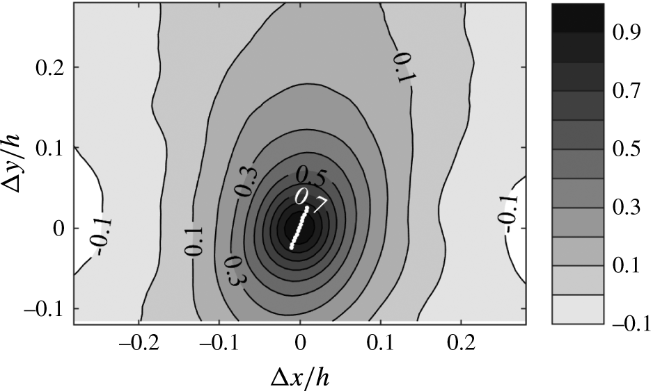
Figure 17. Distribution of two-point correlation of pressure ( $R_{p,p}$ ) for a reference point located at $(0,0.12h,0)$ .

Figure 18. Profile of the average streamwise offset between the pressure at $y_{0}/h=0.12$ and that at other elevations. The values are calculated from the amplitude-weighted argument of pressure–pressure cross-spectrum.

Figure 19. A comparison of the measured streamwise offset of the deformation–pressure correlation peak to that caused by damping only, and the combined effects of hydrodynamic phase lag and material damping. The latter is provided for two values of loss tangent.

Correlations between surface deformation and flow velocity and/or vorticity distributions have been used in efforts aimed at identifying coherent flow structures associated with the wall shape. Here again, trends associated with large positive ( $d>\unicode[STIX]{x1D70E}_{d}$ ) and large negative ( $d<-\unicode[STIX]{x1D70E}_{d}$ ) deformations are displayed and discussed separately. The conditional correlations between wall deformation and three components of the velocity in selected planes are presented in figures 20 and 21. In these plots, the deformation is high-pass filtered at $\unicode[STIX]{x1D714}h/U_{0}=4.3$ , but the velocity is not, to account for effects of structures larger than FOV (further discussion follows). The analysis is performed for all planes and then spatially averaged. In addition to correlations, figures 20 and 21 also show the conditionally averaged projection of streamlines onto the $x{-}y$ and $y{-}z$ planes, respectively, calculated from the corresponding velocity components. The $y{-}z$ planes in figure 21 are presented at two streamwise locations, $\unicode[STIX]{x0394}x/h=0$ , where the deformation is measured, and $\unicode[STIX]{x0394}x/h=0.1$ , which is selected based on the peak of deformation–pressure correlations. In general, all the correlations associated with dimples are higher than those corresponding to bumps. Out of the velocity components, $v^{\prime }$ has the strongest correlation with the wall shape, followed by $u^{\prime }$ and $w^{\prime }$ . For positive deformations, the streamlines and signs of correlations in figure 20(a,c) appear like a swirling flow with preferentially negative $\unicode[STIX]{x1D714}_{z}^{\prime }$ centred at $\unicode[STIX]{x0394}x/h\,\approx \,0.1$ and $\unicode[STIX]{x0394}y/h\,\approx \,0.11$ , very close to the peak of $R_{d,p}|_{d>\unicode[STIX]{x1D70E}d}$ in figure 14(a). Above the deformation, where the correlation values are high, there is a steep ejection-like flow (Q2, with $u^{\prime }<0$ and $v^{\prime }>0$ ). In the correlation maps involving spanwise velocity (figure 21 a,c) the magnitudes are quite low. Based on the streamlines in figure 21(a), and the signs of $R_{d,v}|_{d>\unicode[STIX]{x1D70E}d}$ in figure 20(c), the flow direction above the deformation peak ( $\unicode[STIX]{x0394}x/h=0$ ) is consistent with ‘anti-splatting’, i.e. a flow converging from both spanwise directions and turning upward. Although the signs of $R_{d,w}|_{d>\unicode[STIX]{x1D70E}d}$ at $\unicode[STIX]{x0394}x/h=0$ and $\unicode[STIX]{x0394}x/h=0.1$ are similar, the vertical velocity at the latter is nearly zero.

Figure 20. Conditional deformation–velocity correlations at $(\unicode[STIX]{x0394}x,\unicode[STIX]{x0394}y,\unicode[STIX]{x0394}z=0)$ for positive (a,c) and negative (b,d) deformations: (a) $R_{d,u}|_{d>\unicode[STIX]{x1D70E}d}$ , (b) $R_{d,u}|_{d<-\unicode[STIX]{x1D70E}d}$ , (c) $R_{d,v}|_{d>\unicode[STIX]{x1D70E}d}$ and (d)  $R_{d,v}|_{d<-\unicode[STIX]{x1D70E}d}$ . The streamlines show the corresponding conditionally averaged flow fields.

Figure 21. Conditional deformation–spanwise velocity correlations for positive ( $R_{d,w}|_{d>\unicode[STIX]{x1D70E}d}$ , a,c) and negative ( $R_{d,w}|_{d<-\unicode[STIX]{x1D70E}d}$ , b,d) deformations: (a,b)  $\unicode[STIX]{x0394}x=0$ , bottom row; (c,d)  $\unicode[STIX]{x0394}x=0.1h$ . The streamlines show the corresponding conditionally averaged flow fields.

For negative deformations, both the streamlines and distribution of correlation in figure 20(b,d) show a sweeping flow (Q4, with $u^{\prime }>0$ and $v^{\prime }<0$ ) above the deformation, and a transition between an upstream sweeping flow and a downstream ejection at $\unicode[STIX]{x0394}x/h\approx 0.1$ . The zero-crossing of $R_{d,v}|_{d<-\unicode[STIX]{x1D70E}d}$ at $\unicode[STIX]{x0394}x/h\approx 0.1$ coincides with the streamwise plane of maximum deformation–pressure correlation. The $y{-}z$ plane distribution of $R_{d,w}|_{d<-\unicode[STIX]{x1D70E}d}$ and streamlines at $\unicode[STIX]{x0394}x/h=0$ (figure 21 b) show a splatting flow impinging on the surface and turning outward in the spanwise direction. As shown in figure 22, the magnitude of the $R_{d,u}|_{d>\unicode[STIX]{x1D70E}d}$ and $R_{d,u}|_{d<-\unicode[STIX]{x1D70E}d}$ peaks increase significantly if the conditional correlations are calculated based on high-pass filtered velocity at $\unicode[STIX]{x1D714}h/U_{0}=4.3$ , similar to what is done for the deformation. The same increase occurs for correlations involving the other velocity components (not shown). For $d>\unicode[STIX]{x1D70E}_{d}$ , the dominant phenomenon in the region of peak correlation and above the deformation is an ejection. For $d<-\unicode[STIX]{x1D70E}_{d}$ , the flow direction reverses to a sweep over the same area. Apart from the higher correlation magnitudes, the only appreciable effect of filtering in the spatial distributions is a shift of $R_{d,u}|_{d>\unicode[STIX]{x1D70E}d}$ slightly upstream and away from the wall.

Figure 22. Distributions of conditional deformation–streamwise velocity correlations for high-pass filtered velocity at $\unicode[STIX]{x1D714}h/U_{0}=4.3$ : (a) $R_{d,u}|_{d>\unicode[STIX]{x1D70E}d}$ and (b) $R_{d,u}|_{d<-\unicode[STIX]{x1D70E}d}$ .

Given the connections established between deformation and pressure as well as between deformation and velocity, the ‘loop’ is closed by showing the distributions of conditional pressure–velocity (unfiltered) correlation in figure 23. They are based on the pressure measured at $y_{0}/h=0.12$ , where $\unicode[STIX]{x0394}x=\unicode[STIX]{x0394}y=0$ , and we follow the same procedures described for the deformation–velocity correlations, including spatial averaging over all planes, and calculation of the projection of conditionally averaged streamlines. This elevation is selected in view of the deformation–pressure correlations. To facilitate comparisons with figure 20, panels (a,c) show results for $p<-\unicode[STIX]{x1D70E}_{p}$ , and panels (b,d) correspond to $p>\unicode[STIX]{x1D70E}_{p}$ . The wall-normal velocity component has the strongest correlation with pressure, in agreement with trends reported in Joshi et al. (Reference Joshi, Liu and Katz2014), and consistent with trends of the deformation–velocity correlations. Although the shapes of streamlines differ, in part due to the elevation of the pressure conditioning point, the main flow feature in figure 23 for $p<-\unicode[STIX]{x1D70E}_{p}$ (distributions of $R_{p,u}|_{p<-\unicode[STIX]{x1D70E}p}$ and $R_{p,v}|_{p<-\unicode[STIX]{x1D70E}p}$ and corresponding streamlines) is a large-scale swirl, similar to that observed for $d>\unicode[STIX]{x1D70E}_{d}$ in figure 20, with the streamwise shift noted. In the same manner, the primary phenomenon for $p>\unicode[STIX]{x1D70E}_{p}$ is a saddle point with the flow above it resembling a sweep-ejection transition, consistent with the trends observed for $d<-\unicode[STIX]{x1D70E}_{d}$ . It should be noted that formation of a pressure maximum at the sweep to ejection transition has been observed in several prior studies, e.g. Kim (Reference Kim1983, Reference Kim1989), Kobashi & Ichijo (Reference Kobashi and Ichijo1986), Ghaemi & Scarano (Reference Ghaemi and Scarano2013), Joshi et al. (Reference Joshi, Liu and Katz2014), and Naka et al. (Reference Naka, Stanislas, Foucaut, Coudert, Laval and Obi2015).

Figure 23. The pressure–velocity conditional correlations, based on the pressure at $y=0.12h$ : (a) $R_{p,u}|_{p<-\unicode[STIX]{x1D70E}p}$ , (b) $R_{p,u}|_{p>\unicode[STIX]{x1D70E}p}$ , (c) $R_{p,v}|_{p<-\unicode[STIX]{x1D70E}p}$ , (d) $R_{p,v}|_{p>\unicode[STIX]{x1D70E}p}$ , (e) $R_{p,w}|_{p<-\unicode[STIX]{x1D70E}p}$ and (f)  $R_{p,w}|_{p>\unicode[STIX]{x1D70E}p}$ . In (a–d) $\unicode[STIX]{x0394}z=0$ and in (e,f) $\unicode[STIX]{x0394}x=0$ .

Figure 24. Distributions of pressure–wall-normal velocity conditional correlations on the $\unicode[STIX]{x0394}z=0$ plane, based on the pressure at $(0,0.2h,0)$ : (a) $R_{p,v}|_{p<-\unicode[STIX]{x1D70E}p}$ ; (b) $R_{p,v}|_{p>\unicode[STIX]{x1D70E}p}$ . Streamlines show the corresponding conditionally averaged flow field.

Figure 25. (a,b) Conditional deformation–spanwise vorticity correlations and (c,d) corresponding deformation- $\unicode[STIX]{x1D706}_{2}$ correlations: (a) $R_{d,\unicode[STIX]{x1D714}z^{\prime }}|_{d>\unicode[STIX]{x1D70E}d}$ , (b) $R_{d,\unicode[STIX]{x1D714}z^{\prime }}|_{d<-\unicode[STIX]{x1D70E}d}$ , (c) $R_{d,\unicode[STIX]{x1D706}2}|_{d>\unicode[STIX]{x1D70E}d}$ and (d) $R_{d,\unicode[STIX]{x1D706}2}|_{d<-\unicode[STIX]{x1D70E}d}$ .

There are a few more notable trends. First, for all velocity components, the correlation peaks associated with $p>\unicode[STIX]{x1D70E}_{p}$ are higher than those of $p<-\unicode[STIX]{x1D70E}_{p}$ , also in agreement with corresponding deformation–velocity correlations. Second, the magnitude of the $R_{p,u}|_{p<-\unicode[STIX]{x1D70E}p}$ (figure 23 a) peak is stronger under the ‘vortex’ than that above it, presumably since the horizontal velocity in regions located close to the wall is constructively influenced by the ‘image vortex’ on the other side of the surface. Third, the distribution of $R_{p,w}|_{p<-\unicode[STIX]{x1D70E}p}$ (figure 23 e) depicts an anti-splatting flow, but the magnitudes are low, and that of $R_{p,w}|_{p>\unicode[STIX]{x1D70E}p}$ (figure 23 f) appears like a splatting flow, with correlation magnitudes that are twice as high. The main difference between deformation–velocity and pressure–velocity correlations is the height of the peak. In the deformation–velocity correlations (figure 20), the centre of the swirl for $d>\unicode[STIX]{x1D70E}_{d}$ is located at $\unicode[STIX]{x0394}y/h\sim 0.11$ , whereas the swirl centre for $p<-\unicode[STIX]{x1D70E}_{p}$ and the saddle point at the centre of the $p>\unicode[STIX]{x1D70E}_{p}$ plot shift upward with the pressure conditioning point. For example, figure 24 provides the pressure–wall-normal velocity correlation and conditionally sampled streamlines for pressure measured at $y/h=0.2$ , showing similar flow features shifted to a higher elevation, and an increasing distance between positive and negative correlation peaks. The latter trend is expected due to increase in the size of characteristic eddies with distance from the wall (Townsend Reference Townsend1976; Perry & Chong Reference Perry and Chong1982).

The conditional correlations between deformation and vorticity components have been calculated in order to further characterize flow structures associated with the deformation. Figure 25(a,b) show the deformation–spanwise vorticity correlations conditioned on $d>\unicode[STIX]{x1D70E}_{d}(R_{d,\unicode[STIX]{x1D714}z^{\prime }}|_{d>\unicode[STIX]{x1D70E}d})$ and $d<-\unicode[STIX]{x1D70E}_{d}(R_{d,\unicode[STIX]{x1D714}z^{\prime }}|_{d<-\unicode[STIX]{x1D70E}d})$ , respectively. The peak of $R_{d,\unicode[STIX]{x1D714}z^{\prime }}|_{d>\unicode[STIX]{x1D70E}d}$ is located at $\unicode[STIX]{x0394}x/h\approx 0.1$ and $\unicode[STIX]{x0394}y/h\approx 0.1$ , very close to the centre of the spiral streamlines in figure 20(a,c) and the pressure–deformation correlation peak (figure 14 a). It is characterized by negative correlation values, suggesting that the bump is located preferentially behind/upstream of a region of negative spanwise vorticity fluctuation. To determine whether this vorticity is indeed associated with vortices, we also calculate the distribution of the conditional correlation between deformation and $\unicode[STIX]{x1D706}_{2}$ , which is a popular method for identifying vortices introduced by Jeong & Hussain (Reference Jeong and Hussain1995). Results for $d>\unicode[STIX]{x1D70E}_{d}$ , presented in figure 25(c), show that $\unicode[STIX]{x0394}x/h\approx 0.1$ is characterized by negative values of $\unicode[STIX]{x1D706}_{2}$ , confirming the preferred presence of a vortex. Distributions of $R_{d,\unicode[STIX]{x1D714}z^{\prime }}|_{d>\unicode[STIX]{x1D70E}d}$ in an $x{-}z$ plane for $\unicode[STIX]{x0394}y/h=0.1$ (figure 26 a) indicate the correlation peaks near $\unicode[STIX]{x0394}z=0$ , but it has a broad spanwise extent. Hence, the ejection regions above bumps are preferentially associated with negative spanwise vortices located downstream of the positive deformation. For negative deformations, figure 25(b) shows a region of preferentially positive $\unicode[STIX]{x1D714}_{z}^{\prime }$ , also at $\unicode[STIX]{x0394}x/h\approx 0.1$ and  $\unicode[STIX]{x0394}y/h\approx 0.1$ . However, the corresponding values of $R_{d,\unicode[STIX]{x1D706}2}|_{d<-\unicode[STIX]{x1D70E}d}$ at $\unicode[STIX]{x0394}x/h\sim 0.1$ , which are presented in figure 25(d), are negative. Hence, $\unicode[STIX]{x1D706}_{2}$ is preferentially positive, i.e. the dimples are not associated with the presence of vortices, consistent with the shape of streamlines presented (figure 20). This observation indicates that the $\unicode[STIX]{x1D714}_{z}^{\prime }>0$ region at the sweep-ejection transition around $\unicode[STIX]{x0394}x/h=0.1$ is associated with low vorticity magnitude. It is presumably caused by a decrease in near-wall velocity gradients as the flow is slowing down under the influence of adverse pressure gradients, culminating with separation/ejection. The spanwise extent of this low-velocity-gradient region is broad, as demonstrated by the $x{-}z$ distribution of $R_{d,\unicode[STIX]{x1D714}z^{\prime }}|_{d<-\unicode[STIX]{x1D70E}d}$ presented in figure 26(b).

Figure 26. Conditional deformation–spanwise vorticity correlations in an $x{-}z$ plane located at $\unicode[STIX]{x0394}y/h=0.1$ : (a) $R_{d,\unicode[STIX]{x1D714}z^{\prime }}|_{d>\unicode[STIX]{x1D70E}d}$ ; (b) $R_{d,\unicode[STIX]{x1D714}z^{\prime }}|_{d<-\unicode[STIX]{x1D70E}d}$ .

Figure 27. Conditional deformation–streamwise vorticity correlations in an $x{-}z$ plane located at $\unicode[STIX]{x0394}y/h=0.08$ : (a) $R_{d,\unicode[STIX]{x1D714}x^{\prime }}|_{d>\unicode[STIX]{x1D70E}d}$ ; (b) $R_{d,\unicode[STIX]{x1D714}x^{\prime }}|_{d<-\unicode[STIX]{x1D70E}d}$ .

The conditional correlations between deformation and streamwise vorticity based on large positive ( $R_{d,\unicode[STIX]{x1D714}x^{\prime }}|_{d>\unicode[STIX]{x1D70E}d}$ ) and negative ( $R_{d,\unicode[STIX]{x1D714}x^{\prime }}|_{d<-\unicode[STIX]{x1D70E}d}$ ) deformations are shown in figure 27(a,b), respectively. Results are presented in an $x{-}z$ plane located at $\unicode[STIX]{x0394}y/h=0.08$ , which is the elevation where the correlation magnitudes peak. Distributions in other nearby elevations have similar shapes (not shown). In both cases, correlation extrema with low magnitudes are preferentially located in a different spanwise plane relative to the deformation conditioning point. The two correlation peaks with opposite signs at $-0.1<\unicode[STIX]{x0394}x/h<0.1$ in figure 27(a) indicate that bumps are preferentially developed in regions where the streamwise-vortex-induced wall-normal velocity is positive (ejections). Further downstream, at $\unicode[STIX]{x0394}x/h>0.1$ , the correlation extrema have opposite signs, consistent with a sweeping motion. As demonstrated later, and consistent with the spanwise vortex at $\unicode[STIX]{x0394}x/h\sim 0.1$ (figures 25 a and 26 a), the bumps preferentially form under and upstream of the head of a hairpin vortex.

Figure 28. (a–c) Results of analysis conditioned on $d(0,0)>\unicode[STIX]{x1D70E}_{d}$ and $\unicode[STIX]{x1D714}_{x}^{\prime }(0,0.08h,0.05h)>0$ : (a) $d$ – $\unicode[STIX]{x1D714}_{x}^{\prime }$ correlation in the $\unicode[STIX]{x0394}z/h=0.05$ plane; (b) $d$ – $\unicode[STIX]{x1D714}_{z}^{\prime }$ correlation at $\unicode[STIX]{x0394}z/h=0$ ; (c) iso-surfaces of $\overline{\unicode[STIX]{x1D714}_{x}^{\prime }h/U_{0}}=-0.17$ , $=0.25$ and $\overline{\unicode[STIX]{x1D714}_{z}^{\prime }h/U_{0}}=-0.20$ , along with the corresponding vortex lines; and (d) pressure–spanwise vorticity correlation conditioned on $p<-\unicode[STIX]{x1D70E}_{p}$ (at $y=0.12h$ , as indicated by a $+$ ) in the $\unicode[STIX]{x0394}z=0$ plane.

This relationship between $\unicode[STIX]{x1D714}_{x}^{\prime }$ , $\unicode[STIX]{x1D714}_{z}^{\prime }$ , and positive deformation is further investigated by calculating the deformation–vorticity correlations, conditioned on both $d(0,0)>\unicode[STIX]{x1D70E}_{d}$ , and $\unicode[STIX]{x1D714}_{x}^{\prime }(0,0.08h,0.05h)>0$ . Results for $d$ – $\unicode[STIX]{x1D714}_{x}^{\prime }$ correlation in the $\unicode[STIX]{x0394}z/h=0.05$ plane is presented in figure 28(a), and that for $d$ – $\unicode[STIX]{x1D714}_{z}^{\prime }$ in the $\unicode[STIX]{x0394}z/h=0$ plane in figure 28(b). The vertical coordinates are expressed both in terms of $\unicode[STIX]{x0394}y/h$ and $y/h$ . The fact that the $d$ – $\unicode[STIX]{x1D714}_{x}^{\prime }$ correlation peaks at the conditioning point is not meaningful because the positive values are imposed. However, figure 28(a) also shows an inclined layer of elevated correlations extending from both sides of the peak having the familiar angle of $15^{\circ }$ – $20^{\circ }$ (exact value depends on the criterion used) with the horizontal direction. The same angle has been seen for $R_{u,u}$ in many studies (e.g. Kim Reference Kim1989; Liu, Adrian & Hanratiy Reference Liu, Adrian and Hanratiy2001; Hutchins & Marusic Reference Hutchins and Marusic2007b ; Wu & Christensen Reference Wu and Christensen2010; Ghaemi & Scarano Reference Ghaemi and Scarano2013; Sillero, Jiménez & Moser Reference Sillero, Jiménez and Moser2014), and have been attributed to hairpin vortices (Adrian, Meinhart & Tomkins Reference Adrian, Meinhart and Tomkins2000). Furthermore, figure 28(b) shows a region of high correlation with negative spanwise vorticity downstream, above and spanwise offset from the $\unicode[STIX]{x1D714}_{x}^{\prime }$ conditioning point. The elevation of this peak, $y/h\,=\,0.13$ , falls within the broad minimum in figure 25(a) (both are conditioned on $d>\unicode[STIX]{x1D70E}_{d}$ ), but adding the offset $\unicode[STIX]{x1D714}_{x}^{\prime }$ constraint increases the $d$ – $\unicode[STIX]{x1D714}_{z}^{\prime }$ correlation peak magnitude by ${\sim}100\,\%$ . Hence, the elevated $d$ – $\unicode[STIX]{x1D714}_{x}^{\prime }$ correlation appears to be a leg of a hairpin vortex, and the $d$ – $\unicode[STIX]{x1D714}_{z}^{\prime }$ correlation peak is the head of this vortex. Additional confirmation can be obtained by plotting the conditionally averaged flow field under the same conditions. Figure 28(c) shows iso-surfaces of $\overline{\unicode[STIX]{x1D714}_{x}^{\prime }h/U_{0}}=-0.17$ and 0.25, as well as $\overline{\unicode[STIX]{x1D714}_{z}^{\prime }h/U_{0}}=-0.2$ in different colours (overbar indicates conditionally averaged variable). It confirms the preferred presence of an inclined quasi-streamwise vortex as well as a counter-rotating (negative) vortex on the other side of the deformation, located at a distance of $\unicode[STIX]{x0394}z=0.15h(\unicode[STIX]{x0394}z^{+}=350)$ from the conditioning point. It also shows the region with high $\overline{\unicode[STIX]{x1D714}_{z}^{\prime }h/U_{0}}$ at the head of the hairpin. Finally, figure 28(c) also shows several conditionally averaged vortex lines originating from the vicinity of the vorticity conditioning point, passing through the hairpin head, and turning back into the other leg. Clearly, the positive deformation is located upstream of a negative spanwise vortex and flanked by streamwise vortices of opposite signs, consistent with the features of a hairpin-like structure. If the analysis is repeated by imposing $\unicode[STIX]{x1D714}_{x}^{\prime }(0,0.08h,-0.05h)<0$ , the 3D depiction appears to be quite similar (not shown) except for a swap in the size of the iso-surfaces of $\overline{\unicode[STIX]{x1D714}_{x}^{\prime }h/U_{0}}$ , corresponding to the location of the conditioning point. The picture becomes complete by plotting the distribution of pressure–spanwise vorticity correlation, conditioned on $p(0,0.12h,0)<-\unicode[STIX]{x1D70E}_{p}$ in figure 28(d). It shows that the pressure minimum is located in the same streamwise plane but slightly below the negative spanwise vorticity peak, and falls within the broad deformation–pressure correlation peak in figure 14(a). Hence, the pressure minimum preferentially causing the bump upstream of the hairpin head is located slightly below the point of peak spanwise vorticity. Such a vertical offset between the locations of pressure and spanwise vorticity minima in a hairpin structure is consistent with trends reported by Ghaemi & Scarano (Reference Ghaemi and Scarano2013). Their measurements focus on the $y^{+}<149$ region, and show a distance of $\unicode[STIX]{x0394}z^{+}\approx 80$ between the hairpin legs, and the present observations extend to higher elevation with the corresponding larger distance between legs.

For negative deformations, we have already established that there is no spanwise vortex in front of dimples in the vicinity of the $d$ – $\unicode[STIX]{x1D714}_{z}^{\prime }$ correlation peak (figure 25 b,d). The pressure maximum causing this dimple is preferentially associated with a transition between sweep and ejection (figure 23 b,d). The positive spanwise vorticity fluctuation ahead of the dimple is located in the ejection region, where the averaged vorticity is lower than the mean (negative) value. As illustrated in numerous papers, for example, Kim (Reference Kim1983, Reference Kim1989), Kobashi & Ichijo (Reference Kobashi and Ichijo1986), Chang, Piomelli & Blake (Reference Chang, Piomelli and Blake1999), Ghaemi & Scarano (Reference Ghaemi and Scarano2013), Joshi et al. (Reference Joshi, Liu and Katz2014) and Naka et al. (Reference Naka, Stanislas, Foucaut, Coudert, Laval and Obi2015), an inclined shear layer forms at the interface between an upstream sweep to a downstream ejection. The vicinity of the origin of this layer is shown in figures 20(b) and 23(b), and a more extended view is evident from the conditionally average pressure distribution and streamlines presented in figure 29 for $p(0,0.02h,0)>\unicode[STIX]{x1D70E}_{p}$ . Inclination of this shear layer might be contributing to the (hydrodynamically induced) streamwise phase lag between dimples and the positive pressure fluctuations at $y/h>0.12$ , the location of peak correlation (figure 14 c,d). In addition, the correlation peaks at $-0.1<\unicode[STIX]{x0394}x/h<0.1$ in figure 27(b) indicate that dimples preferentially form in regions with streamwise-vortex-induced downward sweeping flows. Such a phenomenon is not necessarily associated with sweep-ejection transition. However, as figure 27(b) shows, the deformation–streamwise vorticity correlation sign changes at $\unicode[STIX]{x0394}x/h>0.1$ . Such a change might occur, for example, at a sweep-ejection transition, where the direction of velocity fluctuation changes abruptly.

Figure 29. The conditionally averaged pressure distribution and streamlines, based on $p(0,0.02h,0)>\unicode[STIX]{x1D70E}_{p}$ .