


1. Introduction
How do people make perceptual judgments based on the available sensory information? This fundamental question has been a focus of psychological research from the nineteenth century onward (Fechner Reference Fechner1860; Helmholtz Reference Helmholtz1856). Many perceptual tasks naturally lend themselves to what has traditionally been called “ideal observer” analysis, whereby the optimal behavior is mathematically determined given a set of assumptions such as the presence of sensory noise, and human behavior is compared to this standard (Geisler Reference Geisler2011; Green & Swets Reference Green and Swets1966; Ulehla Reference Ulehla1966). The extensive literature on this topic includes many examples of humans performing similarly to an ideal observer but also many examples of suboptimal behavior. Perceptual science has a strong tradition of developing models and theories that attempt to account for the full range of empirical data on how humans perceive (Macmillan & Creelman Reference Macmillan and Creelman2005).
Recent years have seen an impressive surge of Bayesian theories of human cognition and perception (Gershman et al. Reference Gershman, Horvitz and Tenenbaum2015; Griffiths et al. Reference Griffiths, Lieder and Goodman2015; Tenenbaum et al. Reference Tenenbaum, Kemp, Griffiths and Goodman2011). These theories often depict humans as optimal decision makers, especially in the area of perception. А number of high-profile papers have shown examples of human perceptual behavior that is close to optimal (Ernst & Banks Reference Ernst and Banks2002; Körding & Wolpert Reference Körding and Wolpert2004; Landy et al. Reference Landy, Maloney, Johnston and Young1995; Shen & Ma Reference Shen and Ma2016), whereas other papers have attempted to explain apparently suboptimal behaviors as being in fact optimal (Weiss et al. Reference Weiss, Simoncelli and Adelson2002). Consequently, many statements by researchers in the field leave the impression that humans are essentially optimal in perceptual tasks:
Psychophysics is providing a growing body of evidence that human perceptual computations are “Bayes’ optimal.” (Knill & Pouget Reference Knill and Pouget2004, p. 712)
Across a wide range of tasks, people seem to act in a manner consistent with optimal Bayesian models. (Vul et al. Reference Vul, Goodman, Griffiths and Tenenbaum2014, p. 1)
These studies with different approaches have shown that human perception is close to the Bayesian optimal. (Körding & Wolpert Reference Körding and Wolpert2006, p. 321)
Despite a number of recent criticisms of such assertions regarding human optimality (Bowers & Davis Reference Bowers and Davis2012a; Reference Bowers and Davis2012b; Eberhardt & Danks Reference Eberhardt and Danks2011; Jones & Love Reference Jones and Love2011; Marcus & Davis Reference Marcus and Davis2013; Reference Marcus and Davis2015), as well as statements from some of the most prominent Bayesian theorists that their goal is not to demonstrate optimality (Goodman et al. Reference Goodman, Frank, Griffiths, Tenenbaum, Battaglia and Hamrick2015; Griffiths et al. Reference Griffiths, Chater, Norris and Pouget2012), the previous quotes indicate that the view that humans are (close to) optimal when making perceptual decisions has taken a strong foothold.
The main purpose of this article is to counteract assertions about human optimality by bringing together the extensive literature on suboptimal perceptual decision making. Although the description of the many findings of suboptimality will occupy a large part of the article, we do not advocate for a shift of labeling observers from “optimal” to “suboptimal.” Instead, we will ultimately argue that we should abandon any emphasis on optimality or suboptimality and return to building a science of perception that attempts to account for all types of behavior.
The article is organized into six sections. After introducing the topic (sect. 1), we explain the Bayesian approach to perceptual decision making and explicitly define a set of standard assumptions that typically determine what behavior is considered optimal (sect. 2). In the central section of the article, we review the vast literature of suboptimal perceptual decision making and show that suboptimalities have been reported in virtually every class of perceptual tasks (sect. 3). We then discuss theoretical problems with the current narrow focus on optimality, such as difficulties in defining what is truly optimal and the limited value of optimality claims in and of themselves (sect. 4). Finally, we argue that the way forward is to build observer models that give equal emphasis to all components of perceptual decision making, not only the decision rule (sect. 5). We conclude that the field should abandon its emphasis on optimality and instead focus on thoroughly testing the hypotheses that have already been generated (sect. 6).
2. Defining optimality
Optimality can be defined within many frameworks. Here we adopt a Bayesian approach because it is widely used in the field and it is general: other approaches to optimality can often be expressed in Bayesian terms.
2.1. The Bayesian approach to perceptual decision making
The Bayesian approach to perceptual decision making starts with specifying the generative model of the task. The model defines the sets of world states, or stimuli,  ${\rm {\cal S}}$, internal responses
  ${\rm {\rm X}}$, actions
  ${\rm {\cal A}}$, and relevant parameters Θ (such as the sensitivity of the observer). We will mostly focus on cases in which two possible stimuli s 1 and s 2 are presented, and the possible “actions” a 1 and a 2 are reporting that the corresponding stimulus was shown. The Bayesian approach then specifies the following quantities (see Fig. 1 for a graphical depiction):
Likelihood function. An external stimulus can produce a range of internal responses. The measurement density, or distribution, p(x|s, θ) is the probability density of obtaining an internal response x given a particular stimulus s. The likelihood function l(s|x, θ) is equal to the measurement density but is defined for a fixed internal response as opposed to a fixed stimulus.
Prior. The prior π(s) describes one's assumptions about the probability of each stimulus s.
Cost function. The cost function
 ${\rm \;\ {\cal L}}\lpar {s,a} \rpar $ (also called loss function) specifies the cost of taking a specific action for a specific stimulus.
Decision rule. The decision rule δ(x) indicates under what combination of the other quantities you should perform one action or another.


Figure 1. Graphical depiction of Bayesian inference. An observer is deciding between two possible stimuli – s 1 (e.g., leftward motion) and s 2 (e.g., rightward motion) – which produce Gaussian measurement distributions of internal responses. The observer's internal response varies from trial to trial, depicted by the three yellow circles for three example trials. On a given trial, the likelihood function is equal to the height of each of the two measurement densities at the value of the observed internal response (lines drawn from each yellow circle) – that is, the likelihood of each stimulus given an internal response. For illustrative purposes, a different experimenter-provided prior and cost function are assumed on each trial. The action a i corresponds to choosing stimulus s i. We obtain the expected cost of each action by multiplying the likelihood, prior, and cost corresponding to each stimulus and then summing the costs associated with the two possible stimuli. The optimal decision rule is to choose the action with the lower cost (the bar with less negative values). In trial 1, the prior and cost function are unbiased, so the optimal decision depends only on the likelihood function. In trial 2, the prior is biased toward s 2, making a 2 the optimal choice even though s 1 is slightly more likely. In trial 3, the cost function favors a 1, but the much higher likelihood of s 2 makes a 2 the optimal choice.
We refer to the likelihood function, prior, cost function, and decision rule as the LPCD components of perceptual decision making.
According to Bayesian decision theory (Körding & Wolpert Reference Körding and Wolpert2006; Maloney & Mamassian Reference Maloney and Mamassian2009), the optimal decision rule is to choose the action a that minimizes the expected loss over all possible stimuli. Using Bayes’ theorem, we can derive the optimal decision rule as a function of the likelihood, prior, and cost function:
 $$\delta \lpar x \rpar = {\rm argmin}_{a\in A}\mathop \sum \limits_{s\in {\rm {\cal S}}} l(s \vert x,\theta ){\rm \;} \pi \lpar s \rpar {\rm \;\ {\cal L}}\lpar {s,a} \rpar. $$
2.2. Standard assumptions
Determining whether observers’ decisions are optimal requires the specification of the four LPCD components. How do researchers determine the quantitative form of each component? The following is a typical set of standard assumptions related to each LPCD component:
Likelihood function assumptions. The standard assumptions here include Gaussian measurement distributions and stimulus encoding that is independent from other factors such as stimulus presentation history. Note that the experimenter derives the likelihood function from the assumed measurement distributions.
Prior and cost function assumptions. The standard assumption about observers’ internal representations of the prior and cost function is that they are identical to the quantities defined by the experimenter. Unless specifically mentioned, the experiments reviewed subsequently here present s 1 and s 2 equally often, which is equivalent to a uniform prior (e.g.,
$\pi \lpar {s_i} \rpar = \; \displaystyle{1 \over 2}$ when there are two stimuli), and expect observers to maximize percent correct, which is equivalent to a cost function that punishes all incorrect responses, and rewards all correct responses, equally.Decision rule assumptions. The standard assumption about the decision rule is that it is identical to the optimal decision rule.

Finally, additional general standard assumptions include expectations that observers can perform the proper computations on the LPCD components. Note that as specified, the standard assumptions consider Gaussian variability at encoding as the sole corrupting element for perceptual decisions. Section 3 assembles the evidence against this claim.
The attentive reader may object that the standard assumptions cannot be universally true. For example, assumptions related to the likelihood function are likely false for specific paradigms (e.g., measurement noise may not be Gaussian), and assumptions about observers adopting the experimentally defined prior and cost function are likely false for complex experimental designs (Beck et al. Reference Beck, Ma, Pitkow, Latham and Pouget2012). Nevertheless, we take the standard assumptions as a useful starting point for our review because, explicitly or implicitly, they are assumed in most (although not all) studies. In section 3, we label all deviations from behavior prescribed by the standard assumptions as examples of suboptimality. We discuss alternative ways of defining optimality in section 4 and ultimately argue that general statements about the optimality or suboptimality of perceptual decisions are meaningless.
3. Review of suboptimality in perceptual decision making
We review eight categories of tasks for which the optimal decision rule can be determined. For each task category, we first note any relevant information about the measurement distribution, prior, or cost function. We plot the measurement distributions together with the optimal decision rule (which we depict as a criterion drawn on the internal responses  ${\rm {\rm X}}$). We then review specific suboptimalities within each task category. For each explanation of apparently suboptimal behavior, we indicate the standard LPCD components proposed to have been violated using the notation [LPCD component], such as [decision rule]. Note that violations of the assumed measurement distributions result in violations of the assumed likelihood functions. In some cases, suboptimalities have been attributed to issues that apply to multiple components (indicated as [general]) or issues of methodology (indicated as [methodological]).
3.1. Criterion in two-choice tasks
In the most common case, observers must distinguish between two possible stimuli, s 1 and s 2, presented with equal probability and associated with equal reward. In Figure 2, we plot the measurement distributions and optimal criteria for the cases of equal and unequal internal variability. The criterion used to make the decision corresponds to the decision rule.
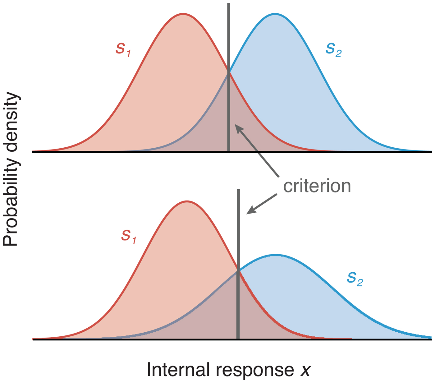
Figure 2. Depiction of the measurement distributions (colored curves) and optimal criteria (equivalent to the decision rules) in two-choice tasks. The upper panel depicts the case when the two stimuli produce the same internal variability (σ 1 = σ 2, where σ is the standard deviation of the Gaussian measurement distribution). The gray vertical line represents the location of the optimal criterion. The lower panel shows the location of the optimal criterion when the variability of the two measurement distributions differs (σ 1 < σ 2, in which case the optimal criterion results in a higher proportion of s 1 responses).
3.1.1. Detection criteria
Many tasks involve the simple distinction between noise (s1) and signal + noise (s2). These are usually referred to as detection tasks. In most cases, s1 is found to produce smaller internal variability than s2 (Green & Swets Reference Green and Swets1966; Macmillan & Creelman Reference Macmillan and Creelman2005; Swets et al. Reference Swets, Tanner and Birdsall1961), from which it follows that an optimal observer would choose s1 more often than s2 even when the two stimuli are presented at equal rates (Fig. 2). Indeed, many detection studies find that observers choose the noise distribution s1 more than half of the time (Gorea & Sagi Reference Gorea and Sagi2000; Green & Swets Reference Green and Swets1966; Rahnev et al. Reference Rahnev, Maniscalco, Graves, Huang, de Lange and Lau2011b; Reckless et al. Reference Reckless, Ousdal, Server, Walter, Andreassen and Jensen2014; Solovey et al. Reference Solovey, Graney and Lau2015; Swets et al. Reference Swets, Tanner and Birdsall1961). However, most studies do not allow for the estimation of the exact measurement distributions for individual observers, and hence it is an open question how optimal observers in those studies actually are. A few studies have reported conditions in which observers choose the noise stimulus s1 less than half of the time (Morales et al. Reference Morales, Solovey, Maniscalco, Rahnev, de Lange and Lau2015; Rahnev et al. Reference Rahnev, Maniscalco, Graves, Huang, de Lange and Lau2011b; Solovey et al. Reference Solovey, Graney and Lau2015). Assuming that the noise distributions in those studies also had lower variability, such behavior is likely suboptimal.
3.1.2. Discrimination criteria
Detection tasks require observers to distinguish between the noise versus signal + noise stimuli, but other tasks require observers to discriminate between two roughly equivalent stimuli. For example, observers might discriminate leftward versus rightward motion or clockwise versus counterclockwise grating orientation. For these types of stimuli, the measurement distributions for each stimulus category can be assumed to have approximately equal variability (Macmillan & Creelman Reference Macmillan and Creelman2005; See et al. Reference See, Warm, Dember and Howe1997). Such studies find that the average criterion location across the whole group of observers is usually close to optimal, but individual observers can still exhibit substantial biases (e.g., Whiteley & Sahani, Reference Whiteley and Sahani2008). In other words, what appears as an optimal criterion on average (across observers) may be an average of suboptimal criteria (Mozer et al. Reference Mozer, Pashler and Homaei2008; Vul et al. Reference Vul, Goodman, Griffiths and Tenenbaum2014). This issue can appear within an individual observer, too, with suboptimal criteria on different trials averaging out to resemble an optimal criterion (see sect. 3.2). To check for criterion optimality within individual observers, we re-analyzed the data from a recent study in which observers discriminated between a grating tilted 45 degrees clockwise or counterclockwise from vertical (Rahnev et al. Reference Rahnev, Nee, Riddle, Larson and D'Esposito2016). Seventeen observers came for four sessions on different days completing 480 trials each time. Using a binomial test, we found that 57 of the 68 total sessions exhibited significant deviation from unbiased responding. Further, observers tended to have relatively stable biases as demonstrated by a positive criterion correlation across all pairs of sessions (all p's < .003). Hence, even if the performance of the group appears to be close to optimal, individual observers may deviate substantially from optimality.
3.1.3. Two-stimulus tasks
The biases observed in detection and discrimination experiments led to the development of the two-alternative forced-choice (2AFC) task, in which both stimulus categories are presented on each trial (Macmillan & Creelman Reference Macmillan and Creelman2005). The 2AFC tasks separate the two stimuli either temporally (also referred to as two-interval forced-choice or 2IFC tasks) or spatially. Note that, in recent years, researchers have begun to use the term “2AFC” for two-choice tasks in which only one stimulus is presented. To avoid confusion, we adopt the term “two-stimulus tasks” to refer to tasks where two stimuli are presented (the original meaning of 2AFC) and the term “one-stimulus tasks” to refer to tasks like single-stimulus detection and discrimination (e.g., the tasks discussed in sects. 3.1.1 and 3.1.2).
Even though two-stimulus tasks were designed to remove observer bias, significant biases have been observed for them, too. Although biases in spatial 2AFC tasks have received less attention, several suboptimalities have been documented for 2IFC tasks. For example, early research suggested that the second stimulus is more often selected as the one of higher intensity, a phenomenon called time-order errors (Fechner Reference Fechner1860; Osgood Reference Osgood1953). More recently, Yeshurun et al. (Reference Yeshurun, Carrasco and Maloney2008) re-analyzed 2IFC data from 17 previous experiments and found significant interval biases. The direction of the bias varied across the different experiments, suggesting that the specific experimental design has an influence on observers’ bias.
3.1.4. Explaining suboptimality in two-choice tasks
Why do people appear to have trouble setting appropriate criteria in two-choice tasks? One possibility is that they have a tendency to give the same fixed response when uncertain [decision rule]. For example, a given observer may respond that he saw left (rather than right) motion every time he got distracted or had very low evidence for either choice. This could be because of a preference for one of the two stimuli or one of the two motor responses. Re-analysis of another previous study (Rahnev et al. Reference Rahnev, Lau and de Lange2011a), where we withheld the stimulus-response mapping until after the stimulus presentation, found that 12 of the 21 observers still showed a significant response bias for motion direction. Therefore, a preference in motor behavior cannot fully account for this type of suboptimality.
Another possibility is that for many observers even ostensibly “equivalent” stimuli such as left and right motion give rise to measurement distributions with unequal variance [likelihood function]. In that case, an optimal decision rule would produce behavior that appears biased. Similarly, in two-stimulus tasks, it is possible that the two stimuli are not given the same resources or that the internal representations for each stimulus are not independent of each other [likelihood function]. Finally, in the case of detection tasks, it is possible that some observers employ an idiosyncratic cost function by treating misses as less costly than false alarms because the latter can be interpreted as lying [cost function].
3.2. Maintaining stable criteria
So far, we have considered the optimality of the decision rule when all trials are considered together. We now turn our attention to whether observers’ decision behavior varies across trials or conditions (Fig. 3).

Figure 3. Depiction of a failure to maintain a stable criterion. The optimal criterion is shown in Figure 2, but observers often fail to maintain that criterion over the course of the experiment, resulting in a criterion that effectively varies across trials. Colored curves show measurement distributions.
3.2.1. Sequential effects
Optimality in laboratory tasks requires that judgments are made based on the evidence from the current stimulus independent of previous stimuli. However, sequential effects are ubiquitous in perceptual tasks (Fischer & Whitney Reference Fischer and Whitney2014; Fründ et al. Reference Frund, Wichmann and Macke2014; Kaneko & Sakai Reference Kaneko and Sakai2015; Liberman et al. Reference Liberman, Fischer and Whitney2014; Norton et al. Reference Norton, Fleming, Daw and Landy2017; Tanner et al. Reference Tanner, Haller and Atkinson1967; Treisman & Faulkner Reference Treisman and Faulkner1984; Ward & Lockhead Reference Ward and Lockhead1970; Yu & Cohen Reference Yu, Cohen, Koller, Schuurmans, Bengio and Bottou2009). The general finding is that observers’ responses are positively autocorrelated such that the response on the current trial is likely to be the same as on the previous trial, though in some cases negative autocorrelations have also been reported (Tanner et al. Reference Tanner, Haller and Atkinson1967; Ward & Lockhead Reference Ward and Lockhead1970). Further, observers are able to adjust to new trial-to-trial statistics, but this adjustment is only strong in the direction of default biases and weak in the opposite direction (Abrahamyan et al. Reference Abrahamyan, Luz Silva, Dakin, Carandini and Gardner2016). Similar effects have been observed in other species such as mice (Busse et al. Reference Busse, Ayaz, Dhruv, Katzner, Saleem, Schölvinck, Zaharia and Carandini2011).
3.2.2. Criterion attraction
Interleaving trials that require different criteria also hinders optimal criterion placement. Gorea and Sagi (Reference Gorea and Sagi2000) proposed that when high-contrast stimuli (optimally requiring a relatively conservative detection criterion) and low-contrast stimuli (optimally requiring a relatively liberal detection criterion) were presented simultaneously, observers used the same compromised detection criterion that was suboptimal for both the high- and low-contrast stimuli. This was despite the fact that, on each trial, they told observers with 100% certainty which contrasts might have been present in each location. Similar criterion attraction has been proposed in a variety of paradigms that involved using stimuli of different contrasts (Gorea & Sagi Reference Gorea and Sagi2001; Reference Gorea and Sagi2002; Gorea et al. Reference Gorea, Caetta and Sagi2005; Zak et al. Reference Zak, Katkov, Gorea and Sagi2012), attended versus unattended stimuli (Morales et al. Reference Morales, Solovey, Maniscalco, Rahnev, de Lange and Lau2015; Rahnev et al. Reference Rahnev, Maniscalco, Graves, Huang, de Lange and Lau2011b), and central versus peripheral stimuli (Solovey et al. Reference Solovey, Graney and Lau2015). Although proposals of criterion attraction consider the absolute location of the criterion on the internal decision axis, recent work has noted the methodological difficulties of recovering absolute criteria in signal detection tasks (Denison et al. Reference Denison, Adler, Carrasco and Ma2018).
3.2.3. Irrelevant reward influencing the criterion
The optimal decision rule is insensitive to multiplicative changes to the cost function. For example, rewarding all correct responses with $0.01 versus $0.03, while incorrect responses receive $0, should not alter the decision criterion; in both cases, the optimal decision rule is the one that maximizes percent correct. However, greater monetary rewards or punishments lead observers to adopt a more liberal detection criterion such that more stimuli are identified as targets (Reckless et al. Reference Reckless, Bolstad, Nakstad, Andreassen and Jensen2013; Reference Reckless, Ousdal, Server, Walter, Andreassen and Jensen2014). Similar changes to the response criterion because of monetary motivation are obtained in a variety of paradigms (Henriques et al. Reference Henriques, Glowacki and Davidson1994; Taylor et al. Reference Taylor, Welsh, Wagner, Phan, Fitzgerald and Gehring2004). To complicate matters, observers’ personality traits interact with the type of monetary reward in altering response criteria (Markman et al. Reference Markman, Baldwin and Maddox2005).
3.2.4. Explaining suboptimality in maintaining stable criteria
Why do people appear to shift their response criteria based on factors that should be irrelevant for criterion placement? Sequential effects are typically explained in terms of an automatic tendency to exploit the continuity in our normal environment, even though such continuity is not present in most experimental setups (Fischer & Whitney Reference Fischer and Whitney2014; Fritsche et al. Reference Fritsche, Mostert and de Lange2017; Liberman et al. Reference Liberman, Fischer and Whitney2014). The visual system could have built-in mechanisms that bias new representations toward recent ones [likelihood function], or it may assume that a new stimulus is likely to be similar to a recent one [prior]. (Note that the alternative likelihoods or priors would need to be defined over pairs or sequences of trials.) Adopting a prior that the environment is autocorrelated may be a good strategy for maximizing reward: Environments typically are autocorrelated and, if they are not, such a prior may not hurt performance (Yu & Cohen Reference Yu, Cohen, Koller, Schuurmans, Bengio and Bottou2009).
Criterion attraction may stem from difficulty maintaining two separate criteria simultaneously. This is equivalent to asserting that in certain situations observers cannot maintain a more complicated decision rule (e.g., different criteria for different conditions) and instead use a simpler one (e.g., single criterion for all conditions) [decision rule]. It is harder to explain why personality traits or task features such as increased monetary rewards (that should be irrelevant to the response criterion) change observers’ criteria.
3.3. Adjusting choice criteria
Two of the most common ways to assess optimality in perceptual decision making are to manipulate the prior probabilities of the stimulus classes and to provide unequal payoffs that bias responses toward one of the stimulus categories (Macmillan & Creelman Reference Macmillan and Creelman2005). Manipulating prior probabilities affects the prior π(s), whereas manipulating payoffs affects the cost function  ${\rm {\cal L}}\lpar {s,a} \rpar $. However, the two manipulations have an equivalent effect on the optimal decision rule: Both require observers to shift their decision criterion by a factor dictated by the specific prior probability or reward structure (Fig. 4).
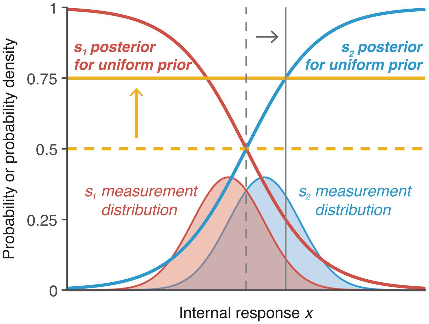
Figure 4. Depiction of optimal adjustment of choice criteria. In addition to the s 1 and s 2 measurement distributions (in thin red and blue lines), the figure shows the corresponding posterior probabilities as a function of x assuming uniform prior (in thick red and blue lines). The vertical criteria depict optimal criterion locations on x (thin gray lines) and correspond to the horizontal thresholds (thick yellow lines). Optimal criterion and threshold for equal prior probabilities and payoffs are shown in dashed lines. If unequal prior probability or unequal payoff is provided such that s 1 ought to be chosen three times as often as s 2, then the threshold would optimally be shifted to 0.75, corresponding to a shift in the criterion such that the horizontal threshold and vertical criterion intersect on the s 2 posterior probability function. The y-axis is probability density for the measurement distributions and probability for the posterior probability functions; the y-axis ticks refer to the posterior probability.
3.3.1. Priors
Two main approaches have been used to determine whether observers can optimally adjust their criterion when one of two stimuli has a higher probability of occurrence. In base-rate manipulations, long blocks of the same occurrence frequency are employed, and observers are typically not informed of the probabilities of occurrence in advance (e.g., Maddox Reference Maddox1995). Most studies find that observers adjust their criterion to account for the unequal base rate, but this adjustment is smaller than what is required for optimal performance, resulting in a conservative criterion placement (Bohil & Maddox Reference Bohil and Maddox2003b; Green & Swets Reference Green and Swets1966; Maddox & Bohil Reference Maddox and Bohil2001; Reference Maddox and Bohil2003; Reference Maddox and Bohil2005; Maddox & Dodd Reference Maddox and Dodd2001; Maddox et al. Reference Maddox, Bohil and Dodd2003; Tanner Reference Tanner1956; Tanner et al. Reference Tanner, Haller and Atkinson1967; Vincent Reference Vincent2011). Some studies have suggested that observers become progressively more suboptimal as the base rate becomes progressively more extreme (Bohil & Maddox Reference Bohil and Maddox2003b; Green & Swets Reference Green and Swets1966). However, a few studies have reported that certain conditions result in extreme criterion placement such that observers rely more on base rate information than is optimal (Maddox & Bohil Reference Maddox and Bohil1998b).
A second way to manipulate the probability of occurrence is to do it on a trial-by-trial basis and explicitly inform observers about the stimulus probabilities before each trial. This approach also leads to conservative criterion placement such that observers do not shift their criterion enough (Ackermann & Landy Reference Ackermann and Landy2015; de Lange et al. Reference de Lange, Rahnev, Donner and Lau2013; Rahnev et al. Reference Rahnev, Lau and de Lange2011a; Summerfield & Koechlin Reference Summerfield and Koechlin2010; Ulehla Reference Ulehla1966).
3.3.2. Payoffs
The decision criterion can also be manipulated by giving different payoffs for different responses. The general finding with this manipulation is that observers, again, do not adjust their criterion enough (Ackermann & Landy Reference Ackermann and Landy2015; Bohil & Maddox Reference Bohil and Maddox2001; Reference Bohil and Maddox2003a; Reference Bohil and Maddox2003b; Busemeyer & Myung Reference Busemeyer and Myung1992; Maddox & Bohil Reference Maddox and Bohil1998a; Reference Maddox and Bohil2000; Reference Maddox and Bohil2001; Reference Maddox and Bohil2003; Reference Maddox and Bohil2005; Maddox & Dodd Reference Maddox and Dodd2001; Maddox et al. Reference Maddox, Bohil and Dodd2003; Markman et al. Reference Markman, Baldwin and Maddox2005; Taylor et al. Reference Taylor, Welsh, Wagner, Phan, Fitzgerald and Gehring2004; Ulehla Reference Ulehla1966) and, as with base rates, become more suboptimal for more extreme payoffs (Bohil & Maddox Reference Bohil and Maddox2003b). Nevertheless, one study that involved a very large number of sessions with two monkeys reported extreme criterion changes (Feng et al. Reference Feng, Holmes, Rorie and Newsome2009).
Criterion adjustments in response to unequal payoffs are usually found to be more suboptimal compared with adjustments in response to unequal base rates (Ackermann & Landy Reference Ackermann and Landy2015; Bohil & Maddox Reference Bohil and Maddox2001; Reference Bohil and Maddox2003a; Busemeyer & Myung Reference Busemeyer and Myung1992; Healy & Kubovy Reference Healy and Kubovy1981; Maddox Reference Maddox2002; Maddox & Bohil Reference Maddox and Bohil1998a; Maddox & Dodd Reference Maddox and Dodd2001), though the opposite pattern was found by Green and Swets (Reference Green and Swets1966).
Finally, the exact payoff structure may also influence observers’ optimality. For example, introducing a cost for incorrect answers leads to more suboptimal criterion placement compared with conditions with the same optimal criterion shift but without a cost for incorrect answers (Maddox & Bohil Reference Maddox and Bohil2000; Maddox & Dodd Reference Maddox and Dodd2001; Maddox et al. Reference Maddox, Bohil and Dodd2003).
3.3.3. Explaining suboptimality in adjusting choice criteria
Why do people appear not to adjust their decision criteria optimally in response to priors and rewards? One possibility is that they do not have an accurate internal representation of the relevant probability implied by the prior or reward structure [general] (Acerbi et al. Reference Acerbi, Vijayakumar and Wolpert2014b; Ackermann & Landy Reference Ackermann and Landy2015; Zhang & Maloney Reference Zhang and Maloney2012). For example, Zhang and Maloney (Reference Zhang and Maloney2012) argued for the presence of “ubiquitous log odds” that systematically distort people's probability judgments such that small values are overestimated and large values are underestimated (Brooke & MacRae Reference Brooke and MacRae1977; Juslin et al. Reference Juslin, Nilsson and Winman2009; Kahneman & Tversky Reference Kahneman and Tversky1979; Varey et al. Reference Varey, Mellers and Birnbaum1990).
A possible explanation for the suboptimality in base-rate experiments is the “flat-maxima” hypothesis, according to which the observer adjusts the decision criterion based on the change in reward and has trouble finding its optimal value if other criterion positions result in similar reward rates [methodological] (Bohil & Maddox Reference Bohil and Maddox2003a; Busemeyer & Myung Reference Busemeyer and Myung1992; Maddox & Bohil Reference Maddox and Bohil2001; Reference Maddox and Bohil2003; Reference Maddox and Bohil2004; Reference Maddox and Bohil2005; Maddox & Dodd Reference Maddox and Dodd2001; Maddox et al. Reference Maddox, Bohil and Dodd2003; von Winterfeldt & Edwards Reference von Winterfeldt and Edwards1982). Another possibility is that the prior observers adopt in base-rate experiments comes from a separate process of Bayesian inference. If observers are uncertain about the true base rate, a prior assumption that it is likely to be unbiased would result in insufficient base rate adjustment [methodological]. A central tendency bias can also arise when observers form a prior based on the sample of stimuli they have encountered so far, which are unlikely to cover the full range of the experimenter-defined stimulus distribution (Petzschner & Glasauer Reference Petzschner and Glasauer2011). We classify these issues as methodological because if the observers have not been able to learn a particular likelihood, prior, and cost function (LPC) component, then they cannot adopt the optimal decision rule.
Finally, another possibility is that observers also place a premium on being correct rather than just maximizing reward [cost function]. Maddox and Bohil (Reference Maddox and Bohil1998a) posited the competition between reward and accuracy maximization (COBRA) hypothesis according to which observers attempt to maximize reward but also place a premium on accuracy (Maddox & Bohil Reference Maddox and Bohil2004; Reference Maddox and Bohil2005). This consideration applies to manipulations of payoffs but not of prior probabilities and may explain why payoff manipulations typically lead to larger deviations from optimality than priors.
3.4. Tradeoff between speed and accuracy
In the previous examples, the only variable of interest has been observers’ choice irrespective of their reaction times (RTs). However, if instructed, observers can provide responses faster at lower accuracy, a phenomenon known as speed-accuracy tradeoff (SAT; Fitts Reference Fitts1966; Heitz Reference Heitz2014). An important question here is whether observers can adjust their RTs optimally to achieve maximum reward in a given amount of time (Fig. 5). A practical difficulty for studies attempting to address this question is that the accuracy/RT curve is not generally known and is likely to differ substantially between different tasks (Heitz Reference Heitz2014). Therefore, the only standard assumption here is that accuracy increases monotonically as a function of RT. Precise accuracy/RT curves can be constructed by assuming one of the many models from the sequential sampling modeling framework (Forstmann et al. Reference Forstmann, Ratcliff and Wagenmakers2016), and there is a vibrant discussion about the optimal stopping rule depending on whether signal reliability is known or unknown (Bogacz Reference Bogacz2007; Bogacz et al. Reference Bogacz, Brown, Moehlis, Holmes and Cohen2006; Drugowitsch et al. Reference Drugowitsch, Moreno-Bote, Churchland, Shadlen and Pouget2012; Reference Drugowitsch, DeAngelis, Angelaki and Pouget2015; Hanks et al. Reference Hanks, Mazurek, Kiani, Hopp and Shadlen2011; Hawkins et al. Reference Hawkins, Forstmann, Wagenmakers, Ratcliff and Brown2015; Thura et al. Reference Thura, Beauregard-Racine, Fradet and Cisek2012). However, because different models predict different accuracy/RT curves, in what follows we only assume a monotonic relationship between accuracy and RT.

Figure 5. (A) Depiction of one possible accuracy/reaction time (RT) curve. Percent correct responses increases monotonically as a function of RT and asymptotes at 90%. (B) The total reward/RT curve for the accuracy/RT curve from panel A with the following additional assumptions: (1) observers complete as many trials as possible within a 30-minute window, (2) completing a trial takes 1.5 seconds on top of the RT (because of stimulus presentation and between-trial breaks), and (3) each correct answer results in 1 point, whereas incorrect answers result in 0 points. The optimal RT – the one that maximizes the total reward – is depicted with dashed lines.
3.4.1. Trading off speed and accuracy
Although observers are able to adjust their behavior to account for both accuracy and RT, they cannot do so optimally (Balcı et al. Reference Balcı, Simen, Niyogi, Saxe, Hughes, Holmes and Cohen2011b; Bogacz et al. Reference Bogacz, Hu, Holmes and Cohen2010; Simen et al. Reference Simen, Contreras, Buck, Hu, Holmes and Cohen2009; Starns & Ratcliff Reference Starns and Ratcliff2010; Reference Starns and Ratcliff2012; Tsetsos et al. Reference Tsetsos, Pfeffer, Jentgens and Donner2015). In most cases, observers take too long to decide, leading to slightly higher accuracy but substantially longer RTs than optimal (Bogacz et al. Reference Bogacz, Hu, Holmes and Cohen2010; Simen et al. Reference Simen, Contreras, Buck, Hu, Holmes and Cohen2009; Starns & Ratcliff Reference Starns and Ratcliff2010; Reference Starns and Ratcliff2012). This effect occurs when observers have a fixed period of time to complete as many trials as possible (Bogacz et al. Reference Bogacz, Hu, Holmes and Cohen2010; Simen et al. Reference Simen, Contreras, Buck, Hu, Holmes and Cohen2009; Starns & Ratcliff Reference Starns and Ratcliff2010; Reference Starns and Ratcliff2012) and in the more familiar design with a fixed number of trials per block (Starns & Ratcliff Reference Starns and Ratcliff2010; Reference Starns and Ratcliff2012). Further, observers take longer to decide for more difficult compared with easier conditions, even though optimizing the total reward demands that they do the opposite (Oud et al. Reference Oud, Krajbich, Miller, Cheong, Botvinick and Fehr2016; Starns & Ratcliff Reference Starns and Ratcliff2012). Older adults are even more suboptimal than college-age participants by this measure (Starns & Ratcliff Reference Starns and Ratcliff2010; Reference Starns and Ratcliff2012).
3.4.2. Keeping a low error rate under implicit time pressure
Even though observers tend to overemphasize accuracy, they are also suboptimal in tasks that require an extreme emphasis on accuracy. This conclusion comes from a line of research on visual search in which observers are typically given an unlimited amount of time to decide whether a target is present or not (Eckstein Reference Eckstein2011). In certain situations, such as airport checkpoints or detecting tumors in mammograms, the goal is to keep a very low miss rate irrespective of RT, because misses can have dire consequences (Evans et al. Reference Evans, Birdwell and Wolfe2013; Wolfe et al. Reference Wolfe, Brunelli, Rubinstein and Horowitz2013). The optimal RT can be derived from Figure 5A as the minimal RT that results in the desired accuracy rate. A series of studies by Wolfe and colleagues found that observers, even trained doctors and airport checkpoint screeners, are suboptimal in such tasks in that they allow overly high rates of misses (Evans et al. Reference Evans, Tambouret, Evered, Wilbur and Wolfe2011; Reference Evans, Birdwell and Wolfe2013; Wolfe & Van Wert Reference Wolfe and Van Wert2010; Wolfe et al. Reference Wolfe, Horowitz and Kenner2005; Reference Wolfe, Brunelli, Rubinstein and Horowitz2013). Further, this effect was robust and resistant to a variety of methods designed to help observers take longer in order to achieve higher accuracy (Wolfe et al. Reference Wolfe, Horowitz, Van Wert, Kenner, Place and Kibbi2007) or reduce motor errors (Van Wert et al. Reference van Wert, Horowitz and Wolfe2009). An explanation of this suboptimality based on capacity limits is rejected by two studies that found that observers can be induced to take longer time, and thus achieve higher accuracy, by first providing them with a block of high prevalence targets accompanied by feedback (Wolfe et al. Reference Wolfe, Horowitz, Van Wert, Kenner, Place and Kibbi2007; Reference Wolfe, Brunelli, Rubinstein and Horowitz2013).
3.4.3. Explaining suboptimality in the speed-accuracy tradeoff
Why do people appear to be unable to trade off speed and accuracy optimally? Similar to explanations from the previous sections, it is possible to account for overly long RTs by postulating that, in addition to maximizing their total reward, observers place a premium on being accurate [cost function] (Balcı et al. Reference Balcı, Simen, Niyogi, Saxe, Hughes, Holmes and Cohen2011b; Bogacz et al. Reference Bogacz, Hu, Holmes and Cohen2010; Holmes & Cohen Reference Holmes and Cohen2014). Another possibility is that observers’ judgments of elapsed time are noisy [general], and longer-than-optimal RTs lead to a higher reward rate than RTs that are shorter than optimal by the same amount (Simen et al. Reference Simen, Contreras, Buck, Hu, Holmes and Cohen2009; Zacksenhouse et al. Reference Zacksenhouse, Bogacz and Holmes2010). Finally, in some situations, observers may also place a premium on speed [cost function], preventing a very low error rate (Wolfe et al. Reference Wolfe, Brunelli, Rubinstein and Horowitz2013).
3.5. Confidence in one's decision
The Bayesian approach prescribes how the posterior probability should be computed. Although researchers typically examine the question of whether the stimulus with highest posterior probability is selected, it is also possible to examine whether observers can report the actual value of the posterior distribution or perform simple computations with it (Fig. 6). In such cases, observers are asked to provide “metacognitive” confidence ratings about the accuracy of their decisions (Metcalfe & Shimamura Reference Metcalfe and Shimamura1994; Yeung & Summerfield Reference Yeung and Summerfield2012). Such studies rarely provide subjects with an explicit cost function (but see Kiani & Shadlen Reference Kiani and Shadlen2009; Rahnev et al. Reference Rahnev, Kok, Munneke, Bahdo, de Lange and Lau2013) but, in many cases, reasonable assumptions can be made in order to derive optimal performance (see sects. 3.5.1–3.5.4).

Figure 6. Depiction of how an observer should give confidence ratings. Similar to Figure 4, both the measurement distributions and posterior probabilities as a function of x assuming uniform prior are depicted. The confidence thresholds (depicted as yellow lines) correspond to criteria defined on x (depicted as gray lines). The horizontal thresholds and vertical criteria intersect on the posterior probability functions. The y-axis is probability density for the measurement distributions and probability for the posterior probability functions; the y-axis ticks refer to the posterior probability.
3.5.1. Overconfidence and underconfidence (confidence calibration)
It is straightforward to construct a payoff structure for confidence ratings such that observers gain the most reward when their confidence reflects the posterior probability of being correct (e.g., Fleming et al. Reference Fleming, Massoni, Gajdos and Vergnaud2016; Massoni et al. Reference Massoni, Gajdos and Vergnaud2014). Most studies, however, do not provide observers with such a payoff structure, so assessing the optimality of the confidence ratings necessitates the further assumption that observers create a similar function internally. To test for optimality, we can then consider, for example, all trials in which an observer has 70% confidence of being correct and test whether the average accuracy on those trials is indeed 70%. This type of relationship between confidence and accuracy is often referred to as confidence calibration (Baranski & Petrusic Reference Baranski and Petrusic1994). Studies of confidence have found that for certain tasks observers are overconfident (i.e., they overestimate their accuracy) (Adams Reference Adams1957; Baranski & Petrusic Reference Baranski and Petrusic1994; Dawes Reference Dawes, Lantermann and Feger1980; Harvey Reference Harvey1997; Keren Reference Keren1988; Koriat Reference Koriat2011), whereas for other tasks observers are underconfident (i.e., they underestimate their accuracy) (Baranski & Petrusic Reference Baranski and Petrusic1994; Björkman et al. Reference Björkman, Juslin and Winman1993; Dawes Reference Dawes, Lantermann and Feger1980; Harvey Reference Harvey1997; Winman & Juslin Reference Winman and Juslin1993). One pattern that emerges consistently is that overconfidence occurs in difficult tasks, whereas underconfidence occurs in easy tasks (Baranski & Petrusic Reference Baranski and Petrusic1994, Reference Baranski and Petrusic1995, Reference Baranski and Petrusic1999), a phenomenon known as the hard-easy effect (Gigerenzer et al. Reference Gigerenzer, Hoffrage and Kleinbölting1991). Similar results are seen for tasks outside of the perceptual domain such as answering general knowledge questions (Griffin & Tversky Reference Griffin and Tversky1992). Overconfidence and underconfidence are stable over different tasks (Ais et al. Reference Ais, Zylberberg, Barttfeld and Sigman2015; Song et al. Reference Song, Kanai, Fleming, Weil, Schwarzkopf and Rees2011) and depend on non-perceptual factors such as one's optimism bias (Ais et al. Reference Ais, Zylberberg, Barttfeld and Sigman2015).
3.5.2. Dissociations of confidence and accuracy across different experimental conditions
Although precise confidence calibration is computationally difficult, a weaker test of optimality examines whether experimental conditions that lead to the same performance are judged with the same level of confidence (even if this level is too high or too low). This test only requires that observers’ confidence ratings follow a consistent internal cost function across the two tasks. Many studies demonstrate dissociations between confidence and accuracy across tasks, thus showing that observers fail this weaker optimality test. For example, speeded responses can decrease accuracy but leave confidence unchanged (Baranski & Petrusic Reference Baranski and Petrusic1994; Vickers & Packer Reference Vickers and Packer1982), whereas slowed responses can lead to the same accuracy but lower confidence (Kiani et al. Reference Kiani, Corthell and Shadlen2014). Dissociations between confidence and accuracy have also been found in conditions that differ in attention (Rahnev et al. Reference Rahnev, Bahdo, de Lange and Lau2012a; Rahnev et al. Reference Rahnev, Maniscalco, Graves, Huang, de Lange and Lau2011b; Wilimzig et al. Reference Wilimzig, Tsuchiya, Fahle, Einhäuser and Koch2008), the variability of the perceptual signal (de Gardelle & Mamassian Reference de Gardelle and Mamassian2015; Koizumi et al. Reference Koizumi, Maniscalco and Lau2015; Samaha et al. Reference Samaha, Barrett, Sheldon, LaRocque and Postle2016; Song et al. Reference Song, Koizumi, Lau and Overgaard2015; Spence et al. Reference Spence, Dux and Arnold2016; Zylberberg et al. Reference Zylberberg, Roelfsema and Sigman2014), the stimulus-onset asynchrony in metacontrast masking (Lau & Passingham Reference Lau and Passingham2006), the presence of unconscious information (Vlassova et al. Reference Vlassova, Donkin and Pearson2014), and the relative timing of a concurrent saccade (Navajas et al. Reference Navajas, Sigman and Kamienkowski2014). Further, some of these biases seem to arise from individual differences that are stable across multiple sessions (de Gardelle & Mamassian Reference de Gardelle and Mamassian2015). Finally, dissociations between confidence and accuracy have been found in studies that applied transcranial magnetic stimulation (TMS) to the visual (Rahnev et al. Reference Rahnev, Maniscalco, Luber, Lau and Lisanby2012b), premotor (Fleming et al. Reference Fleming, Maniscalco and Ko2015), or frontal cortex (Chiang et al. Reference Chiang, Lu, Hsieh, Chang and Yang2014).
3.5.3. Metacognitive sensitivity (confidence resolution)
The previous sections were concerned with the average magnitude of confidence ratings over many trials. Another measure of interest is the degree of correspondence between confidence and accuracy on individual trials (Metcalfe & Shimamura Reference Yeung and Summerfield1994), called metacognitive sensitivity (Fleming & Lau Reference Fleming and Lau2014) or confidence resolution (Baranski & Petrusic Reference Baranski and Petrusic1994). Recently, Maniscalco and Lau (Reference Maniscalco and Lau2012) developed a method to quantify how optimal an observer's metacognitive sensitivity is. Their method computes meta-d′, a measure of how much information is available for metacognition, which can then be compared with the actual d′ value. An optimal observer would have a meta-d′/d′ ratio of 1. Maniscalco and Lau (Reference Maniscalco and Lau2012) obtained a ratio of 0.77, suggesting a 23% loss of information for confidence judgments. Even though some studies that used the same measure but different perceptual paradigms found values close to 1 (Fleming et al. Reference Fleming, Ryu, Golfinos and Blackmon2014), many others arrived at values substantially lower than 1 (Bang et al. Reference Bang, Shekhar and Rahnevin press; Maniscalco & Lau Reference Maniscalco and Lau2015; Maniscalco et al. Reference Maniscalco, Peters and Lau2016; Massoni Reference Massoni2014; McCurdy et al. Reference McCurdy, Maniscalco, Metcalfe, Liu, de Lange and Lau2013; Schurger et al. Reference Schurger, Kim and Cohen2015; Sherman et al. Reference Sherman, Seth, Barrett and Kanai2015; Vlassova et al. Reference Vlassova, Donkin and Pearson2014). Interestingly, at least one study has reported values significantly greater than 1, suggesting that in certain cases the metacognitive system has more information than was used for the primary decision (Charles et al. Reference Charles, Van Opstal, Marti and Dehaene2013), thus implying the presence of suboptimality in the perceptual decision.
3.5.4. Confidence does not simply reflect the posterior probability of being correct
Another way of assessing the optimality of confidence ratings is to determine whether observers compute confidence in a manner consistent with the posterior probability of being correct. This is also a weaker condition than reporting the actual posterior probability of being correct, because it does not specify how observers should place decision boundaries between different confidence ratings, only that these boundaries should depend on the posterior probability of being correct. Although one study found that confidence ratings are consistent with computations based on the posterior probability (Sanders et al. Reference Sanders, Hangya and Kepecs2016; but see Adler & Ma Reference Adler and Ma2018b), others showed that either some (Aitchison et al. Reference Aitchison, Bang, Bahrami and Latham2015; Navajas et al. Reference Navajas, Hindocha, Foda, Keramati, Latham and Bahrami2017) or most (Adler & Ma Reference Adler and Ma2018a; Denison et al. Reference Denison, Adler, Carrasco and Ma2018) observers are described better by heuristic models in which confidence depends on uncertainty but not on the actual posterior probability of being correct.
Further, confidence judgments are influenced by a host of factors unrelated to the perceptual signal at hand and thus in violation of the principle that they should reflect the posterior probability of being correct. For example, emotional states, such as worry (Massoni Reference Massoni2014) and arousal (Allen et al. Reference Allen, Frank, Schwarzkopf, Fardo, Winston, Hauser and Rees2016), affect how sensory information relates to confidence ratings. Other factors, such as eye gaze stability (Schurger et al. Reference Schurger, Kim and Cohen2015), working memory load (Maniscalco & Lau Reference Maniscalco and Lau2015), and age (Weil et al. Reference Weil, Fleming, Dumontheil, Kilford, Weil, Rees, Dolan and Blakemore2013), affect the relationship between confidence and accuracy. Sequential effects have also been reported for confidence judgments such that a high confidence rating is more likely to follow a high, rather than low, confidence rating (Mueller & Weidemann Reference Mueller and Weidemann2008). Confidence dependencies exist even between different tasks, such as letter and color discrimination, that depend on different neural populations in the visual cortex (Rahnev et al. Reference Rahnev, Koizumi, McCurdy, D'Esposito and Lau2015). Inter-task confidence influences have been dubbed “confidence leak” and have been shown to be negatively correlated with observers’ metacognitive sensitivity (Rahnev et al. Reference Rahnev, Koizumi, McCurdy, D'Esposito and Lau2015).
Confidence has also been shown to exhibit a “positive evidence” bias (Maniscalco et al. Reference Maniscalco, Peters and Lau2016; Zylberberg et al. Reference Zylberberg, Barttfeld and Sigman2012). In two-choice tasks, one can distinguish between sensory evidence in a trial that is congruent with the observer's response on that trial (positive evidence) and sensory evidence that is incongruent with the response (negative evidence). Even though the perceptual decisions usually follow the optimal strategy of weighting equally both of these sources of evidence, confidence ratings are suboptimal in depending more on the positive evidence (Koizumi et al. Reference Koizumi, Maniscalco and Lau2015; Maniscalco et al. Reference Maniscalco, Peters and Lau2016; Samaha et al. Reference Samaha, Barrett, Sheldon, LaRocque and Postle2016; Song et al. Reference Song, Koizumi, Lau and Overgaard2015; Zylberberg et al. Reference Zylberberg, Barttfeld and Sigman2012).
3.5.5. Explaining suboptimality in confidence ratings
Why do people appear to give inappropriate confidence ratings? Some components of overconfidence and underconfidence can be explained by inappropriate transformation of internal evidence into probabilities [general] (Zhang & Maloney Reference Zhang and Maloney2012), methodological considerations such as interleaving conditions with different difficulty levels, which can have inadvertent effects on the prior [methodological] (Drugowitsch et al. Reference Drugowitsch, Moreno-Bote and Pouget2014b), or even individual differences such as shyness about giving high confidence, which can be conceptualized as extra cost for high-confidence responses [cost function]. Confidence-accuracy dissociations are often attributed to observers’ inability to maintain different criteria for different conditions, even if they are clearly distinguishable [decision rule] (Koizumi et al. Reference Koizumi, Maniscalco and Lau2015; Rahnev et al. Reference Rahnev, Maniscalco, Graves, Huang, de Lange and Lau2011b). The “positive evidence” bias [decision rule] introduced in the end of section 3.5.4 can also account for certain suboptimalities in confidence ratings.
More generally, it is possible that confidence ratings are not only based on the available perceptual evidence as assumed by most modeling approaches (Drugowitsch & Pouget Reference Drugowitsch and Pouget2012; Green & Swets Reference Green and Swets1966; Macmillan & Creelman Reference Macmillan and Creelman2005; Ratcliff & Starns Reference Ratcliff and Starns2009; Vickers Reference Vickers1979). Other theories postulate the existence of either different processing streams that contribute differentially to the perceptual decision and the subjective confidence judgment (Del Cul et al. Reference Del Cul, Dehaene, Reyes, Bravo and Slachevsky2009; Jolij & Lamme Reference Jolij and Lamme2005; Weiskrantz Reference Weiskrantz1996) or a second processing stage that determines the confidence judgment and that builds on the information in an earlier processing stage responsible for the perceptual decision (Bang et al. Reference Bang, Shekhar and Rahnevin press; Fleming & Daw Reference Fleming and Daw2017; Lau & Rosenthal Reference Lau and Rosenthal2011; Maniscalco & Lau Reference Maniscalco and Lau2010, Reference Maniscalco and Lau2016; Pleskac & Busemeyer Reference Pleskac and Busemeyer2010; van den Berg et al. Reference van den Berg, Yoo and Ma2017). Both types of models could be used to explain the various findings of suboptimal behavior and imply the existence of different measurement distributions for decision and confidence [likelihood function].
3.6. Comparing sensitivity in different tasks
The previous sections discussed observers’ performance on a single task. Another way of examining optimality is to compare the performance on two related tasks. If the two tasks have a formal relationship, then an optimal observer's sensitivity on the two tasks should follow that relationship.
3.6.1. Comparing performance in one-stimulus and two-stimulus tasks
Visual sensitivity has traditionally been measured by employing either (1) a one-stimulus (detection or discrimination) task in which a single stimulus from one of two stimulus classes is presented on each trial or (2) a two-stimulus task in which both stimulus classes are presented on each trial (see sect. 3.1.3). Intuitively, two-stimulus tasks are easier because the final decision is based on more perceptual information. Assuming independent processing of each stimulus, the relationship between the sensitivity on these two types of tasks can be mathematically defined: The sensitivity on the two-stimulus task should be  $\sqrt 2 $ times higher than on the one-stimulus task (Macmillan & Creelman, Reference Macmillan and Creelman2005; Fig. 7). Nevertheless, empirical studies have often contradicted this predicted relationship: Many studies have found sensitivity ratios smaller than
  $\sqrt 2 $ (Creelman & Macmillan Reference Creelman and Macmillan1979; Jesteadt Reference Jesteadt1974; Leshowitz Reference Leshowitz1969; Markowitz & Swets Reference Markowitz and Swets1967; Pynn Reference Pynn1972; Schulman & Mitchell Reference Schulman and Mitchell1966; Swets & Green Reference Swets, Green and Cherry1961; Viemeister Reference Viemeister1970; Watson et al. Reference Watson, Kellogg, Kawanishi and Lucas1973; Yeshurun et al. Reference Yeshurun, Carrasco and Maloney2008), though a few have found ratios larger than
  $\sqrt 2 $ (Leshowitz Reference Leshowitz1969; Markowitz & Swets Reference Markowitz and Swets1967; Swets & Green Reference Swets, Green and Cherry1961).

Figure 7. Depiction of the relationship between one-stimulus and two-stimulus tasks. Each axis corresponds to a one-stimulus task (e.g., Fig. 2). The three sets of concentric circles represent two-dimensional circular Gaussian distributions corresponding to presenting two stimuli in a row (e.g., s 2,s 1 means that s 2 was the first stimulus and s 1 was the second stimulus). If the discriminability between s 1 and s 2 is d′ (one-stimulus task; gray lines in triangle), then the Pythagorean theorem gives us the expected discriminability between s 1,s 2 and s 2,s 1 (two-stimulus task; blue line in triangle).
3.6.2. Comparing performance in other tasks
Many other comparisons between tasks have been performed. In temporal 2IFC tasks, observers often have different sensitivities to the two stimulus intervals (García-Pérez & Alcalá-Quintana Reference García-Pérez and Alcalá-Quintana2010; Reference García-Pérez and Alcalá-Quintana2011; Yeshurun et al. Reference Yeshurun, Carrasco and Maloney2008), suggesting an inability to distribute resources equally. Other studies find that longer inter-stimulus intervals in 2IFC tasks lead to decreases in sensitivity (Berliner & Durlach Reference Berliner and Durlach1973; Kinchla & Smyzer Reference Kinchla and Smyzer1967; Tanner Reference Tanner1961), presumably because of memory limitations. Further, choice variability on three-choice tasks is greater than what would be predicted by a related two-choice task (Drugowitsch et al. Reference Drugowitsch, Wyart, Devauchelle and Koechlin2016). Creelman and Macmillan (Reference Creelman and Macmillan1979) compared the sensitivity on nine different psychophysical tasks and found a complex pattern of dependencies, many of which were at odds with optimal performance. Finally, Olzak (Reference Olzak1985) demonstrated deviations from the expected relationship between detection and discrimination tasks.
An alternative approach to comparing an observer's performance on different tasks is allowing observers to choose which tasks they prefer to complete and analyzing the optimality of these decisions. In particular, one can test for the presence of transitivity: If an observer prefers task A to task B and task B to task C, then the observer should prefer task A to task C. Several studies suggest that human observers violate the transitivity principle both in choosing tasks (Zhang et al. Reference Zhang, Morvan and Maloney2010) and choosing stimuli (Tsetsos et al. Reference Tsetsos, Moran, Moreland, Chater, Usher and Summerfield2016a), though there is considerable controversy surrounding such findings (Davis-Stober et al. Reference Davis-Stober, Park, Brown and Regenwetter2016; Kalenscher et al. Reference Kalenscher, Tobler, Huijbers, Daselaar and Pennartz2010; Regenwetter et al. Reference Regenwetter, Dana and Davis-Stober2010; Reference Regenwetter, Dana, Davis-Stober and Guo2011, Reference Regenwetter, Cavagnaro, Popova, Guo, Zwilling, Lim and Stevens2017).
3.6.3. Explaining suboptimality in between-task comparisons
Why does human performance on different tasks violate the expected relationship between these tasks? One possibility is that observers face certain capacity limits in one task, but not the other, that alter how the stimuli are encoded [likelihood function]. For example, compared to a one-stimulus task, the more complex two-stimulus task requires the simultaneous processing of two stimuli. If limited resources hamper the processing of the second stimulus, then sensitivity in that task will fall short of what is predicted based on the one-stimulus task.
In some experiments, observers performed worse than expected on the one-stimulus task, rather than on the two-stimulus task. A possible explanation of this effect is the presence of a larger “criterion jitter” in the one-stimulus task (i.e., a larger variability in the decision criterion from trial to trial). Because two-stimulus tasks involve the comparison of two stimuli on each trial, these tasks are less susceptible to criterion jitter. Such criterion variability, which could stem from sequential dependencies or even random criterion fluctuations (see sect. 3.2), decreases the estimated stimulus sensitivity (Mueller & Weidemann Reference Mueller and Weidemann2008). The criterion jitter could also be the result of computational imprecision [general] (Bays & Dowding Reference Bays and Dowding2017; Beck et al. Reference Beck, Ma, Pitkow, Latham and Pouget2012; Dayan Reference Dayan2014; Drugowitsch et al. Reference Drugowitsch, Wyart, Devauchelle and Koechlin2016; Renart & Machens Reference Renart and Machens2014; Whiteley & Sahani Reference Whiteley and Sahani2012; Wyart & Koechlin Reference Wyart and Koechlin2016). Such imprecision could arise from constraints at the neural level and may account for a large amount of choice suboptimality (Drugowitsch et al. Reference Drugowitsch, Wyart, Devauchelle and Koechlin2016).
3.7. Cue combination
Studies of cue combination have been fundamental to the view that sensory perception is optimal (Trommershäuser et al. Reference Trommershäuser, Körding and Landy2011). Cue combination (also called “cue integration”) is needed whenever different sensory features provide separate pieces of information about a single physical quantity. For example, auditory and visual signals can separately inform about the location of an object. Each cue provides imperfect information about the physical world, but different cues have different sources of variability. As a result, integrating the different cues can provide a more accurate and reliable estimate of the physical quantity of interest.
One can test for optimality in cue combination by comparing the perceptual estimate formed from two cues with the estimates formed from each cue individually. The optimal estimate is typically taken to be the one that maximizes precision (minimizes variability) across trials (Fig. 8). When the variability for each cue is Gaussian and independent of the other cues, the maximum likelihood estimate (MLE) is a linear combination of the estimates from each cue, weighted by their individual reliabilities (Landy et al. Reference Landy, Banks, Knill, Trommershäuser, Körding and Landy2011). Whether observers conform to this weighted sum formula can be readily tested psychophysically, and a large number of studies have done exactly this for different types of cues and tasks (for reviews, see Ma Reference Ma2010; Trommershäuser et al. Reference Trommershäuser, Körding and Landy2011).

Figure 8. Optimal cue combination. Two cues that give independent information about the value of a sensory feature (red and blue curves) are combined to form a single estimate of the feature value (yellow curve). For Gaussian cue distributions, the combined cue distribution is narrower than both individual cue distributions, and its mean is closer to the mean of the distribution of the more reliable cue.
In particular, the optimal mean perceptual estimate (x) after observing cue 1 (with feature estimate x 1 and variance  $\sigma _1^2 $) and cue 2 (with feature estimate x 2 and variance
  $\sigma _2^2 $) is
 $$x = \displaystyle{{\displaystyle{{x_1} \over {\sigma _1^2}} + \displaystyle{{x_2} \over {\sigma _2^2}}} \over {\displaystyle{1 \over {\sigma _1^2}} + \displaystyle{1 \over {\sigma _2^2}}}}, $$
such that the feature estimate x i is weighted by its reliability  $\displaystyle{1 \over {\sigma _i^2}} $ and the whole expression is normalized by the sum of the reliabilities. The optimal variance of the perceptual estimate (σ 2) is
 $$\sigma ^2 = \displaystyle{{\sigma _1^2 \sigma _2^2} \over {\sigma _1^2 + \sigma _2^2}}. $$
3.7.1. Examples of optimality in cue combination
A classic example of cue combination is a study of visual-haptic cue combination by Ernst and Banks (Reference Ernst and Banks2002). In this study, observers estimated the height of a rectangle using (1) only sight, (2) only touch, or (3) both sight and touch. Performance in the visual-haptic condition was well described by the MLE formula: The single cue measurements predicted both the reliability of the combined estimates and the weights given to each cue. Many studies have observed similar optimal cue combination behavior in a range of tasks estimating different physical quantities (Trommershäuser et al. Reference Trommershäuser, Körding and Landy2011). These studies have investigated integration across two modalities (including vision, touch, audition, the vestibular sense, and proprioception; e.g., Alais & Burr, Reference Alais and Burr2004; Ernst & Banks, Reference Ernst and Banks2002; Gu et al. Reference Gu, Angelaki and DeAngelis2008; van Beers et al. Reference van Beers, Sittig and van der Gon Denier1996) and across two features in the same modality, such as various visual cues to depth (e.g., Jacobs Reference Jacobs1999; Landy et al. Reference Landy, Maloney, Johnston and Young1995). Common among these experiments is that trained observers complete many trials of a psychophysical task, and the two cues provide similar estimates of the quantity of interest. Optimal cue combination has also been observed during sensory-motor integration (Maloney & Zhang Reference Maloney and Zhang2010; Trommershäuser Reference Trommershäuser2009; Wei & Körding Reference Wei, Körding, Trommershäuser, Körding and Landy2011; Yeshurun et al. Reference Yeshurun, Carrasco and Maloney2008).
3.7.2. Examples of suboptimality in cue combination
Because optimality is often the hypothesized outcome in cue combination studies, findings of suboptimality may be underreported or underemphasized in the literature (Rosas & Wichmann Reference Rosas, Wichmann, Trommershäuser, Körding and Landy2011). Still, a number of studies have demonstrated suboptimal cue combination that violates some part of the MLE formula. These violations fall into two categories: (1) those in which the cues are integrated but are not weighted according to their independently measured reliabilities, and (2) those in which estimates from two cues are no better than estimates from a single cue.
In the first category are findings from a wide range of combined modalities: visual-auditory (Battaglia et al. Reference Battaglia, Jacobs and Aslin2003; Burr et al. Reference Burr, Banks and Morrone2009; Maiworm & Röder Reference Maiworm and Röder2011), visual-vestibular (Fetsch et al. Reference Fetsch, Pouget, Deangelis and Angelaki2012; Prsa et al. Reference Prsa, Gale and Blanke2012), visual-haptic (Battaglia et al. Reference Battaglia, Kersten and Schrater2011; Rosas et al. Reference Rosas, Wagemans, Ernst and Wichmann2005), and visual-visual (Knill & Saunders Reference Knill and Saunders2003; Rosas et al. Reference Rosas, Wichmann and Wagemans2007). For example, auditory and visual cues were not integrated according to the MLE rule in a localization task; instead, observers treated the visual cue as though it were more reliable than it really was (Battaglia et al. Reference Battaglia, Jacobs and Aslin2003). Similarly, visual and haptic texture cues were integrated according to their reliabilities, but observers underweighted the visual cue (Rosas et al. Reference Rosas, Wagemans, Ernst and Wichmann2005). Suboptimal integration of visual and auditory cues was also found for patients with central vision loss, but not for patients with peripheral vision loss (Garcia et al. Reference Garcia, Jones, Reeve, Michaelides, Rubin and Nardini2017).
In some of these studies, cue misweighting was restricted to low-reliability cues: In a visual-vestibular heading task, observers overweighted vestibular cues when visual reliability was low (Fetsch et al. Reference Fetsch, Pouget, Deangelis and Angelaki2012), and in a visual-auditory temporal order judgment task, observers overweighted auditory cues when auditory reliability was low (Maiworm & Röder Reference Maiworm and Röder2011). However, overweighting does not only occur within a limited range of reliabilities (e.g., Battaglia et al. Reference Battaglia, Jacobs and Aslin2003; Prsa et al. Reference Prsa, Gale and Blanke2012).
Several studies have failed to find optimal cue combination in the temporal domain. In an audiovisual rate combination task, observers only partially integrated the auditory and visual cues, and they did not integrate them at all when the rates were very different (Roach et al. Reference Roach, Heron and McGraw2006). Observers also overweighted auditory cues in temporal order judgment tasks (Maiworm & Röder Reference Maiworm and Röder2011) and temporal bisection tasks (Burr et al. Reference Burr, Banks and Morrone2009). It is well established that when two cues give very different estimates, observers tend to discount one of them (Gepshtein et al. Reference Gepshtein, Burge, Ernst and Banks2005; Jack & Thurlow Reference Jack and Thurlow1973; Körding et al. Reference Körding, Beierholm, Ma, Quartz, Tenenbaum and Shams2007; Roach et al. Reference Roach, Heron and McGraw2006; Warren & Cleaves Reference Warren and Cleaves1971), an effect which has been called “robust fusion” (Maloney & Landy Reference Maloney, Landy and Pearlman1989), which may arise from inferring that the two cues come from separate sources (Körding et al. Reference Körding, Beierholm, Ma, Quartz, Tenenbaum and Shams2007). However, in most of the studies just described, suboptimal cue combination was observed even when the cues gave similar estimates.
In the second category of suboptimal cue combination findings, two cues are no better than one (Chen & Tyler Reference Chen and Tyler2015; Drugowitsch et al. Reference Drugowitsch, DeAngelis, Klier, Angelaki and Pouget2014a; Landy & Kojima Reference Landy and Kojima2001; Oruç et al. Reference Oruç, Maloney and Landy2003; Rosas et al. Reference Rosas, Wagemans, Ernst and Wichmann2005; Reference Rosas, Wichmann and Wagemans2007). (Note that some of these studies found a mix of optimal and suboptimal observers.) Picking the best cue is known as a “veto” type of cue combination (Bülthoff & Mallot Reference Bülthoff and Mallot1988) and is considered a case of “strong fusion” (Clark & Yullie Reference Clark and Yullie1990; Landy et al. Reference Landy, Maloney, Johnston and Young1995). This is an even more serious violation of optimal cue combination, because it is as though no integration has taken place at all – the system either picks the best cue or, in some cases, does worse with two cues than with one.
Cues may also be mandatorily combined even when doing so is not suitable for the observer's task. For example, texture and disparity information about slant was subsumed in a combined estimate, rendering the single cue estimates unrecoverable (Hillis et al. Reference Hillis, Ernst, Banks and Landy2002). Interestingly, the single cue estimates were not lost for children, allowing them to outperform adults when the cues disagreed (Nardini et al. Reference Nardini, Bedford and Mareschal2010). In a related finding, observers used multiple visual features to identify a letter even when the optimal strategy was to use only a single, relevant feature (Saarela & Landy Reference Saarela and Landy2015).
3.7.3. Combining stimuli of the same type
So far, we have only considered cue combination studies in which the two cues come from different sensory modalities or dimensions. Suboptimal behavior has also been observed when combining cues from the same dimension. For example, Summerfield and colleagues have shown that observers do not weight every sample stimulus equally in a decision (Summerfield & Tsetsos Reference Summerfield and Tsetsos2015). For simultaneous samples, observers underweighted “outlier” stimuli lying far from the mean of the sample (de Gardelle & Summerfield Reference de Gardelle and Summerfield2011; Michael et al. Reference Michael, de Gardelle and Summerfield2014; Reference Michael, de Gardelle, Nevado-Holgado and Summerfield2015; Vandormael et al. Reference vandormael, Castañón, Balaguer, Li and Summerfield2017). For sequential samples, observers overweighted stimuli toward the end of the sequence (a recency effect) as well as stimuli that are similar to recently presented items (Bang & Rahnev Reference Bang and Rahnev2017; Cheadle et al. Reference Cheadle, Wyart, Tsetsos, Myers, de Gardelle, Castañón and Summerfield2014; Wyart et al. Reference Wyart, Myers and Summerfield2015). Observers also used only a subset of a sample of orientations to estimate the mean orientation of the sample (Dakin Reference Dakin2001). More generally, accuracy on tasks with sequential samples is substantially lower than what would be predicted by sensory noise alone (Drugowitsch et al. Reference Drugowitsch, Wyart, Devauchelle and Koechlin2016).
3.7.4. Combining sensory and motor cues
Suboptimal cue integration has also been found in sensory-motor tasks. For example, when integrating the path of a pointing movement with online visual feedback, observers underestimated the uncertainty indicated by the feedback (Körding & Wolpert Reference Körding and Wolpert2004). In a pointing task in which observers were rewarded for physically touching the correct visual target, observers underweighted the difficulty of the motor task by aiming for a small target, even though the perceptual information indicating the target was also uncertain (Fleming et al. Reference Fleming, Maloney and Daw2013). Similar biases were reported in a related task (Landy et al. Reference Landy, Goutcher, Trommershäuser and Mamassian2007). Within the action domain (and so beyond our focus on perception), Maloney and Zhang (Reference Maloney and Zhang2010) have reviewed studies showing both optimal and suboptimal behavior.
3.7.5. Cue combination in children
Optimal cue integration takes time to develop. Children are suboptimal until around 10 years of age when combining multisensory (Gori et al. Reference Gori, Del Viva, Sandini and Burr2008; Nardini et al. Reference Nardini, Jones, Bedford and Braddick2008; Petrini et al. Reference Petrini, Remark, Smith and Nardini2014) or visual (Dekker et al. Reference Dekker, Ban, van der Velde, Sereno, Welchman and Nardini2015; Nardini et al. Reference Nardini, Bedford and Mareschal2010) cues.
3.7.6. Explaining suboptimal cue combination
Why do people sometimes appear to combine cues suboptimally? One possible explanation is that observers do not have accurate representations of the reliability of the cues (Knill & Saunders Reference Knill and Saunders2003; Rosas et al. Reference Rosas, Wagemans, Ernst and Wichmann2005) because learning the reliability is difficult [methodological]. This methodological issue is particularly acute when the cues are new to the observer. For example, in one task for which cue combination was suboptimal, observers haptically explored a surface with a single finger to estimate its slant. However, observers may have little experience with single-finger slant estimation, because multiple fingers or the whole hand might ordinarily be used for such a task (Rosas et al. Reference Rosas, Wagemans, Ernst and Wichmann2005). Alternatively, cue combination may be suboptimal when one cue provides all information in parallel but the other cue provides information serially (Plaisier et al. Reference Plaisier, van Dam, Glowania and Ernst2014). Reliability estimation might also be difficult when the reliability is very low. This possibility may apply to studies in which observers were optimal within a range of sensory reliabilities, but not outside it (Fetsch et al. Reference Fetsch, Pouget, Deangelis and Angelaki2012; Maiworm & Röder Reference Maiworm and Röder2011).
Some authors suggest that another reason for overweighting or underweighting a certain cue could be prior knowledge about how cues ought to be combined [prior]. This could include a prior assumption about how likely a cue is to be related to the desired physical property (Battaglia et al. Reference Battaglia, Kersten and Schrater2011; Ganmor et al. Reference Ganmor, Landy and Simoncelli2015), how likely two cue types are to correspond to one another (and thus be beneficial to integrate) (Roach et al. Reference Roach, Heron and McGraw2006), or a general preference to rely on a particular modality, such as audition in a timing task (Maiworm & Röder Reference Maiworm and Röder2011).
For certain tasks, some researchers question the assumptions of the MLE model, such as Gaussian noise [likelihood function] (Burr et al. Reference Burr, Banks and Morrone2009) or the independence of the neural representations of the two cues [likelihood function] (Rosas et al. Reference Rosas, Wichmann and Wagemans2007). In other cases, it appears that observers use alternative cost functions by, for example, taking RT into account [cost function] (Drugowitsch et al. Reference Drugowitsch, DeAngelis, Klier, Angelaki and Pouget2014a).
“Robust averaging,” or down-weighting of outliers, has been observed when observers must combine multiple pieces of information that give very different perceptual estimates. Such down-weighting can stem from adaptive gain changes [likelihood function] that result in highest sensitivity to stimuli close to the mean of the sample (or in the sequential case, the subset of the sample that has been presented so far; Summerfield & Tsetsos, Reference Summerfield and Tsetsos2015). This adaptive gain mechanism is similar to models of sensory adaptation (Barlow Reference Barlow and Blakemore1990; Carandini & Heeger Reference Carandini and Heeger2012; Wark et al. Reference Wark, Lundstrom and Fairhall2007). By following principles of efficient coding that place the largest dynamic range at the center of the sample (Barlow Reference Barlow and Rosenblith1961; Brenner et al. Reference Brenner, Bialek and de Ruyter van Steveninck2000; Wainwright Reference Wainwright1999), different stimuli receive unequal weightings. Psychophysical studies in which stimulus variability is low would not be expected to show this kind of suboptimality (Cheadle et al. Reference Cheadle, Wyart, Tsetsos, Myers, de Gardelle, Castañón and Summerfield2014).
It is debated whether suboptimal cue combination in children reflects a switching strategy (Adams Reference Adams2016) or immature neural mechanisms for integrating cues, or whether the developing brain is optimized for a different task, such as multisensory calibration or conflict detection (Gori et al. Reference Gori, Del Viva, Sandini and Burr2008; Nardini et al. Reference Nardini, Bedford and Mareschal2010).
3.8. Other examples of suboptimality
Thus far we have specifically focused on tasks where the optimal behavior can be specified mathematically in a relatively uncontroversial manner (though see sect. 4.2). However, the issue of optimality has been discussed in a variety of other contexts.
3.8.1. Perceptual biases, illusions, and improbabilities
A number of basic visual biases have been documented. Some examples include repulsion of orientation or motion direction estimates away from cardinal directions (Fig. 9A; Jastrow Reference Jastrow1892; Rauber & Treue Reference Rauber and Treue1998), a bias to perceive speeds as slower than they are when stimuli are low contrast (Stone & Thompson Reference Stone and Thompson1992; Thompson Reference Thompson1982; but see Thompson et al. Reference Thompson, Brooks and Hammett2006), a bias to perceive surfaces as convex (Langer & Bülthoff Reference Langer and Bülthoff2001; Sun & Perona Reference Sun and Perona1997), and a bias to perceive visual stimuli closer to fixation than they are (whereas the opposite is true for auditory stimuli; Odegaard et al. Reference Odegaard, Wozny and Shams2015).

Figure 9. Examples of illusions and biases. (A) Cardinal repulsion. A nearly vertical (or horizontal) line looks more tilted away from the cardinal axis than it is. (B) Adelson's checkerboard brightness illusion. Square B appears brighter than square A, even though the two squares have the same luminance. (Image ©1995, Edward H. Adelson) (C) Tilt aftereffect. After viewing a tilted adapting grating (left), observers perceive a vertical test grating (right) to be tilted away from the adaptor. (D) Effects of spatial attention on contrast appearance (Carrasco et al. Reference Carrasco, Ling and Read2004). An attended grating appears to have higher contrast than the same grating when it is unattended. (E) Effects of action affordances on perceptual judgments (Witt Reference Witt2011). Observers judge an object to be closer (far white circle compared to near white circle) relative to the distance between two landmark objects (red circles) when they are holding a tool that allows them to reach that object than when they have no tool.
When biases, context, or other factors lead to something looking dramatically different from its physical reality, we might call it a visual illusion. A classic example is the brightness illusion (Fig. 9B) in which two squares on a checkerboard appear to be different shades of gray even though they actually have the same luminance (Adelson Reference Adelson1993). Perceptual illusions persist even when the observer knows about the illusion and even after thousands of trials of exposure (Gold et al. Reference Gold, Murray, Bennett and Sekuler2000).
Some illusions are difficult to reconcile with existing theories of optimal perception. Anderson et al. (Reference Anderson, O'Vari and Barth2011), for example, reported strong percepts of illusory surfaces that were improbable according to optimal frameworks for contour synthesis. In the size-weight illusion, smaller objects are perceived as heavier than larger objects of the same weight, even though the prior expectation is that smaller objects are lighter (Brayanov & Smith Reference Brayanov and Smith2010; Peters et al. Reference Peters, Ma and Shams2016).
3.8.2. Adaptation
Adaptation is a widespread phenomenon in sensory systems in which responsiveness to prolonged or repeated stimuli is reduced (Webster Reference Webster2015). As some researchers have discussed (Wei & Stocker Reference Wei and Stocker2015), adaptation could be seen as suboptimal from a Bayesian perspective because subsequent perceptual estimates tend to diverge from rather than conform to the prior stimulus. For example, after prolonged viewing of a line tilted slightly away from vertical, a vertical line looks tilted in the opposite direction (the “tilt aftereffect,” Fig. 9C; Gibson & Radner Reference Gibson and Radner1937). Or, after viewing motion in a certain direction, a stationary stimulus appears to drift in the opposite direction (Wohlgemuth Reference Wohlgemuth1911). After adapting to a certain color, perception is biased toward the complementary color (Sabra Reference Sabra1989; Turnbull Reference Turnbull1961), and after adapting to a specific face, another face appears more different from that face than it would have otherwise (Webster & MacLeod Reference Webster and MacLeod2011; Webster et al. Reference Webster, Kaping, Mizokami and Duhamel2004). In all of these examples, perception is repelled away from the prior stimulus, which, at least on the surface, appears suboptimal (but see sect. 3.8.5).
3.8.3. Appearance changes with visual attention
The same physical stimulus can also be perceived in different ways depending on the state of visual attention. Directing spatial attention to a stimulus can make it appear larger (Anton-Erxleben et al. Reference Anton-Erxleben, Henrich and Treue2007), faster (Anton-Erxleben et al. Reference Anton-Erxleben, Herrmann and Carrasco2013; Fuller et al. Reference Fuller, Park and Carrasco2009; Turatto et al. Reference Turatto, Vescovi and Valsecchi2007), and brighter (Tse Reference Tse2005), and to have higher spatial frequency (Abrams et al. Reference Abrams, Barbot and Carrasco2010; Gobell & Carrasco Reference Gobell and Carrasco2005) and higher contrast (Fig. 9D; Carrasco et al. Reference Carrasco, Ling and Read2004; Liu et al. Reference Liu, Abrams and Carrasco2009; Störmer et al. Reference Störmer, Mcdonald and Hillyard2009) than it would otherwise. Often attention improves performance on a visual task, but sometimes it makes performance worse (Ling & Carrasco Reference Ling and Carrasco2006; Yeshurun & Carrasco Reference Yeshurun and Carrasco1998), demonstrating inflexibility in the system.
3.8.4. Cognition-based biases
Other studies have documented visual biases associated with more cognitive factors, including action affordances (Witt Reference Witt2011), motivation (Balcetis Reference Balcetis2016), and language (Lupyan Reference Lupyan2012). For example, when people reach for an object with a tool that allows them to reach farther, they report the object as looking closer than when they reach without the tool (Fig. 9E; Witt et al. Reference Witt, Proffitt and Epstein2005). In the linguistic domain, calling an object a “triangle” leads observers to report the object as having more equal sides than when the object is called “three sided” (Lupyan Reference Lupyan2017). How much these more cognitive factors affect perception per se, as opposed to post-perceptual judgments, and to what extent the observed visual biases are mediated by attention remain controversial questions (Firestone & Scholl Reference Firestone and Scholl2016).
3.8.5. Explaining these other examples of apparent suboptimality
Why are people prone to certain biases and illusions? Some biases and illusions have been explained as arising from priors in the visual system [prior]. Misperceptions of motion direction (Weiss et al. Reference Weiss, Simoncelli and Adelson2002) and biases in reporting the speed of low-contrast stimuli (Stocker & Simoncelli Reference Stocker and Simoncelli2006a; Thompson Reference Thompson1982; Vintch & Gardner Reference Vintch and Gardner2014) have been explained as optimal percepts for a visual system with a prior for slow motion (Stocker & Simoncelli Reference Stocker and Simoncelli2006a; Weiss et al. Reference Weiss, Simoncelli and Adelson2002). Such a prior is motivated by the fact that natural objects tend to be still or move slowly but has been empirically challenged by subsequent research (Hammett et al. Reference Hammett, Champion, Thompson and Morland2007; Hassan & Hammett Reference Hassan and Hammett2015; Thompson et al. Reference Thompson, Brooks and Hammett2006; Vaziri-Pashkam & Cavanagh Reference Vaziri-Pashkam and Cavanagh2008). Priors have been invoked to explain many other biases and illusions (Brainard et al. Reference Brainard, Longère, Delahunt, Freeman, Kraft and Xiao2006; Girshick et al. Reference Girshick, Landy and Simoncelli2011; Glennerster et al. Reference Glennerster, Tcheang, Gilson, Fitzgibbon and Parker2006; Raviv et al. Reference Raviv, Ahissar and Loewenstein2012). The suggestion is that these priors have been made stable over a lifetime and influence perception even when they do not apply (e.g., in a laboratory task).
Optimal decoding of sensory representations in one task can be accompanied by suboptimal biases in another task using the same stimuli. For example, in a fine-motion discrimination task, observers seem to weight the neurons tuned away from the discrimination boundary more strongly, because these neurons distinguish best between the two possible stimuli. This weighting could explain why motion direction judgments in an interleaved estimation task are biased away from the boundary (Jazayeri & Movshon Reference Jazayeri and Movshon2007). Another interpretation of these results is in terms of an improper decision rule (Zamboni et al. Reference Zamboni, Ledgeway, McGraw and Schluppeck2016). Specifically, observers may discard sensory information related to the rejected decision outcome [decision rule] (Bronfman et al. Reference Bronfman, Brezis, Moran, Tsetsos, Donner and Usher2015; Fleming et al. Reference Fleming, Maloney and Daw2013; Luu & Stocker Reference Luu and Stocker2016), an effect known as self-consistency bias (Stocker & Simoncelli Reference Stocker, Simoncelli, Platt, Koller, Singer and Roweis2008).
Various efforts have been made to explain adaptation in the framework of Bayesian optimality (Grzywacz & Balboa Reference Grzywacz and Balboa2002; Hohwy et al. Reference Hohwy, Roepstorff and Friston2008; Schwiedrzik et al. Reference Schwiedrzik, Ruff, Lazar, Leitner, Singer and Melloni2014; Snyder et al. Reference Snyder, Schwiedrzik, Vitela and Melloni2015). One of the most well-developed lines of work explains the repulsive effects of adaptation as a consequence of efficient coding [likelihood function] (Stocker & Simoncelli Reference Stocker, Simoncelli, Weiss, Schölkopf and Platt2006b). In this framework, a sensory system adapts to maximize its dynamic range around the value of previous input. This change in coding does not affect the prior (as might be expected in a Bayesian treatment of adaptation) but rather affects the likelihood function. Specifically, it skews new observations away from the adapted stimulus, giving rise to repulsive aftereffects. A similar principle has been suggested to explain why perceptual estimates are repelled from long-term priors, such as those determined by the statistics of natural images (Wei & Stocker Reference Wei, Stocker, Pereira, Burges, Bottou and Weinberger2013; Reference Wei and Stocker2015).
4. Assessing optimality: Not a useful goal in itself
The extensive review in the previous section demonstrates that general claims about the optimality of human perceptual decision making are empirically false. However, there are also theoretical reasons to turn away from assessing optimality as a primary research goal.
4.1. Challenges in defining optimality
Section 2 introduced a formal definition of optimality based on Bayesian decision theory. However, the question of what phenomena should be considered optimal versus suboptimal quickly becomes complicated in many actual applications. There are at least two issues that are not straightforward to address.
The first issue concerns the exact form of the cost function. Bayesian decision theory postulates that observers should minimize the expected loss. However, observers may reasonably prefer to minimize the maximum loss, minimize the variability of the losses, or optimize some other quantity. Therefore, behavior that is suboptimal according to standard Bayesian decision theory may be optimal according to other definitions. A related, and deeper, problem is that some observers may also try to minimize other quantities such as time spent, level of boredom, or metabolic energy expended (Lennie Reference Lennie2003). What appears to be a suboptimal decision on a specific task may be optimal when all of these other variables are taken into account (Beck et al. Reference Beck, Ma, Pitkow, Latham and Pouget2012; Bowers & Davis Reference Bowers and Davis2012a). Even the clearest cases of suboptimal decision rules (e.g., the self-consistency bias) could be construed as part of a broader optimality (e.g., being self-consistent may be important for other goals). In a Bayesian framework, taking into account extra variables requires that each of the LPCD components is defined over all of these variables. If one pursues this logic, it leads to a cost function that operates over our entire evolutionary history. We do not think efforts to explore such cost functions should be abandoned, but specifying them quantitatively is impossible given our current knowledge.
The second issue concerns whether optimality should depend on the likelihood, prior, and cost function adopted by the observer. In order to be able to review a large literature using consistent assumptions, we defined a set of standard assumptions and labeled any deviation from these assumptions as suboptimal. This approach is by no means uncontroversial. For example, priors based on a lifetime of experience may be inflexible, so one could consider the standard assumption about following the experimenter-defined prior overly restrictive. An alternative view could be that suboptimal behavior concerns only deviations from the experimenter-defined quantities that are under observers’ control (Tenenbaum & Griffiths Reference Tenenbaum and Griffiths2006; Yu & Cohen Reference Yu, Cohen, Koller, Schuurmans, Bengio and Bottou2009). The problem with this definition is that it introduces a new variable to consider – what exactly is truly under observers’ control – which is often hard to determine. A third approach is to define optimality exclusively in terms of the decision rule regardless of what likelihood, prior, and cost function the observer adopts. In this view, observers are under no obligation to follow the experimenter's instructions (e.g., they are free to bring in their own priors and cost function). The problem with this approach is that failing to adopt the proper prior or cost function can result in just as much missed objective reward as adopting an improper decision rule. Similar problems apply to “improper” likelihood functions: As an extreme example, a strategy in which the observer closes her eyes (resulting in a non-informative likelihood function) and chooses actions randomly has to be labeled “optimal” because the decision rule is optimal. The ambiguity regarding the role of the likelihood, prior, or cost function points to the difficulties in constructing a general-purpose definition of optimality.
In short, optimality is impossible to define in the abstract. It is only well defined in the context of a set of specific assumptions, rendering general statements about the optimality (or suboptimality) of human perceptual decisions meaningless.
4.2. Optimality claims in and of themselves have limited value
The current emphasis on optimality is fueled by the belief that demonstrating optimality in perception provides us with important insight. On the contrary, simply stating that observers are optimal is of limited value for two main reasons.
First, it is unclear when a general statement about the optimality of perceptual decisions is supposed to apply. Although most experimental work focuses on very simple tasks, it is widely recognized that the computational complexity of many real-world tasks makes optimality unachievable by the brain (Bossaerts & Murawski Reference Bossaerts and Murawski2017; Cooper Reference Cooper1990; Gershman et al. Reference Gershman, Horvitz and Tenenbaum2015; Tsotsos Reference Tsotsos1993; van Rooij Reference van Rooij2008). Further, in many situations, the brain cannot be expected to have complete knowledge of the likelihood function, which all but guarantees that the decision rule will be suboptimal (Beck et al. Reference Beck, Ma, Pitkow, Latham and Pouget2012). (Attempting to incorporate observers’ computational capacities or knowledge brings back the problems related to how one defines optimality discussed in sect. 4.1.) Therefore, general statements about optimality must be intended only for the simplest cases of perceptual decisions (although, as sect. 3 demonstrated, even for these cases, suboptimality is ubiquitous).
Second, even for a specific task, statements about optimality alone are insufficient to predict behavior. Instead, to predict future perceptual decisions, one needs to specify each part of the process underlying the decision. Within the Bayesian framework, for example, one needs to specify each LPCD component, which goes well beyond a statement that “observers are optimal.”
Is it useless to compare human performance to optimal performance? Absolutely not. Within the context of a specific model, demonstrating optimal or suboptimal performance is immensely helpful (Goodman et al. Reference Goodman, Frank, Griffiths, Tenenbaum, Battaglia and Hamrick2015; Tauber et al. Reference Tauber, Navarro, Perfors and Steyvers2017). Such demonstrations can support or challenge components of the model and suggest ways to alter the model to accommodate actual behavior. However, the critical part here is the model, not the optimality.
5. Toward a standard observer model
If there are so many empirical examples of suboptimality (sect. 3) and optimality can be challenging even to define (sect. 4), then what is the way forward?
5.1. Creating and testing observer models
Psychophysics has a long history of creating ideal observer models (Geisler Reference Geisler2011; Green & Swets Reference Green and Swets1966; Ulehla Reference Ulehla1966). These models specify a set of assumptions about how sensory information is represented internally and add an optimal decision rule in order to generate predictions about behavior. The motivation behind these models has been to test the collective set of assumptions incorporated into the model. However, over time, the “ideal” part of ideal observer models has become dominant, culminating in the current outsized emphasis on demonstrating the optimality of the decision rule – what we call the optimality approach. Even frameworks such as “bounded rationality” (Gigerenzer & Selten Reference Gigerenzer and Selten2002; Simon Reference Simon1957) or “computational rationality” (Gershman et al. Reference Gershman, Horvitz and Tenenbaum2015), which explicitly concern themselves with the limitations of the decision-making process, still place the greatest emphasis on the optimality of the decision rule.
The emphasis on the decision rule in the optimality approach has led to an overly flexible treatment of the other LPCD components (Bowers & Davis Reference Bowers and Davis2012a). This issue is especially problematic because of the inherent degeneracy of Bayesian decision theory (Acerbi Reference Acerbi2014): Different combinations of the likelihood, prior, cost function, and decision rule can lead to the same expected loss. Further, for any likelihood, cost function, and decision rule, a prior can be found for which that decision rule is optimal (complete class theorem) (Berger Reference Berger1985; Jaynes Reference Jaynes1957/2003).
To eliminate the flexibility of the optimality approach, the field should return to the original intention of building ideal observer models – namely, to test the collective set of assumptions incorporated into such models. To this end, we propose that researchers drop the “ideal” and shift emphasis to building, simply, “observer models.” Creating observer models should differ from the current optimality approach in two critical ways. First, whether or not the decision rule is optimal should be considered irrelevant. Second, the nature of the decision rule should not be considered more important than the nature of the other components.
These two simple changes address the pitfalls of the optimality approach. Within the optimality approach, a new finding is often modeled using flexibly chosen LPCD components (Bowers & Davis Reference Bowers and Davis2012a). Then, depending on the inferred decision rule, a conclusion is reached that observers are optimal (or suboptimal). At this point, the project is considered complete and a general claim is made about optimality (or suboptimality). As others have pointed out, this approach has led to many “just-so stories” (Bowers & Davis Reference Bowers and Davis2012a), because the assumptions of the model are not rigorously tested. On the contrary, when building observer models (e.g., in the Bayesian framework), a new finding is used to generate hypotheses about a particular LPCD component (Maloney & Mamassian Reference Maloney and Mamassian2009). Hypotheses about the likelihood, prior, or cost function are considered as important as hypotheses about the decision rule. Critically, unlike in the optimality approach, this step is considered just the beginning of the process! The hypotheses are then examined in detail while evidence is gathered for or against them. Researchers can formulate alternative hypotheses to explain a given data set and evaluate them using model comparison techniques. In addition, researchers can conduct follow-up experiments in which they test their hypotheses using different tasks, stimuli, and observers. There are researchers who already follow this approach, and we believe the field would benefit from adopting it as the standard practice. In Box 1, we list specific steps for implementing observer models within a Bayesian framework (the steps will be similar regardless of the framework).
Box 1. Implementing observer models within a Bayesian framework
1. Describe the complete generative model, including assumptions about what information the observer is using to perform the task (e.g., stimulus properties, training, experimenter's instructions, feedback, explicit vs. implicit rewards, response time pressure, etc.).
2. Specify the assumed likelihood function, prior, and cost function. If multiple options are plausible, test them in different models.
3. Derive both the optimal decision rule and plausible alternative decision rules. Compare their abilities to fit the data.
4. Interpret the results with respect to what has been learned about each LPCD component, not optimality per se. Specify how the conclusions depend on the assumptions about the other LPCD components.
5. Most importantly, follow up on any new hypotheses about LPCD components with additional studies in order to avoid “just-so stories.”
6. New hypotheses that prove to be general eventually become part of the standard observer model (see sect. 5.2).
Two examples demonstrate the process of implementing observer models. A classic example concerns the existence of Gaussian variability in the measurement distribution. This assumption has been extensively tested for decades (Green & Swets Reference Green and Swets1966; Macmillan & Creelman Reference Macmillan and Creelman2005), thus eventually earning its place among the standard assumptions in the field. A second example comes from the literature on speed perception (sect. 3.8.5). A classic finding is that reducing the contrast of a slow-moving stimulus reduces its apparent speed (Stone and Thompson Reference Stone and Thompson1992; Thompson Reference Thompson1982). A popular Bayesian explanation for this effect is that most objects in natural environments are stationary, so the visual system has a prior for slow speeds. Consequently, when sensory information is uncertain, as occurs at low contrasts, slow-biased speed perception could be considered “optimal” (Weiss et al. Reference Weiss, Simoncelli and Adelson2002). Importantly, rather than stopping at this claim, researchers have investigated the hypothetical slow motion prior in follow-up studies. One study quantitatively inferred observers’ prior speed distributions under the assumption of a Bayesian decision rule (Stocker & Simoncelli Reference Stocker and Simoncelli2006a). Other researchers tested the slow motion prior and found that, contrary to its predictions, high-speed motion at low contrast can appear to move faster than its physical speed (Hammett et al. Reference Hammett, Champion, Thompson and Morland2007; Hassan & Hammett Reference Hassan and Hammett2015; Thompson et al. Reference Thompson, Brooks and Hammett2006). These latter studies challenged the generality of the slow motion prior hypothesis.
5.2. Creating a standard observer model
We believe that an overarching goal of the practice of creating and testing observer models is the development of a standard observer model that predicts observers’ behavior on a wide variety of perceptual tasks. Such a model would be a significant achievement for the science of perceptual decision making. It is difficult – perhaps impossible – to anticipate what form the standard observer model will take. It may be a Bayesian model (Maloney & Mamassian Reference Maloney and Mamassian2009), a “bag of tricks” (Ramachandran Reference Ramachandran and Blakemore1990), a neural network (Yamins et al. Reference Yamins, Hong, Cadieu, Solomon, Seibert and DiCarlo2014), and so forth. However, regardless of the framework in which they were originally formulated, hypotheses with overwhelming empirical support will become part of the standard observer model. In this context, perhaps the most damaging aspect of the current outsized emphasis on optimality is that although it has generated many hypotheses, few of them have received sufficient subsequent attention to justify inclusion in (or exclusion from) the eventual standard observer model.
We suggest that immediate progress can be made by a concerted effort to test the hypotheses that have already been proposed to explain suboptimal decisions. To facilitate this effort, here we compile the hypotheses generated in the course of explaining the findings from section 3. Within a Bayesian framework, these hypotheses relate to the likelihood function, prior, cost function, or decision rule (the LPCD components). Further, a few of them are general and apply to several LPCD components, and a few are methodological considerations. In some cases, essentially the same hypothesis was offered in the context of several different empirical effects. We summarize these hypotheses in Table 1. Note that the table by no means exhaustively covers all existing hypotheses that deserve to be thoroughly tested.
Table 1. Summary of hypotheses proposed to account for suboptimal decisions.
Table 1 classifies instances of deficient learning as methodological issues. This choice is not to downplay the problem of learning. Questions of how observers acquire their priors and cost functions are of utmost importance, and meaningful progress has already been made on this front (Acerbi et al. Reference Acerbi, Wolpert and Vijayakumar2012; Reference Acerbi, Vijayakumar and Wolpert2014b; Beck et al. Reference Beck, Ma, Pitkow, Latham and Pouget2012; Geisler & Najemnik Reference Geisler and Najemnik2013; Gekas et al. Reference Gekas, Chalk, Seitz and Series2013; Seriès & Seitz Reference Seriès and Seitz2013). Here we categorize deficient learning as a methodological issue when, because of the experimental setup, an observer cannot acquire the relevant knowledge even though she has the capacity to do so.
Future research should avoid the methodological issues from Table 1. In particular, great care must be taken to ensure that observers’ assumptions in performing a task match exactly the assumptions implicit in the analysis.
We have stated the hypotheses in Table 1 at a fairly high level to succinctly capture the broad categories from our review. Much of the work ahead will be to break each high-level hypothesis down into multiple, specific hypotheses and incorporate these hypotheses into observer models. For example, statements about “inappropriate priors” or “capacity limitations” prompt more fine-grained hypotheses about specific priors or limitations whose ability to predict behavior can be tested. Some hypotheses, like capacity limitations, have already been investigated extensively – for example, in studies of attention and working memory (e.g., Carrasco Reference Carrasco2011; Cowan Reference Cowan2005). Turning our existing knowledge of these phenomena into concrete observer models that predict perceptual decisions is an exciting direction for the field. Other hypotheses, like placing a premium on accuracy, have not been tested extensively and therefore should still be considered “just-so stories” (Bowers & Davis Reference Bowers and Davis2012a). Hence, the real work ahead lies in verifying, rejecting, and expanding the hypotheses generated from findings of suboptimal perceptual decisions.
5.3. Implications of abandoning the optimality approach
Abandoning the optimality approach has at least two immediate implications for research practices.
First, researchers should stop focusing on optimality. What should be advertised in the title and abstract of a paper is not the optimality but what is learned about the components of the perceptual process. One of the central questions in perceptual decision making is how best to characterize the sources that corrupt decisions (Beck et al. Reference Beck, Ma, Pitkow, Latham and Pouget2012; Drugowitsch et al. Reference Drugowitsch, Wyart, Devauchelle and Koechlin2016; Hanks & Summerfield Reference Hanks and Summerfield2017; Wyart & Koechlin Reference Wyart and Koechlin2016). By shifting attention away from optimality, the effort to build complete observer models sharpens the focus on this question.
Second, new model development should not unduly emphasize optimal models. According to some Bayesian theorists, models that assume optimal behavior are intrinsically preferable to models that do not. This preference stems from the argument that because people can approximate optimal behavior on some tasks, they must possess the machinery for fully optimal decisions (Drugowitsch & Pouget Reference Drugowitsch and Pouget2012). Many models have been judged positively for supporting optimal decision rules: probabilistic population codes for allowing optimal cue combination (Ma et al. Reference Ma, Beck, Latham and Pouget2006), neural sampling models for allowing marginalization (which is needed in many optimal decision rules) (Fiser et al. Reference Fiser, Berkes, Orbán and Lengyel2010), and drift diffusion models for allowing optimal integration of information across time (Bogacz Reference Bogacz2007). The large body of findings of suboptimality reviewed here, however, should make this reasoning suspect: If the brain is built to make optimal decisions, then why does it produce so many suboptimal ones? It is also important to remember that close-to-optimal behavior can also be produced by suboptimal decision rules (Bowers & Davis Reference Bowers and Davis2012a; Maloney & Mamassian Reference Maloney and Mamassian2009; Shen & Ma Reference Shen and Ma2016). Influential theories postulate that evolutionary pressures produced heuristic but useful, rather than normative, behavior (Gigerenzer and Brighton Reference Gigerenzer and Brighton2009; Juslin et al. Reference Juslin, Nilsson and Winman2009; Simon Reference Simon1956). Therefore, a model should be judged only on its ability to describe actual behavior, not on its ability to support optimal decision rules.
6. Conclusion
Are perceptual decisions optimal? A substantial body of research appears to answer this question in the affirmative. Here we showed instead that every category of perceptual tasks that lends itself to optimality analysis features numerous findings of suboptimality. Perceptual decisions cannot therefore be claimed to be optimal in general. In addition, independent of the empirical case against optimality, we questioned whether a focus on optimality per se can lead to any real progress. Instead, we advocated for a return to building complete observer models with an equal focus on all model components. Researchers should aim for their models to capture all of the systematic weirdness of human behavior rather than preserve an aesthetic ideal. To facilitate this effort, we compiled the hypotheses generated in the effort to explain the findings of suboptimality reviewed here. The real work ahead lies in testing these hypotheses, with the ultimate goal of developing a standard observer model of perceptual decision making.
Acknowledgments
We thank Luigi Acerbi, William Adler, Stephanie Badde, Michael Landy, Wei Ji Ma, Larry Maloney, Brian Maniscalco, Jonathan Winawer, and five reviewers for many helpful comments and discussions. D. Rahnev was supported by a start-up grant from Georgia Institute of Technology. R. N. Denison was supported by the National Institutes of Health National Eye Institute grants F32 EY025533 to R.N.D. and T32 EY007136 to New York University.


Target article
Suboptimality in perceptual decision making
Related commentaries (27)
Although optimal models are useful, optimality claims are not that common
Bayesian statistics to test Bayes optimality
Characterising variations in perceptual decision making
Credo for optimality
Descending Marr's levels: Standard observers are no panacea
Discarding optimality: Throwing out the baby with the bathwater?
Excess of individual variability of priors prevents successful development of general models
How did that individual make that perceptual decision?
Identifying suboptimalities with factorial model comparison
Inclusion of neural effort in cost function can explain perceptual decision suboptimality
Leveraging decision consistency to decompose suboptimality in terms of its ultimate predictability
LPCD framework: Analytical tool or psychological model?
Model comparison, not model falsification
Non-optimal perceptual decision in human navigation
Observer models of perceptual development
Optimality is both elusive and necessary
Optimality is critical when it comes to testing computation-level hypotheses
Perceptual suboptimality: Bug or feature?
Satisficing as an alternative to optimality and suboptimality in perceptual decision making
Serial effects are optimal
Suboptimalities for sure: Arguments from evolutionary theory
Suboptimality in perceptual decision making and beyond
Supra-optimality may emanate from suboptimality, and hence optimality is no benchmark in multisensory integration
The role of (bounded) optimization in theory testing and prediction
The standard Bayesian model is normatively invalid for biological brains
The world is complex, not just noisy
When the simplest voluntary decisions appear patently suboptimal
Author response
Behavior is sensible but not globally optimal: Seeking common ground in the optimality debate