


1. Introduction
In ocean engineering and naval architecture, it is common to undertake model tests in a wave/towing tank. It can be expected that if the width of the tank is not sufficiently larger than the structure dimension of the model or the wavelength, it can greatly affect the interactions between the fluid flow and the structure. The measured result may not truly reflect that of the prototype in the real ocean. Furthermore, the tank has its natural frequencies, at which resonance of the fluid motion can occur. Such a resonance due to the sidewall effect, on the other hand, does not occur in the ocean. It is then important to understand how the tank wall affects the desired results. Therefore, there has been an extensive amount of work on body/flow/tank or channel interactions. By employing linearized velocity potential theory, Linton (Reference Linton1993) derived the Green function for free surface wave in a channel. The diffraction/radiation and the forward speed problem of a submerged sphere in a channel were studied by Wu (Reference Wu1998a,Reference Wub) where multipole expansion was applied. In addition to submerged bodies, wave interaction with surface piercing structures in a channel was also well studied. Linton, Evans & Smith (Reference Linton, Evans and Smith1992) provided an analytical solution for wave diffraction and radiation by a vertical circular cylinder using cylindrical system. Later, Evans & Porter (Reference Evans and Porter1997) and Utsunomiya & Eatock Taylor (Reference Utsunomiya and Eatock Taylor1999) solved wave diffraction by multiple cylinders and discussed the effect of a trapped mode (Ursell Reference Ursell1951). A more recent work by Newman (Reference Newman2017) provided some detailed description of the trapped mode phenomenon in a channel for various structures, including submerged bodies and bottom-mounted cylinders with different cross-sections.
In recent years, there has been an increasing interest in the hydrodynamic problems in polar and other icy water regions. One of the typical features in these regions is the ice in many different forms, one of which is ice sheet covering water surface over a very large extent. In the experiment, the ice sheet will meet the tank wall. At their intersection, the physical constraint of the ice sheet edge, including whether the edge is clamped, simply supported or free, can significantly affect the result. In fact, it has been shown in Korobkin, Khabakhpasheva & Papin (Reference Korobkin, Khabakhpasheva and Papin2014) and Ren, Wu & Li (Reference Ren, Wu and Li2020), that while the transverse modes of the fluid flow are mathematically orthogonal, they are still completely coupled. One consequence of this coupling is that unlike the free surface problem, a purely two-dimensional wave propagating along the channel is impossible when there is an ice sheet cover. The work by Ren et al. (Reference Ren, Wu and Li2020) is mainly for wave propagation without any structures in its path, although the case of an ice sheet with a crack is considered. Here we shall consider the problem of a body submerged in a channel below an ice sheet in a uniform current. This is similar to a submerged body moving forward with constant speed. Although the problem may seem to be conventional for the free surface flow, when there is an ice sheet the physics of the fluid flow and the resistance and lift on the body is very different. The present work aims to shed some light on this.
When there is no channel wall, or for the open ice sheet problem, there has been a large volume of work on interactions of fluid flow and ice sheets. In mathematical modelling, the ice sheet is treated as a thin elastic plate and the fluid flow is described by the linearized velocity potential theory. A review of some early works based on this method can be found in Squire (Reference Squire2007). Typical three-dimensional works on wave interaction with ice sheets/floes include those by Fox & Squire (Reference Fox and Squire1994) and Balmforth & Craster (Reference Balmforth and Craster1999) for oblique wave diffraction by a semi-infinite ice sheet, Meylan & Squire (Reference Meylan and Squire1996) for wave interaction with a circular ice floe, Bennetts & Williams (Reference Bennetts and Williams2010) for wave diffraction by an ice floe of arbitrary shapes and by Porter (Reference Porter2019) for wave interaction with a rectangular ice floe floating on ocean. There are also works on imperfect ice sheets including cracks, such as Evans & Porter (Reference Evans and Porter2003) for hydroelastic waves propagating by a single straight-line crack and Porter & Evans (Reference Porter and Evans2007) for multiple straight-line cracks parallel to each other and a recent work by Li, Wu & Ren (Reference Li, Wu and Ren2020b) for multiple cracks with arbitrary shapes on ice sheet.
The work mentioned above is mainly about interaction between wave and ice sheet. In polar engineering, it is also important to consider their interaction with structures. For three-dimensional submerged bodies, Das & Mandal (Reference Das and Mandal2008) studied wave radiation by a submerged sphere in a fluid with an ice cover by a multipole expansion method. Sturova (Reference Sturova2013) derived the time domain Green function due to a source undergoing arbitrary three-dimensional motion in water below an ice sheet with infinite extent, and further considered the wave radiation by a submerged sphere with a forward speed. For wave interaction with structures piercing the ice plate or water surface, Brocklehurst, Korobkin & Părău (Reference Brocklehurst, Korobkin and Părău2011) investigated the diffraction problem of a hydroelastic wave beneath an ice sheet by a single bottom-mounted circular cylinder based on the Weber transform. Later, Dişibüyük, Korobkin & Yılmaz (Reference Dişibüyük, Korobkin and Yılmaz2020) further extended it to a vertical cylinder of non-circular cross-section by applying the perturbation method at the mean position of the section. Hydroelastic wave diffraction problems by multiple vertical cylinders are solved by Ren, Wu & Ji (Reference Ren, Wu and Ji2018a). When the ice sheet is not directly in contact with the surface of the structures, such as structures are located in a polynya or open water confined by ice sheets, mixed upper surface boundary conditions need to be considered. Ren, Wu & Ji (Reference Ren, Wu and Ji2018b) investigated wave diffraction and radiation by a vertical circular cylinder standing arbitrarily in a circular polynya, while Li, Shi & Wu (Reference Li, Shi and Wu2020a) employed a hybrid numerical method and considered a floating structure of arbitrary shapes in a polynya with various shapes.
Compared with unbounded sea covered by an ice sheet, the hydrodynamic features in an ice-covered channel are quite different. Korobkin et al. (Reference Korobkin, Khabakhpasheva and Papin2014) studied hydroelastic waves propagating along a rectangular channel with homogeneous ice cover clamped to the sidewalls. The velocity potential and ice sheet deflection are first expanded into different eigenfunctions. Each term in the expression of the ice sheet deflection satisfies the edge condition and is further expanded into Fourier series used for the velocity potential. The dispersion relations of the channel can be obtained through finding non-trivial solutions of the homogeneous linear equations. Based on the procedure of Korobkin et al. (Reference Korobkin, Khabakhpasheva and Papin2014), Shishmarev, Khabakhpasheva & Korobkin (Reference Shishmarev, Khabakhpasheva and Korobkin2016) and Khabakhpasheva, Shishmarev & Korobkin (Reference Khabakhpasheva, Shishmarev and Korobkin2019) investigated the hydroelastic waves due to a load moving with a constant speed along a frozen channel through frequency domain and time domain methods, respectively. However, their results and conclusion are only for the clamped edges. Ren et al. (Reference Ren, Wu and Li2020) explicitly discussed the merit and weakness of the method in Korobkin et al. (Reference Korobkin, Khabakhpasheva and Papin2014), and then they proposed a more efficient and flexible approach to investigate the propagation of hydroelastic waves in a channel with an ice cover subject to various edge constrains at the sidewalls, and also the effect of a longitudinal line crack on the ice. In their work, both the velocity potential and the fourth transverse-derivative of the ice deflection are expanded into a series of cosine functions in the transverse direction. The expression of deflection itself is obtained through integration, which contains a series of cosine functions and a quartic polynomial with four additional unknown constants. Using the kinematic and dynamic conditions on the ice sheet, the system of linear equations in terms of these four constants can be obtained by imposing edge conditions at the channel wall. Based on this method, the solution procedure is very much simplified, and it is very convenient to consider different combinations of edge conditions and the effect of the crack.
In the present work, the interaction of a uniform current with a submerged body in an ice-covered rectangular channel is considered. The three-dimensional Green function, or the velocity potential due to a source is first derived. This can then be used to derive the integral equation over the body surface of arbitrary shapes. In particular, we shall consider a submerged horizontal circular cylinder with its axis in the transverse direction. Multipole (Ursell Reference Ursell1949, Reference Ursell1950) is distributed along the centre line. As a result, the velocity potential can be written explicitly in terms of basic and special functions, involving integrals and unknown coefficients which can be obtained from the impermeable condition on the body surface. For the two-dimensional free surface case, the problem of current passing a submerged cylinder has been considered extensively. Lamb (Reference Lamb1932) used an approximation where the linearized free surface boundary condition is satisfied exactly but the body surface boundary conditions only approximately. Havelock (Reference Havelock1936) solved the linear problem exactly in the sense the infinite series can be truncated at a sufficiently large number to achieve the desired accuracy. Tuck (Reference Tuck1965) considered the second-order effects, while Haussling & Coleman (Reference Haussling and Coleman1979), Scullen & Tuck (Reference Scullen and Tuck1995) and Semenov & Wu (Reference Semenov and Wu2020) further solved the fully nonlinear problem. However, with the ice sheet, this will be a fully three-dimensional problem and the flow is much more complex. In particular, there will be an infinite number of critical speeds and multiwave components at both sides of the channel. Based on the dispersion relationship, extensive analyses are made for the physical behaviours of the deflection of the ice cover and the hydrodynamic forces on the cylinder. Compared with the two-dimensional case, it is found that the confined channel walls and the constraints at the ice edge have a significant influence on the hydrodynamic features.
The paper is arranged as follows. The governing equation and boundary conditions for a submerged horizontal circular cylinder in an ice-covered channel in current is presented in § 2. The Green function or potential due to a single source is derived in § 3.1. The multipole expansion is constructed in § 3.2. The formulae of hydrodynamic forces on the cylinder and ice deflection are obtained in sections §§ 3.3 and 3.4, respectively. The numerical procedure is briefly introduced in § 3.5. The numerical results are shown in § 4, followed by the conclusions in § 5. The expression of some essential coefficients is given in Appendix A. The symmetry property of the Green function is proved in Appendix B, while the far-field formula of the resistance is derived in Appendix C.
2. Governing equation and boundary conditions
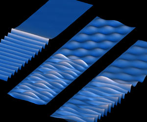
We consider the problem of a horizontal circular cylinder submerged in an infinitely long rectangular channel covered by an ice sheet. A sketch of the problem is shown in figure 1. The channel has half-width  $b$ and calm water depth
  $H$. The density and thickness of the homogeneous ice sheet are assumed to be constant and represented by
  $\rho _i$ and
  $h_i$, respectively, and the density of the water is
  $\rho$. A Cartesian coordinate system
  $O$-
$O$- $xyz$ is defined with the origin located on the central line of the water surface, the
  $x$-axis along the longitudinal direction of the channel and the
  $z$-axis pointing upwards. The centre line of the cylinder is located at
  $x=x_0$ and
  $z=z_0$ and its radius is equal to
  $r_0$.

Figure 1. Sketch of the problem: (a) three-dimensional view; (b) a cross-section view of the channel in the negative  $x$-direction.
It is assumed that the fluid is ideal, incompressible, its motion is irrotational and the linearized velocity potential theory is employed. As discussed in the introduction, due to the ice sheet and its edge conditions, the problem will be three-dimensional. The total velocity potential is written as
 \begin{equation} \varPhi ={-}Ux + \phi, \end{equation}
where  $U$ denotes the speed of the uniform current from
  $x=+\infty$,
  $\phi (x,y,z,t)$ is the disturbed velocity potential by the cylinder, which satisfies the Laplace equation in the entire fluid domain,
 \begin{equation} \nabla^2\phi = \frac{\partial^2 \phi}{\partial x^2} + \frac{\partial^2 \phi}{\partial y^2} + \frac{\partial^2 \phi}{\partial z^2},\quad -\infty< x<{+}\infty,\enspace -b\leq y\leq b,\enspace -H\leq z \leq 0. \end{equation}
The deflection of the ice plate  $\eta (x,y,t)$ should satisfy the Euler–Bernoulli equation on
  $z=0$,
 \begin{equation} \rho_i h_i\eta_{tt} + L\nabla^4\eta = p,\quad z=0, \end{equation}
where  $L=Eh_i^3/[12(1-\nu ^2)]$ denotes the flexural rigidity of the ice sheet,
  $E$ and
  $\nu$ represent its Young's modulus and Poisson ratio, respectively. The fluid pressure
  $p$ on the right-hand side of (2.3) is the excessive fluid pressure and does not include the weight of ice. It can be calculated through the linearized Bernoulli equation
 \begin{equation} p={-}\rho\left(\frac{\partial \phi}{\partial t}-U\frac{\partial \phi}{\partial x}+g\eta\right),\quad z=0, \end{equation}
where  $g$ is the acceleration due to gravity. The kinematic boundary condition can be written as
 \begin{equation} \left(\frac{\partial }{\partial t}-U\frac{\partial}{\partial x}\right)\eta = \frac{\partial \phi}{\partial z},\quad z=0. \end{equation}
For steady flow,  $\partial /\partial t=0$. We have
 $$\begin{gather} \left(L\nabla^4+\rho g\right)\eta=\rho U\frac{\partial \phi}{\partial x},\quad z=0, \end{gather}$$
 $$\begin{gather}-U\frac{\partial \eta}{\partial x}=\frac{\partial \phi}{\partial z},\quad z=0, \end{gather}$$
in which (2.6) is obtained by substituting (2.4) into (2.3). The impermeable condition on the cylinder surface  $S_B$ can be written as
 \begin{equation} \frac{\partial \phi}{\partial n}=Un_x,\quad \text{on}\ S_B, \end{equation}
where  $\boldsymbol {n}=(n_x,0,n_z)$ is the unit normal vector of
  $S_B$, which is pointing out of the fluid domain. Similarly, the impermeable boundary conditions on the rigid sidewalls and bottom of the channel can be expressed as
 $$\begin{gather} \frac{\partial \phi}{\partial y}=0,\quad y={\pm} b, \end{gather}$$
 $$\begin{gather}\frac{\partial \phi}{\partial z}=0,\quad z={-}H. \end{gather}$$
Different from free surface problems, there are also edge conditions at intersection lines of the ice sheet with the two sidewalls, or  $y=\pm b$,
  $z=0$, which can be written as (Timoshenko & Woinowsky-Krieger Reference Timoshenko and Woinowsky-Krieger1959)
 \begin{equation} \left.\begin{gathered} \eta = 0,\quad \frac{\partial \eta}{\partial y}=0,\quad \text{clamped edge,}\\ \eta = 0,\quad \frac{\partial^2\eta}{\partial y^2} + \nu \frac{\partial^2\eta}{\partial x^2}=0,\quad \text{simply supported edge,}\\ \frac{\partial^2\eta}{\partial y^2} + \nu\frac{\partial^2\eta}{\partial x^2}=0,\quad \frac{\partial^3\eta}{\partial y^3}+(2-\nu) \frac{\partial^3\eta}{\partial x^2\partial y}=0,\quad \text{free edge,} \end{gathered}\right\}. \end{equation}
The radiation condition at far-field  $x\to \pm \infty$ can be written as
 \begin{equation} \frac{\partial \phi}{\partial x}=\mathcal{U}_{{\pm}}(x,y,z),\quad x\to\pm\infty, \end{equation}
where  $\mathcal {U}_\pm (x,y,z)$ represents waves generated by the cylinder. The waves can have multiple components and the group velocities of the waves at
  $x\to +\infty$ and
  $x\to -\infty$ are larger and smaller than
  $U$, respectively. This will be discussed in detail later.
3. Solution procedures
3.1. The Green function: velocity potential due to a single source
The Green function  $G(x,y,z,x_0,y_0,z_0)$ is the velocity potential at point
  $P(x,y,z)$ due to a source at
  $P_0(x_0,y_0,z_0)$, which satisfies the following equation:
 \begin{equation} \nabla^2G=\delta(x-x_0)\delta(y-y_0)\delta(z-z_0), \end{equation}
where  $\delta (x)$ is the Dirac delta function. Here
  $\xi (x,y,x_0,y_0,z_0)$ is defined as the wave elevation at point
  $(x,y)$ induced by the source at
  $P_0(x_0,y_0,z_0)$. Furthermore,
  $G(x,y,z,x_0,y_0,z_0)$ and
  $\xi (x,y,x_0,y_0,z_0)$ also need to satisfy the boundary conditions (2.6), (2.7) and (2.9)–(2.12).
Performing the Fourier transform for  $G$ and
  $\xi$ in the
  $x$-direction
 \begin{equation} \left.\begin{gathered} \hat{G}=\int_{-\infty}^{+\infty}G\,\text{e}^{-\text{i}kx}\,{\text{d}\kern0.7pt x}\\ \hat{\xi}=\int_{-\infty}^{+\infty}\xi \,\text{e}^{-\text{i}kx}\,{\text{d}\kern0.7pt x} \end{gathered}\right\}, \end{equation}
and applying (3.2) to (3.1), we have
 \begin{equation} -k^2\hat{G}+\frac{\partial^2\hat{G}}{\partial y^2}+ \frac{\partial^2\hat{G}}{\partial z^2}=\delta(y-y_0)\delta(z-z_0)\,\text{e}^{-\text{i}kx_0}. \end{equation}
Based on the impermeable condition in (2.9),  $\hat {G}$ can be further expanded into an orthogonal series of cosine functions in the
  $y$-direction. Using the condition in (2.10), the solution of (3.3) can be written in the following form:
 \begin{equation} \hat{G}=\sum_{n=0}^{+\infty}Z_n(k,z,x_0,y_0,z_0)\cos\sigma_n(y+b), \end{equation}
where
 \begin{align} & Z_n(k,z,x_0,y_0,z_0) \nonumber\\ &\quad ={-}\frac{[\exp({-K_n|z-z_0|})+\exp({-K_n(z+z_0+2H)})]\, \text{e}^{-\text{i}kx_0}\cos\sigma_n(y_0+b)}{2(1+\delta_{n0})bK_n} \nonumber\\ &\qquad +b_n\frac{\text{e}^{-\text{i}kx_0}\cosh K_n(z+H)}{\cosh K_nH}, \end{align}
 $\sigma _n=n{\rm \pi} /2b$,
  $K_n=\sqrt {k^2+\sigma _n^2}$ and where
  $\delta _{ij}$ denotes the Kronecker delta function. The terms of
  $b_n$ in (3.5) correspond to the general solution of (3.3) when the right-hand side is zero. Here
  $b_n$ are to be determined by the conditions on the ice sheet. Applying the Fourier transform to (2.6) and (2.7), we have
 $$\begin{gather} (\rho g + Lk^4)\hat{\xi}-2Lk^2\frac{\partial^2 \hat{\xi}}{\partial y^2}+L \frac{\partial^4 \hat{\xi}}{\partial y^4}=\text{i}k\rho U\hat{G}, \end{gather}$$
 $$\begin{gather}-\text{i}kU\hat{\xi}=\frac{\partial \hat{G}}{\partial z}. \end{gather}$$
We choose to follow the approach taken by Ren et al. (Reference Ren, Wu and Li2020), which involves expanding  $\partial ^4\hat {\xi }/\partial y^4$ rather than
  $\hat {\xi }$ into a cosine series, thus
 \begin{equation} \frac{\partial^4\hat{\xi}}{\partial y^4}=\text{e}^{-\text{i}kx_0}\sum_{n=0}^{+\infty}a_n\cos\sigma_n(y+b). \end{equation}
Then, through integration four times,  $\hat {\xi }$ can be obtained as
 \begin{equation} \hat{\xi}=\text{e}^{-\text{i}kx_0}\left[c_0+c_1y+c_2y^2+c_3y^3+ \frac{a_0}{24}y^4+\sum_{n=1}^{+\infty}\frac{a_n}{\sigma_n^4}\cos\sigma_n(y+b)\right], \end{equation}
where  $a_n\ (n=0,1,2\cdots )$ are unknown coefficients and are functions of
  $k$,
$k$,  $c_i\ (i=0\sim 3)$ are four constants which can be linked to
  $a_n$ through edge conditions. It should be mentioned here that
  $c_0$,
  $c_2$ and
  $a_{2n}$ correspond to symmetric components, while
  $c_1$,
  $c_3$ and
  $a_{2n+1}$ correspond to antisymmetric components. Substituting (3.4), (3.5) and (3.9) into (3.6) and (3.7), we have
 \begin{align} & (\rho g+Lk^4)\left[c_0+c_1y+c_2y^2+c_3y^3+\frac{a_0}{24}y^4+ \sum_{n=1}^{+\infty}\frac{a_n}{\sigma_n^4}\cos\sigma_n(y+b)\right] \nonumber\\ &\qquad -2k^2L\left[2c_2+6c_3y+\frac{a_0}{2}y^2-\sum_{n=1}^{+\infty} \frac{a_n}{\sigma_n^2}\cos\sigma_n(y+b)\right]+L\sum_{n=0}^{+\infty}a_n\cos\sigma_n(y+b) \nonumber\\ &\quad =\text{i}k\rho U\sum_{n=0}^{+\infty}\left[-\frac{\text{e}^{{-}K_nH}\cosh K_n(z_0+H)}{(1+\delta_{n0})bK_n}\cos \sigma_n(y_0+b)+b_n\right]\cos\sigma_n(y+b), \end{align}
 \begin{align} & -\text{i}kU\left[c_0+c_1y+c_2y^2+c_3y^3+\frac{a_0}{24}y^4+ \sum_{n=1}^{+\infty}\frac{a_n}{\sigma_n^4}\cos\sigma_n(y+b)\right] \nonumber\\ &\quad =\sum_{n=0}^{+\infty}\left[\frac{\text{e}^{{-}K_nH}\cosh K_n(z_0+H)}{(1+\delta_{n0})b} \cos\sigma_n(y_0+b)+b_nK_n\tanh K_nH\right]\cos\sigma_n(y+b). \end{align}
The term  $y^j\ (\kern0.06em j=0\sim 4)$ can be further expanded into the orthogonal series of cosine functions as
 \begin{equation} y^j=\sum_{n=0}^{+\infty}d_n^{(\kern0.06em j)}\cos\sigma_n(y+b). \end{equation}
Then, (3.10) and (3.11) can be written as
 \begin{align} & (\rho g+Lk^4)\left[c_0d_n^{(0)}+c_1d_n^{(1)}+c_2d_n^{(2)}+c_3d_n^{(3)}+ \frac{a_0}{24}d_n^{(4)}+\frac{(1-\delta_{n0})a_n}{\sigma_n^4}\right] \nonumber\\ &\qquad -2k^2L\left[2c_2d_n^{(0)}+6c_3d_n^{(1)}+\frac{a_0}{2}d_n^{(2)}- \frac{(1-\delta_{n0})a_n}{\sigma_n^2}\right]+La_n \nonumber\\ &\quad =\text{i}k\rho U\left[-\frac{\text{e}^{{-}K_nH}\cosh K_n(z_0+H)}{(1+\delta_{n0})bK_n} \cos\sigma_n(y_0+b)+b_n\right],\quad n=0,1,2\cdots \end{align}
 \begin{align} & -\text{i}kU\left[c_0d_n^{(0)}+c_1d_n^{(1)}+c_2d_n^{(2)}+c_3d_n^{(3)}+ \frac{a_0}{24}d_n^{(4)}+\frac{(1-\delta_{n0})a_n}{\sigma_n^4}\right] \nonumber\\ &\quad =\left[\frac{\text{e}^{{-}K_nH}\cosh K_n(z_0+H)}{(1+\delta_{n0})b}\cos \sigma_n(y_0+b)+b_nK_n\tanh K_nH\right],\quad n=0,1,2\cdots . \end{align}
From (3.13) and (3.14),  $a_n$ and
  $b_n$ can be expressed as
 $$\begin{gather} a_n = \alpha_{n,0}c_0+\alpha_{n,1}c_1+\alpha_{n,2}c_2+ \alpha_{n,3}c_3+\text{i}R_n,\quad n=0,1,2\cdots \end{gather}$$
 $$\begin{gather}b_n = \frac{1}{K_n\tanh K_nH}\left(\text{i}\beta_{n,0}c_0+\text{i}\beta_{n,1}c_1+\text{i}\beta_{n,2}c_2+\text{i}\beta_{n,3}c_3+S_n\right),\quad n=0,1,2\cdots \end{gather}$$
where
 \begin{align} \alpha_{n,j} &= \frac{1}{\varDelta_n}\left\{\begin{aligned} & d_n^{(\kern0.06em j)}\left[(\rho g+Lk^4)K_n\tanh K_nH -\rho k^2U^2\right]\\ & -4\delta_{2j}k^2Ld_n^{(0)}K_n\tanh K_nH-12\delta_{3j}k^2Ld_n^{(1)}K_n\tanh K_nH \end{aligned}\right\} \nonumber\\ &\quad +(1-\delta_{n0})\gamma_n\alpha_{0,j}, \end{align}
 \begin{equation} \beta_{n,j}={-}Uk\left[d_n^{(\kern0.06em j)}+\frac{d_n^{(4)}}{24}\alpha_{0,j}+ \frac{(1-\delta_{n0})}{\sigma_n^4}\alpha_{n,j}\right],\quad j=0\sim3 \end{equation}
and
 $$\begin{gather} R_n=\frac{\rho Uk\cosh K_n(z_0+H)\cos\sigma_n(y_0+b)}{(1+\delta_{n0})b \varDelta_n\cosh K_nH}+(1-\delta_{n0})\gamma_nR_0, \end{gather}$$
 $$\begin{gather}S_n=kU\left(\frac{d_n^{(4)}}{24}R_0+\frac{1-\delta_{n0}}{\sigma_n^4}R_n\right)-\frac{\text{e}^{{-}K_nH}\cosh K_n(z_0+H)\cos\sigma_n(y_0+b)}{(1+\delta_{n0})b}, \end{gather}$$
with
 $$\begin{gather} \varDelta_n=\left\{\begin{aligned} & \delta_{n0}\left[-\left(\frac{\rho g+Lk^4}{24}d_n^{(4)}-k^2Ld_n^{(2)}+L\right)K_n\tanh K_nH+ \frac{\rho k^2U^2d_n^{(4)}}{24}\right]\\ & \quad +(1-\delta_{n0})\left[-\left(\frac{\rho g+Lk^4}{\sigma_n^4}+ \frac{2k^2L}{\sigma_n^2}+L\right)K_n\tanh K_nH+\frac{\rho k^2U^2}{\sigma_n^4}\right] \end{aligned}\right\}, \end{gather}$$
 $$\begin{gather}\gamma_n=\frac{1}{\varDelta_n}\left[\left(\frac{\rho g+Lk^4}{24}d_n^{(4)}-k^2Ld_n^{(2)}\right)K_n \tanh K_nH-\frac{\rho k^2U^2d_n^{(4)}}{24}\right]. \end{gather}$$
If we consider the symmetric or antisymmetric nature of  $y^j$
$y^j$  $(\kern0.06em j=0\sim 3)$, we will have
  $d_{2n}^{(2j+1)}=d_{2n+1}^{(2j)}=0$
  $(\kern0.06em j=0, 1)$. This leads to
  $\gamma _{2n+1}=0$ and
  $\alpha _{2n+1,2j}=\alpha _{2n,2j+1}=0$
  $(\kern0.06em j=0, 1,\ n\geq 0)$. As a result,
  $a_n$ can be further expressed as
 \begin{equation} \left.\begin{gathered} a_{2n}=\alpha_{2n,0}c_0+\alpha_{2n,2}c_2+\text{i}R_{2n}\\ a_{2n+1}=\alpha_{2n+1,1}c_1+\alpha_{2n+1,3}c_3+\text{i}R_{2n+1} \end{gathered}\right\}. \end{equation}
It can be seen from (3.20) that  $a_{2n}$ depend on two unknown coefficients
  $c_0$ and
  $c_2$, while
  $a_{2n+1}$ depend on
  $c_1$ and
  $c_3$;
  $b_n$ can be also treated in a similar way. The four unknown coefficients
  $c_i$
$c_i$  $(i=0\sim 3)$ can be determined from the four edge conditions, including those in (2.11). As a result, a system of linear equations of the following form can be established:
 \begin{equation} [\boldsymbol{\mathcal{A}}][\boldsymbol{C}]=[\boldsymbol{\mathcal{B}}], \end{equation}
where  $[\boldsymbol {\mathcal {A}}]$ is a
  $4\times 4$ coefficient matrix,
  $[\boldsymbol {C}]$ is a column containing
  $c_i$, and
  $[\boldsymbol {\mathcal {B}}]$ is a known column. For a specific case, this
  $4\times 4$ matrix equation may be further simplified. If the edge conditions at
  $y=\pm b$ are same, (3.21) may be split into two independent
  $2\times 2$ submatrix equations, one for
  $c_0$ and
  $c_2$, and the other for
  $c_1$ and
  $c_3$. As a result, the symmetric and antisymmetric transverse waves in (3.9) become independent to each other. In general,
  $c_i$
$c_i$  $(i=0\sim 3)$ are fully coupled to each other, which leads
  $a_{2n}$ and
  $a_{2n+1}$ in (3.20) to become coupled. The solution of
  $c_i$ can be written as
 \begin{equation} c_i ={-}\text{i}\sum_{m=0}^{+\infty}\frac{\rho Uk\cosh K_m(z_0+H)\cos \sigma_m(y_0+b)}{(1+\delta_{m0})b|\boldsymbol{\mathcal{A}}|\varDelta_m\cosh K_mH}c_{m,i}^{\prime},\quad i=0\sim3, \end{equation}
where  $|\boldsymbol {\mathcal {A}}|$ is the determinant of
  $[\boldsymbol {\mathcal {A}}]$. The elements of
  $[\boldsymbol {\mathcal {A}}]$ and
  $[\boldsymbol {\mathcal {B}}]$, as well as coefficient
  $c_{m,i}^\prime$ are related to edge conditions, an example of these under clamped–clamped edges are given in Appendix A.
Once  $c_i$
$c_i$  $(i=0\sim 3)$,
  $a_n$ and
  $b_n$
$b_n$  $(n=0,1,2\cdots )$ are obtained, then
  $G$ and
  $\xi$ can be obtained through the inverse Fourier transform. Using (Linton & McIver Reference Linton and McIver2001)
 \begin{align} &
\int_{-\infty}^{+\infty}\frac{\delta_{n0}\exp(-K_nH)-\exp({-K_n|z-z_0|+\text{i}k(x-x_0)})}{2K_n}\text{d}
k \nonumber\\ &\quad =\delta_{n0}\ln
\left(\frac{r}{H}\right)-(1-\delta_{n0})\mathscr{K}_0(\sigma_nr),
\end{align}
\begin{align} &
\int_{-\infty}^{+\infty}\frac{\delta_{n0}\exp(-K_nH)-\exp({-K_n|z-z_0|+\text{i}k(x-x_0)})}{2K_n}\text{d}
k \nonumber\\ &\quad =\delta_{n0}\ln
\left(\frac{r}{H}\right)-(1-\delta_{n0})\mathscr{K}_0(\sigma_nr),
\end{align}
 \begin{align} &
\int_{-\infty}^{+\infty}\frac{\delta_{n0}\exp(-K_nH)-\exp({-K_n(z+z_0+2H)+\text{i}k(x-x_0)})}{2K_n}\text{d}
k \nonumber\\ &\quad =\delta_{n0}\ln
\left(\frac{r^{\prime}}{H}\right)-(1-\delta_{n0})\mathscr{K}_0(\sigma_nr^\prime),
\end{align}
\begin{align} &
\int_{-\infty}^{+\infty}\frac{\delta_{n0}\exp(-K_nH)-\exp({-K_n(z+z_0+2H)+\text{i}k(x-x_0)})}{2K_n}\text{d}
k \nonumber\\ &\quad =\delta_{n0}\ln
\left(\frac{r^{\prime}}{H}\right)-(1-\delta_{n0})\mathscr{K}_0(\sigma_nr^\prime),
\end{align}
where  $r=\sqrt {(x-x_0)^2+(z-z_0)^2}$ and
  $r^{\prime }=\sqrt {(x-x_0)^2+(z+z_0+2H)^2}$,
  $\mathscr {K}_n$ denotes the
  $n$th-order modified Bessel function of second kind. We have the Green function
 $$\begin{gather} G(x,y,z,x_0,y_0,z_0)=\sum_{n=0}^{+\infty}\mathcal{Z}_n(x,z,x_0,y_0,z_0)\cos\sigma_n(y+b), \end{gather}$$
 $$\begin{gather}\mathcal{Z}_n(x,z,x_0,y_0,z_0)=\mathcal{Z}_{n,1}+\mathcal{Z}_{n,2}, \end{gather}$$
and
 \begin{align} \mathcal{Z}_{n,1} &=
\frac{1}{4{\rm \pi} b}\left\{\delta_{n0}\left[\ln
\left(\frac{r}{H}\right)+\ln\left(\frac{r^{\prime}}{H}\right)\right]-2(1-\delta_{n0})
\left[\mathscr{K}_0(\sigma_nr)+ \mathscr{K}_0(\sigma_n
r^{\prime})\right]\right\} \nonumber\\ &\quad
\times\cos\sigma_n(y_0+b),
\end{align}
\begin{align} \mathcal{Z}_{n,1} &=
\frac{1}{4{\rm \pi} b}\left\{\delta_{n0}\left[\ln
\left(\frac{r}{H}\right)+\ln\left(\frac{r^{\prime}}{H}\right)\right]-2(1-\delta_{n0})
\left[\mathscr{K}_0(\sigma_nr)+ \mathscr{K}_0(\sigma_n
r^{\prime})\right]\right\} \nonumber\\ &\quad
\times\cos\sigma_n(y_0+b),
\end{align}
 \begin{align} \mathcal{Z}_{n,2}&
=\frac{\rho U}{2{\rm \pi}
b}\int_{\mathscr{L}}\sum_{m=0}^{+\infty}\frac{\begin{array}{l}\left\{ k\mu_{n,m}\cosh
K_m(z_0+H) \cos\sigma_m(y_0+b)\right.\\\left. \quad \times\left[\cosh
K_n(z+H)\exp({\text{i}k(x-x_0)})-
\delta_{n0}\right]\right\}\end{array}}{(1+\delta_{m0})|\boldsymbol{\mathcal{A}}|\varDelta_mK_n\sinh
K_nH\cosh K_mH}\text{d} k,
\end{align}
\begin{align} \mathcal{Z}_{n,2}&
=\frac{\rho U}{2{\rm \pi}
b}\int_{\mathscr{L}}\sum_{m=0}^{+\infty}\frac{\begin{array}{l}\left\{ k\mu_{n,m}\cosh
K_m(z_0+H) \cos\sigma_m(y_0+b)\right.\\\left. \quad \times\left[\cosh
K_n(z+H)\exp({\text{i}k(x-x_0)})-
\delta_{n0}\right]\right\}\end{array}}{(1+\delta_{m0})|\boldsymbol{\mathcal{A}}|\varDelta_mK_n\sinh
K_nH\cosh K_mH}\text{d} k,
\end{align}
where
 \begin{align} \mu_{n,m} &= \sum_{j=0}^{3}\beta_{n,j}c_{m,j}^{\prime}+\delta_{m0}|\boldsymbol{\mathcal{A}}|Uk \left(\frac{d_n^{(4)}}{24}+\frac{(1-\delta_{n0})\gamma_n}{\sigma_n^4}\right) \nonumber\\ &\quad +\delta_{nm}|\boldsymbol{\mathcal{A}}|\left[\frac{Uk(1-\delta_{n0})}{\sigma_n^4}- \frac{\varDelta_n(1+\text{e}^{{-}2K_nH})}{2\rho Uk}\right]. \end{align}
 It should be mentioned that a constant term is, respectively, added to  $\mathcal {Z}_{n,1}$ and
  $\mathcal {Z}_{n,2}$ in (3.26) to remove the high-order singularity at
  $k=0$, which will not affect the results as all the equations for
  $G$ involve only its spatial derivatives. The term
  $\mathcal {Z}_{n,1}$ is obtained based on the derivation in Li, Wu & Ren (Reference Li, Wu and Ren2021). There will be singularities in
  $\mathcal {Z}_{n,2}$ when
  $|\boldsymbol {\mathcal {A}}|(k)=0$. Because
  $|\boldsymbol {\mathcal {A}}|(k)$ is an even function, all its real roots can be represented by
  $\pm k_s$
  $(s=1\cdots S)$, with
  $k_s>0$. In the case of Ren et al. (Reference Ren, Wu and Li2020) for wave propagation in the channel, each
  $k_s$ corresponds to the dispersion relationship between the wave frequency and wavenumber. Here, mathematically, each
  $k_s$ corresponds to a singularity in the integrand of the inverse Fourier transform. Physically, it corresponds to each wave generated by the source in the channel. The number of singularities can be more than one, and the value of
  $S$ depends on the current speed
  $U$ when other parameters are fixed, which will be discussed in detail later. The way to treat each singularity will depend on the group velocity of its corresponding wave. The wave will be at upstream
  $(x=+\infty )$ or downstream
  $(x=-\infty )$ if its group velocity is larger or smaller than
  $U$, respectively. Based on this, the integration route
  $\mathscr {L}$ in
  $\mathcal {Z}_{n,2}$ from
  $-\infty$ to
  $+\infty$ can be defined as follows. We may consider the integration of
  $f(k)\,\text {e}^{\text {i}kx}/(k-k_s)$ along the path
  $\mathscr {L}$. This can be split into the principle integration and a contribution from the pole. If the group velocity of the wave component
  $k_s$ is larger (smaller) than
  $U$,
$U$,  $\mathscr {L}$ passes over (under) the singularities at
  ${\pm }k_s$. Thus, the contribution from the pole at
  $k=k_s$ will be
  $-\text {i}{\rm \pi} f(k_s)\,\text {e}^{\text {i}k_sx}$ or
  $+\text {i}{\rm \pi} f(k_s)\,\text {e}^{\text {i}k_sx}$. If we use (Wehausen & Laitone Reference Wehausen and Laitone1960)
 \begin{equation} \lim_{|x|\to+\infty}\text{P.V.}\int_{-\infty}^{+\infty} \frac{f(k)}{k-k_s}\text{e}^{\text{i}kx}\,\text{d} k=\text{sgn}(x)\text{i}{\rm \pi} f(k_s)\,\text{e}^{\text{i}k_sx}, \end{equation}
in the integral in  $\mathcal {Z}_{n,2}$, we can find that the radiation condition (2.12) is satisfied.
It may be of interest to see that the Green function is symmetric about the source and field points, or  $G(x,y,z,x_0,y_0,z_0)=G(x_0,y_0,z_0,x,y,z)$, which is shown in Appendix B.
3.2. Multipole expansion for the horizontal circular cylinder
The Green function derived above can be used to convert the governing equation to an integral equation over the surface of a body with arbitrary shape. For some special geometries, such as a sphere, the solution may be found through expansion in terms of the multipole obtained through differentiating the Green function with respect to the position of the source (see, for example, Wu (Reference Wu1998b)). For a horizontal circular cylinder, the potential can be expanded into the cosine series as used for  $G$. The governing Laplace equation in
  $(x,y,z)$ then becomes the modified Helmholtz equation in
  $(x,z)$ for a circular section. Subsequently, the solution of the modified Helmholtz equation can be obtained from a two-dimensional multipole expansion. To construct that, we may apply a source distribution
  $\varsigma (y_0)$ along the centre line of the cylinder. This is then expanded into the cosine series, or
  $\varsigma (y_0)=\sum _{n=0}^{+\infty }\mathcal {V}_n\cos \sigma _n(y_0+b)$. It will create the following potential:
 \begin{equation} \varphi=\sum_{n=0}^{+\infty}{\mathcal{V}_n\int_{{-}b}^{b}G\cos{\sigma_n(y_0+b)}\,\text{d} y_0}, \end{equation}
where  $G$ is the Green function derived in the previous section. Substituting (3.24) into (3.29), we obtain
 \begin{equation} \varphi=\sum_{n=0}^{+\infty}{\varphi_n\cos{\sigma_n\left(y+b\right)}}, \end{equation}
where
 \begin{equation} \varphi_n=\varphi_{n,1}+\varphi_{n,2}, \end{equation}
with
 \begin{align} \varphi_{n,1}&=\frac{\mathcal{V}_n}{2{\rm \pi}}\left\{\delta_{n0} \left[\ln \left(\frac{r}{H}\right)+\ln\left(\frac{r^{\prime}}{H}\right)\right]-(1-\delta_{n0}) \left[\mathscr{K}_0(\sigma_n r)+\mathscr{K}_0(\sigma_n r^{\prime})\right]\right\}, \end{align}
 \begin{align} \varphi_{n,2}&=\frac{\rho U}{2{\rm \pi}} \nonumber\\ &\quad \times\int_{\mathscr{L}}\sum_{n^\prime=0}^{+\infty}\frac{\mathcal{V}_{n^\prime} \mu_{n,n^\prime}k\cosh K_{n^\prime}(z_0+H)\left[\cosh K_n(z+H)\exp({\text{i}k(x-x_0)})-\delta_{n0}\right]}{|\boldsymbol{\mathcal{A}}|\varDelta_{n^\prime}K_n \sinh K_nH \cosh K_{n^\prime}H}\text{d} k. \end{align}
We may use the operator
 \begin{equation} \left(D_{{\pm}}\right)^m={-}\frac{1}{2^{m-1}\left(m-1\right)!} \left(\frac{\partial}{\partial z_0}\pm \text{i}\frac{\partial}{\partial x_0}\right)^m. \end{equation}
This gives (Linton & McIver Reference Linton and McIver2001)
 $$\begin{gather} \left(D_{{\pm}}\right)^m\ln{r}=\frac{\text{e}^{{\pm} \text{i}m\theta}}{r^m}, \end{gather}$$
 $$\begin{gather}\left(D_{{\pm}}\right)^m\mathscr{K}_0\left(\sigma_nr\right)= \frac{\left({-}1\right)^m\sigma_n^m}{2^{m-1}\left(m-1\right)!}\text{e}^{{\pm} \text{i}m\theta}\mathscr{K}_m\left(\sigma_nr\right), \end{gather}$$
where  $z-z_0=r\cos {\theta }$ and
  $x-x_0=r\sin {\theta }$. As mentioned in Li, Wu & Shi (Reference Li, Wu and Shi2019), because
  $\varphi$ is a real function, we may apply only the operator
  $(D_+)^m$. Using
 $$\begin{gather} \left(D_+\right)^m\exp({\pm K_nz_0\pm \text{i}kx_0})={-}\frac{({\pm} 1)^m(K_n-k)^m}{2^{m-1}(m-1)!}\exp({\pm K_nz_0\pm \text{i}kx_0}), \end{gather}$$
 $$\begin{gather}\left(D_+\right)^m\exp({\pm K_nz_0\mp \text{i}kx_0})={-}\frac{({\pm} 1)^m(K_n+k)^m}{2^{m-1}(m-1)!}\exp({\pm K_nz_0\mp \text{i}kx_0}), \end{gather}$$
as well as (3.34), the velocity potential of the multipole can be expressed as
 $$\begin{gather} \left(\varphi_+\right)^m=\left(D_{+}\right)^m\varphi= \sum_{n=0}^{+\infty}\left(\varphi_+\right)_n^m\cos{\sigma_n(y+b)}, \end{gather}$$
 $$\begin{gather}\left(\varphi_+\right)_n^m=\left(\varphi_+\right)_{n,1}^m+\left(\varphi_+\right)_{n,2}^m+ \left(\varphi_+\right)_{n,3}^m, \end{gather}$$
where  $(\varphi _+)_{n,1}^m+(\varphi _+)_{n,2}^m=(D_{+})^m\varphi _{n,1}$,
  $(\varphi _+)_{n,3}^m=(D_{+})^m\varphi _{n,2}$ and can be obtained as
 $$\begin{gather} \left(\varphi_+\right)_{n,1}^m=\frac{\mathcal{V}_n}{2{\rm \pi}} \left[\delta_{n0}\frac{\text{e}^{\text{i}m\theta}}{r^m}-(1-\delta_{n0}) \frac{({-}1)^m\sigma_n^m}{2^{m-1}(m-1)!}\text{e}^{\text{i}m\theta}\mathscr{K}_m(\sigma_nr)\right], \end{gather}$$
 $$\begin{gather}\left(\varphi_+\right)_{n,2}^m=\frac{({-}1)^m\mathcal{V}_n}{2^{m+1}(m-1)!{\rm \pi}} \int_{-\infty}^{+\infty}\frac{(K_n-k)^m\exp({-K_n(z+z_0+2H)+\text{i}k(x-x_0)})}{K_n}\text{d} k, \end{gather}$$
 \begin{gather} \hspace{-21pc}(\varphi_+)_{n,3}^{m} = \frac{-\rho U}{2^{m+1}(m-1)!{\rm \pi}} \nonumber\\ \hspace{3.5pc}\times\int_{\mathscr{L}}\sum_{n^\prime=0}^{+\infty} \frac{\mathcal{V}_{n^\prime}\mu_{n,n^\prime}k\cosh K_n(z+H)E_{n^{\prime},m}(k,z_0)\exp({\text{i}k(x-x_0)})}{|\boldsymbol{\mathcal{A}}|\varDelta_{n^\prime}K_n \sinh K_nH \cosh K_{n^{\prime}}H}\text{d} k, \end{gather}
with
 \begin{align} E_{n^{\prime},m}(k,z_0)=(K_{n^{\prime}}+k)^m\exp({K_{n^{\prime}}(z_0+H)})+ ({-}1)^m(K_{n^{\prime}}-k)^m\exp({-K_{n^{\prime}}(z_0+H)}). \end{align}
The potential  $\phi$ due to the cylinder then can be written in a multipole expansion form as
 \begin{equation} \phi=\text{Re}\left\{\sum_{m=1}^{+\infty}{r_0^mg_m(\varphi_+)^m}\right\}. \end{equation}
It then satisfies all the boundary conditions met by the Green function and the only remaining one is that on the cylinder surface. To satisfy the body surface boundary condition, we may write the potential in the polar coordinate system. Using (Abramowitz & Stegun Reference Abramowitz and Stegun1970)
 \begin{equation} \left.\begin{gathered} \exp({K_n(z-z_0)\pm \text{i}k(x-x_0)})=\sum_{m=0}^{+\infty}T_{n,m}(r) \left[A_{n,m}^\pm(k)\,\text{e}^{\text{i}m\theta}+A_{n,m}^\mp(k)\,\text{e}^{-\text{i}m\theta}\right]\\ \exp({-K_n(z-z_0)\pm \text{i}k(x-x_0)})=\sum_{m=0}^{+\infty}({-}1)^mT_{n,m}(r) \left[A_{n,m}^\mp(k)\,\text{e}^{\text{i}m\theta}+A_{n,m}^\pm(k)\,\text{e}^{-\text{i}m\theta}\right] \end{gathered}\right\}, \end{equation}
where
 \begin{equation} \left.\begin{gathered} A_{n,m}^+(k)=\delta_{n0}k^m+\left(1-\delta_{n0}\right)\left(\frac{K_n+k}{\sigma_n}\right)^m\\ A_{n,m}^-(k)=\left(1-\delta_{n0}\right)\left(1-\delta_{m0}\right)\left(\frac{\sigma_n}{K_n+k}\right)^m\\ T_{n,m}(r)=\delta_{n0}\frac{r^m}{m!}+\left(1-\delta_{n0}\right)\mathscr{I}_m\left(\sigma_nr\right) \end{gathered}\right\}, \end{equation}
and  $\mathscr {I}_m$ denotes the
  $m$th-order modified Bessel function of first kind, we have
 \begin{equation}
\phi=\text{Re}\left\{\sum_{n=0}^{+\infty}\sum_{m=0}^{+\infty}
\begin{aligned} & \left[\begin{aligned} &
Q_{n,m}f_{n,m}\,\text{e}^{\text{i}m\theta}+T_{n,m}
\sum_{m^\prime=1}^{+\infty}f_{n,m^\prime}\left(\mathcal{C}_{n,m,m^\prime}^+
\text{e}^{\text{i}m\theta}+\mathcal{C}_{n,m,m^\prime}^-\text{e}^{-\text{i}m\theta}\right)\\
& \quad
+T_{n,m}\sum_{n^\prime=0}^{+\infty}\sum_{m^\prime=1}^{+\infty}f_{n^\prime,m^\prime}
\left(\mathcal{D}_{n,n^\prime,m,m^\prime}^+\text{e}^{\text{i}m\theta}+
\mathcal{D}_{n,n^\prime,m,m^\prime}^-\text{e}^{-\text{i}m\theta}\right)
\end{aligned}\right]\\ &\times\cos{\sigma_n(y+b)}
\end{aligned}\right\}, \end{equation}
\begin{equation}
\phi=\text{Re}\left\{\sum_{n=0}^{+\infty}\sum_{m=0}^{+\infty}
\begin{aligned} & \left[\begin{aligned} &
Q_{n,m}f_{n,m}\,\text{e}^{\text{i}m\theta}+T_{n,m}
\sum_{m^\prime=1}^{+\infty}f_{n,m^\prime}\left(\mathcal{C}_{n,m,m^\prime}^+
\text{e}^{\text{i}m\theta}+\mathcal{C}_{n,m,m^\prime}^-\text{e}^{-\text{i}m\theta}\right)\\
& \quad
+T_{n,m}\sum_{n^\prime=0}^{+\infty}\sum_{m^\prime=1}^{+\infty}f_{n^\prime,m^\prime}
\left(\mathcal{D}_{n,n^\prime,m,m^\prime}^+\text{e}^{\text{i}m\theta}+
\mathcal{D}_{n,n^\prime,m,m^\prime}^-\text{e}^{-\text{i}m\theta}\right)
\end{aligned}\right]\\ &\times\cos{\sigma_n(y+b)}
\end{aligned}\right\}, \end{equation}
where
 $$\begin{gather} Q_{n,m}(r)=\frac{(1-\delta_{m0})}{2{\rm \pi}}\left[\delta_{n0}\left(\frac{r_0}{r}\right)^m- \frac{(1-\delta_{n0})(-\sigma_nr_0)^m}{2^{m-1}(m-1)!}\mathscr{K}_m(\sigma_nr)\right], \end{gather}$$
 $$\begin{gather}\mathcal{C}_{n,m,m^{\prime}}^{{\pm}}=\frac{({-}1)^{m+m^{\prime}} r_0^{m^{\prime}}}{2^{m^{\prime}+1}(m^{\prime}-1)!{\rm \pi}}\int_{-\infty}^{+\infty} \frac{(K_n-k)^{m^{\prime}}\exp({-2K_n(z_0+H)})A_{n,m}^{{\mp}}}{K_n}\text{d} k, \end{gather}$$
 \begin{gather} \hspace{-19pc}\mathcal{D}_{n,n^{\prime},m,m^{\prime}}^{{\pm}}=\frac{-\rho Ur_0^{m^{\prime}}}{2^{m^{\prime}+2}(m^{\prime}-1)!{\rm \pi}} \nonumber\\ \hspace{2pc} \times\int_{\mathscr{L}} \frac{\mu_{n,n^\prime}k\left[\exp({K_n(z_0+H)})A_{n,m}^{{\pm}}+({-}1)^m\exp({-K_n(z_0+H)})A_{n,m}^{{\mp}}\right] E_{n^{\prime},m^{\prime}}}{\varDelta_{n^\prime}|\boldsymbol{\mathcal{A}}|K_n \sinh K_nH \cosh K_{n^{\prime}}H}\text{d} k.\nonumber\\ \end{gather}
It should be mentioned here that a new unknown coefficient  $f_{n,m}$ is defined as
  $f_{n,m}=\mathcal {V}_ng_m$. The impermeable condition on the body surface in (2.8) gives
 \begin{align} & Q_{n,m}^\prime(r_0)f_{n,m}+T_{n,m}^\prime(r_0) \sum_{m^\prime=1}^{+\infty}\left(f_{n,m^\prime}\mathcal{C}_{n,m,m^\prime}^+{+}{\bar{f}}_{n,m^\prime}{\bar{\mathcal{C}}}_{n,m,m^\prime}^-\right) \nonumber\\ &\quad +T_{n,m}^\prime(r_0)\sum_{n^\prime=0}^{+\infty}\sum_{m^\prime=1}^{+\infty} \left(f_{n^\prime,m^\prime}\mathcal{D}_{n,n^\prime,n,m^\prime}^+{+}{\bar{f}}_{n^\prime,m^\prime}{\bar{\mathcal{D}}}_{n,n^\prime,m,m^\prime}^-\right)={-}\text{i} \delta_{n0}\delta_{m1}U, \end{align}
where  $n=0,1,2\cdots$ and
  $m=1,2,3\cdots$
  $Q_{n,m}^\prime$ (
 $T_{n,m}^\prime$) represents the derivative of
  $Q_{n,m}$ (
 $T_{n,m}$) with respect to
  $r$, which can be obtained as
 \begin{equation} \left.\begin{gathered} Q_{n,m}^\prime(r)=\frac{(1-\delta_{m0})}{2{\rm \pi}}\left[-\delta_{n0}m\frac{r_0^m}{r^{m+1}}+ \frac{(1-\delta_{n0})(-\sigma_nr_0)^{m+1}}{2^{m-1}(m-1)!r_0}\mathscr{K}_m^\prime(\sigma_nr)\right]\\ T_{n,m}^\prime(r)=\delta_{n0}\frac{r^{m-1}}{(m-1)!}+(1-\delta_{n0})\sigma_n\mathscr{I}_m^\prime(\sigma_nr) \end{gathered}\right\}. \end{equation}
After (3.45) is solved,  $\phi$ can then be obtained.
3.3. Hydrodynamic forces
Once the potential is found, the lift  $F_L$ and resistance
  $F_R$ on the cylinder can be calculated through the integration of hydrodynamic pressure over the body surface. Thus, we have
 \begin{equation} -\text{i}F_R+F_L={-}\iint_{S_B}p\,\text{e}^{\text{i}\theta}\,\text{d} S. \end{equation}
The pressure  $p$ can be obtained by the Bernoulli equation
 \begin{equation} p={-}\tfrac{1}{2}\rho\boldsymbol{\nabla}(\phi-Ux)\boldsymbol{\cdot}\boldsymbol{\nabla}(\phi-Ux). \end{equation}
We may notice that the product term is kept here, as it may be small on the ice sheet but may not be on the body surface. When determining the gradient term in (3.48) in the cylindrical coordinate system, we may substitute (3.45) into (3.43) and have
 \begin{equation} \left.\begin{gathered} \left.\frac{\partial(\phi-Ux)}{\partial r}\right|_{r=r_0}=0\\ \left.\frac{\partial(\phi-Ux)}{\partial\theta}\right|_{r=r_0}=\text{Re}\left\{\sum_{n=0}^{+\infty} \sum_{m=0}^{+\infty}{\text{i}m\psi_{n,m}\,\text{e}^{\text{i}m\theta}\cos\sigma_n(y+b)}\right\}\\ \left.\frac{\partial(\phi-Ux)}{\partial y}\right|_{r=r_0}={-}\text{Re}\left\{\sum_{n=0}^{+\infty} \sum_{m=0}^{+\infty}{\sigma_n\psi_{n,m}\,\text{e}^{\text{i}m\theta}\sin\sigma_n(y+b)}\right\} \end{gathered}\right\}, \end{equation}
where
 \begin{equation} \psi_{n,m}=f_{n,m}\left[Q_{n,m}(r_0)-Q_{n,m}^\prime(r_0)\frac{T_{n,m}(r_0)}{T_{n,m}^\prime(r_0)}\right]. \end{equation}
Substituting (3.48) and (3.49) into (3.47), we obtain
 \begin{equation} -\text{i}F_R+F_L=\frac{{\rm \pi}\rho b}{2r_0}\sum_{n=0}^{+\infty} \sum_{m=0}^{+\infty}\left[(1+\delta_{n0})m(m+1)+(1-\delta_{n0}) \sigma_n^2r_0^2\right]\psi_{n,m}{\bar{\psi}}_{n,m+1}. \end{equation}
Similar to that in Wu (Reference Wu1995), the resistance can be also obtained by a far-field integral, which is shown in Appendix C.
3.4. Deflection of the ice sheet
We may use (2.7) to obtain the expression of  $\eta$, and this gives
 \begin{equation} \eta(x,y)={-}\frac{1}{U}\int{\frac{\partial\phi}{\partial z}{\text{d}\kern0.7pt x}}+C(y). \end{equation}
Substituting (3.36)–(3.40) into (3.52), we have
 $$\begin{gather} \eta=\text{Im}\left\{\sum_{m=1}^{+\infty}\sum_{n=0}^{+\infty}{r_0^m\eta_{n,m}} \cos\sigma_n(y+b)\right\}+C(y), \end{gather}$$
 $$\begin{gather}\eta_{n,m}=\eta_{n,m}^{(1)}+\eta_{n,m}^{(2)}+\eta_{n,m}^{(3)}, \end{gather}$$
where
 $$\begin{gather} \eta_{n,m}^{(1)}=\frac{f_{n,m}}{2^{m+1}(m-1)!{\rm \pi} U}\int_{-\infty}^{+\infty}\frac{(K_n+k)^m\exp({K_nz_0+\text{i}k(x-x_0)})}{k}\text{d} k, \end{gather}$$
 $$\begin{gather}\eta_{n,m}^{(1)}=\frac{({-}1)^mf_{n,m}}{2^{m+1}(m-1)!{\rm \pi} U}\int_{-\infty}^{+\infty}\frac{(K_n-k)^m\exp({-K_n(z_0+2H)+\text{i}k(x-x_0)})}{k}\text{d} k, \end{gather}$$
 $$\begin{gather}\eta_{n,m}^{(3)}=\frac{\rho}{2^{m+1}(m-1)!{\rm \pi}}\int_{\mathscr{L}} \sum_{n^{\prime}=0}^{+\infty}\frac{f_{n^{\prime},m}\mu_{n,n^\prime}E_{n^{\prime},m}(k,z_0) \exp({\text{i}k(x-x_0)})}{\varDelta_{n^{\prime}}|\boldsymbol{\mathcal{A}}|\cosh K_{n^{\prime}}H}\text{d} k \end{gather}$$
and where  $C(y)$ in (3.52) is the integration constant. As
  $C(y)$ is not function of
  $x$, we may determine it at
  $x\to +\infty$. Based on (3.36)–(3.40) and (3.53)–(3.55), the asymptotic expressions of
  $\phi$ and
  $\eta$ at
  $x\to +\infty$ can be written as
 $$\begin{gather} \phi=\text{Re}\left\{\sum_{j=1}^{S}\phi^{(\kern0.06em j)}(y,z)\exp({-\text{i}k_jx})\right\}+\text{sgn}(x)\phi^{(0)}(y,z), \end{gather}$$
 $$\begin{gather}\eta=\frac{1}{U}\text{Re}\left\{\sum_{j=1}^{S}\frac{1}{\text{i}k_j}\frac{\partial \phi^{(\kern0.06em j)}(y,0)}{\partial z}\exp({-\text{i}k_jx})\right\}+C(y), \end{gather}$$
where  $\phi ^{(0)}$ is due to the singularity of the integrand at
  $k=0$ and is related to the ‘blockage parameter’ (Mei & Chen Reference Mei and Chen1976). It should be noted that the summation in (3.56) and (3.57) should include only those terms with group velocity larger than
  $U$. It can be shown that
  $\partial \phi ^{(0)}/\partial z=0$ on
  $z=0$ and therefore it does not contribute to
  $\eta$. We may combine (2.6) and (2.7) to eliminate
  $\eta$, and then use (3.56) in the result. We have
 \begin{align} & \left[L\left(k_j^4-2k_j^2\frac{\partial^2}{\partial y^2}+ \frac{\partial^4}{\partial y^4}\right)+\rho g\right] \frac{\partial\phi^{(\kern0.06em j)}}{\partial z}-\rho U^2k_j^2\phi^{(\kern0.06em j)}=0, \nonumber\\ & \quad z=0,\quad x\to+\infty,\enspace j=1\sim S. \end{align}
Substituting (3.56) and (3.57) into (2.6), and using (3.58), we obtain
 \begin{equation} L\frac{\text{d}^4C}{{\text{d}y}^4}+\rho gC=0. \end{equation}
The boundary conditions of  $C$ can be established by substituting (3.57) into (2.11) which is satisfied by the first term on the right-hand side of (3.57). This gives, at
  $y=\pm b$,
 \begin{equation} \left.\begin{gathered} C=0,\quad C_y=0,\quad \text{clamped edge}\\ C=0,\quad C_{yy}=0,\quad \text{simply supported edge}\\ C_{yy}=0,\quad C_{yyy}=0,\quad \text{free edge} \end{gathered}\right\}. \end{equation}
It can be found that  $C(y)=0$ under any of these edge conditions.
3.5. Numerical procedure
Although the expression for the potential has been written explicitly, some of the computations still have to be performed numerically. Taking into account that the integrand decays exponentially, the integration for  $k$ from
  $-\infty$ to
  $+\infty$ is truncated at a sufficiently large value
  $K_T$ and treated as
 \begin{align} \text{P.V.}\int_{-\infty}^{+\infty}F(k)\,\text{d} k=\text{P.V.}\int_{0}^{+\infty} \left[F(k)+F({-}k)\right]\text{d} k\approx\text{P.V.}\int_{0}^{K_T}\left[F(k)+F({-}k)\right]\text{d} k, \end{align}
where P.V. indicates the Cauchy principal value. The range  $(0,K_T)$ is divided into many small steps and the Gaussian method is used in each step for integration. To deal with multiple singularities in the integrand, the following numerical procedures are applied. Assume that
  $F(k)$ contains
  $n$ first-order singularities in
  $k\in (0,+\infty )$. We may write
 \begin{equation} F(k)=\frac{G(k)}{\prod_{i=1}^{n}(k-k_i)}=G(k)\sum_{i=1}^{n} \frac{1}{\prod_{j=1(\kern0.06em j\neq i)}^{n}(k_i-k_j)}\times\frac{1}{k-k_i}, \end{equation}
its Cauchy principal value can be calculated through
 \begin{align} \text{P.V.}\int_{0}^{+\infty}F(k)\,\text{d} k&=\sum_{i=1}^{n}\frac{1}{\prod_{j=1(\kern0.06em j\neq i)}^{n}(k_i-k_j)} \nonumber\\ &\quad \times\left[\int_{0}^{2k_i}\frac{G(k)-G(k_i)}{k-k_i}\text{d} k+ \int_{2k_i}^{+\infty}\frac{G(k)}{k-k_i}\text{d} k\right], \end{align}
where  $G(k)$ can be calculated by
 \begin{equation} \left.\begin{gathered} G(k)=F(k)\prod_{i=1}^{n}(k-k_i),\quad k\neq k_i\\ G(k_i)=\prod_{j=1(\kern0.06em j\neq i)}^{n}(k_i-k_j)\lim_{k\to k_i}(k-k_i)F(k),\quad i=1\sim n \end{gathered}\right\}. \end{equation}
By doing that, all the singularity effects are eliminated. Although the original one integral is split into  $n$ integrals, it is still more computationally efficient, as the integration step
  ${\rm \Delta} k$ can be appropriately chosen for each integral. For a single integral of
  $F(k)$,
  ${\rm \Delta} k$ has to be very small, especially when some of the singularities are very close to each other.
When determining the residue at the singularities caused by  $|\boldsymbol {\mathcal {A}}|(k_s)=0$, the value of
  $|\boldsymbol {\mathcal {A}}|^\prime (k_s)$ needs to be calculated numerically. Here we adopt the method proposed by Li et al. (Reference Li, Wu and Ren2021). Assuming
  $f(k)/(k-k_s)=g(k)/|\boldsymbol {\mathcal {A}}|(k)=P(k)$, we have
 \begin{equation} f(k_s)=\frac{g(k_s)}{|\boldsymbol{\mathcal{A}}|^\prime(k_s)}= \lim_{k\to k_s}(k-k_s)P(k)\approx\frac{P(k_s+{\rm \Delta} k)-P(k_s-{\rm \Delta} k)}{2}{\rm \Delta} k. \end{equation}
4. Numerical results
The typical values of the physical parameters of the ice sheet and the channel are chosen as
 \begin{equation} \left.\begin{gathered} \rho_i=917\,\text{kg}\,\text{m}^{{-}3},\quad h_i=0.15\,\text{m},\quad E=4.2\times{10}^9\,\text{N}\,\text{m}^{{-}2},\quad \nu=0.3\\ \rho=1000\,{\text{kg}\,\text{m}}^{{-}3},\quad g=9.81\,\text{m}\,\text{s}^{{-}2},\quad H=10,\quad b=20,\quad {r}_0=1\,\text{m} \end{gathered}\right\}. \end{equation}
The calculations undertaken below are based on these parameters unless otherwise specified. All the numerical results are presented in the dimensionless form, based on a characteristic length, the fluid density  $\rho$ and acceleration
  $g$ due to gravity. The depth-based Froude number is defined as
  $Fn=U/\sqrt {gH}$.
4.1. Analysis of the dispersion relationship of an ice-covered channel
As discussed after (3.24), there are singularities in the integrand when  $|\boldsymbol {\mathcal {A}}|(k,U)=|\boldsymbol {\mathcal {A}}|(\hat {k},Fn)=0$ (where
  $\hat {k}=kH$), which are equivalent to the dispersion relationship and correspond to the waves at infinity. Compared with the two-dimensional case of a homogeneous ice plate with infinite extent (Li et al. Reference Li, Wu and Shi2019), the dispersion relationship here is more complicated. The root
  $Fn$ of the equation at each given
  $\hat {k}$ is not unique. In fact, there is an infinite number of solutions of
  $Fn$ at a given
  $\hat {k}$, we denote these solutions as
  $Fn^{(i)}$
  $(i=1,2,3\cdots )$, with
  $Fn^{(1)}< Fn^{(2)}< Fn^{(3)}<\cdots$. Similar to that in Khabakhpasheva et al. (Reference Khabakhpasheva, Shishmarev and Korobkin2019), the curves
  $Fn^{(i)}$ against
  $\hat {k}$ are shown in figure 2. It can be seen that for each curve there is a minimum value at
  $\hat {k}={\hat {k}}_c^{(i)}$, which can be called
  $i$th-order critical Froude number and be denoted by
  $Fn_c^{(i)}$. The value of each
  $Fn_c^{(i)}$ can be found in figure 2. When
  $Fn< Fn_c^{(1)}$, there will be no solution in
  $|\boldsymbol {\mathcal {A}}|(\hat {k},Fn)=0$, or there will be no waves propagating to
  $x=\pm \infty$. When
  $Fn_c^{(1)}< Fn< Fn_c^{(2)}$, there will be two solutions in
  $|\boldsymbol {\mathcal {A}}|(\hat {k},Fn)=0$. The ones corresponding to
  $\hat {k}<{\hat {k}}_c^{(1)}$ and
  $\hat {k}>{\hat {k}}_c^{(1)}$ will lead to waves at
  $x=-\infty$ and
  $x=+\infty$, respectively, because their group velocities are smaller and larger than
  $U$, respectively, as in Li et al. (Reference Li, Wu and Shi2019). In fact, the non-dimensionalized group velocity
  $c_g^{(s)}$ can be obtained as
 \begin{equation} c_g^{\left(s\right)}=Fn({\hat{k}}_s)+{\hat{k}}_s\frac{\text{d}}{\text{d}\hat{k}}Fn({\hat{k}}_s), \end{equation}
where  $({\hat {k}}_s, Fn({\hat {k}}_s))$ is an intersection point of
  $Fn$ with curve
  $\hat {k}-Fn^{(i)}$. It can be observed from figure 2 and (4.2) that when
  ${\hat {k}}_s<{\hat {k}}_c^{(i)}$
  $({\hat {k}}_s>{\hat {k}}_c^{(i)})$, the slope
  $\text {d} Fn(\hat {k}_s)/\text {d}\hat {k}<0$
  $(\text {d} Fn(\hat {k}_s)/\text {d}\hat {k}>0)$, and the group velocity
  $c_g^{(s)}< Fn(\hat {k}_s)$
  $(c_g^{(s)}>Fn(\hat {k}_s))$ and wave will be at
  $x=-\infty$
  $(x=+\infty )$.

Figure 2. Purely positive solution of  $|\boldsymbol {\mathcal {A}}|(\hat {k},Fn)=0$ for the clamped–clamped edge condition.
As  $Fn$ increases, it will reach the second critical point
  $Fn_c^{(2)}$. Beyond that, there will be two more solutions in
  $|\boldsymbol {\mathcal {A}}|(\hat {k},Fn)=0$. This leads to two more waves and one each at
  $x=-\infty$ and
  $x=+\infty$. In general, when
  $Fn_c^{(i)}< Fn< Fn_c^{(i+1)}$, there will be
  $2i$ roots in
  $|\boldsymbol {\mathcal {A}}|(\hat {k},Fn)=0$, and
  $i$ waves at
  $x=-\infty$ and
  $x=+\infty$, respectively. However, the curve
  $Fn_c^{(1)}$ is different from the others. When
  $\hat {k}\to 0$, we can see that
  $\lim _{\hat {k}\to 0}Fn^{(1)}=Fn_0$ while
  $\lim _{\hat {k}\to 0}Fn^{(i)}=+\infty$
  $(i\geq 2)$. Therefore, when
  $Fn>Fn_0$, corresponding to curve
  $Fn^{(1)}$, there will be only one solution in
  $|\boldsymbol {\mathcal {A}}|(\hat {k},Fn)=0$, and there will be
  $2i-1$ solutions when
  $Fn_c^{(i)}< Fn< Fn_c^{(i+1)}$.
As mentioned in § 3.1, the symmetric and antisymmetric transverse waves are completely independent in the cases of symmetric edges. If we further write  $|\boldsymbol {\mathcal {A}}|$ as in (A10), it can be found that all the intersection points on curve
  $Fn^{(2i-1)}$
  $(i\geq 1)$ in figure 2 are solutions of
  $|\boldsymbol {\mathcal {A}^S}|(\hat {k},Fn)=0$ and correspond to a symmetric mode, while those on curve
  $Fn^{(2i)}$ are solutions of
  $|\boldsymbol {\mathcal {A}^A}|(\hat {k},Fn)=0$ and correspond to an antisymmetric mode.
In the two-dimensional case, there is only one critical  $Fn_c$, below which there will be no wave, and above which will be two waves at
  $x=-\infty$ and
  $x=+\infty$, respectively. When
  $Fn>1$, the wave at the downstream region will disappear but the one at the upstream region will remain. Here, when there is an infinite number of critical Froude numbers,
  $Fn_c^{(1)}$ is similar to
  $Fn_c$ in the two-dimensional case, below which there will be no wave. As
  $Fn$ increases and passes through each
  $Fn^{(i)}$
  $(i=1,2,3\cdots )$ each pair of waves will be created, with one at the downstream and the other at the upstream regions. Here,
  $Fn_0$ here corresponds to
  $Fn=1$ in the two-dimensional case. When
  $Fn>Fn_0$, the wave at
  $x=-\infty$ due to
  $Fn^{(1)}$ will disappear, which is similar to the two-dimensional case. However, different from the two-dimensional case, there will be still waves at the downstream region.
The feature of wave in infinite water depth, or  $H\to +\infty$, is also investigated, other parameters in (4.1) are kept the same. For the two-dimensional case, the critical value
  $Fn=1$ will disappear if
  $H\to +\infty$. There will always be two waves, with one each at the downstream and upstream regions, respectively, when the current speed is larger than the critical value. Here, using
  $\lim _{H\to +\infty } \tanh K_nH = 1$,
  $\alpha _{n,j}$ in (3.17a) can be further expressed as
 \begin{equation} \alpha_{n,j}=\frac{1}{\varDelta_n^{\infty}}\left\{\begin{aligned} & d_n^{(\kern0.06em j)}[(\rho g+Lk^4)K_n-\rho k^2U^2]\\ & \quad -4k^2Ld_n^{(0)}K_n\delta_{2j}-12k^2Ld_n^{(1)}K_n\delta_{3j} \end{aligned}\right\}+(1-\delta_{n0})\gamma_n^\infty\alpha_{0j}, \end{equation}
where
 \begin{gather} \varDelta_n^{\infty}=\left\{\begin{aligned} & \delta_{n0}\left[-\left(\frac{\rho g+Lk^4}{24}d_n^{(4)}-k^2Ld_n^{(2)}+L\right)K_n+ \frac{\rho k^2U^2}{24}d_n^{(4)}\right]\\ & \quad +(1-\delta_{n0})\left[-\left(\frac{\rho g+Lk^4}{\sigma_n^4}+ \frac{2k^2L}{\sigma_n^2}+L\right)K_n+\frac{\rho k^2U^2}{\sigma_n^4}\right] \end{aligned}\right\}, \end{gather}
 \begin{gather} \gamma_n^{\infty}=\frac{1}{\varDelta_n^\infty} \left[\left(\frac{\rho g+Lk^4}{24}d_n^{\left(4\right)}-k^2Ld_n^{\left(2\right)}\right)K_n- \frac{\rho k^2U^2}{24}d_n^{\left(4\right)}\right]. \end{gather}
If the half-width  $b$ is chosen as the characteristic length, two new parameters can be defined as
  $\widetilde {Fn}=U/\sqrt {gb}$ and
  $\tilde {k}=kb$. Substituting (4.3) into (A2), the solution of
  $|\boldsymbol {\mathcal {A}}|(k,U)=|\boldsymbol {\mathcal {A}}|(\tilde {k},\widetilde {Fn})=0$ at
  $H\to +\infty$ can be obtained and are shown in figure 3. Similar to
  $Fn_c^{(i)}$ in figure 2, the
  $i$th-order critical value at
  $\tilde {k}={\tilde {k}}_c^{(i)}$ is defined as
  ${\widetilde {Fn}}_c^{(i)}$. It can be seen that the curve
  ${\widetilde {Fn}}^{(1)}$ is different from
  $Fn^{(1)}$ in figure 2. When
  $\tilde {k}\to 0$, we can find that
  $\lim _{\tilde {k}\to 0}\widetilde {Fn}^{(1)}=+\infty$. Therefore, there will always be
  $2i$ solutions in
  $|\boldsymbol {\mathcal {A}}|(\tilde {k},\widetilde {Fn})=0$ when
  ${\widetilde {Fn}}_c^{(i)}<\widetilde {Fn}<{\widetilde {Fn}}_c^{(i+1)}$, which leads to
  $i$ waves at
  $x=-\infty$ and
  $x=+\infty$, respectively.

Figure 3. Purely positive solution of  $|\boldsymbol {\mathcal {A}}|(\tilde {k},\widetilde {Fn})=0$ for clamped–clamped edges at
  $H\to +\infty$.
We may also investigate how the above results vary with the channel width  $b$, ice sheet thickness
  $h_i$ and various edge constraints while other values in (4.1) remain unchanged. Here
  $Fn_c^{(i)}$
  $(i=1,2,3,4)$ at different
  $b$ and
  $h_i$ under clamped–clamped edges is shown in figure 4. It can be seen from figure 4(a) that all the
  $Fn_c^{(i)}$ decrease when
  $b$ increases, and they all tend to the value of
  $Fn_c$ without the tank wall, or the two-dimensional case (Li et al. Reference Li, Wu and Shi2019). In other words, when
  $b$ increases, the curves
  $Fn^{(i)}$ in figure 2 will gradually move towards each other and approach the curve in the two-dimensional case. Figure 4(b) shows that at
  $h_i=0$ all the
  $Fn_c^{(i)}=0$, which is expected as this is a free surface problem. As
  $h_i$ increases, all the
  $Fn_c^{(i)}$ increase. As
  $h_i$ becomes very large or
  $L$ is very large, the ice sheet becomes a rigid plate and there will be no waves, which means
  $Fn_c^{(i)}\to +\infty$. In figures 5(a) and 5(b),
  $Fn_c^{(1)}$ under other edge conditions show variation trends similar to that in figure 4, apart from the free–free one where
  $Fn_c^{(1)}$ increases slightly with
  $b$. Plots of
  $Fn_0$ versus with
  $b$ and
  $h_i$ are given in figures 5(c) and 5(d), respectively. It can be shown that under the free–free condition,
  $Fn_0=1$, which can be confirmed by substituting
  $\hat {k}=0$ and
  $Fn=1$ in
  $|\boldsymbol {\mathcal {A}}|(\hat {k},Fn)$. This is the same as the two-dimensional case. Under other edge conditions
  $Fn_0$ is different from
  $1$. It varies with
  $b$ in a way similar to that of
  $Fn_c^{(1)}$. It can be observed that at sufficiently large
  $b$,
$b$,  $Fn_0\to 1$, which is consistent with the two-dimensional case. Also
  $\lim _{h_i\to 0}{Fn_0}=1$, which is consistent with the free surface problem. Another interesting feature in figure 5 is when all the parameters are fixed,
  $Fn_c^{(1)}$ and
  $Fn_0$ increase in the following sequence: free–free, simply supported–free, clamped–free, simply supported–simply supported, clamped–simply supported and clamped–clamped.

Figure 4. Critical Froude number under the clamped–clamped edge condition: (a)  $Fn_c^{(i)}$
  $(i=1\sim 4)$ at different channel widths; (b)
  $Fn_c^{(i)}$
  $(i=1\sim 4)$ at different ice sheet thickness.

Figure 5. Here  $Fn_c^{(1)}$ and
  $Fn_0$ under different edge conditions: (a)
  $Fn_c^{(1)}$ at different channel widths; (b)
  $Fn_c^{(1)}$ at different ice thickness; (c)
  $Fn_0$ at different channel widths; (d)
  $Fn_0$ at different ice thickness. The clamped edge is denoted by C, the simply supported edge is denoted by SS and the free edge is denoted by F.
4.2. Deflection of the ice sheet due to an underwater source
Numerical results are first given for the ice sheet deflection  $\xi$ induced by a submerged source. The quiescent water depth
  $H$ is used as the characteristic length. Here,
  $\xi$ can be obtained directly by using inverse Fourier transformation
 \begin{equation} \xi = \frac{1}{2{\rm \pi}}\int_{-\infty}^{+\infty}\hat{\xi}\,\text{e}^{\text{i}kx}\,\text{d} k. \end{equation}
Substituting (3.7) into (4.5) and using (3.24)–(3.27), we have
 \begin{align} & \xi = \frac{\text{i}\rho}{2{\rm \pi} b}\nonumber\\ &\quad \times\int_{\mathscr{L}}\sum_{n=0}^{+\infty} \sum_{m=0}^{+\infty}\frac{\lambda_{n,m}\cosh K_m(z_0+H)\exp({\text{i}k(x-x_0)}) \cos\sigma_n(y+b)\cos\sigma_m(y_0+b)}{(1+\delta_{m0})\varDelta_m|\boldsymbol{\mathcal{A}}|\cosh K_mH}\text{d} k, \end{align}
where
 \begin{equation} \lambda_{n,m}=\sum_{j=0}^{3}\beta_{n,j}c_{m,j}^{\prime}+ \delta_{m0}|\boldsymbol{\mathcal{A}}|Uk\left(\frac{d_n^{(4)}}{24}+ \frac{(1-\delta_{n0})\gamma_n}{\sigma_n^4}\right)+\delta_{nm}(1-\delta_{n0}) \frac{Uk|\boldsymbol{\mathcal{A}}|}{\sigma_n^4}. \end{equation}
It should be noted that the infinite series in (4.6) is truncated at  $n=m=15$ in the calculation, and the results have been found to have converged.
The ice deflection along the  $y$-axis induced by a source at two different locations under clamped–clamped edges is shown in figure 6. In figure 6(a), the source is located at
  $(x_0,y_0,z_0)=(0,0,-H/5)$. This corresponds to a symmetric case about
  $y=0$, or only waves corresponding to even
  $m$ in (4.6) will exist. As
  $x=0$ and
  $x_0=0$, the principal integral of
  $\xi$ in (4.6) is zero. The remaining waves are those components which will propagate to
  $x=+\infty$ and
  $x=-\infty$, respectively. It can be seen from figure 6(a) that the wave profiles at
  $Fn=0.9$ and
  $Fn=1.05$ are dominated by the first symmetric transverse mode (
 $\sigma _2$), and at
  $Fn=1.4$ and
  $Fn=1.8$ the second symmetric mode (
 $\sigma _4$) become important, further, at
  $Fn=2.4$, the third symmetric mode (
 $\sigma _6$) also becomes important. In general, when
  $Fn_c^{(2m-1)}< Fn< Fn_c^{(2m+1)}$
  $(m\geq 1)$, the contribution of the
  $m$th symmetric mode
  $(\sigma _{2m})$ to the overall wave profile will be significant. As
  $c_1=c_3=0$ and
  $a_{2n-1}=b_{2n-1}=0$ in (3.5) and (3.9), the singularities corresponding to
  $|\boldsymbol {\mathcal {A}^A}|(\hat {k},Fn)=0$ (see (A 6)) in the solution for these coefficients are no longer relevant. Therefore, the curves of
  $Fn^{(2i)}(\hat {k})$ can be removed from figure 2 in such a case. The transverse wave profiles with the source located at
  $(x_0,y_0,z_0)=(0,-b/2,-H/5)$ are shown in figure 6(b), which is an asymmetric case. In such a case, all the longitudinal wave components of
  $k_j$
$k_j$  $(\kern0.06em j=1\sim S)$ in (4.6) exist, and all the transverse waves of
  $\sigma _m$ will also exist. The overall transverse wave in this case is asymmetric.

Figure 6. Ice sheet deflection  $\xi$ along the
  $y$-axis due to a source when the ice sheet is under the clamped–clamped edge condition: (a)
  $(x_0,y_0,z_0)=(0,0,-H/5)$; (b)
  $(x_0,y_0,z_0)=(0,-b/2,-H/5)$. The Froude numbers in the figure are in the following order:
  $Fn_c^{(1)}=0.8180<0.9< Fn_c^{(2)}=0.9981<1.05< Fn_c^{(3)}=1.3177<1.4< Fn_c^{(4)}=1.7682<1.8< Fn_c^{(5)}=2.3230<2.4< Fn_c^{(6)}=2.9600$.
The hydroelastic waves along the  $x$-axis due to a source at
  $(x_0,y_0,z_0)=(0,0,-H/5)$ are given in figure 7. It can be seen from figure 7(a) that there is no wave propagating to
  $x=\pm \infty$ when
  $Fn< Fn_c^{(1)}$. The longitudinal wave profile is antisymmetric about
  $x=x_0$, which can be confirmed by the sine function in the principal integral of (4.6). As
  $Fn$ increases, it can be seen that in figures 7(a), 7(c) and 7(d) that the wave elevation near
  $x=x_0$ is significantly increased when
  $Fn$ is near each of
  $Fn_c^{(i)}$
  $(i=1,3,5\cdots )$. When
  $Fn\to Fn_0$, the smaller root of
  $Fn^{(1)}(\hat {k})=Fn$ tends to zero, and the corresponding wavelength at
  $x=-\infty$ tends to infinity, which can be observed from figure 7(b). Since waves corresponding to the roots of
  $Fn^{(2i)}=Fn$ will not appear in the symmetric case, there is no wave propagating to
  $x=-\infty$ when
  $Fn_0< Fn< Fn_c^{(3)}$. As discussed in Appendix B, due to the net mass outflow from the source, or, mathematically, the singularity of function
  $\hat {\xi }$ at
  $k=0$, opposite mean wave elevations can be observed at
  $x\to +\infty$ and
  $x\to -\infty$, which are denoted by
  ${\bar {\xi }}_{+\infty }$ and
  ${\bar {\xi }}_{-\infty }$, respectively. It is also interesting to see that
  ${\bar {\xi }}_{+\infty }>0$ (
 ${\bar {\xi }}_{-\infty }<0$) when
  $Fn< Fn_0$, while
  ${\bar {\xi }}_{+\infty }<0$ (
 ${\bar {\xi }}_{-\infty }>0$) when
  $Fn>Fn_0$. In figure 8, the ice sheet deflection along
  $y=-b/2$ generated by a source located at
  $(x_0,y_0,z_0)=(0,-b/2,-H/5)$ is plotted. Phenomena similar to those in figure 7 may be also observed, apart from that waves corresponding to the roots of
  $Fn^{(2i)}=Fn$ also appear. In fact, from figures 8(c) and 8(d), we can see clearly the wave behind the source due to
  $Fn^{(2)}$ when
  $Fn>Fn_c^{(2)}$.

Figure 7. Ice sheet deflection  $\xi$ along
  $x$-axis due to a source located at
  $(x_0,y_0,z_0)=(0,0,-H/5)$ when the ice sheet is under the clamped–clamped edge condition: (a)
  $Fn< Fn_c^{(1)}$; (b)
  $Fn_c^{(1)}< Fn< Fn_0$; (c)
  $Fn_c^{(2)}< Fn< Fn_c^{(3)}$; (d)
  $Fn_c^{(4)}< Fn< Fn_c^{(5)}$; where
  $Fn_c^{(1)}=0.8180$,
  $Fn_c^{(2)}=0.9981$,
  $Fn_c^{(3)}=1.3177$,
  $Fn_c^{(4)}=1.7682$,
  $Fn_c^{(5)}=2.3230$,
  $Fn_0=1.1469$.

Figure 8. Ice sheet deflection  $\xi$ along
  $y=-b/2$ due to a source located at
  $(x_0,y_0,z_0)=(0,-b/2,-H/5)$ when the ice sheet is under the clamped–clamped edge condition: (a)
  $Fn< Fn_c^{(1)}$; (b)
  $Fn_c^{(1)}< Fn< Fn_c^{(2)}$; (c)
  $Fn_c^{(2)}< Fn< Fn_0$; (d)
  $Fn_0< Fn< Fn_c^{(3)}$; where
  $Fn_c^{(1)}=0.8180$,
  $Fn_c^{(2)}=0.9981$,
  $Fn_c^{(3)}=1.3177$,
  $Fn_0=1.1469$.
4.3. Hydrodynamic forces on a submerged horizontal cylinder
A submerged horizontal cylinder with its centre line located at  $x_0=0$ and
  $z_0=-H/5$ in the current is considered next. The radius of the cylinder
  $r_0$ is employed as the characteristic length. For the free surface problem, the two-dimensional steady solution may no longer be possible within some ranges of the Froude number at a given submergence (Haussling & Coleman Reference Haussling and Coleman1979; Scullen & Tuck Reference Scullen and Tuck1995; Semenov & Wu Reference Semenov and Wu2020). This is mainly because the steady wave amplitude reaches its limit and may break, which is reflected by the fact the velocity magnitude at the wave peak tends to zero (Semenov & Wu Reference Semenov and Wu2020). This can occur when the submergence of the circular cylinder is chosen as
  $|z_0 |/r_0=2$ for the free surface flow. However, here the problem is quite different. On the one hand, the covering ice sheet will obviously affect the behaviour of the waves. More importantly, the case considered here is a three-dimensional one. For clamped edges as an example, the wave elevation along the edge is in fact zero. Indeed, it also has been found from the obtained numerical results that the magnitude of the velocity on the far-field is always positive for the case considered, apart from that near the critical Froude numbers. This suggests that the linear model is valid apart from when the Froude number is near one of the critical values. At the critical value, the results of the linear model become inaccurate, while its prediction for the critical value itself may be accurate. In such a case, nonlinearity and other effects may need to be taken into account.
To conduct numerical computations, the infinite series in (3.45) is truncated at  ${n^\prime =N}$ and
  $m^\prime =M$. A convergence test is then carried out for
  $N$ and
  $M$ through the hydrodynamic forces on the cylinder when the ice sheet is under the clamped–clamped edge condition. The far-field formula (C7) is also employed to check the resistance
  $F_R$ obtained by the near field formula (3.51). The convergence test results are shown in figure 9. An excellent agreement can be seen between the results obtained by
  ${N=15}$ and
  $M=15$, and
  $N=25$ and
  $M=25$, which means the convergence has been achieved. Therefore,
  $N=15$ and
  $M=15$ is applied in the following calculation. We can also observe that the resistance calculated by (C7) is graphically the same as that from (3.51). It can be seen from figure 9(a) that
  $F_R=0$ when
  $Fn< Fn_c^{(1)}$, which is similar to the two-dimensional case considered by Li et al. (Reference Li, Wu and Shi2019). As mentioned above, there is no wave at infinity when
  $Fn< Fn_c^{(1)}$, which leads to the fact that coefficients
  $Q_{n,m}$,
  $\mathcal {C}_{n,m,m^\prime }^\pm$ and
  $\mathcal {D}_{n,n^\prime ,m,m^\prime }^\pm$ in (3.45) are all real, and correspondingly the solution
  $f_{n,m}$ should be imaginary. Together with (3.50),
  $\psi _{n,m}$ is imaginary, then from (3.51), we have
  $F_R=0$.

Figure 9. Convergence study for the hydrodynamic forces on the cylinder when the ice sheet is under the clamped–clamped edge condition: (a) resistance; (b) lift.
We then consider the resistance and lift under three different symmetric edge constraints. The results are provided in figure 10. In figure 10(a), when the Froude number passes  $Fn=Fn_c^{(i)}$
  $(i\geq 1)$ or
  $Fn_0$, the resistance changes rapidly. The number of the wave components at far-field will also change. In particular the resistance
  $F_R$ is zero initially. When
  $Fn$ passes
  $Fn=Fn_c^{(1)}$,
  $F_R$ jumps up rapidly. As
  $Fn$ passes
  $Fn_0$,
  $F_R$ will have a sharp drop. These are similar to the behaviours of the resistance at
  $Fn=Fn_c$ and
  $Fn=1$ in the two-dimensional case considered by Li et al. (Reference Li, Wu and Shi2019). When
  $Fn$ continues to increase and pass
  $Fn_c^{(2i-1)}$
  $(i\geq 2)$,
  $F_R$ will first increase rapidly and then decrease rapidly, and return to almost the original trajectory of the curve. In the two-dimensional case, critical values of
  $Fn_c^{(i)}$
  $(i>1)$ do not exist. For the
  $F_L$ given in figure 10(b), it is non-zero even at small
  $Fn$ because the flow is not symmetric about
  $z=z_0$. The lift near
  $Fn_c^{(2i-1)}$
  $(i\geq 1)$ and
  $Fn_0$ have a behaviour similar to that of resistance. At large
  $Fn$ the lift may become negative similar to the free surface problem (Wu & Eatock Taylor Reference Wu and Eatock Taylor1987). It is also interesting to see from figure 10 that the differences in
  $F_R$ or
  $F_L$ under various edge conditions are much more obvious in the region near
  $Fn_c^{(i)}$ and
  $Fn_0$. When
  $Fn$ passes
  $Fn_c^{(2i-1)}$
  $(i>1)$, we can see that the jump phenomena of
  $F_L$ and
  $F_R$ in the case of the free–free edges are not as obvious as those of the clamped–clamped and simply supported–simply supported edges. The variation of
  $F_R$ and
  $F_L$ against
  $Fn$ under three asymmetric edges constraints are shown in figure 11. Behaviours similar to those in figure 10 may be observed. However, as mentioned in § 4.2, in addition to
  $Fn_c^{(2i-1)}$,
  $Fn_c^{(2i)}$ will also affect the waves in these asymmetric cases about
  $y=0$. As a result, more sudden changes can be observed in figure 11.

Figure 10. Hydrodynamic forces on the cylinder when the ice sheet is under the symmetric edge conditions: (a) resistance; (b) lift. See figure 5 for legend.

Figure 11. Hydrodynamic forces on the cylinder when the ice sheet is under the asymmetric edge conditions: (a) resistance; (b) lift.
Computations are then carried out to investigate the effect of the channel width  $b$. A comparison with the two-dimensional cases given in figure 4 of Li et al. (Reference Li, Wu and Shi2019) is also conducted. It should be noted that apart from that there are channel width
  $b$ and edge conditions here, all the physical parameters are chosen as the same as those in figure 4 of Li et al. (Reference Li, Wu and Shi2019). The results of clamped–clamped edges are given in figure 12. When
  $b=2H$, it can be seen that the resistance and lift are significantly different from those in the two-dimensional case. As
  $b$ increases, the results tend to those without the tank wall. When
  $b=8H$, very good agreement can be observed between these two cases. It ought to be pointed out at large
  $b$, for example
  $b=8H$, the critical Froude numbers
  $Fn_c^{(i)}$ (
 $i\geq 2$) still have some effects. However, the effects are obvious only when
  $Fn$ is very close to
  $Fn_c^{(i)}$, or the sharp variation of the force is almost like a vertical line, although this line is not included in the figure. In figure 13, the resistance and lift on the cylinder with the free–free edges are provided. It can be observed that even at small
  $b$, the results are already close to the two-dimensional ones. This suggests that when doing model tests in an ice-covered tank, the free–free edges may better resemble an unbounded ocean.

Figure 12. Hydrodynamic forces on the cylinder in an ice-covered channel with clamped–clamped edges at different channel widths: (a) resistance; (b) lift.
4.4. Deflection of the ice sheet induced by a submerged horizontal cylinder
We may also investigate the deflection of the ice sheet  $\eta$ due to a submerged horizontal cylinder. The position of the centre line of cylinder is the same as that in § 4.3. In figure 14, the hydroelastic waves along the
  $x$-axis when the ice sheet is under clamped–clamped edges are plotted. As can be observed, many features of the waves in figure 14 are similar to those in figure 7, but there are also some differences. In figure 14(a), we can see that the wave profile for
  $Fn< Fn_c^{(1)}$ is symmetric about
  $x=x_0$, which can be shown through (3.53)–(3.55), while this is opposite to that in figure 7(a). As
  $Fn$ increases, the ice deflection
  $\eta$ at
  $x=0$ reaches a large negative value when
  $Fn$ is close to
  $Fn_c^{(1)}$, then it will rapidly become a positive value after
  $Fn$ passes the critical point. Similar sudden changes can be also observed in figures 14(c) and 14(d) when
  $Fn$ is near
  $Fn_c^{(3)}$ and
  $Fn_c^{(5)}$. However, the deflection above the cylinder in figure 14(c) before the critical point is a crest, while it is a trough in figures 14(a) and 14(d). As discussed previously, the results from the linear theory might become qualitatively inaccurate near one of the critical Froude numbers and the nonlinearity and other effects may need to be taken into account. However, this is only within a very small range. Also the critical Froude numbers predicted from the linear theory are still valid.
In order to show the influence of edge conditions on the wave profiles, typical wave patterns under six different edge constraints when 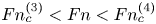 $Fn_c^{(3)}< Fn< Fn_c^{(4)}$ are presented in figure 15. For waves under symmetric edges given in figures 15(a), 15(c) and 15(e), there is only one component in the longitudinal wave at the downstream region, while the waves at the upstream region contain two components. It can be found that the wave patterns under clamped–clamped and simply supported–simply supported edges are relatively similar, but the wave pattern under free–free is quite different. In figure 15(e), we can see that the downstream wave under free–free edges is not as obvious as that under the other two symmetric edges. Similar phenomena can be also observed from the transverse waves in figures 15(a), 15(c) and 15(e). From these results, we may infer that an ice-covered channel with free–free edges is closer to an unbounded region when compared with those with other edge constraints. For waves under asymmetric edge constraints shown in figures 15(b), 15(d) and 15(f). The longitudinal waves at the downstream region consist of two components, while the waves at the upstream region contains three components. Compared with the wave profiles under clamped–simply supported edges shown in figure 15(b), the asymmetry of the transverse waves is more obvious in cases with a free edge given in figures 15(d) and 15(f).

Figure 13. Hydrodynamic forces on the cylinder in an ice-covered channel with free–free edges at different channel widths: (a) resistance; (b) lift.

Figure 14. Ice sheet deflection  $\eta$ along
  $x$-axis due to a submerged horizontal cylinder when the ice sheet is under clamped–clamped edges: (a)
  $Fn< Fn_c^{(1)}$; (b)
  $Fn_c^{(1)}< Fn< Fn_0$; (c)
  $Fn_c^{(2)}< Fn< Fn_c^{(3)}$; (d)
  $Fn_c^{(4)}< Fn< Fn_c^{(5)}$; with
  $Fn_c^{(1)}=0.8180$,
  $Fn_c^{(2)}=0.9981$,
  $Fn_c^{(3)}=1.3177$,
  $Fn_c^{(4)}=1.7682$,
  $Fn_c^{(5)}=2.3230$,
  $Fn_0=1.1469$.

Figure 15. Wave patterns under different edge conditions when  $Fn_c^{(3)}< Fn< Fn_c^{(4)}$: (a) clamped–clamped edges,
  $Fn=1.5$ (
 $Fn_c^{(3)}=1.3177$ and
  $Fn_c^{(4)}=1.7682$); (b) clamped–simply supported edges,
  $Fn=1.4$ (
 $Fn_c^{(3)}=1.2569$ and
  $Fn_c^{(4)}=1.6824$); (c) simply supported–simply supported edges,
  $Fn=1.3$ (
 $Fn_c^{(3)}=1.2012$ and
  $Fn_c^{(4)}=1.6005$); (d) clamped-free edges,
  $Fn=1.3$ (
 $Fn_c^{(3)}=1.0962$ and
  $Fn_c^{(4)}=1.4454$); (e) free–free edges,
  $Fn=1.05$ (
 $Fn_c^{(3)}=0.9486$ and
  $Fn_c^{(4)}=1.1997$); (f) simply supported–free edges,
  $Fn=1.1$ (
 $Fn_c^{(3)}=1.0561$ and
  $Fn_c^{(4)}=1.3782$).
5. Conclusions
The interaction of a uniform current with a submerged horizontal circular cylinder in an ice-covered channel is studied analytically, the solution procedure is applicable to various edge conditions. The three-dimensional Green function satisfying all boundary conditions apart from that on the body surface is first derived. By using this, the potential due to sources distributed along the centre line of the cylinder is obtained, from which the potentials due to multipoles are constructed directly by differentiating the position of the centre line. The velocity potential for a submerged circular cylinder is written in terms of a summation of these multipoles.
From the solution of the Green function, it is confirmed that there is an infinite number of critical Froude numbers  $Fn_c^{(i)}$
  $(i=1,2,3\cdots )$ and another one,
  $Fn_0$, which corresponds to the case of
  $Fn_0=1$ in the two-dimensional problem where there are only two critical Froude numbers. This is consistent with what has been noticed in previous work (Khabakhpasheva et al. Reference Khabakhpasheva, Shishmarev and Korobkin2019). There will be no wave propagating to infinity when
  $Fn< Fn_c^{(1)}$. When
  $Fn_c^{(i)}< Fn< Fn_c^{(i+1)}$ and
  $Fn< Fn_0$, there will be
  $2i$ waves, and
  $i$ waves are at a downstream region with group velocity smaller than the current speed, while the other
  $i$ waves with larger group velocity are at an upstream region. When
  $Fn_c^{(i)}< Fn< Fn_c^{(i+1)}$ and
  $Fn>Fn_0$, one downstream wave will disappear, and there will be
  $i-1$ waves at a downstream region. For infinite water depth, the effect of
  $Fn_0$ does not exist. When
  ${\widetilde {Fn}}_c^{(i)}< Fn<{\widetilde {Fn}}_c^{(i+1)}$, there are always
  $2i$ waves, with
  $i$ waves at
  $x=-\infty$ and
  $x=+\infty$, respectively.
In the cases of symmetric edge constraints, the symmetric and antisymmetric transverse modes are completely independent. The former corresponds to the roots of  $Fn=Fn^{(2i-1)}$
  $(i\geq 1)$, while the latter corresponds to the solutions of
  $Fn=Fn^{(2i)}$. If the flow itself is symmetric about
  $y=0$, the waves due to the roots of
  $Fn=Fn^{(2i)}$ will not exist. In general, the symmetric and antisymmetric modes always coexist, and they are fully coupled. When
  $Fn_c^{(i-1)}< Fn< Fn_c^{(i)}$
  $(i\geq 2)$, the contribution of the
  $i$th transverse wave mode to the overall wave profile will be significant.
The ice sheet deflection due to a submerged horizontal circular cylinder shows that the hydroelastic wave is symmetric about  $x=x_0$ and only exists in the region near the cylinder when
  $Fn< Fn_c^{(1)}$. When
  $Fn$ is near
  $Fn_c^{(1)}$, there is a sudden change in the wave above the cylinder, which is similar to that of the two-dimensional case (Li et al. Reference Li, Wu and Shi2019). As
  $Fn$ increases, this phenomenon can be also observed near other critical points which do not exist in the two-dimensional case. The three-dimensional wave pattern also indicates that it can be greatly affected by the edge conditions. The resistance on the cylinder is zero when
  $Fn< Fn_c^{(1)}$, while the lift is non-zero. When
  $Fn$ increases and passes each critical Froude number, the forces change very rapidly. Under different edge conditions, the change is very different.
Acknowledgements
Y.F.Y. is grateful to Lloyd's Register Foundation and China Scholarships Council for sponsoring his PhD study.
Funding
This work is supported by Lloyd's Register Foundation (LRF). The LRF helps protect life and property by supporting engineering-related education, public engagement and the application of research.
Declaration of interests
The authors report no conflict of interest.
Appendix A. Elements of the matrix  $[\boldsymbol {\mathcal {A}}]$ and columns $[\boldsymbol {\mathcal {B}}]$ and $[C]$ under the clamped–clamped edge condition


Applying the clamped–clamped edge condition shown in (2.11) to  $\xi$, we have
 \begin{equation} \left.\begin{gathered} c_0-bc_1+b^2c_2-b^3c_3+\frac{a_0}{24}b^4+\sum_{m=1}^{+\infty}\frac{a_m}{\sigma_m^4}=0\\ c_1-2bc_2+3b^2c_3-\frac{a_0}{6}b^3=0\\ c_0+bc_1+b^2c_2+b^3c_3+\frac{a_0}{24}b^4+\sum_{m=1}^{+\infty}({-}1)^m\frac{a_m}{\sigma_m^4}=0\\ c_1+2bc_2+3b^2c_3+\frac{a_0}{6}b^3=0 \end{gathered} \right\}. \end{equation}
Substituting (3.15) and (3.18a) into (A1), the coefficients of matrix  $[\boldsymbol {\mathcal {A}}]$ and column
  $[\boldsymbol {\mathcal {B}}]$ can then be given as
 \begin{equation} \left.\begin{gathered} \mathcal{A}_{0j}=\delta_{0j}-\delta_{1j}b+\delta_{2j}b^2-\delta_{3j}b^3+ \frac{\alpha_{0,j}}{24}b^4+\sum_{m=1}^{+\infty}\frac{\alpha_{m,j}}{\sigma_m^4}\\ \mathcal{A}_{1j}=\delta_{1j}-\delta_{2j}2b+\delta_{3j}3b^2-\frac{\alpha_{0,j}}{6}b^3\\ \mathcal{A}_{2j}=\delta_{0j}+\delta_{1j}b+\delta_{2j}b^2+\delta_{3j}b^3+ \frac{\alpha_{0,j}}{24}b^4+\sum_{m=1}^{+\infty}({-}1)^m\frac{\alpha_{m,j}}{\sigma_m^4}\\ \mathcal{A}_{3j}=\delta_{1j}+\delta_{2j}2b+\delta_{3j}3b^2+\frac{\alpha_{0,j}}{6}b^3 \end{gathered}\right\}, \end{equation}
 \begin{equation} \mathcal{B}_j={-}\text{i}\sum_{m=0}^{+\infty} \frac{\rho Uk\cosh K_m(z_0+H)\cos\sigma_m(y_0+b)}{(1+\delta_{m0})b\varDelta_m \cosh K_mH}\nu_{m,j},\quad j=0\sim3, \end{equation}
where
 \begin{equation} \nu_{m,j}=\left\{\begin{aligned} & \delta_{0j}\left[\frac{1-\delta_{m0}}{\sigma_m^4}+\delta_{m0} \left(\frac{b^4}{24}+\sum_{l=1}^{+\infty}\frac{\gamma_l}{\sigma_l^4}\right)\right]-\delta_{1j} \delta_{m0}\frac{b^3}{6}\\ & \quad +\delta_{2j}\left[\frac{(1-\delta_{m0})({-}1)^m}{\sigma_m^4}+\delta_{m0}\left(\frac{b^4}{24}+ \sum_{l=1}^{+\infty}\frac{({-}1)^l\gamma_l}{\sigma_l^4}\right)\right]+\delta_{3j}\delta_{m0}\frac{b^3}{6} \end{aligned}\right\}. \end{equation}
Based on (A2) and (A3), the solution of  $c_i$ of (3.21) can be obtained as
 \begin{equation} c_i ={-}\text{i}\sum_{m=0}^{+\infty}\frac{\rho Uk\cosh K_m(z_0+H)\cos \sigma_m(y_0+b)}{(1+\delta_{m0})b|\boldsymbol{\mathcal{A}}|\varDelta_m\cosh K_mH}c_{m,i}^{\prime},\quad i=0\sim3, \end{equation}
where  $c_{m,i}^\prime =|\boldsymbol {\mathcal {A}}|\times c_{m,i}$,
  $c_{m,i}$ is the solution of
  $[\boldsymbol {\mathcal {A}}][\boldsymbol {C_m}]=[\boldsymbol {\nu _m}]$,
  $[\boldsymbol {\nu _m}]$ is a known column containing coefficients
  $\nu _{m,i}$
  $(i=0\sim 3)$,
  $[\boldsymbol {C_m}]$ is an unknown column containing
  $c_{m,i}$.
Substituting (3.20) into (A1), the matrix equation (3.21) can be further split into two  $2\times 2$ submatrices, which can be written as
 \begin{equation}
[\boldsymbol{\mathcal{A}^S}]\left[\begin{array}{@{}c@{}} c_0\\
c_2 \end{array}\right]=[\boldsymbol{\mathcal{B}^S}]\quad
\text{and}\quad
[\boldsymbol{\mathcal{A}^A}]\left[\begin{array}{@{}c@{}} c_1\\
c_3 \end{array}\right]=[\boldsymbol{\mathcal{B}^A}],
\end{equation}
\begin{equation}
[\boldsymbol{\mathcal{A}^S}]\left[\begin{array}{@{}c@{}} c_0\\
c_2 \end{array}\right]=[\boldsymbol{\mathcal{B}^S}]\quad
\text{and}\quad
[\boldsymbol{\mathcal{A}^A}]\left[\begin{array}{@{}c@{}} c_1\\
c_3 \end{array}\right]=[\boldsymbol{\mathcal{B}^A}],
\end{equation}
or symmetric and antisymmetric modes are fully uncoupled. The elements of matrices  $[\boldsymbol {\mathcal {A}^S}]$,
  $[\boldsymbol {\mathcal {A}^A}]$ and columns
  $[\boldsymbol {\mathcal {B}^S}]$,
  $[\boldsymbol {\mathcal {B}^A}]$ can be expressed as
 \begin{equation} \left.\begin{gathered} \mathcal{A}_{0j}^S=\delta_{0j}+\delta_{1j}b^2+ \frac{\alpha_{0,2j}}{24}b^4+\sum_{m=1}^{+\infty}\frac{\alpha_{2m,2j}}{\sigma_{2m}^4}\\ \mathcal{A}_{1j}^S=2\delta_{1j}b+\frac{\alpha_{0,2j}}{6}b^3 \end{gathered}\right\} \end{equation}
and
 \begin{equation} \left.\begin{gathered} \mathcal{A}_{0j}^A=\delta_{0j}b+\delta_{1j}b^3+ \sum_{m=1}^{+\infty}\frac{\alpha_{2m-1,2j+1}}{\sigma_{2m-1}^4}\\ \mathcal{A}_{1j}^A=\delta_{0j}+3\delta_{1j}b^2 \end{gathered}\right\} \end{equation}
and
 \begin{equation} \left.\begin{gathered} \mathcal{B}_j^S={-}\text{i}\sum_{m=0}^{+\infty} \frac{\rho Uk({-}1)^m\cosh K_{2m}(z_0+H)\cos\sigma_{2m}y_0}{(1+\delta_{m0})b\varDelta_{2m} \cosh K_{2m}H}\nu_{m,j}^S\\ \mathcal{B}_j^A=\text{i}\sum_{m=0}^{+\infty}\frac{\rho Uk({-}1)^m\cosh K_{2m+1}(z_0+H) \sin\sigma_{2m+1}y_0}{b\varDelta_{2m+1}\cosh K_{2m+1}H}\nu_{m,j}^A \end{gathered}\right\},\quad j=0,1 \end{equation}
with
 \begin{equation} \nu_{m,j}^S=\delta_{0j}\left[\frac{1-\delta_{m0}}{\sigma_{2m}^4}+\delta_{m0} \left(\frac{b^4}{24}+\sum_{l=1}^{+\infty}\frac{\gamma_{2l}}{\sigma_{2l}^4}\right)\right]+ \delta_{1j}\delta_{m0}\frac{b^3}{6}\quad \text{and} \quad \nu_{m,j}^A=\frac{\delta_{0j}}{\sigma_{2m+1}^4}. \end{equation}
Here  $|\boldsymbol {\mathcal {A}}|$ can be further obtained as
 \begin{equation} |\boldsymbol{\mathcal{A}}|=4|\boldsymbol{\mathcal{A}^S}||\boldsymbol{\mathcal{A}^A}|. \end{equation}
Appendix B. Symmetry property of the Green function
Let  $G_0=G(x,y,z,x_0,y_0,z_0)$ and
  $G_1=G(x,y,z,x_1,y_1,z_1)$, and correspondingly,
  $\xi _0=\xi (x,y,x_0,y_0,z_0)$ and
  $\xi _1=\xi (x,y,x_1,y_1,z_1)$. At
  $x\to +\infty$, the Green function and the wave elevation can be expressed as
 $$\begin{align} G_0 &= \text{Re}\left\{\sum_{j=0}^{S}\frac{G_0^{(\kern0.06em j)}(y,z)}{k_j}\exp({-\text{i}k_j(x-x_0)})\right\}\quad \text{and}\nonumber\\ G_1 &= \text{Re}\left\{\sum_{l=0}^{S}\frac{G_1^{(l)}(y,z)}{k_l}\exp({-\text{i}k_l(x-x_1)})\right\}, \end{align}$$
 $$\begin{align} \xi_0&=\text{Re}\left\{\sum_{j=0}^{S}\xi_0^{(\kern0.06em j)}(y)\exp({-\text{i}k_j(x-x_0)})\right\}\quad \text{and}\nonumber\\ \xi_1&=\text{Re}\left\{\sum_{l=0}^{S}\xi_1^{(l)}(y)\exp({-\text{i}k_l(x-x_1)})\right\}, \end{align}$$
where  $k_0\to 0$ and
  $k_j$
$k_j$  $(\kern0.06em j=1\sim S)$ denote the wavenumber of the component
  $j$, and the summation contains only those wave components with group velocity larger than
  $U$. The terms of
  $j=0$ in (B1a,b) are related to the ‘blockage parameter’, as discussed, for example, in Newman (Reference Newman1969) and Mei & Chen (Reference Mei and Chen1976) in the two-dimensional case. However, for a submerged body, there should be no net flow being created. Therefore, the ‘blockage parameter’ is a constant. Its derivative will be zero and no flow will be created by the constant. Equation (B1a,b) is due to a source which does generate flow into the fluid domain. This will continue at infinity, which is reflected by the terms of
  $j=0$ of (B1a,b).
Although  $G$ and
  $\xi$ involve only the real part, we may use the whole complex function here. Substituting (B1a,b) and (B2a,b) into (2.6) and (2.7), the boundary conditions of
  $G_0^{(\kern0.06em j)}$ and
  $\xi _0^{(\kern0.06em j)}$ on ice sheet can be established as
 $$\begin{gather} \text{i }\left[(Lk_j^4+\rho g)\xi_0^{(\kern0.06em j)}-2Lk_j^2 \frac{\text{d}^2\xi_0^{(\kern0.06em j)}}{{\text{d}y}^2}+L\frac{\text{d}^4\xi_0^{(\kern0.06em j)}}{{\text{d}y}^4}\right]= \rho UG_0^{(\kern0.06em j)},\quad j=0\sim S,\enspace z=0, \end{gather}$$
 $$\begin{gather}\text{i}k_j^2U\xi_0^{(\kern0.06em j)}=\frac{\partial G_0^{(\kern0.06em j)}}{\partial z},\quad j=0\sim S,\enspace z=0. \end{gather}$$
A similar procedure can be adopted at  $x\to -\infty$. Applying Green's second identity, we have
where  $\mathcal {S}$ is comprised of the seabed
  $S_H$, two vertical channel walls
  $S_w$, ice sheet
  $S_I$ and two vertical surfaces
  $S_{\pm \infty }$ at
  $x\to \pm \infty$, respectively. As
  $\partial G_0/\partial n$ and
  $\partial G_1/\partial n$ are zero on
  $S_H$ and
  $S_w$, only the integrals over
  $S_I$ and
  $S_{\pm \infty }$ need to be kept.
For the integral at  $S_I$, using (2.6), (2.7) and integration by parts, this gives
 \begin{align} I_I&=\iint_{S_I}\left(G_0\frac{\partial G_1}{\partial z}-G_1\frac{\partial G_0}{\partial z}\right)\text{d} S \nonumber\\ &={-}U\int_{{-}b}^{b}\left.\left(G_0\xi_1-G_1\xi_0\right)\right|_{x\to-\infty}^{x\to+\infty}{\text{d}y}+ \frac{L}{\rho}\iint_{S_I}(\xi_1\nabla^4\xi_0-\xi_0\nabla^4\xi_1)\,\text{d} S. \end{align}
Employing (A.3) in Ren et al. (Reference Ren, Wu and Ji2018b),  $I_I$ can be written as
 \begin{align} I_I &={-}U\int_{{-}b}^{b}\left.\left(G_0\xi_1-G_1\xi_0\right)\right|_{x\to-\infty}^{x\to+\infty}{\text{d}y} \nonumber\\ &\quad +\frac{L}{\rho}\oint_{\mathcal{T}}\left(\xi_1\frac{\partial}{\partial n}\nabla^2\xi_0- \frac{\partial \xi_1}{\partial n}\nabla^2\xi_0-\xi_0\frac{\partial}{\partial n}\nabla^2\xi_1+ \frac{\partial \xi_0}{\partial n}\nabla^2\xi_1\right)\text{d} l, \end{align}
where  $\mathcal {T}$ is comprised of the lines
  $x=\pm \infty$ and
  $y=\pm b$. Using (B1a,b)–(B3) and integrating by parts again,
  $I_I$ can be further written as
 \begin{equation}
I_I=\left\{\begin{aligned} &
\frac{\text{i}L}{\rho}\sum_{j=0}^{S}\sum_{l=0}^{S}\exp({-\text{i}[k_j(x-x_0)+k_l(x-x_1)]})\\
&\quad \times \left.\left.\left[\begin{aligned} &
\left(\xi_{1y}^{(l)}\xi_{0yy}^{(\kern0.06em j)}/k_j-\xi_{0y}^{(\kern0.06em j)}\xi_{1yy}^{(l)}/k_l\right)\\
& -\left(\xi_1^{(l)}\xi_{0yyy}^{(\kern0.06em j)}/k_j-\xi_0^{(\kern0.06em j)}\xi_{1yyy}^{(l)}/k_l\right)
\end{aligned}\right]\right|_{y={-}b}^{y=b}\right|_{x\to-\infty}^{x\to+\infty}\\
&\quad
+\frac{L}{\rho}\int_{-\infty}^{+\infty}\left.\left[\begin{aligned}
& \left(\xi_1\xi_{0yyy}-\xi_0\xi_{1yyy}\right)-
\left(\xi_{1y}\xi_{0yy}-\xi_{0y}\xi_{1yy}\right)\\ & \quad
-2\left(\xi_{1x}\xi_{0xy} - \xi_{0x}\xi_{1xy}\right)
\end{aligned}\right]\right|_{y={-}b}^{y=b}{\text{d}\kern0.7pt x}
\end{aligned}\right\} .
\end{equation}
\begin{equation}
I_I=\left\{\begin{aligned} &
\frac{\text{i}L}{\rho}\sum_{j=0}^{S}\sum_{l=0}^{S}\exp({-\text{i}[k_j(x-x_0)+k_l(x-x_1)]})\\
&\quad \times \left.\left.\left[\begin{aligned} &
\left(\xi_{1y}^{(l)}\xi_{0yy}^{(\kern0.06em j)}/k_j-\xi_{0y}^{(\kern0.06em j)}\xi_{1yy}^{(l)}/k_l\right)\\
& -\left(\xi_1^{(l)}\xi_{0yyy}^{(\kern0.06em j)}/k_j-\xi_0^{(\kern0.06em j)}\xi_{1yyy}^{(l)}/k_l\right)
\end{aligned}\right]\right|_{y={-}b}^{y=b}\right|_{x\to-\infty}^{x\to+\infty}\\
&\quad
+\frac{L}{\rho}\int_{-\infty}^{+\infty}\left.\left[\begin{aligned}
& \left(\xi_1\xi_{0yyy}-\xi_0\xi_{1yyy}\right)-
\left(\xi_{1y}\xi_{0yy}-\xi_{0y}\xi_{1yy}\right)\\ & \quad
-2\left(\xi_{1x}\xi_{0xy} - \xi_{0x}\xi_{1xy}\right)
\end{aligned}\right]\right|_{y={-}b}^{y=b}{\text{d}\kern0.7pt x}
\end{aligned}\right\} .
\end{equation}
Invoking the edge conditions in (2.11), it can be shown  $I_I=0$ for any of these edge constraints.
For the integral over  $S_{\pm \infty }$, we can consider
  $S_{+\infty }$ as an example, as the integral over
  $S_{-\infty }$ can be done in a similar way. Substituting (B1a,b) into the integral at
  $S_{+\infty }$, we have
 \begin{align} I_{+\infty}&=\iint_{S_{+\infty}}\left(G_0\frac{\partial G_1}{\partial x}-G_1 \frac{\partial G_0}{\partial x}\right)\text{d} S \nonumber\\ &=\sum_{j=0}^{S}\sum_{l=0}^{S}\exp({-\text{i}[k_j(x-x_0)+k_l(x-x_1)]}) \iint_{S_{+\infty}}\left(\frac{1}{k_l}-\frac{1}{k_j}\right)G_0^{(\kern0.06em j)}G_1^{(l)}\,\text{d} S. \end{align}
Since  $G_0$ and
  $G_1$ is governed by the Laplace equation at
  $x\to +\infty$, we have
 \begin{equation} \left.\begin{gathered} \nabla_{yz}^2G_0^{(\kern0.06em j)}=k_j^2G_0^{(\kern0.06em j)}\\ \nabla_{yz}^2G_1^{(l)}=k_j^2G_1^{(l)} \end{gathered}\right\}, \end{equation}
where  $\nabla _{yz}^2=\partial ^2/\partial y^2+\partial ^2/\partial z^2$ denotes the Laplace operator on the
  $O-yz$ plane. Substituting (B10) into (B9) and applying Green's second identity, we obtain
 \begin{align} I_{+\infty}&=\text{i}\sum_{j=0}^{S}\sum_{l=0}^{S} \frac{\exp({-\text{i}[k_j(x-x_0)+k_l(x-x_1)]})}{k_jk_l(k_j+k_l)} \iint_{S_{+\infty}}\left(G_1^{(l)}\nabla_{yz}^2G_0^{(\kern0.06em j)}-G_0^{(\kern0.06em j)} \nabla_{yz}^2G_1^{(l)}\right)\text{d} S \nonumber\\ &=\text{i}\sum_{j=0}^{S}\sum_{l=0}^{S}\frac{\exp({-\text{i}[k_j(x-x_0)+k_l(x-x_1)]})}{k_jk_l(k_j+k_l)} \oint_{\mathcal{L}_{+\infty}}\left(G_1^{(l)}\frac{\partial G_0^{(\kern0.06em j)}}{\partial n}-G_0^{(\kern0.06em j)} \frac{\partial G_1^{(l)}}{\partial n}\right)\text{d} S, \end{align}
where  $\mathcal {L}_{+\infty }$ is comprised of lines
  $y=\pm b$,
  $z=0$ and
  $z=-H$. Applying (2.9), (2.10), (B3) and (B4), we have
 \begin{align} I_{+\infty} &= \frac{\text{i}L}{\rho}\sum_{j=0}^{S}\sum_{l=0}^{S} \frac{\exp({-\text{i}[k_j(x-x_0)+k_l(x-x_1)]})}{k_l+k_j} \nonumber\\ &\quad \times\int_{{-}b}^{{+}b} \left[\begin{aligned} & \quad 2k_jk_l\left(\xi_0^{(\kern0.06em j)}\xi_{1yy}^{(l)}-\xi_1^{(l)}\xi_{0yy}^{(\kern0.06em j)}\right)\\ & -\left(k_j\xi_0^{(\kern0.06em j)}\xi_{1yyyy}^{(l)}/k_l-k_l\xi_1^{(l)}\xi_{0yyyy}^{(\kern0.06em j)}/k_j\right) \end{aligned}\right]{\text{d}y}. \end{align}
Using integration by parts and edge conditions in (2.11), we have  $I_{+\infty }=0$, similarly
  $I_{-\infty }=0$. This means that the integral at right-hand side of (B5) is equal to
  $0$, which gives
 \begin{equation} G\left(x_1,y_1,z_1,x_0,y_0,z_0\right)=G\left(x_0,y_0,z_0,x_1,y_1,z_1\right). \end{equation}
Appendix C. Far-field formula of the resistance
The formula of the resistance can be written as (Wu Reference Wu1995)
 \begin{equation} F_R={-}\frac{1}{2}\rho\iint_{S_B}\left(\phi_x\frac{\partial\phi}{\partial n}-\phi \frac{\partial\phi_x}{\partial n}\right)\text{d} S. \end{equation}
Using Green's second identity, it can be converted to
 \begin{equation} F_R=\frac{1}{2}\rho\iint_{S_I+S_{{\pm}\infty}}\left(\phi_x\frac{\partial\phi}{\partial n}-\phi \frac{\partial\phi_x}{\partial n}\right)\text{d} S. \end{equation}
It is noted that the integral in (C2) can be treated in a similar way as shown in Appendix B. This gives
 \begin{equation} F_R=\left[\begin{aligned} & \frac{1}{2}\rho\int_{{-}H}^{0}\text{d} z\int_{{-}b}^{b}\left.\left(\frac{\partial\phi}{\partial x} \frac{\partial\phi}{\partial x}-\phi\frac{\partial^2\phi}{\partial x^2}\right)\right|_{x\to-\infty}^{x\to+\infty}{\text{d}y}\\ & \quad -\frac{1}{2}\rho U\int_{{-}b}^{b}\left.\left.\left(\eta\frac{\partial \phi}{\partial x}-\phi \frac{\partial \eta}{\partial x}\right)\right|_{x\to-\infty}^{x\to+\infty}\right|_{z=0}{\text{d}y}\\ & \quad +\frac{L}{2}\int_{{-}b}^{b}{\left.\left[\left(\eta\frac{\partial^4\eta}{\partial x^4}- \frac{\partial\eta}{\partial x}\frac{\partial^3\eta}{\partial x^3}\right)- \left(\frac{\partial\eta}{\partial x}\frac{\partial^3\eta}{\partial x^3}- \frac{\partial^2\eta}{\partial x^2}\frac{\partial^2\eta}{\partial x^2}\right)\right]\right|_{x\to-\infty}^{x\to+\infty}{\text{d}y}}\\ & \quad +\frac{L}{U}\int_{{-}b}^{b}{\left.\left(\eta\frac{\partial^4\phi}{\partial x^3\partial z}+ \eta\frac{\partial\phi}{\partial x\partial z^3}-\frac{\partial\eta}{\partial x} \frac{\partial^3\phi}{\partial x^2\partial z}-\frac{\partial\eta}{\partial x} \frac{\partial\phi}{\partial z^3}\right)\right|_{x\to-\infty}^{x\to+\infty}{\text{d}y}} \end{aligned}\right]. \end{equation}
Based on (3.40) and (3.53), the asymptotic expression of  $\phi$ and
  $\eta$ at
  $x\to +\infty$ can be written as
 \begin{align}
\phi&=\text{Re}\left\{\sum_{s=1}^{S}\sum_{n=0}^{+\infty}\chi_s
\frac{\begin{array}{l}\left[\mathscr{B}_{s,n}^{(1)}\exp({\text{i}k_s(x-x_0)})+
\mathscr{B}_{s,n}^{(2)}\exp({-\text{i}k_s(x-x_0)})\right]\\ \quad \times k_s\cosh
K_{n,s}(z+H) \cos\sigma_n(y+b)\end{array}}{K_{n,s}\sinh
K_{n,s}H}\right\} \nonumber\\ &\quad
+\text{sgn}(x)\phi^{(0)}, \end{align}
\begin{align}
\phi&=\text{Re}\left\{\sum_{s=1}^{S}\sum_{n=0}^{+\infty}\chi_s
\frac{\begin{array}{l}\left[\mathscr{B}_{s,n}^{(1)}\exp({\text{i}k_s(x-x_0)})+
\mathscr{B}_{s,n}^{(2)}\exp({-\text{i}k_s(x-x_0)})\right]\\ \quad \times k_s\cosh
K_{n,s}(z+H) \cos\sigma_n(y+b)\end{array}}{K_{n,s}\sinh
K_{n,s}H}\right\} \nonumber\\ &\quad
+\text{sgn}(x)\phi^{(0)}, \end{align}
 \begin{align} \eta &={-}\frac{1}{U}\text{Im}\left\{\sum_{s=1}^{S}\sum_{n=0}^{+\infty}\chi_s [\mathscr{B}_{s,n}^{(1)}\exp({\text{i}k_s(x-x_0)}) \right.\nonumber\\ &\quad \left.\vphantom{\sum_{s=1}^{S}\sum_{n=0}^{+\infty}} -\mathscr{B}_{s,n}^{(2)}\exp({-\text{i}k_s(x-x_0)})]\cos\sigma_n(y+b)\right\}, \end{align}
where
 \begin{equation} \left.\begin{gathered} \mathscr{B}_{s,n}^{(1)}={-}\text{i}\rho U\sum_{n^{\prime}=0}^{+\infty} \sum_{m=1}^{+\infty}\frac{r_0^mf_{n^{\prime},m}\tau_{n,n^{\prime}} (k_s)E_{n^{\prime},m}(k_s,z_0)}{2^m(m-1)!\varDelta_{n^{\prime}}(k_s)|\boldsymbol{\mathcal{A}}|^{\prime}(k_s)\cosh K_{n^{\prime},s}H}\\ \mathscr{B}_{s,n}^{(2)}=\text{i}\rho U\sum_{n^{\prime}=0}^{+\infty} \sum_{m=1}^{+\infty}\frac{r_0^mf_{n^{\prime},m}\tau_{n,n^{\prime}} (k_s)E_{n^{\prime},m}({-}k_s,z_0)}{2^m(m-1)!\varDelta_{n^{\prime}}(k_s)|\boldsymbol{\mathcal{A}}|^{\prime}(k_s)\cosh K_{n^{\prime},s}H} \end{gathered}\right\} \end{equation}
and where  $K_{n,s}=\sqrt {k_s^2+\sigma _n^2}$,
  $\tau _{n,n^{\prime }}(k)=\sum _{j=0}^{3}\beta _{n,j}c_{n^{\prime },j}^{\prime }$, and the summation of
  $s$ contains only those wave components with group velocity larger than
  $U$. Here
  $\chi _s$ is related to the integration path
  $\mathscr {L}$ in (3.38c) and (3.55c), when
  $\mathscr {L}$ passes over (under) the singularity at
  $k_s$, the corresponding wave component will propagate to
  $x=+\infty$ (
 $x=-\infty$), and
  $\chi _s=-1$ (
 $\chi _s=+1$). Therefore,
  $\chi _s=-1$ in (C4) and (C5). Similar procedure can be also adopted at
  $x\to -\infty$. Substituting (C4) and (C5) into (C3), we have
 \begin{align} F_R &={-}\frac{b}{4U^2}\sum_{s=1}^{S}\sum_{n=0}^{+\infty}(1+\delta_{n0})\chi_s \left|\mathscr{B}_{s,n}^{(1)}+\bar{\mathscr{B}}_{s,n}^{(2)}\right|^2 \nonumber\\ &\quad \times \left[\begin{aligned} & \rho U^2k_s^2\left(H+\sinh 2K_{n,s}H/2K_{n,s}\right)\\ & \quad -\rho U^2K_{n,s}\sinh{2K_{n,s}H}\\ & \quad +4LK_{n,s}^4\sinh^2K_{n,s}H \end{aligned}\right]. \end{align}
It should be noted that the summation of  $s$ in (C7) contains all the wave components.


