


1. Introduction
In the field of reliability research, redundancy allocation is widely used to improve the reliability of a system. In general, there is a important type of redundancy known as active redundancy commonly used in reliability engineering and system security. Active redundancy means that spares have been attached in parallel to components of system and they start functioning at the same time as original components. The research of this topic is mainly divided into two levels: active redundancy at the component level ( ${\rm ARCL}$) and at the system level (
 ${\rm ARSL}$). In the former case, the main problem is where to allocate active spares in a system to improve the reliability; see, for example, Boland et al. [Reference Boland, El-Neweihi and Proschan6], Li and Ding [Reference Li and Ding25], Li et al. [Reference Li, Yan and Hu27], Zhao et al. [Reference Zhao, Chan and Ng52], Zhuang and Li [Reference Zhuang and Li54], You et al. [Reference You, Fang and Li48], Fang and Li [Reference Fang and Li12,Reference Fang and Li13], Chen et al. [Reference Chen, Zhang, Zhao and Zhou8], Yan and Luo [Reference Yan and Luo43], You and Li [Reference You and Li47], Zhang [Reference Zhang49], Ling et al. [Reference Ling, Wei and Li28], Yan et al. [Reference Yan, Lu and Li45], Kim [Reference Kim21], Navarro et al. [Reference Navarro, Fernández-Martínez, Fernández-Sánchez and Arriaza36] and Zhang et al. [Reference Zhang, Zhang and Fang51]. In the later case, Barlow and Proschan [Reference Barlow and Proschan1] first proposed a well-known BP principle that
  ${\rm ARCL}$ is more reliable
  ${\rm ARSL}$ in the sense of usual stochastic ordering for the coherent system with independent components. Over the past few decades, more and more researchers have been digging into the related problems, including whether the BP principle still holds for other stronger stochastic orders, and what effect of dependence among components on BP principle. This study can be divided into three aspects: (1) complete matching, in which all spares and components are identical; (2) matching, in which only the coupled spares and the original components are identical and (3) nonmatching, none of coupled spares has the same distribution as the original components. Based on the assumption that among original components, among spares, and spares and original components are all independent, for complete matching, Boland and El-Neweihi [Reference Boland and El-Neweihi5], Singh and Singh [Reference Singh and Singh41] and Gupta and Nanda [Reference Gupta and Nanda15] have extended the BP principle to the (reversed) hazard rate order and the likelihood ratio order. For matching case, Misra et al. [Reference Misra, Dhariyal and Nitin30], Hazra and Nanda [Reference Hazra and Nanda17] and the references therein devoted to enhance the BP principle to the (reversed) hazard rate order, the likelihood ratio order, and some shifted stochastic orders. However, due to the complexity of distribution theory, there are few results for the case of nonmatching. Misra et al. [Reference Misra, Dhariyal and Nitin30] established the BP principle in the sense of the reversed hazard rate order for coherent system with independent identical distributed (i.i.d.) components. Hazra and Nanda [Reference Hazra and Nanda17] and Kuiti et al. [Reference Kuiti, Hazra and Finkelstein24] showed that the BP principle holds in the reversed hazard rate order and the stochastic precedence order for
  $k$-out-of-
 $n$ system with i.i.d. components.
In the past years, under the assumptions that spares are dependent identical distributed (d.i.d.) and independent of original components, some scholars have devoted to study the BP principles of systems with d.i.d. original components. For example, in the case of matching and nonmatching, Gupta and Kumar [Reference Gupta and Kumar14] firstly gave some sufficient or necessary conditions to compare  ${\rm ARCL}$ and
  ${\rm ARSL}$ in sense of the likelihood ratio, (reversed) hazard rate, and usual stochastic orders for a general coherent system. Furthermore, for the case of complete matching and nonmatching, based on the framework of possibly heterogeneous multiple redundancy hypothesis, Zhang et al. [Reference Zhang, Amini-Seresht and Ding50] further employed various stochastic orders to study this topic. Recently, based on the work of Zhang et al. [Reference Zhang, Amini-Seresht and Ding50], for the case of matching and nonmatching, Yan and Wang [Reference Yan and Wang44] extended the BP principle from d.i.d. original components to dependent nonidentical distributed (d.n.i.d.) components. For more research of the BP principle, refer to Boland and El-Neweihi [Reference Boland and El-Neweihi5], Brito et al. [Reference Brito, Zequeira and Valdés7], Nanda and Kamal [Reference Nanda and Kamal31], Zhao et al. [Reference Zhao, Zhang and Li53], Da and Ding [Reference Da and Ding9] and Kuiti et al. [Reference Kuiti, Hazra and Finkelstein23], among others.
The above results obtained in the literature are carried out under the assumption that spares and original components are independent. However, in practice, affected by the common stress level, all spares and components in a resulting system by  ${\rm ARCL}$ or
  ${\rm ARSL}$ may be dependent. Recent years, the research of this issue are lot of attention. Kotz et al. [Reference Kotz, Lai and Xie22] studied bounds for the mean lifetime of the system of a original component and one active redundancy component having positively or negatively dependent lifetimes. For series and parallel systems with one redundancy component, Belzunce et al. [Reference Belzunce, Martínez-Puertas and Ruiz3,Reference Belzunce, Martínez-Puertas and Ruiz4] investigated the optimal allocation policy under the assumption that the redundancy component and the original component are dependent. Jeddi and Doostparast [Reference Jeddi and Doostparast19] employed to study the optimal allocation policy in engineering systems with dependent component lifetime. Recently, Torrado et al. [Reference Torrado, Arriaza and Navarro42] studies the effect of redundancies on the reliability of coherent systems formed by modules, including active redundancy at components’ level versus redundancies at modules’ level. In particularly, under the assumption of dependent components within the modules and dependent modules, they compare the reliability functions of systems formed by possibly dependent modules consisting of heterogeneous components with redundancies at components’ or modules’ levels.
In addition, researcher often come across the following question: how to measure if one system is aging faster than other systems as time progress, like different brands of mobile phones and different engines made by different companies, the most effective way is relative aging. Relative aging includes aging faster orders in the hazard and reversed hazard rates. Kalashnikov and Rachev [Reference Kalashnikov and Rachev20] provided the notion of aging faster orders in the hazard rate, based on the monotonicity of two hazard rate ratios, and Sengupta and Deshpande [Reference Sengupta and Deshpande39] further proposed the notion of aging faster orders in the reversed hazard rate, based on the monotonicity of two reversed hazard rate ratios. Afterward, Belzunce et al. [Reference Belzunce, Manuel, Ruiz and Carmen Ruiz2], Misra and Francis [Reference Misra and Francis29], Li and Li [Reference Li and Li26], Ding et al. [Reference Ding, Fang and Zhao11] and Ding and Zhang [Reference Ding and Zhang10] made further efforts to enrich those existing results in the literature. Few articles were considered relative agings of resulting systems at the component level and the system level. Hazra and Misra [Reference Hazra and Misra16] not only provided some sufficient conditions for one coherent system to dominate another and a used coherent system and a coherent system made out of used components are compared with respect to aging faster orders, but also, under the assumption that original and redundant components are independent, investigated whether  ${\rm ARCL}$ is more effective than
  ${\rm ARSL}$ with respect to aging faster orders in the case of complete matching, however, this work does not take into account the dependence between components and spares.
To sum up, the work of Zhang et al. [Reference Zhang, Amini-Seresht and Ding50], Hazra and Misra [Reference Hazra and Misra16] and Yan and Wang [Reference Yan and Wang44] were derived within the context of independence between spares and original components. As a follow-up, the current article further investigates the case that the vector of the spare lifetimes and the vector of the original component lifetimes are dependent. In this framework, we consider the issue of stochastic comparison of multi-active complete matching and nonmatching spares redundancies at the component level versus the system level, respectively. In particularly, we present some interesting comparison results in the sense of various stochastic orders, and we also obtain two comparison results between relative agings of resulting systems at the component level and the system level, and thus we effectively extended the corresponding conclusions in Zhang et al. [Reference Zhang, Amini-Seresht and Ding50] and Hazra and Misra [Reference Hazra and Misra16] and further efforts to enrich those existing results in the literature.
The rest of this paper is organized as follows. Section 2 introduces some preliminaries. Section 3 gives sufficient conditions under which the lifetimes of  ${\rm ARCL}$ and
  ${\rm ARSL}$ can be compared by means of some stochastic orders and some numerical examples are provided to illustrate the theoretical results. In Section 4, according to editor suggestion, we present an application in engineering. Finally, Section 5 concludes this study. According to the reviewer's suggestion, all proofs are delegated to the Appendix for ease of presentation.
2. Preliminaries
Throughout the article, increasing and decreasing mean nondecreasing and nonincreasing, respectively. Furthermore, the notion “ $a\overset {\textrm {sgn}}{=}b$” means that “
  $a$” and “
 $b$” have the same sign, “
 $=_{\textrm {st}}$” means equality in distribution, and the symbols “
 $\vee$” and “
 $\wedge$” mean the maximum and the minimum, respectively. It is also assumed that random variables mentioned in this paper are nonnegative and absolutely continuous.
Before proceeding to the main results, let us first recall concepts of stochastic orders, relative aging, copula, distorted distribution and the notion of coherent system, which will be used in the sequel.
For a nonnegative random variable  $X$, denote the distribution function, the survival function, the density function, the hazard rate function and the reversed hazard rate function of
  $X$ by
  $F_X$,
  $\bar F_X$,
  $f_X$,
  $h_X$ and
  $\tilde {h}_X$, respectively.
Definition 1 For two random variables  $X$ and
  $Y$,
$Y$,  $X$ is said to be smaller than
  $Y$ in the
(i) usual stochastic order (denoted by
 $X\leq _{\textrm {st}}Y$) if $\bar F_{X}(t)\leq \bar F_{Y}(t)$ for all $t\in (0,\infty )$;
(ii) hazard rate order (denoted by
$X\leq _{\textrm {hr}}Y$) if $\bar F_{Y}(t)/\bar F_{X}(t)$ is increasing in $t\in (0,\infty )$ or, equivalently, if $h_{X}(t)\geq h_{Y}(t)$;(iii) reversed hazard rate order (denoted by
$X\leq _{\textrm {rh}}Y$) if $F_{Y}(t)/F_{X}(t)$ is increasing in $t\in (0,\infty )$ or, equivalently, $\tilde {h}_{X}(t)\leq \tilde {h}_{Y}(t);$(iv) likelihood ratio order (denoted by
$X\leq _{\textrm {lr}}Y$) if $f_{Y}(t)/f_{X}(t)$ is increasing in $t\in (0,\infty )$.


Definition 2 For two random variables  $X$ and
  $Y$,
$Y$,  $X$ is said to be aging faster than
  $Y$ in
(i) the hazard rate (denoted by
$X\prec _c Y$) if $h_X(t)/h_Y(t)$ is increasing on $(0, +\infty )$ [Reference Kalashnikov and Rachev20];(ii) the reversed hazard rate (denoted by
$X\prec _b Y$) if $\tilde {h}_Y(t) /\tilde {h}_X(t)$ is increasing on $(0, +\infty )$ [Reference Rezaei, Gholizadeh and Izadkhah38].


The following implications are well known (see Theorem 1.C.4. in [Reference Shaked and Shantikumar40])
(i)
$X\leq _{\textrm {lr}} Y \Rightarrow X\leq _{\textrm {hr}}(\leq _{\textrm {rh}})Y\Rightarrow X\leq _{\textrm {st}} Y$;(ii)
$X\prec _c Y$ + $X\geq _{\textrm {hr}} Y\Rightarrow X\geq _{\textrm {lr}} Y;$(iii)
$X\prec _b Y$ + $X\leq _{\textrm {rh}} Y\Rightarrow X\leq _{\textrm {lr}} Y$.


For more details of stochastic orders and their applications, refer to Shaked and Shantikumar [Reference Shaked and Shantikumar40].
Definition 3 A copula is a function  $C:I^{n}\to I$ with the following properties:
(i)
$C(v_1,v_2\ldots v_n)$ is increasing in $v_i,\ i=1,2,\ldots ,n,$(ii)
$C(1,\ldots ,1, v_i,1,\ldots 1)=v_i,$ for all $i=1,2,\ldots ,n,$(iii)
$C(0,\ldots ,0)=0$ and $C(1,\ldots ,1)=1,$ and(iv) for any
$x_1,x_2,\ldots ,x_n$, $y_1,y_2,\ldots ,y_n,$ if $x_j\leq y_j$, $j=1,2,\ldots ,n,$ then
where$$\sum_{i_1=1}^{2}\sum_{i_2=1}^{2}\cdots\sum_{i_n=1}^{2}({-}1)^{i_1+i_2+\cdots+i_n}C(v_{1i_1},u_{2i_2},\ldots, v_{ni_n}),$$
$v_{j1}=x_j,v_{j2}=y_j$, $j=1,2,\ldots ,n$.


The following Lemma is very useful in sequel.
Lemma 1 ([Reference Nelsen37])
Let  $C:I^{n}\to I$ be a copula. Then, for any
  $v_j\in [0,1]$,
 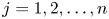 $j=1,2,\ldots ,n$, the partial derivative
  $\partial C(v_1,v_2,\ldots ,v_n)/\partial v_i$ exits for almost all
  $v_i\ (i\neq j=1,2,\ldots ,n),$ and for such
  $v_i\ (i=1,2,\ldots ,n),$
 \begin{equation} 0\leq\frac{\partial C(v_1,v_2,\ldots,v_n)}{\partial v_i}\leq 1. \end{equation}
In particular, when  $v_1=v_2=\cdots =v_n=v,$ denote
  $\beta _{n}(v)=C(v,v,\ldots ,v),$ for all
  $v\in (0,1)$. For more details of copula, refer to Nelsen [Reference Nelsen37].
A system is called a coherent system, if the system structure function is increasing in each component and all components in the system are relevant. In other words, an improvement of a component cannot lead to a deterioration in the performance of the system.
For a general coherent system with  $n$ dependent heterogeneous components having lifetimes
  $X_1,\ldots ,X_n,$ let
 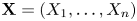 $\textbf {X}=(X_1,\ldots ,X_n)$, and denote
  $F,$
$F,$  $\bar F$ and
  $f$ the distribution function, the survival function and the density function of
  $X_i\ (i=1,2,\ldots ,n$), respectively. Then, the joint distribution function of
  $\mathbf {X}$ can be expressed as
 \begin{equation} H(x_1,\ldots,x_n)=P(X_1\leq x_1,\ldots,X_n\leq x_n)= C (F(x_1),\ldots, F(x_n)), \end{equation}
where  $C$ is a copula of
  $X_1,\ldots ,X_n$. Denote
  $\tau (\textbf {X})$ the lifetime of the coherent system. Then, according to Navarro et al. [Reference Navarro, Aguila, Sordo and Suárez-Llorens34], the survival function of
  $\tau (\textbf {X})$ is
 \begin{equation} \bar H_{\tau (\textbf{X})}(x)=P(\tau (\textbf{X})>x)=q(\bar F(x)),\quad x\geq 0, \end{equation}
where 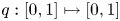 $q:[0,1]\mapsto [0,1]$ is the distortion function of the system, which is increasing continuous and satisfies
  $q(0)=0$, and
  $q(1)=1$, and depends only on the structure function of the system and the survival copula of components.
For more details about distorted distribution, refer to Navarro and Durante [Reference Navarro and Durante32] and Navarro et al. [Reference Navarro and Durante32].
3. Main results
3.1. System description
Consider a coherent system  ${\rm SO}$ composed of
  $n$ d.i.d. components
 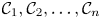 $\mathcal {C}_{1}, \mathcal {C}_{2}, \ldots , \mathcal {C}_{n}$. Denote
  $X_i$ the random lifetime of
  $\mathcal {C}_{i}$ (
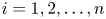 $i=1,2,\ldots , n$), and
  $F_1$ the
  ${X}'_i$s common distribution function. For
  $mn$ dependent spares
  $R_{11},R_{12},\ldots , R_{1n}$;
  $R_{21},R_{22},\ldots , R_{2n}$;
  $\ldots ;$
  $R_{m1}, R_{m2},\ldots , R_{mn}$, denote
  $Y_{j1},Y_{j2},\ldots ,Y_{jn}$ the random lifetimes of spares
  $R_{j1},R_{j2},\ldots ,R_{jn}$, respectively
  $(j=1,2,\ldots ,m)$. Suppose that
  $Y_{j1},Y_{j2},\ldots ,Y_{jn}$ have the common distribution function
  $F_{j+1}\ (j=1,2,\ldots ,m)$. To improve the reliability of the coherent system, we can implement
  ${\rm ARCL}$ or
  ${\rm ARSL}$ for the system. For
  ${\rm ARCL}$, we first allocate the spares
  $R_{1i},R_{2i},\ldots , R_{mi}$ to component
  $\mathcal {C}_{i}$ by active redundancy and form a subsystem with lifetime
 $${\rm SP}_{i}=X_{i}\vee Y_{1i}\vee\cdots\vee Y_{mi},\quad i=1,2,\ldots,n.$$
And then  ${\rm SP}_{1}, {\rm SP}_{2}, \ldots , {\rm SP}_{n}$ can result in a new system having the same structure with the original system. Suppose that the lifetime of the coherent system
  ${\rm SO}$ is
  $\tau (X_1, X_2, \ldots , X_n)$, and thus the lifetime of the resulting system at
  ${\rm ARCL}$ can be expressed as
 \begin{align} \tau_{\rm ARCL}& =\tau({\rm SP}_1, {\rm SP}_2, \ldots, {\rm SP}_n)\nonumber\\ & =\tau(X_1\vee Y_{11}\vee \cdots\vee{Y}_{m1}, X_2\vee Y_{12}\vee \cdots\vee{Y}_{m2}, \ldots,X_n\vee Y_{1n}\vee \cdots\vee{Y}_{mn}). \end{align}
For  ${\rm ARSL}$, by copying the original coherent system structure, for any
  $j\ (j=1,2,\ldots ,m)$, we can obtain a coherent subsystem
  ${\rm SQ}_j$ composed of spares
  $R_{j1},R_{j2},\ldots ,R_{jn},$ and further form the parallel system of
  ${\rm SO}$,
  ${\rm SQ}_1, {\rm SQ}_2, \ldots , {\rm SQ}_m$. Consider that the lifetime of the system
  ${\rm SQ}_j$ is
  $\tau (Y_{j1},Y_{j2},\ldots ,Y_{jn})\ (j=1,2,\ldots ,m)$, then the lifetime of the resulting system at
  ${\rm ARSL}$ can be written as
 \begin{equation} \tau_{\rm ARSL}={\vee}\{\tau(X_1, X_2, \ldots, X_n), \tau(Y_{11},Y_{12},\ldots,Y_{1n}), \ldots, \tau(Y_{m1},Y_{m2},\ldots,Y_{mn}) \}. \end{equation}
Affected by the common stress level, all spares and components in a resulting system by  ${\rm ARCL}$ or
  ${\rm ARSL}$ may be dependent. For simplicity, throughout the paper, we always suppose that
  ${\rm SP}_1,{\rm SP}_2,\ldots ,{\rm SP}_n$;
  $Y_{j1},Y_{j2},\ldots ,Y_{jn}$
  $(j=1,2,\ldots ,m)$ and
  $X_1, X_2,\ldots ,X_n$ have the common copula
  $C'$, and
  $X_i,Y_{1i},Y_{2i},\ldots ,Y_{mi}\ (i=1,2,\ldots ,n)$ and
  ${\rm SO},\, {\rm SQ}_1, {\rm SQ}_2, \ldots , {\rm SQ}_m$ also have the common copula
  $C$. Then, in the case of noncomplete matching, the survival functions of
  ${\rm ARCL}$ and
  ${\rm ARSL}$ can be expressed as
 $$\bar F_{\rm ARCL}(u_1,u_2,\ldots,u_{m+1})=P(\tau_ {\rm ARCL}>t)= q(1-C(u_1,u_2,\ldots,u_{m+1}))$$
and
 \begin{align*} & \bar F_{\rm ARSL}(u_1,u_2,\ldots,u_{m+1})\\ & \quad =P(\tau_{\rm ARSL}>t)=1-C(1- q(1-u_1),1-q(1-u_2),\ldots,1- q(1-u_{m+1})), \end{align*}
respectively. Where the distortion function  $q$ depend on the system structure and copula
  $C'$. In the complete matching case, note that
  $u_1=u_2=\cdots =u_{m+1}=u,$ hence the survival functions of
  ${\rm ARCL}$ and
  ${\rm ARSL}$ are given by
 $$\bar F_{\rm ARCL}(u)= q(1- \beta_{m+1}(u))$$
and
 $$\bar F_{\rm ARSL}(u)=1- \beta_{m+1}(1- q(1-u)),$$
respectively.
From convenience, for a differentiable function  $f$, define
 $$K_f(x)=\frac{xf'(x)}{f(x)},\quad L_f(x)=\frac{(1-x){f'(x)}}{1-f(x)}.$$
3.2. Complete matching case
In this subsection, we discuss the case of coherent system with d.i.d. components and multiple spares. For the coherent system with d.i.d. components and spares, within independence between spares and original components, assuming that  $q(2p-p^{2})\geq 2q(p)-(q(p))^{2}$, Gupta and Kumar [Reference Gupta and Kumar14] proved that
 \begin{equation} \tau_{\rm ARCL}\geq_{\textrm{st}} \tau_{\rm ARSL}, \end{equation}
which means that  ${\rm ARCL}$ is better than
  ${\rm ARSL}$ in the sense of the usual stochastic ordering for a coherent system. However, the spares and original components may be dependent. Therefore, the independence between spares and original components assumption in Eq. (6) seems unreasonable in some practical scenarios. Next, we firstly provide a sufficient condition to show that
  ${\rm ARCL}$ is superior to
  ${\rm ARSL}$ in the sense of the usual stochastic ordering under the assumption of dependence between spares and original components.
Theorem 1 It holds that  $\tau _{\rm ARCL}\geq _{\textrm {st}} \tau _{\rm ARSL},$ if and only if
 \begin{equation} q(1-\beta_{m+1}(u))+\beta_{m+1}(1-q(1-u))\geq 1,\quad \text{for all}\ u\in(0,1). \end{equation}
It should be mentioned that Eq. (6) is just the special case of Theorem 1 if  $m=1$ and
  $\beta _2(u)=u^{2}$.
The following example illustrates that under the condition of Theorem 1,  $\tau _{\rm ARCL}\geq _{\textrm {hr}} \tau _{\rm ARSL}$ or
  $\tau _{\rm ARCL}\geq _{\rm rh} \tau _{\rm ARSL}$ not necessarily holds.
Example 1 Consider a coherent system  $T = \wedge \{X_1,\vee \{X_2, X_3\}\}$ with identical distributed components
  $X_1,X_2$ and
  $X_3$ having Clayton-Oakes (CO) copula
 \begin{equation} C'(v_1,v_2,v_3)=\left(\sum_{i=1}^{3}v^{1-\theta_1}_i-2 \right)^{{1}/{(1-\theta_1)}}, \quad v_i\in[0,1], \end{equation}
where  $\theta _1>1$ is a fixed number. Let
  $Y_{11}$,
  $Y_{12}$ and
  $Y_{13}$ be lifetimes of d.i.d. spares having common survival function and copula (8). Furthermore, suppose
 $$C(v_1,v_2)=\frac{v_1v_2}{1-\theta_2(1-v_1)(1-v_2)},\quad v_i\in[0,1],$$
where  $\theta _2\in [-1,1]$ is a fixed number. Obvious that,
  $m=1$, and taking
  $\theta _1=2, \theta _2={1}/{2}$ then
 $$\beta_2(u)=\frac{2u^{2}}{2-(1-u)^{2}},$$
and the reliability function of this system can be expressed as
 $$q(1-u)=\frac{2-2u}{1+u}-\frac{1-u}{1+2u},$$
and for any  $u\in [0,1]$, it follows from
 \begin{align*} q(1-\beta_{3}(u))+\beta_{3}(1-q(1-u))-1& =\frac{8 (u-1)^{2} u^{3} (21 u^{3}+19 u^{2}+7 u+1)}{(u+1)^{2} (3 u^{2}+2 u+1)({-}u^{4}+36 u^{3}+28 u^{2}+8 u+1)}\\ & \overset{\rm sgn}{=} -u^{4}+36 u^{3}+28 u^{2}+8 u+1\\ & =28 + 36 u - u^{2}\geq 0, \end{align*}
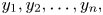
and thus, the condition (7) is satisfied. But Figure 1 shows neither  $\tau _{\rm ARCL}\geq _{\textrm {hr}} \tau _{\rm ARSL}$ nor
  $\tau _{\rm ARCL}\geq _{\textrm {rh}} \tau _{\rm ARSL}$ holds.

Figure 1. Plots of functions  $\bar F_{\rm ARCL}/\bar F_{\rm ARSL}$ and
  ${F}_{\rm ARCL}/{F}_{\rm ARSL}$.
Assuming the independence of spares and original components and the framework of multiple redundancies case, under conditions  ${vq'(v)}/{q(v)}$ is decreasing in
  $v\in (0,1)$ and
  $q(v)\leq v,$ Zhang et al. [Reference Zhang, Amini-Seresht and Ding50] proved that
 \begin{equation} \tau_{\rm ARCL}\geq_{\textrm{hr}} \tau_{\rm ARSL}.\end{equation}
Similarly, the independence between spares and original components assumption in Eq. (9) seems unreasonable in some practical scenarios. Next, we extend corresponding result to the hypothesis of dependence between spares and original components.
Theorem 2 If
(1)
$K_q(1-u)$ is increasing in $u\in (0,1)$,(2)
$L_{\beta _{m+1}}(u)$ is increasing in $u\in (0,1)$ and(3)
$q(1-u)\leq 1-u$ for all $u\in (0,1)$,


then
 $$\tau_{\rm ARCL}\geq_{\textrm{hr}} \tau_{\rm ARSL}.$$
Remark 1 When spares and original components are independent, we have  $\beta _{m+1}(u)=u^{m+1},$ it is obvious that
  $L_{\beta _{m+1}}(u)$ is increasing in
  $u\in (0,1)$ and
  $v=1-u,$ Eq. (9) is just the special case of Theorem 2. Theorem 2 also generalizes Theorem 2 of Gupta and Kumar [Reference Gupta and Kumar14] to the case of dependence of spares and components.
The next numerical example serves as a practical support for the condition required in Theorem 2.
Example 2 Consider a coherent system  $T = \wedge \{X_1,X_2, X_3,X_4\}$ with identical distributed components
  $X_1,X_2,X_3,X_4$ having Gumbel–Barnett copula
  $C'$.
$C'$.
 \begin{equation} C'(v_1,v_2,v_3,v_4)=\left(\prod_{1=1}^{4}v_i\right)e^{-\theta_1\prod_{1=1}^{4}\log v_i}, \quad v_i\in[0,1], \end{equation}
where  $\theta _1>0$. Let
  $Y_{j1}$,
  $Y_{j2}$,
  $Y_{j3}$,
  $Y_{j4}(j=1,2)$ be lifetimes of d.i.d. spares having common survival function and copula (10). Furthermore, suppose
 \begin{equation} C(v_1,v_2,v_3)=\prod_{i=1}^{3}v_i+\theta_2\prod_{i=1}^{3}v_i(1-v_i),\quad v_i\in[0,1], \end{equation}
where  $\theta _2\in [-1,1]$ is a fixed number. Obvious that,
  $m=2$, then,
 $${\beta_3}(u)=u^{3}(1+\theta_2 (1-u)^{3}),$$
and the reliability function of this system can be expressed as
 $$q(1-u)=(1-u)^{4}e^{-\theta_1(\log(1-u))^{4}},$$
and
 \begin{align} K_q(1-u)& = \frac{(1-u)q'(1-u)}{q(1-u)}=4-4 \theta_1 (\log (1-u))^{4},\nonumber\\ {L_{\beta_{3}}}(u)& =\frac{(1-u){\beta_3}'(u)}{1-\beta_3(u)}=\frac{3 u^{2}(\theta_2 (1-2 u) (1-u)^{2}+1)}{-\theta_2 u^{5}+2 \theta_2 u^{4}-\theta_2 u^{3}+u^{2}+u+1}. \end{align}
According to Example 3.13 of Zhang et al. [Reference Zhang, Amini-Seresht and Ding50], we know that  $K_q(1-u)$ is increasing in
  $u$, and
  $q(1-u)\leq 1-u$, for all
  $u\in (0,1)$. It can be verified that the condition (2) in Theorem 2 is satisfied (Appendix A.3). Thus,
  $\tau _{\rm ARCL}\geq _{\textrm {hr}} \tau _{\rm ARSL}$ holds.
The following Theorem 3 gives the reversed hazard rate ordering between  $\tau _{\rm ARCL}$ and
  $\tau _{\rm ARSL}$.
Theorem 3 If
(1)
$K_{\beta _{m+1}}(u)$ is decreasing in $u\in (0,1)$,(2)
$L_q(1-u)$ is decreasing in $u\in (0,1)$ and(3)
$q(1-u)\leq 1-u$ for all $u\in (0,1)$,


then
 $$\tau_{\rm ARCL}\geq_{\textrm{rh}} \tau_{\rm ARSL}.$$
The proof could be completed along the same lines as in Theorem 6, and is hence omitted.
The next numerical example serves as a practical support for the condition required in Theorem 3.
Example 3 Consider a coherent system  $T = \wedge \{X_1,X_2\}$ with identical distributed components
  $X_1$ and
  $X_2$, which have Archimedean copula (see Table 4.1 in [Reference Nelsen37])
 \begin{equation} C'(v_1,v_2)=\max\left\{ \frac{{\theta}^{2}v_1v_2-(1-v_1)(1-v_2)}{{\theta}^{2}-(\theta-1)^{2}(1-v_1)(1-v_2)},0\right\} ,\quad v_1,v_2\in[0,1], \end{equation}
where  $\theta \in [1,\infty ]$ is a fixed number. Let
  $Y_{11}$,
  $Y_{12}$ be lifetimes of d.i.d. spares having common survival function and copula (13). Furthermore, suppose
  $C=C'$. It is obvious that
  $m=1,$ for all
  $\theta \in [1,\infty ],$ we have
 \begin{align*} F_{\rm ARCL}(u)& =1-q(1-\beta_2(u))= \begin{cases} 0, & 0\leq u \leq \dfrac{1}{1+\theta},\\ \dfrac{2 {\theta} ({\theta} u+u-1)}{2 {\theta}^{2}+{\theta} (u-2)+1-u}, & \dfrac{1}{1+\theta}\leq u <\dfrac{1+2\theta^{2}}{1+\theta+2\theta^{2}},\\ 1, & \dfrac{1+2\theta^{2}}{1+\theta+2\theta^{2}}\leq u <1, \end{cases}\\ F_{\rm ARSL}(u)& =\beta_2(1-q(1-u))= \begin{cases} 0, & 0\leq u \leq \dfrac{\theta}{1+\theta+\theta^{2}},\\ \dfrac{2 {\theta}^{2} u+{\theta} (u-1)+u}{2 {\theta}^{2}-{\theta} (u+1)+u}, & \dfrac{\theta}{1+\theta+\theta^{2}}\leq u <\dfrac{\theta}{1+\theta},\\ 1, & \dfrac{\theta}{1+\theta}\leq u <1, \end{cases}\\ L_q(1-u)& =\frac{uq'(1-u)}{1-q(1-u)}=\begin{cases} \dfrac{\theta}{\theta+(\theta-1)u}, & 0\leq u\leq \dfrac{\theta}{1+\theta},\\ 0, & \dfrac{\theta}{1+\theta}< u \leq 1, \end{cases}\\ K_{\beta_{2}}(u)& =\frac{u{\beta_2}'(u)}{{\beta_2}(u)}=\begin{cases} 0, & 0\leq u<\dfrac{1}{1+\theta},\\ \dfrac{2 {\theta}^{2}u}{[1-2\theta-(1-\theta)u][1-(1+\theta)u]}, & \dfrac{1}{1+\theta}\leq u \leq 1, \end{cases} \end{align*}
and
 \begin{align} \Lambda(u)& =\frac{F_{\rm ARCL}(u)}{ F_{\rm ARSL}(u)}\nonumber\\ & =\begin{cases} 0, & 0\leq u<\dfrac{1}{1+\theta},\\ \dfrac{2\theta(2{\theta}^{2}-\theta u+u-\theta)(\theta u+u-1)}{(1-2{\theta}+2{\theta}^{2}-u+\theta u)(2{\theta}^{2}u+\theta u+u-\theta)}, & \dfrac{1}{1+\theta}\leq u <\dfrac{\theta}{1+\theta},\\ 1-q(1-\beta_2(u)), & \dfrac{\theta}{1+\theta}\leq u\leq\dfrac{1+2\theta^{2}}{1+\theta+2\theta^{2}},\\ 1, & \dfrac{1+2\theta^{2}}{1+\theta+2\theta^{2}}\leq u\leq 1. \end{cases} \end{align}
For any  $\theta \in [1,3.2],$ to prove
  $\Lambda (u)$ is increasing in
  $u\in [0,1],$ we just need to prove that
  $\Lambda (u)$ is increasing in
  $u\in [{1}/{(1+\theta )},{\theta }/{(1+\theta )}]$. It is obvious that
  $L_q(1-u)$ is nonnegative and increasing in
  $(1-u)\in [{1}/{(1+\theta )},{\theta }/{(1+\theta )}]$. By Theorem 3, it is sufficient to show that
  $K_{\beta _{2}}(u)$ is decreasing in
  $u\in [{1}/{(1+\theta )},{\theta }/{(1+\theta )}]$. Denote
 $$w_2(u)=\frac{2 {\theta}^{2}u}{[1-2\theta-(1-\theta)u][1-(1+\theta)u]},\quad \frac{1}{1+\theta}\leq u \leq \frac{\theta}{1+\theta}.$$
Note that
 $$w'_2(u)\overset{\rm sgn}{=}({\theta}^{2}-1)u^{2}+1-2\theta,$$
and  $w'_2(0)<0$,
  $w'_2(\sqrt {(2\theta -1)}/{(\theta ^{2}-1)})=0$. It can be verified that
  $\theta \in [1,3.2]$ implies
 $$0<\frac{1} {1+\theta}<\frac{\theta} {1+\theta} <\sqrt\frac{2\theta-1} {\theta^{2}-1},$$
which confirms  $w'_2(u)$ is negative in
  $u\in [{1}/{(1+\theta )},{\theta }/{(1+\theta )}]$. And thus,
  $K_{\beta _{2}}(u)$ is decreasing in
  $u\in [{1}/{(1+\theta )},{\theta }/{(1+\theta )}]$.
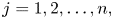
When  $\theta =3.3$, 8, 100, Figure 2(a), (c) and (e) illustrates that the condition (1) of Theorem 3 cannot be satisfied, respectively, and corresponding Figure 2(b), (d) and (f) negates the result of Theorem 3, respectively. It seems that the condition (1) in Theorem 3 be a necessary condition. Unfortunately, we cannot give a mathematical validation.
Remark 2 An insightful reviewer pointed out, whether the conditions of Theorem 3 can be satisfied by the copula in Example 3 for all  $\theta \in [1,\infty ]$. Unfortunately, we give a negative answer as above.

Figure 2. For  $\theta=3.3$, 8, 100, (a)–(c) and (e) plots of the function
  $K_{\beta _2}(u)$, respectively, and (b)–(d) and (f) plots of the function
  $\Lambda^\prime (u)$.
The following example shows that the condition of Theorem 2 do not necessarily imply  $\tau _{\rm ARCL}\prec _c \tau _{\rm ARSL}$ and
  $\tau _{\rm ARCL}\geq _{\textrm {lr}} \tau _{\rm ARSL}$. And thus, the following Theorem 4 gives some condition to strength from
  $\tau _{\rm ARCL}\geq _{\textrm {hr}} \tau _{\rm ARSL}$ to
  $\tau _{\rm ARCL}\prec _c \tau _{\rm ARSL}$ and
  $\tau _{\rm ARCL}\geq _{\textrm {lr}} \tau _{\rm ARSL}$.
Example 4 Consider a coherent system  $T = \wedge \{X_1,\vee \{X_2, X_3\}\}$ with identical distributed components
  $X_1,X_2,X_3$ having Farlie–Gumbel–Morgenstern (FGM) copula
  $C$ (11). Let
  $Y_{j1}$,
  $Y_{j2}$,
  $Y_{j3}(j=1,2)$ be lifetimes of d.i.d. spares having common copula (11). Furthermore, suppose
  $C=C'$. It is obvious that
  $m=2,$ for all
  $\theta \in [1,\infty ],$ we have
 $${\beta_3}(u)=u^{3}(1+\theta (1-u)^{3}),$$
and the reliability function of this system can be expressed as
 $$q(1-u)=2(1-u)^{2} - (1-u)^{3} -\theta u^{3}(1 - u)^{3},$$
and
 \begin{align*} K_q(1-u)& = \frac{(1-u)q'(1-u)}{q(1-u)}=\frac{6 \theta u^{4}-9 \theta u^{3}+3 \theta u^{2}+3 u+1}{\theta u^{4}-\theta u^{3}+u+1},\\ {L_{\beta_{3}}}(u)& =\frac{(1-u){\beta_3}'(u)}{1-\beta_3(u)}=\frac{3 u^{2} (\theta (1-2 u) (1-u)^{2}+1)}{-\theta u^{5}+2 \theta u^{4}-\theta u^{3}+u^{2}+u+1}. \end{align*}
It is obvious that  $K_q(1-u)$ is increasing in
  $u$, and
  $q(1-u)\leq 1-u$, for all
  $u\in (0,1)$ (see Example 3.14 of Zhang et al. [Reference Zhang, Amini-Seresht and Ding50]). According to Example 2, it is obvious that
  $L_{\beta _{3}}(u)$ is increasing in
  $u\in (0,1)$. Thus,
  $\tau _{\rm ARCL}\geq _{\textrm {hr}} \tau _{\rm ARSL}$ holds. Figure 3 illustrates that the relative hazard rate ordering and the likelihood rate ordering do not hold.

Figure 3. For  $\theta =-1$, plots of functions
  $f_{\rm ARCL}/f_{\rm ARSL}$,
  ${h}_{\rm ARCL}/{h}_{\rm ARSL}$ and
  $\bar {F}_{\rm ARCL}/\bar {F}_{\rm ARSL}$.
For the case of complete matching redundancies, when original components independent of spares, suppose that
 $$\left(\frac{(1-q(p))^{m} q'(p)}{1-(1-q(p))^{m+1}}\right)\left(\frac{q(1-(1-p)^{m+1})}{(1-p)^{m} q'(1-(1-p)^{m+1})}\right)$$
is increasing in  $p\in (0,1)$, Hazra and Misra [Reference Hazra and Misra16] proved that
 \begin{equation} \tau_{\rm ARCL}\prec_c \tau_{\rm ARSL}, \end{equation}
and under the conditions that  ${pR'(p)}/{R(p)}$ is decreasing and positive for all
  $p\in (0,1)$, where
  $R(p)=L_q(p),$ they also prove that
 \begin{equation} \tau_{\rm ARCL}\succ _b \tau_{\rm ARSL}. \end{equation}
To make Eqs. (15) and (16) more reasonable in some practical scenarios. Next, we promote the corresponding result in Theorems 4 and 5 to the hypothesis of dependence between spares and original components, respectively.
Theorem 4 If
(1)
$u K'_q(1-u)/{K_q(1-u)}$ is nonpositive and increasing in $u\in (0,1)$,(2)
${u L'_{\beta _{m+1}}(u)}/{ L_{\beta _{m+1}}(u)}$ is positive and decreasing in $u\in (0,1)$ and(3)
$1-q(1-u)\geq uq'(1-u),$ for all $u\in (0,1)$,


then
 $$\tau_{\rm ARCL}\prec_c \tau_{\rm ARSL}$$
and
 $$\tau_{\rm ARCL}\geq_{\textrm{lr}} \tau_{\rm ARSL}.$$
It should be noted that Eq. (15) is just the special case of Theorem 4 if  $\beta _{m+1}(u)=u^{m+1}$ and
  $p=1-u$.
The next numerical example serves as a practical support for the condition required in Theorem 4.
Example 5 Consider a coherent system  $T=\wedge \{X_1,X_2,X_3,X_4\}$ with identical distributed components
  $X_1,X_2,X_3$ and
  $X_4$ having Gumbel–Barnett copula copula
  $C'$ (10). Let
  $Y_{j1}$,
  $Y_{j2}$,
  $Y_{j3}$,
  $Y_{j4}\ (j=1,2,3)$ be lifetimes of d.i.d. spares having common survival function and copula (10). Specifically, we assume
  $C=C'$. It is obvious that
  $m=3,$ then, the reliability function of this system can be represented as
 $$q(1-u)=(1-u)^{4} e^{-\theta \log^{4}(1-u)}.$$
Clearly,
 \begin{align*} {\beta_4}( u)& =u^{4} e^{-\theta \log ^{4}(u)}.\\ {\beta_4}(u)-u{\beta_4}'(u)& =u^{4} e^{-\theta \log ^{4}(u)} [4 \theta \log ^{3}(u)-3],\\ 1-q(u)-(1-u)q'(u)& =e^{-\theta \log ^{4}(u)} [{-}4\theta (u-1) u^{3} \log ^{3}(u)+e^{\theta \log ^{4}(u)}+(3 u-4) u^{3}], \end{align*}
and
 \begin{align*} K_q(1- u) & =4-4 {\theta} \log ^{3}(1-u),\quad L_{\beta_{4}}(u)=\frac{4 (u-1) u^{3} [\theta \log ^{3}(u)-1]}{e^{a \log ^{4}(u)}-u^{4}},\\ \frac{u K'_q(1-u)}{K_q(1-u)}& ={-}\frac{3 \theta u \log ^{2}(1-u)}{(u-1) [\theta \log ^{3}(1-u)-1]},\\ \frac{u L'_{\beta_{4}}(u)}{L_{\beta_{4}}(u)}& =\frac{4 {\theta}^{2} (u-1) \log ^{6}(u) e^{{\theta} \log ^{4}(u)}+{\theta} \log ^{3}(u) [(7-8 u) e^{{\theta} \log ^{4}(u)}+u^{4}]}{(u-1) [u^{4}-e^{{\theta} \log ^{4}(u)}] [{\theta} \log ^{3}(u)-1]}\\ & \quad +\frac{3 {\theta} (u-1) \log ^{2}(u) [u^{4}-e^{{\theta} \log ^{4}(u)}]+(4 u-3) e^{{\theta} \log ^{4}(u)}-u^{4}}{(u-1) [u^{4}-e^{{\theta} \log ^{4}(u)}] [{\theta} \log ^{3}(u)-1]}. \end{align*}
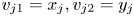
Let  $\theta =0.1$, 0.2, 0.5, 1, 2, Figure 4(a) and (b) shows that all
  ${u K'_q(u)}/{K_q(u)}$ are nonpositive and decreasing in
  $u\in (0,1)$, and all
  ${u L'_{\beta _{4}}(u)}/{L_{\beta _{4}}(u)}$ are positive and decreasing in
  $u\in (0,1)$. Figure 4(c) and (d) shows that all
  ${\beta _4}(u)\leq u{\beta '_4}(u)$ and
  $1-q(u)\geq (1-u)q'(u),$ for all
  $u\in (0,1)$. Figure 5 shows that all
  ${f_{\rm ARCL}}/{f_{\rm ARSL}}$ are increasing in
  $u\in (0,1)$. And thus,
  $\tau _{\rm ARCL}\prec _c \tau _{\rm ARSL}$ and
  $\tau _{\rm ARCL}\geq _{\textrm {lr}} \tau _{\rm ARSL}$ hold.

Figure 4. (a) Plots of the function  ${u K'_q(1-u)}/{K_q(1-u)}$, (b) plots of the function
  ${u L'_{\beta _{m+1}}(u)}/{L_{\beta _{m+1}}(u)}$, (c) plots of the function
 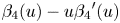 ${\beta _4}(u)-u{\beta _4}'(u)$ and (d) plots of the function
 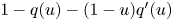 $1-q(u)-(1-u)q'(u)$.

Figure 5. Plots of the function 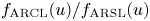 $f_{\rm ARCL}(u)/f_{\rm ARSL}(u)$.
Under the setup of Example 3, taking  $\theta =1.6$. Figure 6(a) and (b) illustrates that neither
  $\tau _{\rm ARCL}\succ _b \tau _{\rm ARSL}$ nor
  $\tau _{\rm ARCL}\geq _{\textrm {lr}} \tau _{\rm ARSL}$ holds. The following Theorem 5 gives the likelihood ordering and aging faster ordering in terms of the reversed hazard rate between the component and system levels under the framework of complete matching redundancies.
Theorem 5 If
(1)
${(1-u) K'_{\beta _{m+1}}(u)}/{K_{\beta _{m+1}}(u)}$ is nonpostive decreasing in $u\in (0,1)$,(2)
${(1-u) L'_q(1-u)}/{L_q(1-u)}$ is nonnegative increasing in $u\in (0,1)$ and(3)
$q(1-u)\leq \min \{1-u, (1-u)q'(1-u)\}$, for all $u\in (0,1)$,


Figure 6. For  $\theta =1.6,$ (a) plot of the function
 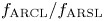 $f_{\rm ARCL}/f_{\rm ARSL}$ and (b) plot of the function
  ${h}_{\rm ARCL}/{h}_{\rm ARSL}$.
then
 $$\tau_{\rm ARCL}\succ _b \tau_{\rm ARSL},$$
and
 $$\tau_{\rm ARCL}\geq_{\textrm{lr}} \tau_{\rm ARSL}.$$


3.3. Nonmatching case
For the coherent system with  ${\textrm {d.i.d.}}$ components and spares, suppose that spares and original components are independent, in the nonmatching case, under conditions
  ${((1-p)q'(p))}/{(1-q(p))}$ is increasing in
  $p\in (0,1),$ Zhang et al. [Reference Zhang, Amini-Seresht and Ding50] proved that
 \begin{equation} \tau_{\rm ARCL}\geq_{\textrm{rh}} \tau_{\rm ARSL}. \end{equation}
The following theorem generalizes Eq. (17) to the coherent systems with dependence of spares and original components in the case of the reversed hazard rate ordering. It incorporates or generalizes many known results in the literature. For more details, refer to Theorem 3.2 of Gupta and Nanda [Reference Gupta and Nanda15], Theorem 3.1 of Misra et al. [Reference Misra, Dhariyal and Nitin30], Theorem 3 of Gupta and Kumar [Reference Gupta and Kumar14] and Theorem 3.4 of Zhang et al. [Reference Zhang, Amini-Seresht and Ding50]. For convenience, denote
 $$\alpha_{j}^{C}(v_1,v_2,\ldots,v_{m+1})=\frac{v_{j}\partial C(v_1,v_2,\ldots,v_{m+1})/\partial v_j}{C(v_1,v_2,\ldots,v_{m+1})},\quad j=1,2,\ldots,m+1$$
Theorem 6 If
(1)
$\alpha _{j}^{C}(v_1,v_2,\ldots ,v_{m+1})$ is decreasing in $v_j\in (0,1)$, for all $j=1,2,\ldots ,m+1,$(2)
$L_q(1-u)$ is decreasing in $u\in (0,1)$ and(3)
$q(1-u)\leq 1-u$ for all $u\in (0,1)$,


then
 $$\tau_{\rm ARCL}\geq_{\textrm{rh}} \tau_{\rm ARSL}.$$
One natural question arises that whether the hazard rate ordering, aging faster ordering in terms of the reversed hazard rate and the hazard rate hold between  $\tau _{\rm ARCL}$ and
  $\tau _{\rm ARSL}$ for the nonmatching case. Unfortunately, Counterexample 1 gives a negative answer even for the independent case.
Counterexample 1 For a coherent systems  $T=\wedge \{X_1,X_2\}$ with i.i.d. components
  $X_1$ and
  $X_2$ having exponential lifetimes with parameters
  $\lambda =2$. Let
  $Y_1$ and
  $Y_2$ be lifetimes of two i.i.d. spares having exponential lifetimes with parameters
  $\lambda =1$. We have
 $$F_{\rm ARCL}(1-e^{- x},1-e^{{-}2 x})=1-(1-(1-e^{{-}2 x}) (1-e^{{-}x}))^{2}$$
and
 $$F_{\rm ARSL}(1-e^{- x},1-e^{{-}2 x})=(1-e^{{-}4 x}) (1-e^{{-}2 x}).$$
And it holds that
 \begin{align*} {\tilde{h}_{\rm ARCL}(1-e^{- x},1-e^{{-}2 x})}& =\frac{2 (e^{x}+3) (e^{x}+e^{2 x}-1)}{1-e^{x}-2 e^{2 x}+e^{4 x}+e^{5 x}},\\ {{h}_{\rm ARCL}(1-e^{- x},1-e^{{-}2 x})}& =\frac{2 (e^{{-}x} (1-e^{{-}2 x})+2 e^{{-}2 x} (1-e^{{-}x}))}{1-(1-e^{{-}2 x}) (1-e^{{-}x})},\\ {\tilde{h}_{\rm ARSL}(1-e^{- x},1-e^{{-}2 x})}& =\frac{2 (e^{2 x}+3)}{e^{4 x}-1},\\ {{h}_{\rm ARSL}(1-e^{- x},1-e^{{-}2 x})}& =\frac{2 e^{{-}2 x} (1-e^{{-}4 x})+4 e^{{-}4 x} (1-e^{{-}2 x})}{1-(1-e^{{-}4 x}) (1-e^{{-}2 x})}. \end{align*}
From Figure 7(a), (b) and (c), it obviously can be seen that  ${\tilde {h}_{\rm ARCL}}/{\tilde {h}_{\rm ARSL}}$,
  ${\bar F_{\rm ARCL}}/{\bar F_{\rm ARSL}}$ and
  ${{h}_{\rm ARCL}}/{{h}_{\rm ARSL}}$ are all not monotone on
  $(0,\infty ),$ which mean
  $\tau _{\rm ARCL}\succ _b \tau _{\rm ARSL}$,
  $\tau _{\rm ARCL}\succ _c \tau _{\rm ARSL}$ and
  $\tau _{\rm ARCL}\geq _{\textrm {hr}} \tau _{\rm ARSL}$ are all invalid.

Figure 7. (a) Plot of the function  $\tilde {h}_{\rm ARCL}/\tilde {h}_{\rm ARSL}$, (b) plot of the function
  $\bar F_{\rm ARCL}/\bar F_{\rm ARSL}$ and (c) plot of the function
  ${h}_{\rm ARCL}/{h}_{\rm ARSL}$.
4. Application
From a practical point of view, modern systems, such as the new energy vehicles industry, respond to the requirements of safe and stable operation; it is hoped that the probability of the running interruption of the core components can be reduced. A possible component level versus system level at active redundancies for coherent systems with dependent components application scenarios are provided below for practical use and reference for future research.
As the power source and energy carrier of new energy vehicles, power battery is a key component. However, the backwardness of power battery-related technologies seriously restricts the development of electric vehicles, which are mainly manifested in poor endurance, short service life and unstable safety. In pure electric vehicles and grid energy storage applications, single batteries are connected in series to meet voltage requirements and in parallel to meet capacity requirements. Series and parallel connections often exist simultaneously. Among them, the battery used in the Beijing Olympic Games and the Shanghai World Expo for pure electric buses adopts a parallel-series connection, and the grid battery energy storage often adopts a series-parallel connection. Therefore, the battery formation mode is an extremely active research field in the lithium-ion battery management system, and the quality of its evaluation method largely determines the overall performance of the battery management system. As shown in Figure 8(a) and (b), we will explore the performance of the series-parallel battery group and the parallel-series battery group. To solve the above problems, we give the following assumptions:
(1) Suppose we have 12 batteries
$B_{11},B_{12},B_{13},B_{14},B_{21},B_{22},B_{23},B_{24},B_{31},B_{32},B_{33},B_{34},$ which are made in the same batch and the same manufacturer.(2) It is assumed that the failure data of a single battery has been obtained through the durability test, and the lifetime distribution of battery can be estimated from the failure data, let us assume a Weibull distribution;
(3) Considering the influence of the environment and stress level of the battery group, it is assumed that the batteries that make up the battery group are interdependent, and the dependency is described by copula.
(4) According to Section 3.1, suppose that
and$$C'(v_1,v_2,v_3,v_4)=\left(\prod_{1=1}^{4}v_i\right)e^{-\theta_1\prod_{1=1}^{4}\log v_i}, \quad v_i\in[0,1]$$
$$C(v_1,v_2,v_3)=\prod_{i=1}^{3}v_i+\theta_2\prod_{i=1}^{3}v_i(1-v_i),\quad v_i\in[0,1].$$


Figure 8. (a) Series-parallel battery group and (b) parallel-series battery group.
Next, we will use the work of this article to explore how to optimize the battery group method from a theoretical point of view to improve the life of the power battery group. From Example 2, we find the performance of the parallel-series battery group is better than the series-parallel battery group. Therefore, to improve the reliability of the battery group, the battery formation mode is the parallel-series group. The research results provide some theoretical support for engineers to design more complex power battery groups. However the series-parallel battery group is conducive to the detection and management of the individual cells of the system.
5. Conclusion
This paper investigates the case that the vector of the spare lifetimes and the vector of the original component lifetimes are dependent. In this framework, we consider the issue of stochastic comparison of multi-active complete matching and nonmatching spares redundancies at the component level versus the system level, respectively. In cases of the nonmatching and matching spares, we got the sufficient conditions that are presented to compare component and system redundancies by means of the hazard rate ordering and the reversed hazard rate ordering, and we also obtain the result for relative aging ordering. Our work extend the works of Zhang et al. [Reference Zhang, Amini-Seresht and Ding50] and Hazra and Misra [Reference Hazra and Misra16] and complements existing literature. However, for the general case, that is, consider the assumption of all components are d.n.i.d., which is an important question in future study, and Yan et al. [Reference Yan, Zhang and Zhao46] stochastically compares allocations of standby redundancies in series systems with exponential components at the component level versus the system level in sense of the likelihood ratio ordering, that is,
 \begin{equation} \wedge(X_1+Y_1,X_2+Y_2)\geq_{\textrm{lr}}[{\wedge}(X_1,X_2)]+[{\wedge}(Y_1,Y_2)]. \end{equation}
Based on Eq. (18), it is also of great interest to consider the corresponding conclusion when replacing active redundancy in this article as standby redundancy, where Eqs. (4) and (5) are replaced as
 \begin{align*} \tau_{\rm ARCL}& =\tau(X_1+ Y_{11}+ \cdots+{Y}_{m1}, X_2+ Y_{12}+ \cdots+{Y}_{m2}, \ldots,X_n+ Y_{1n}+\cdots+{Y}_{mn}),\\ \tau_{\rm ARSL}& =\tau(X_1, X_2, \ldots, X_n)+\tau(Y_{11},Y_{12},\ldots,Y_{1n})+\cdots+ \tau(Y_{m1},Y_{m2},\ldots,Y_{mn}) , \end{align*}
respectively, which remains as an open problem. On the other hand, in design and analysis of the redundancy allocation issue, engineer must have some components or subsystems in the inventory to replace the failed part. The number of components in inventory may be limited by factors such as budget or storage space. Therefore, the redundancy allocation problem is to find a way to maximize reliability while reducing costs. For example, Hsieh [Reference Hsieh18] discusses the combination of cold standby strategy and component mixing and proposes hybrid strategy to optimize reliability redundancy allocation problem. Thus, in the follow-up, we have to consider not only the optimization of the allocation should be considered but also the minimization of the cost.
Acknowledgments
This work is supported by the National Natural Science Foundation of China (11861058). The authors are indebted to editor and anonymous referees, for insightful comments and help suggestions, which have greatly improved the presentation of this manuscript and for bringing our attention to recent publications in the relevant literature.
Competing interest
The authors declare no conflict of interest.
Appendix. Proof of all main results
Proof of Theorem 1
It is obvious that  $\bar F_{\rm ARCL}(u)-\bar F_{\rm ARSL}(u)\geq 0$, which is equivalent to
 $$q(1-\beta_{m+1}(u))+\beta_{m+1}(1-q(1-u))\geq 1.$$
The proof is completed.
Proof of Theorem 2
According to Definition 1  $({\rm ii})$, the desired result is equivalent to
 $$\Lambda(u)=\displaystyle\frac{\bar F_{\rm ARCL}(u)}{\bar F_{\rm ARSL}(u)}=\frac{q(1-{\beta_{m+1}}(u))}{1-{\beta_{m+1}}(1-q(1-u))}$$
is increasing in  $u\in (0,1)$. Observe that
 \begin{align*} \frac{\partial\Lambda(u)}{\partial u} & \overset{\rm sgn}{=}\frac{q'(1-u){\beta'_{m+1}}(1-q(1-u))}{1-{\beta_{m+1}}(1-q(1-u))} -\frac{{\beta'_{m+1}}(u)q'(1-{\beta_{m+1}}(u))}{q(1-{\beta_{m+1}}(u))}\\ & \overset{\rm sgn}{=}\frac{q(1-u){\beta'_{m+1}}(1-q(1-u))}{1-{\beta_{m+1}}(1-q(1-u))}\cdot \frac{(1-u)q'(1-u)}{q(1-u)}-\frac{(1-u){\beta'_{m+1}}(u)}{1-{\beta_{m+1}}(u)}\\ & \quad \cdot\frac{(1-{\beta_{m+1}}(u))q'(1-{\beta_{m+1}}(u))}{q(1-{\beta_{m+1}}(u))}\\ & \geq \frac{(1-u){\beta'_{m+1}}(u)}{1-{\beta_{m+1}}(u)}\left[\frac{(1-u)q'(1-u)}{q(1-u)} -\frac{(1-{\beta_{m+1}}(u))q'(1-{\beta_{m+1}}(u))}{q(1-{\beta_{m+1}}(u))}\right]\\ & =L_{\beta_{m+1}}(u)[K_q(1-u)-K_q(1-{\beta_{m+1}}(u))]\\ & \geq 0, \end{align*}
note that  ${\beta _{m+1}}(x)$ and
  $q(x)$ are increasing in
  $x\in [0,1]$, and thus,
  $L_{\beta _{m+1}}(x)$ and
  $K_q(x)$ are nonnegative for all
  $x\in [0,1],$ then, the first inequality is derived from conditions (1) and (2), and the second inequality comes from conditions (1), (2) and (3), which completes the proof.
Proof the nonnegative and increasing property of $L_{\beta _{3}}(u)$ in (12)

Obvious that
 \begin{align*} L_{\beta_{3}}(u)& =\frac{(1-u){\beta'_3}(u)}{1-{\beta_3}(u)}\\ & \overset{\rm sgn}{=}3 u^{2} (\theta_2 (1-2 u) (1-u)^{2}+1)\\ & \overset{\rm sgn}{=}1+\theta_2 (1-2 u) (1-u)^{2}=:\mu(u;\theta_2). \end{align*}
In the following, we prove the nonnegative of  $\mu (u;\theta )$.
Case 1: 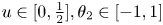 $u\in [0,\frac {1}{2}],\theta _2\in [-1,1]$. It is easy to see that
 $$0\leq(1-2u)(1-u)^{2}\leq 1,$$
for any  $\theta _2\in [-1,1],$ we then have
 $$\mu(u;\theta_2)\geq \mu(u;-1)=1-(1-2u)(1-u)^{2}\geq 0$$
Case 2: for 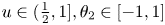 $u\in (\frac {1}{2},1],\theta _2\in [-1,1]$. Note that
 $${-}1<(1-2u)(1-u)^{2}\leq 0,$$
for any  $\theta _2\in [-1,1],$ we have
 $$\mu(u;\theta_2)\geq \mu(u;1)=1+(1-2u)(1-u)^{2}\geq 0 .$$
It suffices to prove  $L_{\beta _{3}}(u)$ is increasing in
  $u\in [0,1]$. After some simplifications, we have
 $$\eta(u;\theta_2):={L'_{\beta_{3}}}(u)\overset{\rm sgn}{=}a(u)\theta_2 ^{2}+b(u)\theta_2 +c(u),$$
where
 \begin{align*} a(u)& = u^{3}(1-u)^{4}\geq 0,\\ b(u)& =({-}3 u^{5}-2 u^{4}+2 u^{3}+12 u^{2}-11 u+2),\\ c(u)& =u+2\geq 0. \end{align*}
Obvious that, taking  $u=0$ and
  $u=1$, then
  $\eta (u;\theta _2)=2\theta _2+2$ and
  $\eta (u;\theta _2)=2$, respectively, and thus
  $\eta (u;\theta _2)\geq 0$. For any
  $u\in (0,1,)$ from the properties of quadratic function, if
  $-b(u)/(2a(u))\geq 0,$ then
 $$\eta(u;1)\geq 0\Longrightarrow \eta(u;\theta_2)\geq 0$$
Similarly, if  $-b(u)/(2a(u))\leq 0,$ then
 $$\eta(u;-1)\geq 0\Longrightarrow \eta(u;\theta_2)\geq 0$$
Figure A.1 shows that  $\eta (u;1)\geq 0$ and
  $\eta (u;-1)\geq 0$.

Figure A.1. Plots of the function  $\eta (u;-1)$ and
  $\eta (u;1)$.
To sum up, for any  $u\in [0,1]$ and
  $\theta _2\in [-1,1],$ we have showed that
  $L_{\beta _{3}}(u)$ is nonnegative and increasing in
  $u$.
$u$.
Proof of Theorem 4
We have two cases to prove this theorem.
Case 1:  $\tau _{\rm ARCL}\prec _c \tau _{\rm ARSL}$. Denote
  ${{h}_{\rm ARCL}({u})}$ and
  ${{h}_{\rm ARSL}({u})}$ the hazard rate of
  $\tau _{\rm ARCL}$ and
  $\tau _{\rm ARSL},$ respectively, then
 \begin{align*} {{h}_{\rm ARCL}({u})}& =\frac{{\beta'_{m+1}}({u})q'(1-{\beta_{m+1}}({u}))}{q(1-{\beta_{m+1}}({u}))},\\ {{h}_{\rm ARSL}({u})}& =\frac{q'(1-u){\beta'_{m+1}}({1-q(1-u)})}{1-{\beta_{m+1}}({1-q(1-u)})}. \end{align*}
According to Definition 2  $({\rm i})$, the desired result is equivalent to
  ${{h}_{\rm ARCL}({u})}/{{h}_{\rm ARSL}({u})}$ is increasing in
  $u_i,\;i=1,2,\ldots ,m+1$. Obverse that,
 \begin{align*} \frac{{{h}_{\rm ARCL}({u})}}{{{h}_{\rm ARSL}({u})}}& =\frac{ {\beta'_{m+1}}({u})q'(1-{\beta_{m+1}}({u}))}{q(1-{\beta_{m+1}}({u}))}\cdot \frac{1-{\beta_{m+1}}({1-q(1-u)})}{q'(1-u){\beta'_{m+1}}({1-q(1-u)})}\\ & =\frac{(1-u){\beta'_{m+1}}({u})}{1-{\beta_{m+1}}({u})}\cdot\frac{(1-{\beta_{m+1}}({u})) q'(1-{\beta_{m+1}}({u}))}{q(1-{\beta_{m+1}}({u}))}\cdot \frac{q(1-u)}{(1-u)q'(1-u)}\\ & \quad \times\frac{1-{\beta_{m+1}}({1-q(1-u)})}{q(1-u){\beta'_{m+1}}({1-q(1-u)})}\\ & =\frac{L_{\beta_{m+1}}(u)}{L_{\beta_{m+1}}(1-q(1-u))}\cdot\frac{K_q(1-{\beta_{m+1}}(u))}{K_q(1-u)}. \end{align*}
Note that  ${\beta _{m+1}}(u)$ is increasing in
  $u\in [0,1],$ which implies
  $L_{\beta _{m+1}}(u)$ is nonnegative for all
  $u\in [0,1],$ and
  $q(1-u)$ are increasing in
  $(1-u)\in [0,1]$, which implies
  $K_q(1-u)$ is nonnegative for all
  $(1-u)\in [0,1],$ we then have
 $$\left[\frac{L_{\beta_{m+1}}(u)}{L_{\beta_{m+1}}(1-q(1-u))}\right]'\geq 0\ \text{and}\ \left[\frac{K_q(1-{\beta_{m+1}}(u))}{K_q(1-u)}\right]'\geq 0 \ \text{imply}\ \left[\frac {{h}_{\rm ARCL}({u})}{{h}_{\rm ARSL}({u})}\right]'\geq 0,$$
and
 $$\left[\frac{L_{\beta_{m+1}}(u)}{L_{\beta_{m+1}}(1-q(1-u))}\right]'\overset{\rm sgn}{=} \frac{L'_{\beta_{m+1}}(u)}{L_{\beta_{m+1}}(u)}- \frac{q'(1-u)L'_{\beta_{m+1}}(1-q(1-u))}{L_{\beta_{m+1}}(1-q(1-u))}.$$
From the assumption that  ${uL'_{\beta _{m+1}}(u)}/{L_{\beta _{m+1}}(u)}$ is positive and decreasing in
  $u\in (0,1)$ and
  $1-q(1-u)\geq uq'(1-u),$ and
  $q(1-u)\leq 1-u,$ for all
  $u\in (0,1),$ it follows that
 \begin{equation} \frac{uL'_{\beta_{m+1}}(u)}{L_{\beta_{m+1}}(u)}\geq \frac{(1-q(1-u))L'_{\beta_{m+1}}(1-q(1-u))}{L_{\beta_{m+1}}(1-q(1-u))}\geq \frac{uh'(1-u)L'_{\beta_{m+1}}(1-q(1-u))}{L_{\beta_{m+1}}(1-q(1-u))}. \end{equation}
Similarity,
 $$\left[\frac{K_q(1-{\beta_{m+1}}(u))}{K_q(1-u)}\right]'\overset{\rm sgn}{=}\frac{K'_q(1-u)}{K_q(1-u)}-\frac{{\beta'_{m+1}}(u)K'_q(1-{\beta_{m+1}}(u))}{K_q(1-{\beta_{m+1}}(u))}.$$
From the assumption that  ${u K'_q(1-u)}/{K_q(1-u)}$ is nonpositive and increasing in
  $u\in (0,1)$ and based on Lemma 1, it is obvious that
  ${\beta _{m+1}}(u)\leq \min \{u, u{\beta '_{m+1}}(u)\}$, for all
  $u\in (0,1),$ we have
 \begin{equation} \frac{uK'_q(1-u)}{K_q(1-u)}\geq \frac{{\beta_{m+1}}(u)K'_q(1-{\beta_{m+1}}(u))}{K_q(1-{\beta_{m+1}}(u))} \geq\frac{u{\beta'_{m+1}}(u)K'_q(1-{\beta_{m+1}}(u))}{K_q(1-{\beta_{m+1}}(u))}. \end{equation}
 $$\left[\frac{L_{\beta_{m+1}}(u)}{L_{\beta_{m+1}}(1-q(1-u))}\right]'\geq 0,\quad \left[\frac{K_q(1-{\beta_{m+1}}(u))}{K_q(1-u)}\right]'\geq 0$$
And thus  $\tau _{\rm ARCL}\prec _c \tau _{\rm ARSL}$.
Case 2:  $\tau _{\rm ARCL}\geq _{\textrm {lr}} \tau _{\rm ARSL}$. Based on Theorem 2, we have
  ${uK'_q(1-u)}/{K_q(1-u)}$ is nonpositive and increasing in
  $u\in (0,1)$ implies
  $K_q(1-u)$ is decreasing in
  $(1-u)\in (0,1)$, and
  ${u L'_{\beta _{m+1}}(u)}/{L_{\beta _{m+1}}(u)}$ is positive and decreasing in
  $u\in (0,1)$ implies
  $L_{\beta _{m+1}}(u)$ is increasing in
  $u\in (0,1)$. According to Theorem 1.C.4 in Shaked and Shantikumar [Reference Shaked and Shantikumar40], it is well know that
  $X\geq _{\textrm {lr}}Y$. Therefore, if conditions (1), (2) and (3) hold, we also have
  $\tau _{\rm ARCL}\geq _{\textrm {lr}} \tau _{\rm ARSL}$. Thatcompletes the proof.
Proof of Theorem 5
We have two cases to prove this theorem.
Case 1:  $\tau _{\rm ARCL}\succ _b \tau _{\rm ARSL}$. Denote
  ${\tilde {h}_{\rm ARCL}({u})}$ and
  ${\tilde {h}_{\rm ARSL}({u})}$ the reversed hazard rate of
  $\tau _{\rm ARCL}$ and
  $\tau _{\rm ARSL},$ respectively, then
 \begin{eqnarray*} {\tilde{h}_{\rm ARCL}({u})} & =\frac{ {\beta'_{m+1}}({u})q'(1-{\beta_{m+1}}({u}))}{1-q(1-{\beta_{m+1}}({u}))},\\ {\tilde{h}_{\rm ARSL}({u})}& =\frac{q'(1-u){\beta'_{m+1}}({1-q(1-u)})}{{\beta_{m+1}}({1-q(1-u)})}. \end{eqnarray*}
According to Definition 2(ii), the desired result is equivalent to  ${\tilde {h}_{\rm ARCL}({u})}/{\tilde {h}_{\rm ARSL}({u})}$ is increasing in
  $u,$ we have
 \begin{align*} \frac{{\tilde{h}_{\rm ARCL}({u})}}{{\tilde{h}_{\rm ARSL}({u})}}& =\frac{ {\beta'_{m+1}}({u})q'(1-{\beta_{m+1}}({u}))}{1-q(1-{\beta_{m+1}}({u}))}\cdot \frac{{\beta_{m+1}}({1-q(1-u)})}{q'(1-u){\beta'_{m+1}}({1-q(1-u)})}\\ & =\frac{u{\beta'_{m+1}}({u})}{{\beta_{m+1}}({u})}\cdot\frac{{\beta_{m+1}}({u}) q'(1-{\beta_{m+1}}({u}))}{1-q(1-{\beta_{m+1}}({u}))}\\ & \quad \cdot \frac{1-q(1-u)}{uh'(1-u)}\cdot \frac{{\beta_{m+1}}({1-q(1-u)})}{(1-q(1-u)){\beta'_{m+1}}({1-q(1-u)})}\\ & =\frac{K_{\beta_{m+1}}(u)}{K_{\beta_{m+1}}(1-q(1-u))}\cdot\frac{L_q(1-{\beta_{m+1}}(u))}{L_q(1-u)}. \end{align*}
Note that  ${\beta _{m+1}}(u)$ is increasing in
  $u\in [0,1],$ which implies
  $K_{\beta _{m+1}}(u)$ is nonnegative for all
  $u\in [0,1],$ and
  $q(1-u)$ are increasing in
  $(1-u)\in [0,1]$, which implies
  $L_q(1-u)$ is nonnegative for all
  $(1-u)\in [0,1],$ we then have
 $$\left[\frac{K_{\beta_{m+1}}(u)}{K_{\beta_{m+1}}(1-q(1-u))}\right]'\geq 0 \ \text{and}\ \left[\frac{L_q(1-{\beta_{m+1}}(u))}{L_q(1-u)}\right]'\geq 0 \ \text{imply}\ \left[\frac {\tilde{h}_{\rm ARCL}({u})}{\tilde{h}_{\rm ARSL}({u})}\right]'\geq 0$$
and
 $$\left[\frac{K_{\beta_{m+1}}(u)}{K_{\beta_{m+1}}(1-q(1-u))}\right]'\overset{\rm sgn}{=} \frac{K'_{\beta_{m+1}}(u)}{K_{\beta_{m+1}}(u)}- \frac{q'(1-u)K'_{\beta_{m+1}}(1-q(1-u))}{K_{\beta_{m+1}}(1-q(1-u))}.$$
From the assumption that  ${(1-u) K'_{\beta _{m+1}}(u)}/{K_{\beta _{m+1}}(u)}$ is nonpositive and decreasing in
  $u\in (0,1)$ and
  $q(1-u)\leq \min \{1-u,(1-u)q'(1-u)\},$ for all
  $u\in (0,1),$ we have
 \begin{equation} \frac{(1-u)K'_{\beta_{m+1}}(u)}{K_{\beta_{m+1}}(u)}\geq \frac{q(1-u)K'_{\beta_{m+1}}(1-q(1-u))}{K_{\beta_{m+1}}(1-q(1-u))}\geq \frac{(1-u)q'(1-u)K'_{\beta_{m+1}}(1-q(1-u))}{K_{\beta_{m+1}}(1-q(1-u))}. \end{equation}
Similarity,
 $$\left[\frac{L_q(1-{\beta_{m+1}}(u))}{L_q(1-u)}\right]'\overset{\rm sgn}{=} \frac{L'_q(1-u)}{L_q(1-u)}-\frac{{\beta'_{m+1}}(u)L'_q(1-{\beta_{m+1}}(u))}{L_q(1-{\beta_{m+1}}(u))}.$$
From the assumption that  ${(1-u) L'_q(1-u)}/{L_q(1-u)}$ is positive and increasing in
  $u\in (0,1)$ and according to Lemma 1, we have
  $1-{\beta _{m+1}}(u)\geq (1-u){\beta '_{m+1}}(u),$ and
  ${\beta _{m+1}}(u)\leq u,$ hold, for all
  $u\in (0,1),$ thus
 \begin{equation} \frac{(1-u)L'_q(1-u)}{L_q(1-u)}\geq \frac{(1-{\beta_{m+1}}(u))L'_q(1-{\beta_{m+1}}(u))}{L_q(1-{\beta_{m+1}}(u))}\geq \frac{(1-u){\beta'_{m+1}}(u)L'_q(1-{\beta_{m+1}}(u))}{L_q(1-{\beta_{m+1}}(u))}. \end{equation}
 $$\left[\frac{K_{\beta_{m+1}}(u)}{K_{\beta_{m+1}}(1-q(1-u))}\right]'\geq 0,\quad \left[\frac{L_q(1-{\beta_{m+1}}(u))}{L_q(1-u)}\right]'\geq 0.$$
And thus  $\tau _{\rm ARCL}\succ _b \tau _{\rm ARSL}$.
Case 2:  $\tau _{\rm ARCL}\geq _{\textrm {lr}} \tau _{\rm ARSL}$. According to Theorem 3, we have
  ${(1-t) K'_{\beta _{m+1}}(u)}/{K_{\beta _{m+1}}(u)}$ is nonpositive decreasing in
  $u\in (0,1)$ implies
  $K_{\beta _{m+1}}(u)$ is decreasing in
  $u\in (0,1)$, and
  ${x L'_q(x)}/{L_q(x)}$ is nonnegative decreasing in
  $x\in (0,1)$ implies
  $L_q(x)$ is increasing in
  $x\in (0,1),$ where
  $x=1-u$. According to Theorem 1.C.4 in Shaked and Shantikumar [Reference Shaked and Shantikumar40], it is well know that
  $X\geq _{\textrm {lr}}Y$. Therefore, if conditions (1), (2) and (3) hold, we also have
  $\tau _{\rm ARCL}\geq _{\textrm {lr}} \tau _{\rm ARSL}$. That completes the proof.
Proof of Theorem 6
According to Definition 1(i), the desired result is equivalent to
 $$\Lambda(u_1,u_2,\ldots,u_{m+1})= \frac{F_{\rm ARCL}(u_1,u_2,\ldots,u_{m+1})}{F_{\rm ARSL}(u_1,u_2,\ldots,u_{m+1})} =\frac{1-q(1-C(u_1,u_2,\ldots,u_{m+1}))}{C(1-q(1-u_1),1-q(1-u_2),\ldots,1-q(1-u_{m+1}))}$$
is increasing in  $u_i\in (0,1),\ i=1,2,\ldots ,m+1$. Observe that
 \begin{align*} \frac{\partial\Lambda(u_1,u_2,\ldots,u_{m+1})}{\partial u_i}& \overset{\rm sgn}{=} \frac{q'(1-C(\mathbf{u})) \partial C(\mathbf{u})/\partial u_i}{1-q(1-C(\mathbf{u})}-\frac{q'(1-u_i) \partial C(\mathbf{1-q(1-u)})/\partial (1-q(1-u_i))}{C(\mathbf{1-q(1-u)})}\\ & \overset{\rm sgn}{=} \alpha_{i}^{C}(\mathbf{u})\cdot L_q(1-C(\mathbf{u}))-\alpha_{i}^{C}(\mathbf{1-q(1-u)})\cdot L_q(1-u_i)\\ & \geq 0, \end{align*}
where  $\mathbf {u}=\{u_1,u_2,\ldots ,u_{m+1}\}$,
  ${C}(\mathbf {u})=C(u_1,u_2,\ldots ,u_{m+1}),$
  $\mathbf {1-q(1-u)}=\{1-q(1-u_1), 1-q(1-u_2),\ldots , 1-q(1-u_{m+1})\}$. The inequality is derived from conditions (1), (2) and (3) based on
  $1-q(1-u_i)\geq {u_i}$ and
  $C(\mathbf {u})\leq u_i,\ i=1,2,\ldots ,m+1$, which completes the proof.


