1. INTRODUCTION
Polar navigation technology has been a widely researched navigation field with the development of worldwide transportation (Yao et al., Reference Yao, Xu, Li, Sun and Tong2016; Li et al., Reference Li, Ben, Yu and Tan2016; Reference Li, Ben and Yu2015; Reference Li, Ben, Sun and Huo2014a; Reference Li, Sun, Ben and Yu2014b; Pedersen, Reference Pedersen1960). Due to its special geographical characteristics, general navigation methods such as satellite navigation, radio navigation and geomagnetic navigation do not always work efficiently in polar regions (Tang et al., Reference Tang, Wu and Wu2009; Naumann, Reference Naumann2011; Zhao, Reference Zhao2017). Inertial navigation is not affected by external conditions such as polar geomagnetic changes and solar storms. With consideration of the self-contained merits, a Strapdown Inertial Navigation System (SINS) is the most preferred system for a vehicle in polar regions (Pedersen, Reference Pedersen1960). As the geographical meridians converge rapidly in the polar regions, traditional inertial navigation methods fail in these areas. All mechanisms in SINS using traditional latitude and longitude as the position parameterisations fail to provide accurate positions and orientations in such cases. If the local geographic navigation frame is chosen as the navigation frame, the turn rate of the navigation frame will be involved in terms of a tangent function. A potential problem will arise when the vehicle travels close to the Earth's poles. This is because when the latitude angle φ approaches ±90°, tan φ will be infinite (Bekir, Reference Bekir2007). The wander azimuth mechanism is one option to circumvent the polar navigation problem. The corresponding idea is to prevent the navigation frame from rotating about the z-axis. However, for the wander azimuth mechanism, it is impossible to distinguish between the wander azimuth angle and the longitude. This implies that the wander azimuth angle may not be the answer to navigation near the poles (Bekir, Reference Bekir2007). Navigation in an Earth-Centred Earth-Fixed (ECEF) frame is another choice for polar navigation. However, the ECEF mechanism inherits some limitations due to its non-horizontal characteristic. More specifically, the diverging vertical errors will be coupled into an ECEF-based system, affecting the accuracy of the position in other directions. In this respect, it is not suitable for long range and long endurance missions (Titterton and Weston, Reference Titterton and Weston2014).
To address the problems of polar navigation, a transversal coordinate system and corresponding navigation mechanism was proposed in Broxmeyer (Reference Broxmeyer1964) and Lyon (Reference Lyon1984). In this navigation mechanism, the traditional geographic coordinate system is transversely rotated, which makes the original north and south poles change to the equator of the transversal coordinate system. The traditional transversal navigation uses a spherical model for the earth, which brings advantages of brevity and convenience for transverse rotation of the geographic coordinate system. Unfortunately, the Earth is an ellipsoid and the corresponding simplification consequentially introduces principle errors for an Inertial Navigation System (INS). Some interesting research work, such as transformation of navigation parameters and reset and damping of transversal SINS, has been completed based on transversal mechanisation (Li et al., Reference Li, Ben and Yu2015; Reference Li, Ben, Sun and Huo2014a; Reference Li, Sun, Ben and Yu2014b; Watland and Ariz, Reference Watland and Ariz1995).
In Li et al. (Reference Li, Ben, Sun and Huo2014a; Reference Li, Sun, Ben and Yu2014b), performances and error characteristics of transversal navigation based on the sphere model were theoretically analysed. The principle errors caused by the spherical model are mainly in the form of oscillation errors, and damping technology, widely applied in traditional SINS, is used to suppress those oscillation errors (Li et al., Reference Li, Ben and Yu2015; Reference Li, Ben, Sun and Huo2014a; Reference Li, Sun, Ben and Yu2014b). However, constant errors from velocities remain. Due to these principle errors, transversal navigation using the sphere model is not acceptable for a high-precision INS. In order to further improve the navigation precision, many researchers have addressed these principle errors. In Yao et al. (Reference Yao, Xu, Li, Sun and Tong2016) and Li et al. (Reference Li, Ben, Yu and Tan2016) the ellipsoidal Earth model is used to address the theoretical error resulting from the inaccurate spherical Earth model. In Yao et al. (Reference Yao, Xu, Li, Sun and Tong2016), implicit equations of radii using a transversal ellipsoidal Earth model are derived in detail. To obtain analytic solutions for these radii, an additional angle parameter is introduced, which unfortunately cannot be obtained analytically in the differential equation. It should be noted that Equation (15) of Yao et al. (Reference Yao, Xu, Li, Sun and Tong2016) has been approximated and simplified. In Li et al. (Reference Li, Ben, Yu and Tan2016), the radius of the transversal meridian and the radius of the transversal prime vertical are derived. Since in a transversal coordinate system, “latitude” or “longitude” is affected by both “north” velocity and “east” velocity, the individual radius of the transversal meridian or the radius of the transversal prime vertical are not so suitable for coupling of transversal navigation. In addition, the height in transversal navigation is omitted in Li et al. (Reference Li, Ben, Yu and Tan2016).
Inspired by the ideas of Yao et al. (Reference Yao, Xu, Li, Sun and Tong2016) and Li et al. (Reference Li, Ben, Yu and Tan2016), a more rigorous transversal navigation mechanism is proposed in this paper. Starting from the relationship between Euclidean coordinates and spherical coordinates, the main equations of transversal polar navigation based on an ellipsoidal Earth model are derived in detail, including attitude, velocity and position differential equations. The main contribution of the proposed method is a new derivation method to avoid approximation errors in the transformation of transversal navigation. Simulations are carried out to evaluate the feasibility and validity of the proposed navigation mechanism. Compared with Yao et al. (Reference Yao, Xu, Li, Sun and Tong2016) and Li et al. (Reference Li, Ben, Yu and Tan2016), the proposed navigation mechanism has advantages of high precision and immunity of heaving motions in the vertical direction.
The remainder of this paper is organised as follows. Section 2 presents the definition of the transversal coordinate system. Section 3 is devoted to the derivation of two important formulae, which are the basis for transversal navigation. The transversal navigation mechanism, including differential equations of attitude, velocity and position are proposed in Section 4. The feasibility and effectiveness of the proposed navigation scheme are evaluated through simulation experiments in Section 5. Finally, conclusions are drawn in Section 6.
2. DEFINITION OF TRANSVERSAL COORDINATE SYSTEM
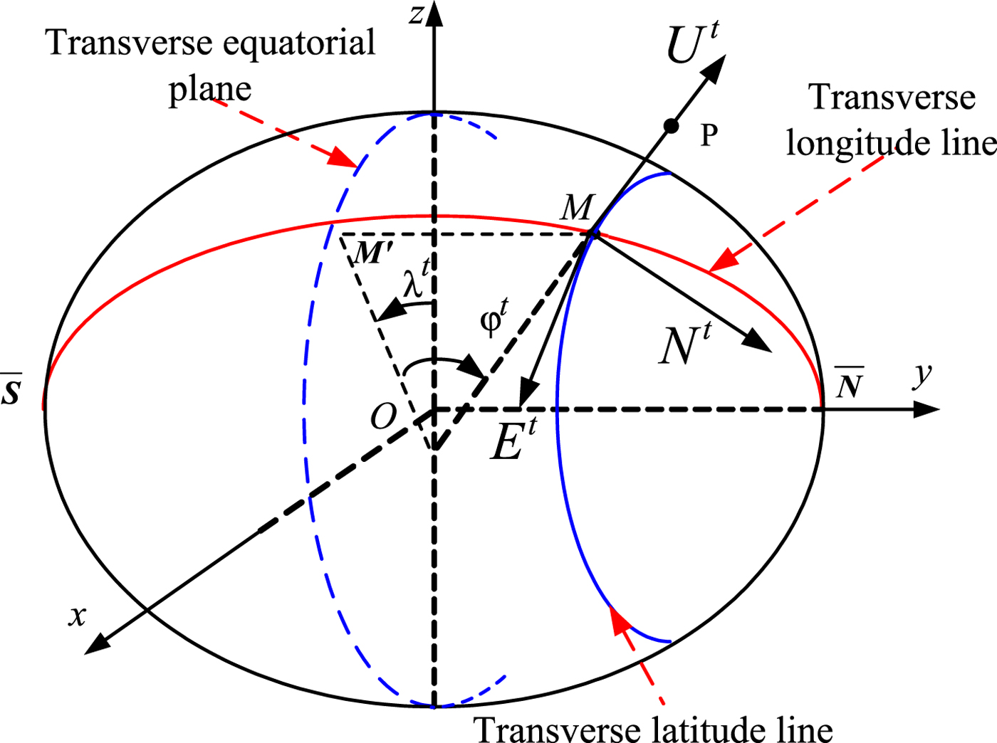
In order to address the problem of traditional inertial navigation methods in the polar regions due to the rapid convergence of meridians, a transversal navigation method was proposed in Broxmeyer (Reference Broxmeyer1964), which transforms the traditional geographic coordinate system into a transversal coordinate system. The original geographical north and south poles are transformed to be the equator in the new coordinate system, as shown in Figure 1.

Figure 1. Transversal Navigation Coordinate System.
Let the transversal coordinate system be e t. The origin of the coordinate system is located at the centre of the Earth O, with the x et axis along the Earth rotation axis, the y et axis along the intersection of the meridian (east meridian 0°) and the z et axis completes the right-handed orthogonal frame. As shown in Figure 1, the relationship between the transversal coordinate system e t and the Earth coordinate system e is given by:
 $${\bf C}_e^{e^t} = \left[\matrix{0 & 0 & 1 \cr 1 & 0 & 0 \cr 0 & 1 & 0} \right]$$
Let the transversal navigation coordinate system be t. Its origin is located at the position of the carrier, the E t axis lies along the tangent of the transversal latitude circle toward the transversal east, the N t axis lies along the tangent of the transversal meridian circle toward the transversal north and the U t axis lies along the normal of the sphere toward the zenith. The definition of the transversal latitude and longitude is similar to the definition of geometric latitude and longitude. Let the meridional circle where the prime meridian is located be the transversal equator, and the original geographic coordinate points [0°, 90°E] and [0°, 90°W] be the new transversal north and south poles, respectively. The transversal meridian is defined as a contour line by crossing the Earth with the plane through two transversal poles.
M′ is the intersecting point of the transversal equator and the transversal meridian passing through point M. The point M is a point on the surface of the Earth. The cross angle between the geometric normal and the transversal equatorial plane is defined as the transversal latitude φt at point M. The transversal north hemisphere is located in the geographical eastern hemisphere and the transversal south hemisphere is located in the geographical western hemisphere. We define the initial transversal meridian as the northern hemisphere part of the geographical meridional circle where the geo-longitude is 90°E. The cross angle between the transversal meridian surface and the initial transversal meridian is defined as the transversal meridian λt at point M. P represents the position of a vehicle with a height h. The position P can be determined by transversal longitude λt, transversal latitude φt and height h, expressed as (x, y, z) in the Earth coordinate system e and as (φ, λ, h) using the geographic latitude and longitude. For the same point, the transformation formula for (x, y, z) and (φt, λ t, h) is given by:
 $$\left\{\matrix{x = (R_n + h) \cos \varphi^t \sin \lambda^t \hfill \cr y = (R_n + h)\sin \varphi^t \hfill \cr z = [R_n (1 - e^2) + h]\cos \varphi^t \cos \lambda^t \hfill}\right.$$
where R n is the radius of the prime vertical circle and e is the elliptical eccentricity.
The transformation formula between (x, y, z) and (φ, λ, h) is given by:
 $$\left\{\matrix{x = (R_n + h)\cos \varphi \cos \lambda \hfill \cr y = (R_n + h) \cos \varphi \sin \lambda \hfill \cr z = [R_n (1 - e^2) + h]\sin \varphi}\right.$$
According to Equations (2) and (3), the relationships of latitude and longitude between the geographic coordinate system and transversal navigation coordinate system are given by:
 $$\left\{\matrix{\sin \varphi^t = \cos \varphi \sin \lambda \hfill \cr \tan \lambda^t = \cot \varphi \cos \lambda \hfill} \right.$$
 $$\left\{\matrix{\sin \varphi = \cos \varphi^t \cos \lambda^t \cr \tan \lambda = \tan \varphi^t \lambda^t \hfill} \right.$$
As R n cannot be treated as a constant value in the polar region, the relationship between R n and φt, λt becomes:
 $$\eqalign{R_n & = \displaystyle{R_e \over \sqrt {1-e^2\sin^2\varphi}} \cr &= \displaystyle{R_e \over \sqrt{1 - e^2 \cos^2 \varphi^t \cos^2 \lambda^t}}}$$
where R e is the equatorial radius, and is a constant.
The transversal navigation coordinate system t can be obtained by two rotations of the Earth coordinate system as follows:
 $$x - y - z \displaystyle{y - axis \over \lambda^t} x_1 - y_1 - z_1 \displaystyle{-x_1 - axis \over \varphi^t} E^t - N^t - U^t$$
We rotate an angle λt around the y positive axis to obtain the coordinate system (x 1, y 1, z 1). The rotation matrix is:
 $${\bf C}_e^1 = \left[\matrix{\cos \lambda^t & 0 & {-\sin \lambda^t} \cr 0 & 1 & 0 \cr {\sin \lambda^t} & 0 & {\cos \lambda^t}} \right]$$
We then rotate an angle φt around the x 1 axis to obtain the ellipsoidal transversal coordinate system. The rotation matrix is:
 $${\bf C}_1^{\rm t} = \left[\matrix{1 & 0 & 0 \cr 0 & {\cos \varphi^t} & {-\sin \varphi^t} \cr 0 & {\sin \varphi^t} & {\cos \varphi^t}} \right]$$
 Thus, the Direction Cosine Matrix (DCM)  ${\bf C}_{e}^{t}$ is determined:
 $${\bf C}_e^t = {\bf C}_1^t {\bf C}_e^1 = \left[\matrix{{\cos \lambda^t} & 0 & {-\sin \lambda^t} \cr {-\sin \varphi^t \sin \lambda^t} & {cos\varphi^t} & {-\sin \varphi^t\cos \lambda^t} \cr {cos\varphi^t\sin \lambda^t} & {\sin \varphi^t} & {cos\varphi^t\cos \lambda^t}} \right]$$
3. DERIVATION OF TWO IMPORTANT FORMULAE IN TRANSVERSAL NAVIGATION
In order to derive the detailed transversal navigation equations, we firstly determine two important formulae. One is the position differential equation and the other is an equation of the transport rate in transversal navigation. Before the presentation of the explicit form of the following equations, we denote the time differential of one variable as d( · ) = d( · )/dt.
Executing differential operations on both sides of Equation (2) and substituting Equation (5) into the resulting equation gives:
 $$\eqalign{{\bf V}^e &= \left[\matrix{{v_x} & {v_y} & {v_z}} \right]^T = \left[\matrix{dx &dy &dz} \right]^T \cr &=\left[\matrix{{\left( \matrix{\sin \lambda^t\cos \varphi^t\left( {dh-\displaystyle{R_e \left(\matrix{2d\lambda^t e^2 \sin \lambda^t \cos \lambda^t \cos^2 \varphi^t \hfill \cr +\,2d\varphi^t e^2 \cos^2 \lambda^t \sin \varphi^t \cos \varphi^t \hfill} \right)\over 2\lpar {1-e^2\cos^2\lambda^t\cos^2\varphi^t}\rpar^{3/2}}} \right) \hfill \cr +\,d\lambda^t\cos \lambda^t\cos \varphi^t\left( {\displaystyle{R_e \over \sqrt {1-e^2\cos^2 \lambda^t\cos^2\varphi^t} }+h} \right) \hfill \cr -\,d\varphi^t\sin \lambda^t\sin \varphi^t\left( {\displaystyle{R_e \over \sqrt {1-e^2\cos^2(\lambda^t)\cos^2(\varphi^t)} }+h}\right) \hfill} \right)} \cr \left( {\sin \varphi^t\left( {dh-\displaystyle{R_e \left( \matrix{2d\lambda^te^2\sin \lambda^t\cos \lambda^t\cos^2\varphi^t \cr +\,2d\varphi^te^2\cos^2\lambda^t\sin \varphi^t\cos \varphi^t} \right) \over 2\lpar {1-e^2\cos^2\lambda^t\cos^2\varphi^t} \rpar^{3/2}}} \right)}\right.\cr +\left.{d\varphi^t\cos \varphi^t\left( {\displaystyle{R_e \over \sqrt {1-e^2\cos^2\lambda^t\cos^2\varphi^t} }+h} \right)} \right) \cr {\left( \matrix{\cos \lambda^t\cos \varphi^t\left( {dh-\displaystyle{(1-e^2)R_e \left(\matrix{2d\lambda^te^2\sin \lambda^t\cos \lambda^t\cos^2\varphi^t \hfill \cr +\,2d\varphi^te^2\cos^2\lambda^t\sin \varphi^t\cos \varphi^t \hfill} \right) \over 2\lpar {1-e^2\cos^2\lambda^t\cos^2\varphi^t} \rpar^{3/2}}} \right) \hfill \cr -\,d\lambda^t\sin \lambda^t\cos \varphi^t \hfill \cr \left( {\displaystyle{(1-e^2)R_e \over \sqrt {1-e^2\cos^2\lambda^t\cos^2\varphi^t}}+h} \right) \hfill\cr -\,d\varphi^t\cos \lambda^t\sin \varphi^t\left( {\displaystyle{(1-e^2)R_e \over \sqrt {1-e^2\cos^2\lambda^t\cos^2\varphi^t} }+h} \right) \hfill}\right)} \hfill}\right]}$$
According to the transversal coordinate system definition, the velocity vector in the transversal navigation coordinate t can be expressed as a component form:
 $${\bf V}^t = \left[\matrix{v_e^t &v_n^t &v_u^t} \right]$$
where v et, v nt, v ut represent the east velocity, north velocity and vertical velocity in transversal coordinate t, respectively.
According to Equations (8)–(10), the velocity in the transversal navigation coordinate t can be obtained:
 $${\bf V}^t = \left[\matrix{v_e^t &v_n^t &v_u^t} \right]^T = ({\bf C}_e^t){\bf V}^e$$
 $$\eqalign{v_e^t &=-\displaystyle{\left( \matrix{d\lambda^te^2\cos^4\lambda^t\cos^3\varphi^t\left( {h\sqrt {1-e^2\cos^2\lambda^t\cos^2\varphi^t} +R_e } \right)+d\lambda^t\cos^2\lambda^t\cos\varphi^t \hfill \cr \lpar {e^2\sin^2\lambda^t\cos^2\varphi^t-1} \rpar \left( {h\sqrt {1-e^2\cos^2\lambda^t\cos^2\varphi^t} +R_e } \right)+d\lambda^t\sin^2\lambda^t\cos \varphi^t \hfill \cr \left( {(e^2-1)R_e -h\sqrt {1-e^2\cos^2\lambda^t\cos^2\varphi^t} } \right)+d\varphi^te^2R_e \sin \lambda^t\cos \lambda^t\sin \varphi^t \hfill} \right) \over \lpar {1-e^2\cos^2\lambda^t\cos^2\varphi^t} \rpar ^{3/2}} \cr v_n^t &=-\displaystyle{\left( \matrix{e^2\cos (2\lambda^t-2\varphi^t)\left( {d\lambda^tR_e +d\varphi^th \sqrt{1-e^2\cos^2\lambda^t\cos^2\varphi^t} } \right) \hfill \cr -\,d\lambda^te^2R_e \cos (2(\lambda^t+\varphi^t)) \hfill \cr +\,2d\varphi^te^2h\cos (2\varphi^t)\sqrt {1-e^2\cos^2\lambda^t\cos^2\varphi^t} \hfill \cr +\,d\varphi^te^2h\cos (2(\lambda^t+\varphi^t))\sqrt {1-e^2\cos^2\lambda^t\cos^2\varphi^t} \hfill \cr +\,2d\varphi^te^2h\sqrt {1-e^2\cos^2\lambda^t\cos^2\varphi^t} -8d\varphi^th\sqrt{1-e^2\cos^2\lambda^t\cos^2\varphi^t} \hfill \cr +\,2d\varphi^te^2\cos (2\lambda^t)\left( {h\sqrt {1-e^2\cos^2\lambda^t\cos^2\varphi^t} +2R_e \hfill} \right)+4d\varphi^te^2Re-8d\varphi^tR_e} \right) \over 8\lpar {1-e^2\cos^2\lambda^t\cos^2\varphi^t}\rpar ^{3/2}} \cr v_u^t &=dh}$$
If dλ t, dφt, dh are treated as unknown variables in Equation (11), the linear equations determined by Equation (11) are solved, and the position differential equation in the transversal coordinate system can be obtained:
 $$\eqalign{d\lambda^t&=\displaystyle{\left(\matrix{\lpar {v_{et}^{\rm sec} } \varphi^t(e^2 \cos (2(\lambda^t+\varphi^t)) +e^2\cos (2(\lambda^t-\varphi^t)) \cr +\,2e^2\cos (2\varphi^t)+2e^2-8)^2 \cr \left({2e^2h\cos (2\varphi^t)\sqrt {1-e^2\cos^2\lambda^t\cos^2\varphi^t}}\right. \cr +\,e^2h \cos (2(\lambda^t + \varphi^t)) \sqrt{1-e^2\cos^2\lambda^t\cos^2\varphi^t} \cr +\,e^2h\cos (2(\lambda^t-\varphi^t)) \sqrt{1-e^2\cos^2\lambda^t\cos^2\varphi^t} \cr +\,2e^2h \sqrt{1-e^2\cos^2\lambda^t\cos^2\varphi^t} \cr -\,8h \sqrt{1-e^2\cos^2\lambda^t\cos^2\varphi^t} +2e^2\cos (2\lambda^t) \cr \left. \left( {h \sqrt{1-e^2\cos^2\lambda^t\cos^2\varphi^t} +2R_e }\right)+4e^2R_e -8R_e \right)}\right) \over \left(\matrix{{\left( {64\lpar {1-e^2\cos^2\lambda^t\cos^2\varphi^t} \rpar^{3/2}\left( {h \sqrt{1-e^2\cos^2\lambda^t\cos^2\varphi^t} +R_e }\right)\cdot } \right.} \cr \left(\matrix{\left(2e^2h\cos (2\varphi^t) \sqrt{1-e^2\cos^2\lambda^t\cos^2\varphi^t}\right. \hfill \cr +\left.e^2h\cos (2(\lambda^t+\varphi^t)) \sqrt{1-e^2\cos^2\lambda^t\cos^2\varphi^t}\right) \hfill \cr +\,e^2h\cos (2(\lambda^t-\varphi^t)) \sqrt{1-e^2\cos^2\lambda^t\cos^2\varphi^t} \hfill \cr +\,2e^2h \sqrt{1-e^2\cos^2\lambda^t\cos^2\varphi^t} \hfill \cr +\,2e^2h\cos (2\lambda^t) \sqrt{1-e^2\cos^2\lambda^t\cos^2\varphi^t} \hfill \cr -\,8h \sqrt{1-e^2\cos^2\lambda^t\cos^2\varphi^t} +8e^2R_e -8R_e \hfill} \right)}\right)} \cr &-\displaystyle{\matrix{(v_{nt} e^2R_e \sin\lambda^t\cos \lambda^t\sin \varphi^t(e^2\cos (2(\lambda^t+\varphi^t)) \cr +\,e^2\cos (2(\lambda^t-\varphi^t))+2e^2\cos(2\lambda^t)+2e^2\cos (2\varphi^t)+2e^2-8)^2)} \over \left(\matrix{8\lpar {1-e^2\cos^2\lambda^t\cos^2\varphi^t} \rpar^{3/2} \left( {h\sqrt{1-e^2\cos^2\lambda^t\cos^2\varphi^t} +R_e } \right)\cdot \cr \left(\matrix{2e^2h\cos (2\varphi^t) \sqrt{1-e^2\cos^2\lambda^t\cos^2\varphi^t} \cr +\,e^2h\cos(2(\lambda^t+\varphi^t)) \sqrt{1-e^2\cos^2\lambda^t\cos^2\varphi^t} \cr +\,e^2h\cos (2(\lambda^t-\varphi^t)) \sqrt{1-e^2\cos^2\lambda^t\cos^2\varphi^t} \cr +\,2e^2h \sqrt{1-e^2\cos^2\lambda^t\cos^2\varphi^t} \cr +\,2e^2h\cos 2\lambda^t \sqrt{1-e^2\cos^2\lambda^t\cos^2\varphi^t} \cr -\,8h\sqrt{1-e^2\cos^2\lambda^t\cos^2\varphi^t} +8e^2R_e -8R_e}\right)}\right)}}$$
 $$\eqalign{d\varphi^t &= \displaystyle{\lpar 16e^2R_e v_{et} \lpar {1-e^2\cos^2\lambda^t\cos^2 \varphi^t} \rpar^{3/2}\csc \lambda^t\hbox{sec} \lambda^t\sin^2(2\lambda^t) \sin \varphi^t\rpar \over \left(\matrix{\left(\sqrt {1-e^2\cos^2\lambda^t\cos^2\varphi^t} h+R_e\right) \cr (2\cos (2\lambda^t)e^2+2\cos (2\varphi^t)e^2+\cos (2(\lambda^t+\varphi^t))e^2 \cr +\,\cos (2(\lambda^t-\varphi^t))e^2+2e^2-8)\sqrt {1-e^2\cos^2\lambda^t\cos^2\varphi^t} \cos (2\varphi^t)e^2 \cr \lpar {8R_e e^2+2h} +h\sqrt {1-e^2\cos^2\lambda^t\cos^2\varphi^t}\cos (2(\lambda^t+\varphi^t))e^2 \cr +\,h\sqrt {1-e^2\cos^2\lambda^t\cos^2\varphi^t} \cos (2(\lambda^t-\varphi^t))e^2 \cr +\,2h\sqrt {1-e^2\cos^2\lambda^t\cos^2\varphi^t} e^2+2h\cos(2\lambda^t)\sqrt {1-e^2\cos^2\lambda^t\cos^2\varphi^t} e^2 \cr -\left. 8R_e -8h\sqrt{1-e^2\cos^2\lambda^t\cos^2\varphi^t} \right)}\right)} \cr &-\displaystyle{\left(\matrix{4v_{nt} \lpar 1-e^2\cos^2\lambda^t\cos^2\varphi^t\rpar^{3/2}\lpar 6R_e e^2 -2\cos (2\lambda^t) \cr \left(R_e -h\sqrt {1-e^2\cos^2\lambda^t\cos^2\varphi^t}\right)e^2+2R_e \cos (2\varphi^t)e^2 \cr +\,2h\sqrt {1-e^2\cos^2\lambda^t\cos^2\varphi^t} \cos (2\varphi^t)e^2+R_e \cos(2(\lambda^t+\varphi^t))e^2 \cr +\,h\sqrt {1-e^2\cos^2\lambda^t\cos^2\varphi^t}\cos (2(\lambda^t+\varphi^t))e^2 \cr +\,\left( {\sqrt {1-e^2\cos^2\lambda^t\cos^2\varphi^t} h+R_e } \right)\cos(2(\lambda^t-\varphi^t))e^2 \cr +\,2h\sqrt {1-e^2\cos^2\lambda^t\cos^2\varphi^t}e^2 \cr -\left. 8R_e -8h\sqrt {1-e^2\cos^2\lambda^t\cos^2\varphi^t}\right)\csc \lambda^t\hbox{sec} \lambda^t\sin (2\lambda^t)}\right) \over \left(\matrix{\left(\sqrt {1-e^2\cos^2\lambda^t\cos^2\varphi^t} h+R_e \right)(2\cos (2\lambda^t)e^2+2\cos (2\varphi^t)e^2 \cr +\,\cos (2(\lambda^t+\varphi^t))e^2+\cos(2(\lambda^t-\varphi^t))e^2+2e^2-8) \cr \lpar 8R_e e^2+2h \sqrt {1-e^2\cos^2\lambda^t\cos^2\varphi^t}\cos (2\varphi^t)e^2 \cr +\,h\sqrt {1-e^2\cos^2\lambda^t\cos^2\varphi^t} \cos(2(\lambda^t+\varphi^t))e^2 \cr +\,h\sqrt {1-e^2\cos^2\lambda^t\cos^2\varphi^t} \cos (2(\lambda^t-\varphi^t))e^2 \cr +\,2h\sqrt {1-e^2\cos^2\lambda^t\cos^2\varphi^t} e^2+2h\cos(2\lambda^t)\sqrt {1-e^2\cos^2\lambda^t\cos^2\varphi^t} e^2 \cr -\left. 8R_e -8h\sqrt{1-e^2\cos^2\lambda^t\cos^2\varphi^t} \right)}\right)}}$$
 $$dh = v_{ut}$$
According to Equations (12)–(14), we obtain the position differential relationship equation in the transversal navigation system, which relates velocity Vt with λt, φt and h.
According to the rule of the DCM differential equation, we know:
 $$\dot{{\bf C}}_e^t = {\bf C}_e^t [{\bf \omega}_{te}^e \times]$$
where  $[{\bf \omega}_{te}^{e} \times]$ is the skew symmetric DCM corresponding to the angular velocity vector
  ${\bf \omega}_{te}^{e} = \left[\matrix{\omega_{te(x)}^{e} &\omega_{te(y)}^{e} &\omega_{te(z)}^{e}} \right]^{T}$, expressed as:
 $$[{\bf \omega}_{te}^e \times] = \left[\matrix{0 & {-\omega_{te(z)}^e } & {\omega_{te(y)}^e} \cr {\omega_{te(z)}^e} & 0 & {-\omega_{te(x)}^e} \cr {-\omega_{te(y)}^e} &{\omega_{te(x)}^e} & 0}\right]$$
According to the orthogonality of the DCM:
 $$({\bf C}e^t)^{-1} = ({\bf C}_e^t)^T$$
Substituting Equation (8) into Equation (15) yields:
 $$[{{\bf \omega}_{te}^e \times }] =({\bf C}_e^t)^{-1} \dot{{\bf C}}_e^t =\left[\matrix{0 & {d\varphi^t\sin \lambda^t} & {-d\lambda^t} \cr {-d\varphi^t\sin \lambda^t} & 0 & {-d\varphi^t\cos \lambda^t} \cr {-d\lambda^t} & {d\varphi^t\cos \lambda^t} & 0}\right]$$
Then ωett can be determined by Equation (18).
Equations (12)–(14) determine the relationship between the velocity and the position of the vehicle in the transversal coordinate system. Equation (18) determines the relationship between the linear velocity and the relative rotation called transport rate in the transversal coordinate system. The two formulae are the basis for the following transversal navigation mechanism.
 $${\bf \omega}_{et}^t = \left[\matrix{{\omega_{et(x)}^t } & {\omega_{et(y)}^t } & {\omega_{et(z)}^t }}\right] = {\bf C}_e^t (-{\bf \omega}_{te}^e)$$
 $$\eqalign{\omega_{et(x)}^t &=\displaystyle{\left(\matrix{4v_{nt} \lpar 1-e^2\cos^2\lambda^t\cos^2\varphi^t\rpar^{3/2}\lpar 6R_e e^2 -2\cos (2\lambda^t) \cr \left( {R_e -h\sqrt {1-e^2\cos^2\lambda^t\cos^2\varphi^t} } \right)e^2+2R_e \cos (2\varphi^t)e^2 \cr +2h\sqrt {1-e^2\cos^2\lambda^t\cos^2\varphi^t} \cos (2\varphi^t)e^2+R_e \cos (2(\lambda^t+\varphi^t))e^2 \cr +h\sqrt {1-e^2\cos^2\lambda^t\cos^2\varphi^t}\cos (2(\lambda^t+\varphi^t))e^2 \cr +\left(\sqrt {1-e^2\cos^2\lambda^t\cos^2\varphi^t} h+R_e \right)\cos (2\lambda^t-2\varphi^t)e^2 \cr +2h\sqrt {1-e^2\cos^2\lambda^t\cos^2\varphi^t}e^2 \cr \left.-8R_e -8h\sqrt {1-e^2\cos^2\lambda^t\cos^2\varphi^t} \right)\csc \lambda^t\hbox{sec} \lambda^t\sin (2\lambda^t)}\right) \over \left(\matrix{\left(\sqrt {1-e^2\cos^2\lambda^t\cos^2\varphi^t} h+R_e\right)( 2\cos (2\lambda^t)e^2 \cr +2\cos (2\varphi^t)e^2+\cos (2(\lambda^t+\varphi^t)) e^2+\cos (2\lambda^t-2\varphi^t)e^2+2e^2-8 ) \cr \lpar 8R_e e^2+2h \sqrt {1-e^2\cos^2\lambda^t\cos^2\varphi^t} \cos (2\varphi^t)e^2 \cr +h\sqrt {1-e^2\cos^2\lambda^t\cos^2\varphi^t} \cos (2(\lambda^t+\varphi^t))e^2 \cr +h\sqrt {1-e^2\cos^2\lambda^t\cos^2\varphi^t} \cos (2\lambda^t-2\varphi^t) e^2+2h\sqrt {1-e^2\cos^2\lambda^t\cos^2\varphi^t} e^2 \cr +2h\cos (2\lambda^t)\sqrt {1-e^2\cos^2\lambda^t\cos^2\varphi^t}e^2-8R_e \cr -\left.8h\sqrt {1-e^2\cos^2\lambda^t\cos^2\varphi^t} \right)}\right)} \cr &-\displaystyle{16e^2R_e v_{et} \lpar 1-e^2\cos^2\lambda^t\cos^2\varphi^t\rpar ^{3/2}\csc \lambda^t\hbox{sec} \lambda^t\sin^2(2\lambda^t)\sin \varphi^t \over \left(\matrix{\left(\sqrt {1-e^2\cos^2\lambda^t\cos^2\varphi^t} h+R_e \right) (2\cos (2\lambda^t)e^2+2\cos (2\varphi^t)e^2 \cr +\cos (2(\lambda^t+\varphi^t))e^2+\cos (2\lambda^t-2\varphi^t)e^2+2e^2-8 ) \cr \lpar 8R_e e^2+2h \sqrt {1-e^2\cos^2\lambda^t\cos^2\varphi^t} \cos (2\varphi^t)e^2 \cr +h\sqrt {1-e^2\cos^2\lambda^t\cos^2\varphi^t} \cos (2(\lambda^t+\varphi^t))e^2 \cr +h\sqrt {1-e^2\cos^2\lambda^t\cos^2\varphi^t} \cos (2\lambda^t-2\varphi^t)e^2 \cr +2h\sqrt {1-e^2\cos^2\lambda^t\cos^2\varphi^t} e^2+2h\cos (2\lambda^t)\sqrt {1-e^2\cos^2\lambda^t\cos^2\varphi^t} e^2 \cr -\left.8R_e -8h\sqrt{1-e^2\cos^2\lambda^t\cos^2\varphi^t} \right)}\right)}}$$
 $$\eqalign{\omega_{et(y)}^t &=\displaystyle{\left(\matrix{{v_{et} (e^2\cos (2(\lambda^t+\varphi^t))+e^2\cos (2\lambda^t-2\varphi^t)+2e^2\cos (2\varphi^t)+2e^2-8)^2} \cr \left(\matrix{ 2e^2h\cos (2\varphi^t) \sqrt{1-e^2\cos^2\lambda^t\cos^2\varphi^t} \hfill \cr +e^2h\cos(2(\lambda^t+\varphi^t)) \sqrt{1-e^2\cos^2\lambda^t\cos^2\varphi^t} \hfill \cr +e^2h\cos (2\lambda^t-2\varphi^t) \sqrt{1-e^2\cos^2\lambda^t\cos^2\varphi^t} \hfill \cr +2e^2h \sqrt{1-e^2\cos^2\lambda^t\cos^2\varphi^t} -8h \sqrt{1-e^2\cos^2\lambda^t\cos^2\varphi^t} \hfill}\right. \cr \left. +2e^2\cos (2\lambda^t)\left(h \sqrt{1-e^2\cos^2\lambda^t\cos^2\varphi^t} +2R_e \right)+4e^2R_e -8R_e \right)}\right) \over \left(\matrix{64\lpar {1-e^2\cos^2\lambda^t\cos^2\varphi^t} \rpar^{3/2} \left(h \sqrt{1-e^2\cos^2\lambda^t\cos^2\varphi^t} +R_e \right)\cdot \cr \left(\matrix{2e^2h\cos (2\varphi^t) \sqrt{1-e^2\cos^2\lambda^t\cos^2\varphi^t} \cr +e^2h\cos(2(\lambda^t+\varphi^t)) \sqrt{1-e^2\cos^2\lambda^t\cos^2\varphi^t} \cr +e^2h\cos (2\lambda^t-2\varphi^t) \sqrt{1-e^2\cos^2\lambda^t\cos^2\varphi^t} \cr +2e^2h \sqrt{1-e^2\cos^2\lambda^t\cos^2\varphi^t} \cr +2e^2h\cos (2\lambda^t) \sqrt{1-e^2\cos^2\lambda^t\cos^2\varphi^t}\cr -8h \sqrt{1-e^2\cos^2\lambda^t\cos^2\varphi^t} +8e^2R_e -8R_e}\right)}\right)} \cr &-\displaystyle{\matrix{(e^2R_e v_{nt} sin\lambda^t\cos \lambda^t\sin \varphi^t (e^2\cos (2(\lambda^t+\varphi^t))+e^2\cos (2\lambda^t-2\varphi^t)\cr +2e^2\cos(2\lambda^t)+2e^2\cos (2\varphi^t)+2e^2-8)^2)} \over \left(\matrix{8\lpar 1-e^2\cos^2\lambda^t\cos^2\varphi^t\rpar^{3/2} \left(h\sqrt{1-e^2\cos^2\lambda^t\cos^2\varphi^t} +R_e \right. \cr \left(\matrix{ 2e^2h\cos (2\varphi^t) \sqrt{1-e^2\cos^2\lambda^t\cos^2\varphi^t} \hfill \cr +e^2h\cos(2(\lambda^t+\varphi^t)) \sqrt{1-e^2\cos^2\lambda^t\cos^2\varphi^t} \hfill \cr +e^2h\cos (2\lambda^t-2\varphi^t) \sqrt{1-e^2\cos^2\lambda^t\cos^2\varphi^t} \hfill \cr +2e^2h \sqrt{1-e^2\cos^2\lambda^t\cos^2\varphi^t} \hfill}\right. \cr +2e^2h\cos (2\lambda^t) \sqrt{1-e^2\cos^2\lambda^t\cos^2\varphi^t} \cr -\left.8h \sqrt{1-e^2\cos^2\lambda^t\cos^2\varphi^t} +8e^2R_e -8R_e\right)}\right)}}$$
 $$\eqalign{\omega_{et(z)}^t &=\displaystyle{\left(\matrix{v_{et} \tan \varphi^t(e^2\cos (2(\lambda^t+\varphi^t))+e^2\cos (2\lambda^t-2\varphi^t) \cr +2e^2\cos (2\lambda^t)+2e^2\cos (2\varphi^t)+2e^2-8)^2 \cr \left(\matrix{2e^2h\cos (2\varphi^t)\sqrt {1-e^2\cos^2\lambda^t\cos^2\varphi^t} \hfill \cr +e^2h\cos(2(\lambda^t+\varphi^t))\sqrt {1-e^2\cos^2\lambda^t\cos^2\varphi^t} \hfill \cr +e^2h\cos (2\lambda^t-2\varphi^t)\sqrt {1-e^2\cos^2\lambda^t\cos^2\varphi^t} \hfill \cr +2e^2h\sqrt {1-e^2\cos^2\lambda^t\cos^2\varphi^t} \hfill}\right. \cr -8h\sqrt {1-e^2\cos^2\lambda^t\cos^2\varphi^t} +2e^2\cos(2\lambda^t) \cr \left.\left(h\sqrt {1-e^2\cos^2\lambda^t\cos^2\varphi^t} +2R_e\right)+4e^2R_e -8R_e \right)}\right) \over \left(\matrix{{64\lpar {1-e^2\cos^2\lambda^t\cos^2\varphi^t} \rpar^{3/2} \left({h\sqrt {1-e^2\cos^2\lambda^t\cos^2\varphi^t} +Re} \right)\cdot } \cr {\left(\matrix{2e^2h\cos (2\varphi^t)\sqrt {1-e^2\cos^2\lambda^t\cos^2\varphi^t} \cr +e^2h\cos (2(\lambda^t+\varphi^t))\sqrt {1-e^2\cos^2\lambda^t\cos^2\varphi^t} \cr +e^2h\cos (2\lambda^t-2\varphi^t)\sqrt {1-e^2\cos^2\lambda^t\cos^2\varphi^t} \cr +2e^2h\sqrt {1-e^2\cos^2\lambda^t\cos^2\varphi^t} \cr +2e^2h\cos (2\lambda^t)\sqrt {1-e^2\cos^2\lambda^t\cos^2\varphi^t} \cr -8h\sqrt {1-e^2\cos^2\lambda^t\cos^2\varphi^t} +8e^2R_e -8R_e}\right)}}\right)} \cr &-\displaystyle{\matrix{(e^2R_e v_{nt} \sin\lambda^t\cos \lambda^t\sin \varphi^t\tan \varphi^t(e^2\cos (2(\lambda^t+\varphi^t))+e^2\cos (2\lambda^t-2\varphi^t) \cr +2e^2\cos (2\lambda^t)+2e^2\cos (2\varphi^t)+2e^2-8)^2)} \over \left(\matrix{8\lpar {1-e^2\cos^2\lambda^t\cos^2\varphi^t} \rpar^{3/2} \cr \left( {h\sqrt{1-e^2\cos^2\lambda^t\cos^2\varphi^t} +R_e } \right. \cr \left(\matrix{2e^2h\cos (2\varphi^t)\sqrt {1-e^2\cos^2\lambda^t\cos^2\varphi^t} \hfill \cr +e^2h\cos(2(\lambda^t+\varphi^t))\sqrt {1-e^2\cos^2\lambda^t\cos^2\varphi^t} \hfill \cr +e^2h\cos (2\lambda^t-2\varphi^t)\sqrt {1-e^2\cos^2(\lambda^t)\cos^2\varphi^t} \hfill \cr +2e^2h\sqrt {1-e^2\cos^2\lambda^t\cos^2\varphi^t} \hfill}\right. \cr +2e^2h\cos (2\lambda^t)\sqrt {1-e^2\cos^2\lambda^t\cos^2\varphi^t} \cr -\left.8h\sqrt {1-e^2\cos^2\lambda^t\cos^2\varphi^t} +8e^2R_e -8R_e \right)}\right)}}$$
4. DIFFERENTIAL EQUATIONS OF ATTITUDE, VELOCITY AND POSITION FOR TRANSVERSAL NAVIGATION
4.1 Differential equation of attitude
The differential equation of attitude matrix Cbt is given by:
 $$\dot{\bf C}_b^t = {\bf C}_b^t ({\bf \omega}_{tb}^t\times)$$
where b is the body coordinate system.
In order to solve this differential equation, we must know the rotation rate ω′tb which is calculated by ωibb, ωiet and ωett as follows:
 $${\bf \omega}_{tb}^b = {\bf \omega}_{ib}^b - {\bf C}_t^b ({\bf \omega}_{ie}^t + {\bf \omega}_{et}^t)$$
where ωibb is the actual measurement of the gyroscope. ωiet is the rotation rate of the Earth and can be determined by:
 $${\bf \omega}_{ie}^t ={\bf C}_e^t {\bf \omega}_{ie} = [{-\sin \lambda^t\omega_{ie} -\sin \varphi^t\cos \lambda^t\omega_{ie} \cos \varphi^t\cos \lambda^t\omega_{ie}}]^T$$
ωett is the key to the attitude solution in transversal navigation, which is already known from Equation (19).
4.2 Differential equation of velocity
In the ellipsoidal transversal coordinate system, the transversal velocity equation can be obtained as follows:
 $$\dot{{\bf V}}^t ={\bf C}_b^t {\bf f}^b-(2{\bf \omega}_{ie}^t +{\bf \omega}_{et}^t)\times {\bf V}^t +{\bf g}^t$$
where Vt is the transversal velocity and gt is the gravitational acceleration vector expressed in the t coordinate. ωiet and ωett can be determined by Equations (22) and (19).
According the definition of transversal navigation coordinate t in Section 2, it is also a horizontal coordinate system, therefore:
 $${\bf g}^t = {\bf g}^n$$
4.3 Differential equation of position
Considering the coupling of the motion in the transversal coordinate system, the differential equations of position are determined by Equations (12) and (13). Since an INS cannot independently determine the vertical position h without external reference information sources (such as an altimeter), the differential equation of vertical position can be removed.
It is well known that in a traditional INS, latitude is only determined by the change rate of north velocity and longitude is only determined by the change rate of east velocity. From Equations (12) and (13), it can be seen that in the transversal coordinate system t, latitude φt and longitude λt are affected by both north velocity v nt and east velocity v et. It can be concluded that there are coupling motions in transversal navigation, which are totally different from a traditional INS.
5. SIMULATION TEST ANALYSIS
In order to verify the feasibility and effectiveness of the proposed navigation scheme, a simulation study was carried out. The trajectory generator was designed as follows: the initial geographical position is (70°N, 0°E) and geographic east velocity and north velocity are both 6 m/s. The heaving motion of the vehicle was set as H · sin(ω · t), where the heave cycle ω = 2π/3600(rad/s) and the heave amplitude H was set as 1 m, 5 m, 10 m, 15 m and 20 m, respectively. The corresponding values are H 1=1, H 2=5, H 3=10, H 4=15, H 5=20. The geographical heading angle was 45°, roll angle was set to 5°sin(πt/4) and the pitch angle was set to 3°cos(πt/5). The simulation period was 24 hours. The proposed transversal navigation mechanism in this paper is called “mechanism 1” and the transversal navigation mechanism proposed in Li et al. (Reference Li, Ben, Yu and Tan2016) is called “mechanism 2”. Both were tested in the simulation experiments. It was found that with the increase of the heaving motions, the principle errors gradually increase, among which the errors of velocity and horizontal attitude are more obviously amplified, as shown in Figure 2 (for brevity, only the curves of east velocity and pitch errors are presented). In Figure 2(a), δV et01, δV et05, δV et10, δV et15, δV et20 are east velocity errors and Φnt01, Φnt05, Φnt10, Φnt15, Φnt20 are pitch errors in the t coordinate system, under the conditions of heaving motion with, H 1=1, H 2=5, H 3=10, H 4=15, H 5=20 respectively.
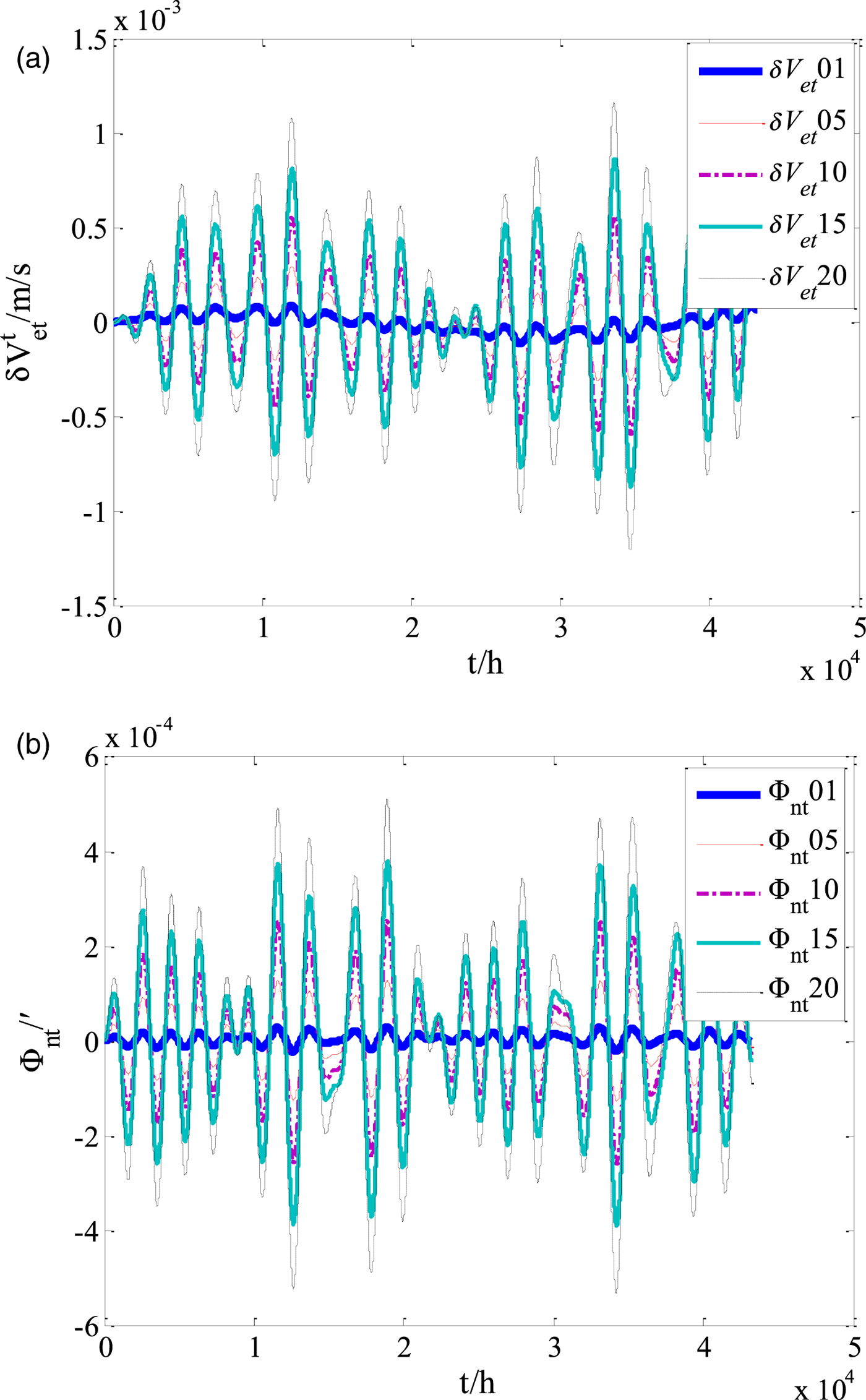
Figure 2. (a) Curves of east velocity error (“mechanism 2”). (b) Curves of pitch error (“mechanism 2”).
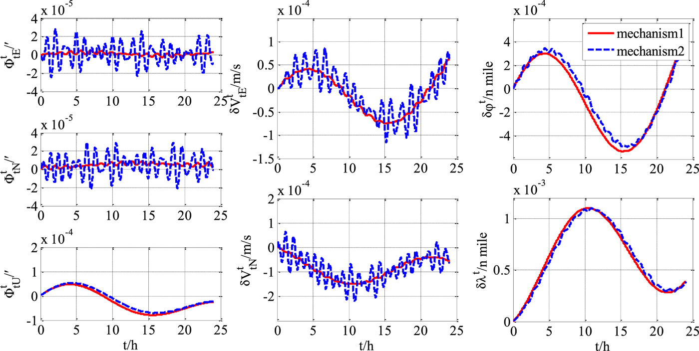
Compared with “mechanism 2”, the precision advantages of “mechanism 1” in position, velocity and attitude error are obviously shown in Figures 3–5 (for brevity, only three cases of curves are given).

Figure 3. Transversal navigation errors (H 1=1).
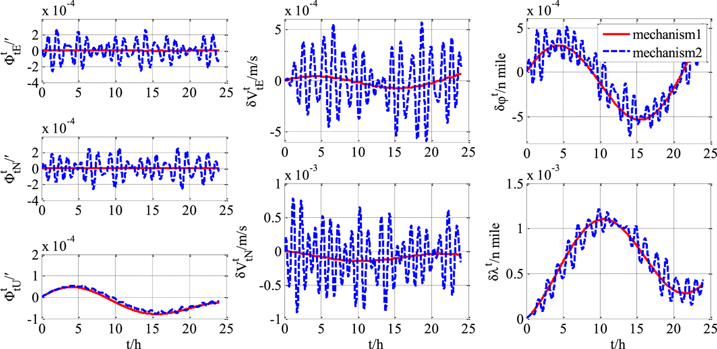
Figure 4. Transversal navigation errors (H 3=10).
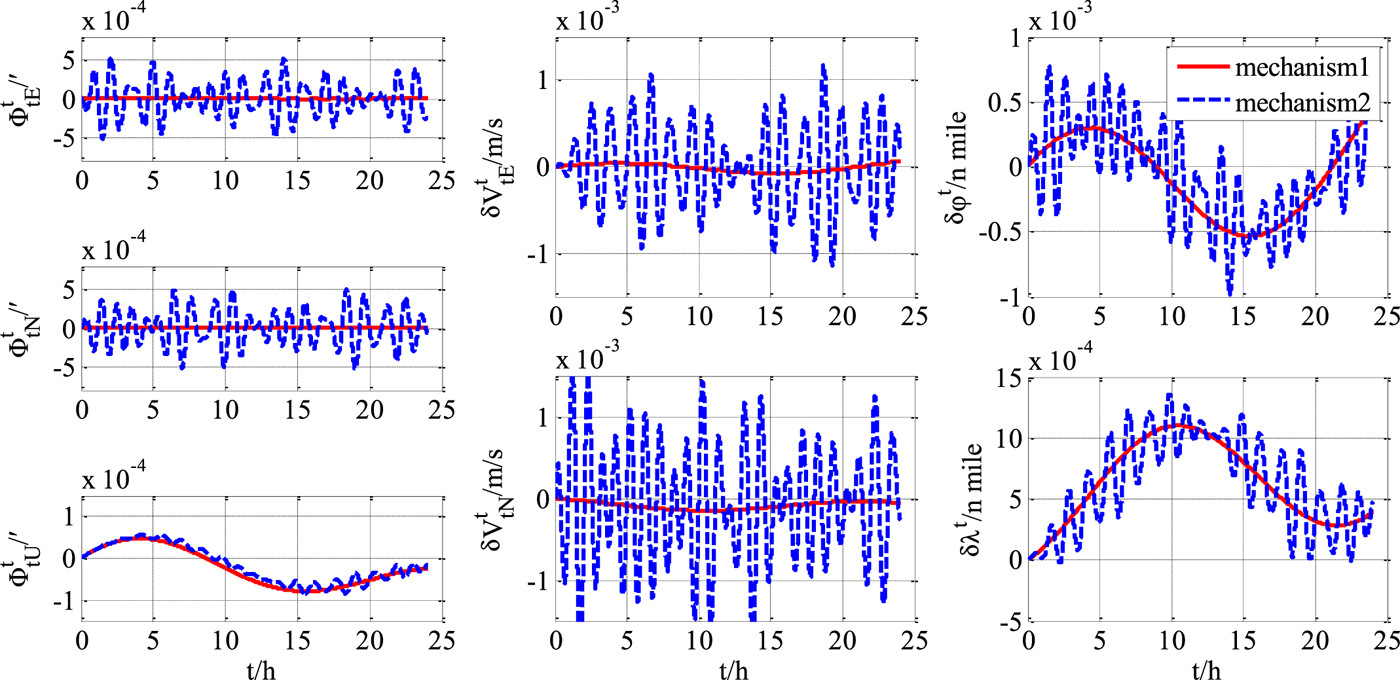
Figure 5. Transversal navigation errors (H 5=20).
Next, some gyroscope and accelerometer errors were introduced, and simulations were repeated. It was found that the proposed improved navigation mechanism still has a precision advantage compared with “mechanism 2” under exactly the same experimental conditions (gyro drifts εx = εy = εz = 0 · 0001°/h, accelerometer biases ∇x=∇y=∇z=10−7g), as shown in Figures 6–8. However, it can be deduced that when the inertial sensor errors become the dominating error sources, the performance improvement using the improved mechanism will be less obvious.
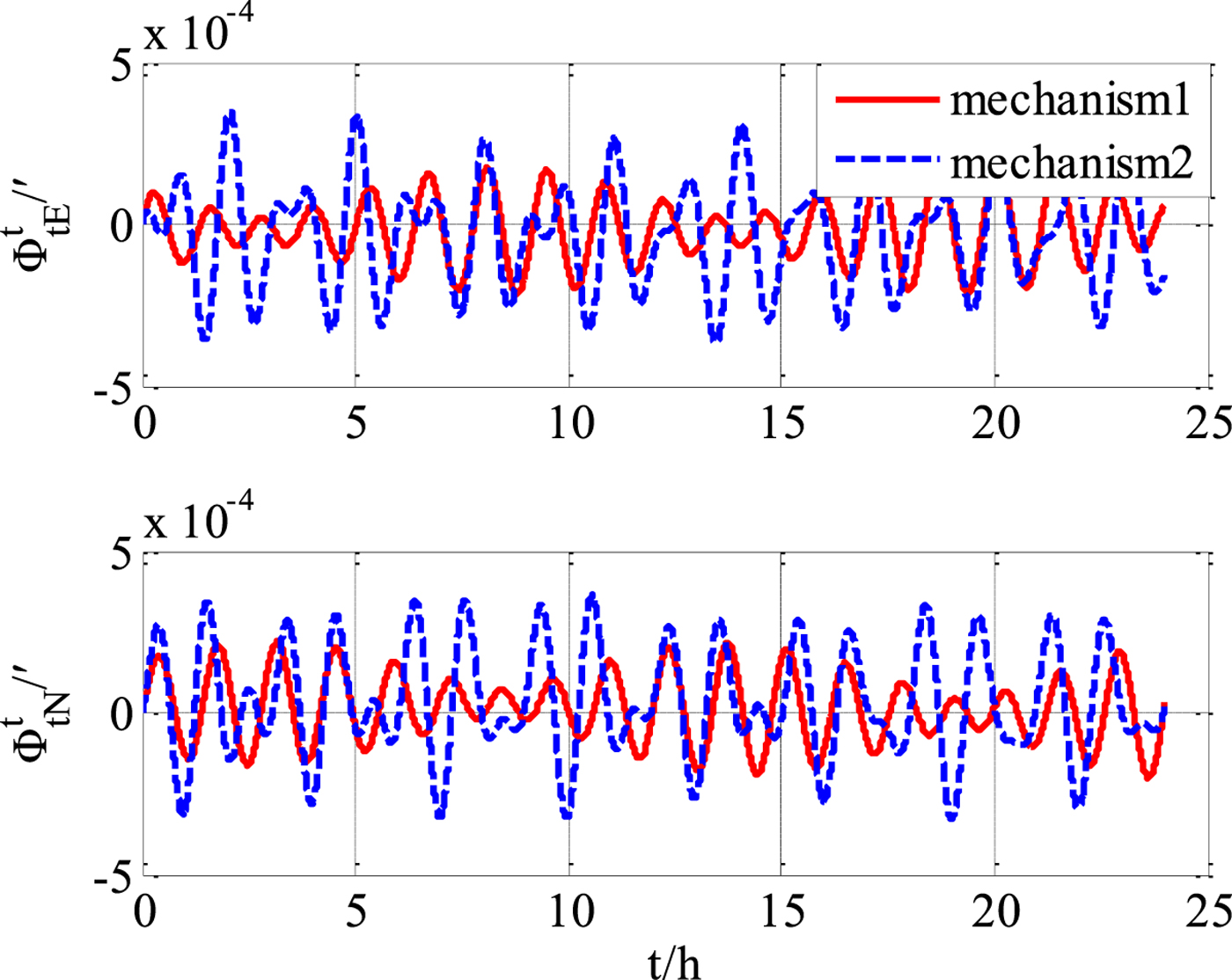
Figure 6. Transversal attitude errors (with gyroscope and accelerometer errors).
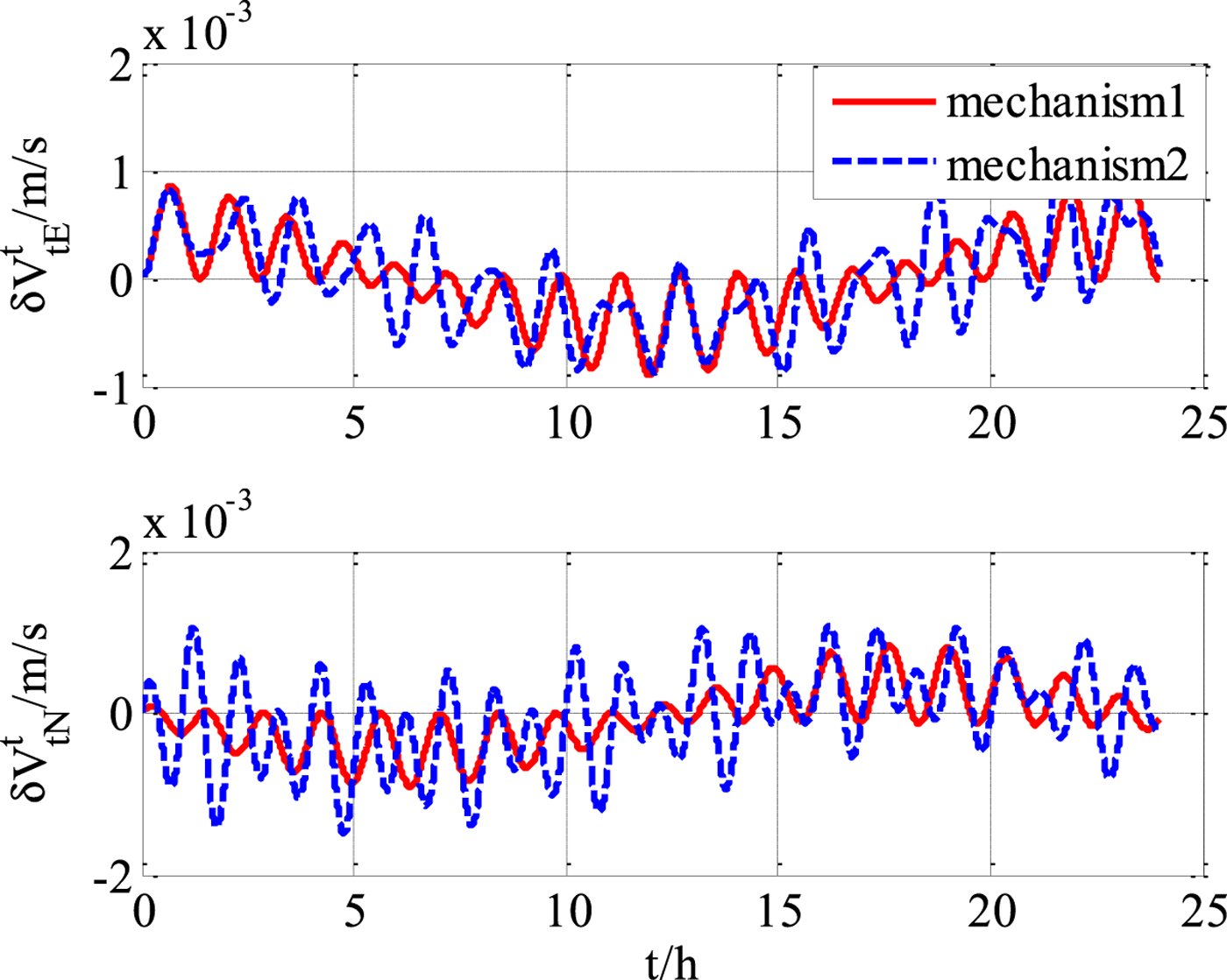
Figure 7. Transversal velocity errors (with gyroscope and accelerometer errors).
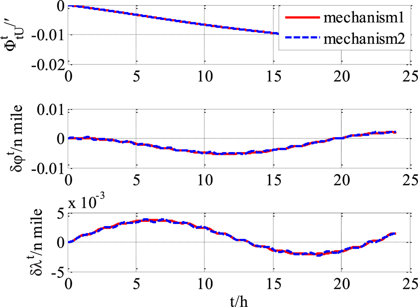
Figure 8. Transversal heading and position errors (with gyroscope and accelerometer errors).
From the experimental results, it can be concluded that the transversal navigation mechanism (“mechanism 2”) presented in Li et al. (Reference Li, Ben, Yu and Tan2016) has errors in the presence of obvious heaving motion, and the performance will deteriorate with motion intensity increases. Errors of horizontal velocity and horizontal attitude are obviously affected by the heaving motion, and the effect on the errors of the position and heading are relatively small. The more rigorous improved mechanism of this paper (“mechanism 1”) has an obvious precision advantage over “mechanism 2”. As the intensity of heaving motion increases, the advantages will increase further.
6. CONCLUSIONS
The traditional transversal navigation algorithm incorporates errors by adopting a simplified Earth model. Establishing an accurate ellipsoid model with elliptic curvature radius can significantly reduce the transversal navigation principle errors. After theoretical analysis by rigorous transversal navigation equations, it is found that under the ellipsoid Earth model, the transversal navigation of the polar region is a complex coupling problem. In this paper, the mechanism of transversal polar region navigation based on an ellipsoidal Earth model is theoretically re-derived, and the complete mechanical arrangement of attitude, position and velocity calculation is presented. The new derivation in this paper completely avoids solving the ellipsoidal radius, and the coupling of the three-dimensional motion is fully considered. The simulation experiment validates the precision advantage of the transversal navigation mechanism proposed in this paper, especially in the condition of vertical motion.
ACKNOWLEDGMENTS
This paper is supported in part by the National Natural Science Foundation of China (61304241 and 61374206) and the National Postdoctoral Program for Innovative Talents (BX 201600038). We would like to thank the anonymous reviewers for their inspirational and valuable suggestions. We have comprehensively re-derived the mechanism of the transversal navigation and re-tested the simulations according to their suggestions.