


1 Introduction
One of the most fascinating features of insects is the reciprocating flapping motion of their wings. The flapping motion is generally a combination of wing translation (yaw) and rotation, where the rotation can be further decomposed into wing pitch and roll. The scientific study of insect flight dates back to the time Chabrier (Reference Chabrier1822) published a book on insect flight and related morphology. However, Hoff (Reference Hoff1919) was probably the first to analyse the aerodynamics of insect flight with momentum theory which idealizes the stroke plane as an actuator disk to continuously impart downward momentum to the air. Since then, aerodynamic modelling of the force generation by flapping wings, especially in an analytical way, has been a research focus for both biologists and engineers. Analytical modelling of flapping wing performance can be roughly classified into three groups: steady-state models, (semi-empirical) quasi-steady models and unsteady models. Steady-state models, including the actuator-disk model (Hoff Reference Hoff1919), provided us with the first insight into the average lift generation and power consumption of flapping flight without digging into the time course of the transient forces (see Weis-Fogh Reference Weis-Fogh1972 and Ellington Reference Ellington1984b ). Meanwhile, quasi-steady models were investigated by Osborne (Reference Osborne1951) and Ellington (Reference Ellington1984a ) by taking the change of the angle of attack (AOA) over time and the velocity variation along the wing span into consideration. Then, with the help of experimental studies on dynamically scaled mechanical flapping wings, empirical corrections were introduced into quasi-steady models to improve their accuracy. Typically these models are refereed to as semi-empirical quasi-steady models (e.g. Dickinson, Lehmann & Sane Reference Dickinson, Lehmann and Sane1999; Berman & Wang Reference Berman and Wang2007). Recently, unsteady models attempted to analytically model the unsteady flow phenomena, for instance, the generation and shedding of leading-edge vortices (LEVs) and trailing-edge vortices (TEVs) (Ansari Reference Ansari2004; Xia & Mohseni Reference Xia and Mohseni2013). These models are capable of demonstrating details of the changing flow field during flapping flight with much less computational cost as compared to the numerical simulations which directly solve the governing Navier–Stokes equations. The Kutta condition is generally enforced at the trailing edge by these unsteady models. However, as pointed out by Ansari, Bikowski & Knowles (Reference Ansari, Bikowski and Knowles2006), during stroke reversals the fluid is more likely to flow around the trailing edge rather than along it such that the applicability of the Kutta condition in the conventional sense is questionable.
With the emergence of flapping wing micro air vehicles (FWMAVs), design studies on flapping wings have stimulated research to keep improving existing quasi-steady models by capturing more unsteady characteristics of prescribed flapping motion without increasing the computational cost. Reviews on recent progress can be found in many papers (Sane Reference Sane2003; Ansari et al. Reference Ansari, Bikowski and Knowles2006; Shyy et al. Reference Shyy, Aono, Chimakurthi, Trizila, Kang, Cesnik and Liu2010). However, the pitching motion of flapping wings of insects, especially during wing reversals, is not always actively controlled. The torsional wave along the trailing edge (TE) of a wing travelling from the wing tip to root is considered as a signature of passive or partly passive wing pitching and has been observed on wings of Diptera (Ennos Reference Ennos1989) and dragonflies (Bergou, Xu & Wang Reference Bergou, Xu and Wang2007). To simplify the drive mechanism, wings of FWMAVs are also designed to pitch passively (Bolsman, Goosen & van Keulen Reference Bolsman, Goosen and van Keulen2009; de Croon et al. Reference de Croon, de Clercq, Ruijsink, Remes and de Wagter2009; Ma et al. Reference Ma, Chirarattananon, Fuller and Wood2013). In this case, the pitching motion is governed by the wing flexibility, inertia and aerodynamic loads.
To study the passive pitching motion and help the wing design, both the aerodynamic force and torque must be calculated. Nevertheless, most existing quasi-steady models are only interested in, and limited to, the prediction of the force generation. On the other hand, there are some attempts to model the torque in order to study the passive pitching behaviour. For example, Bergou et al. (Reference Bergou, Xu and Wang2007) employed a quasi-steady model to verify if sufficient pitching torque could be generated to realize passive wing reversals. The aerodynamic force on the wing was calculated based on the formulas used for studying fluttering and tumbling plates (Andersen, Pesavento & Wang Reference Andersen, Pesavento and Wang2005). To predict the passive pitching motion over an entire stroke, Whitney & Wood (Reference Whitney and Wood2010) used a quasi-steady model that includes the aerodynamic loads due to the wing translation, rotation and the added-mass effect with the help of some empirical coefficients. They pointed out that the effect of the coupling between wing translation and rotation was not included in their model since the corresponding centre of pressure (CP) is hard to determine analytically due to the unsteadiness introduced by the wing rotation. However, experiments conducted by Sane & Dickinson (Reference Sane and Dickinson2002) show that the coupling effect and the position of the pitching axis (as shown in figure 1) have a big influence on the aerodynamic loads generated by flapping wings. Consequently, both should be included in the quasi-steady aerodynamic model. Another common limitation of most existing quasi-steady models is the heavy dependence on empirical parameters. Those parameters need to be determined by experiments each time the wing shape is changed. This hinders their application to wing design and optimization.

Figure 1. Illustration of the pitching axis of a flapping wing. In lateral view on the right, the filled circle in grey represents the leading edge (LE) of the wing, and
 $\hat{d}$
indicates the dimensionless distance from the LE to the pitching axis.
$\hat{d}$
indicates the dimensionless distance from the LE to the pitching axis.
In the present work, we propose a more comprehensive and predictive quasi-steady model by including four aerodynamic loading terms that result from the wing’s translation, rotation, their coupling as well as the added-mass effect. In § 2, we demonstrate the necessity of including all the four terms for a quasi-steady model in order to predict both the aerodynamic force and torque accurately. In § 3, two validations are used to show the capability and accuracy of the proposed model to predict the CP, aerodynamic loads and passive pitching motion by comparing with experimental data and other existing quasi-steady models. Conclusions are provided in § 4.
2 Formulation
The reciprocating flapping motion is the most prominent feature of flapping wings, which sets it apart from other traditional methods of flight. The flapping motion results in large geometrical AOA which would stall conventional translating wings. For flapping wings, generally, the flow starts to separate at the LE after wing reversals, and forms a LEV or LEVs (Johansson et al. Reference Johansson, Engel, Kelber, Heerenbrink and Hedenström2013). Instead of growing quickly and then shedding into the wake, the LEV on flapping wings generally remains attached over the entire half-strokes for two possible reasons: (i) the spanwise flow from the wing root to tip removes energy from the LEV which limits the growth and the shedding, as shown on Hawkmoth wings (Ellington et al. Reference Ellington, van den Berg, Willmott and Thomas1996); and (ii) due to the downwash flow induced by the tip and wake vortices, the effective AOA decreases and the growth of the LEV is restricted, as indicated by the wings of Drosophila (Birch & Dickinson Reference Birch and Dickinson2001). The prolonged attachment of the LEV assists flapping wings to maintain high lift. This phenomenon makes it more convenient to analytically model the aerodynamic effect of the attached LEV compared to the case that the LEV sheds before the pitching reversal.
To analytically predict the unsteady aerodynamic loads on flapping wings, we presume the following.
-
(i) The flow is incompressible, i.e. the fluid density
 ${\it\rho}^{f}$
is regarded as a constant. This is justified due to the relative low average wing tip velocity compared to the speed of sound (Sun Reference Sun2014).
${\it\rho}^{f}$
is regarded as a constant. This is justified due to the relative low average wing tip velocity compared to the speed of sound (Sun Reference Sun2014). -
(ii) The wing is a rigid, flat plate. Wings of some small insects (e.g. fruit-fly wings (Ellington Reference Ellington1999)) and FWMAV wings (Ma et al. Reference Ma, Chirarattananon, Fuller and Wood2013) show negligible wing deformation. Even for wings of larger insects, the enhancement of lift due to wing camber and twisting is generally less than 10 % compared to their rigid counterparts (Sun Reference Sun2014). The wing thickness
$t$
is also negligible when compared to the other two dimensions, i.e. the average chord length
$\bar{c}$
and span
$R$
(see figure 1). -
(iii) The resultant aerodynamic force acting on the wing is perpendicular to the chord during the entire stroke. This assumption is supported by three facts: (a) the leading-edge suction force (Sane Reference Sane2003) is negligible for a plate with negligible thickness; (b) the viscous drag on the wing surface is marginal as compared to the dominant pressure load when moving at a post-stall AOA; (c) the strength of the bound circulation, which results in a net force perpendicular to the incoming flow, is negligible as compared to the vorticity-induced circulation (Ford & Babinsky Reference Ford and Babinsky2014).
-
(iv) A quasi-steady state is assumed for an infinitesimal duration such that the transient loads on the flapping wing are equivalent to those for steady motion at the same instantaneous translational velocity, angular velocity and AOA.


Considering the variation in the velocity and acceleration along the wing span, the blade-element method (BEM) (Osborne Reference Osborne1951) is used for discretizing the wing into chordwise strips with finite width. The resultant loads can be calculated by integrating strip loads over the entire wing. As a consequence of the quasi-steady assumption, the time dependence of the aerodynamic loads primarily arises from the time-varying kinematics.
2.1 Flapping kinematics
To describe the kinematics of a rigid flapping wing, three successive rotations, i.e. sweeping motion (yaw), heaving motion (roll) and pitching motion (pitch), are used, as illustrated by the ‘cans in series’ diagram in figure 2. Four different frames are involved in these rotations, including inertial frame
 $x_{i}y_{i}z_{i}$
, two intermediate frames
$x_{i}y_{i}z_{i}$
, two intermediate frames
 $x_{{\it\theta}}y_{{\it\theta}}z_{{\it\theta}}$
and
$x_{{\it\theta}}y_{{\it\theta}}z_{{\it\theta}}$
and
 $x_{{\it\eta}}y_{{\it\eta}}z_{{\it\eta}}$
and co-rotating frame
$x_{{\it\eta}}y_{{\it\eta}}z_{{\it\eta}}$
and co-rotating frame
 $x_{c}y_{c}z_{c}$
. The inertial frame
$x_{c}y_{c}z_{c}$
. The inertial frame
 $x_{i}y_{i}z_{i}$
is fixed at the joint that connects the wing to the body of FWMAVs. Axes
$x_{i}y_{i}z_{i}$
is fixed at the joint that connects the wing to the body of FWMAVs. Axes
 $x_{i}$
and
$x_{i}$
and
 $y_{i}$
confine the stroke plane while the
$y_{i}$
confine the stroke plane while the
 $z_{i}$
axis is perpendicular to this plane and follows the right-hand rule which holds for all the frames. The rotation around the
$z_{i}$
axis is perpendicular to this plane and follows the right-hand rule which holds for all the frames. The rotation around the
 $z_{i}$
axis represents the sweeping motion and results in the intermediate frame
$z_{i}$
axis represents the sweeping motion and results in the intermediate frame
 $x_{{\it\theta}}y_{{\it\theta}}z_{{\it\theta}}$
. The heaving motion is the rotation around the
$x_{{\it\theta}}y_{{\it\theta}}z_{{\it\theta}}$
. The heaving motion is the rotation around the
 $y_{{\it\theta}}$
axis and leads to another intermediate frame
$y_{{\it\theta}}$
axis and leads to another intermediate frame
 $x_{{\it\eta}}y_{{\it\eta}}z_{{\it\eta}}$
, where the pitching motion is conducted about its
$x_{{\it\eta}}y_{{\it\eta}}z_{{\it\eta}}$
, where the pitching motion is conducted about its
 $x_{{\it\eta}}$
axis. Eventually, we get the co-rotating frame
$x_{{\it\eta}}$
axis. Eventually, we get the co-rotating frame
 $x_{c}y_{c}z_{c}$
, which is fixed to and co-rotates with the wing. Its
$x_{c}y_{c}z_{c}$
, which is fixed to and co-rotates with the wing. Its
 $x_{c}$
axis coincides with the pitching axis, and the
$x_{c}$
axis coincides with the pitching axis, and the
 $z_{c}$
axis coincides with the wing plane and perpendicular to the
$z_{c}$
axis coincides with the wing plane and perpendicular to the
 $x_{c}$
axis. Both the inertial frame
$x_{c}$
axis. Both the inertial frame
 $x_{i}y_{i}z_{i}$
and the co-rotating frame
$x_{i}y_{i}z_{i}$
and the co-rotating frame
 $x_{c}y_{c}z_{c}$
are of particular interest for the study of flapping wing motion and aerodynamic performance. The quasi-steady aerodynamic model presented in this work is constructed in the co-rotating frame in order to facilitate the application of the BEM, while the lift and drag are generally quantified in the inertial frame.
$x_{c}y_{c}z_{c}$
are of particular interest for the study of flapping wing motion and aerodynamic performance. The quasi-steady aerodynamic model presented in this work is constructed in the co-rotating frame in order to facilitate the application of the BEM, while the lift and drag are generally quantified in the inertial frame.

Figure 2. Successive wing rotations used to describe the kinematics of a rigid flapping wing, shown using the ‘cans in series’ approach proposed by Schwab & Meijaard (Reference Schwab and Meijaard2006). Four different frames are involved in these rotations, including inertial frame
 $x_{i}y_{i}z_{i}$
, two intermediate frames
$x_{i}y_{i}z_{i}$
, two intermediate frames
 $x_{{\it\theta}}y_{{\it\theta}}z_{{\it\theta}}$
and
$x_{{\it\theta}}y_{{\it\theta}}z_{{\it\theta}}$
and
 $x_{{\it\eta}}y_{{\it\eta}}z_{{\it\eta}}$
and co-rotating frame
$x_{{\it\eta}}y_{{\it\eta}}z_{{\it\eta}}$
and co-rotating frame
 $x_{c}y_{c}z_{c}$
. All these frames share the same origin although they are drawn at various locations.
$x_{c}y_{c}z_{c}$
. All these frames share the same origin although they are drawn at various locations.
The flapping motion can be quantified using three Euler angles: sweeping angle
 ${\it\phi}$
, heaving angle
${\it\phi}$
, heaving angle
 ${\it\theta}$
and pitching angle
${\it\theta}$
and pitching angle
 ${\it\eta}$
. An example of these Euler angles during flapping motion has been demonstrated in a semi-sphere constructed in the inertial frame, as shown in figure 3. It can been seen that
${\it\eta}$
. An example of these Euler angles during flapping motion has been demonstrated in a semi-sphere constructed in the inertial frame, as shown in figure 3. It can been seen that
 ${\it\phi}$
is the angle between the
${\it\phi}$
is the angle between the
 $x_{i}$
axis and the projection of the
$x_{i}$
axis and the projection of the
 $x_{c}$
axis on the stroke plane,
$x_{c}$
axis on the stroke plane,
 ${\it\theta}$
is the angle between the
${\it\theta}$
is the angle between the
 $x_{c}$
axis and its projection on the stroke plane, and
$x_{c}$
axis and its projection on the stroke plane, and
 ${\it\eta}$
is the angle between the
${\it\eta}$
is the angle between the
 $z_{c}$
axis and the plane that is perpendicular to the stroke plane and parallel to the
$z_{c}$
axis and the plane that is perpendicular to the stroke plane and parallel to the
 $x_{c}$
axis. With these Euler angles, three successive rotations, i.e. the sweeping, heaving and pitching motion, can be formulated as
$x_{c}$
axis. With these Euler angles, three successive rotations, i.e. the sweeping, heaving and pitching motion, can be formulated as
 $$\begin{eqnarray}\unicode[STIX]{x1D64D}_{{\it\phi}}=\left[\begin{array}{@{}ccc@{}}\cos {\it\phi} & -\sin \,{\it\phi} & 0\\ \sin {\it\phi} & \cos {\it\phi} & 0\\ 0 & 0 & 1\end{array}\right],\quad \unicode[STIX]{x1D64D}_{{\it\theta}}=\left[\begin{array}{@{}ccc@{}}\cos {\it\theta} & 0 & \sin {\it\theta}\\ 0 & 1 & 0\\ -\sin \,{\it\theta} & 0 & \cos {\it\theta}\end{array}\right],\quad \unicode[STIX]{x1D64D}_{{\it\eta}}=\left[\begin{array}{@{}ccc@{}}1 & 0 & 0\\ 0 & \cos {\it\eta} & -\sin \,{\it\eta}\\ 0 & \sin {\it\eta} & \cos {\it\eta}\end{array}\right]\!,\end{eqnarray}$$
respectively.

Figure 3. Two frames and three Euler angles demonstrated in a semi-sphere. Frames
 $x_{i}y_{i}z_{i}$
and
$x_{i}y_{i}z_{i}$
and
 $x_{c}y_{c}z_{c}$
are fixed to the origin and co-rotates with the wing, respectively. Axes
$x_{c}y_{c}z_{c}$
are fixed to the origin and co-rotates with the wing, respectively. Axes
 $x_{i}$
and
$x_{i}$
and
 $y_{i}$
confine the stroke plane. The small circles indicate the wing tip trajectory (‘
$y_{i}$
confine the stroke plane. The small circles indicate the wing tip trajectory (‘
 $\infty$
’ shape here as an example). The plane constructed by the dashed lines is perpendicular to the stroke plane and parallels to the
$\infty$
’ shape here as an example). The plane constructed by the dashed lines is perpendicular to the stroke plane and parallels to the
 $x_{c}$
axis.
$x_{c}$
axis.
 ${\it\phi}$
,
${\it\phi}$
,
 ${\it\theta}$
and
${\it\theta}$
and
 ${\it\eta}$
represent the sweeping, heaving and pitching angle, respectively.
${\it\eta}$
represent the sweeping, heaving and pitching angle, respectively.
The quasi-steady model proposed in this work calculates the aerodynamic loads in the co-rotating frame. Therefore, the velocity and acceleration information in the co-rotating frame are required. The angular velocity
 ${\bf\omega}_{c}$
and angular acceleration
${\bf\omega}_{c}$
and angular acceleration
 ${\bf\alpha}_{c}$
can be obtained by transforming the sweeping and heaving motions from corresponding frames into the co-rotating frame where the wing pitching motion is described, as in,
${\bf\alpha}_{c}$
can be obtained by transforming the sweeping and heaving motions from corresponding frames into the co-rotating frame where the wing pitching motion is described, as in,
 $$\begin{eqnarray}{\bf\omega}_{c}=\unicode[STIX]{x1D64D}_{{\it\eta}}^{\text{T}}\unicode[STIX]{x1D64D}_{{\it\theta}}^{\text{T}}\unicode[STIX]{x1D64D}_{{\it\phi}}^{\text{T}}\dot{{\it\phi}}\boldsymbol{e}_{z_{i}}+\unicode[STIX]{x1D64D}_{{\it\eta}}^{\text{T}}\unicode[STIX]{x1D64D}_{{\it\theta}}^{\text{T}}\dot{{\it\theta}}\boldsymbol{e}_{y_{{\it\theta}}}+\unicode[STIX]{x1D64D}_{{\it\eta}}^{\text{T}}\dot{{\it\eta}}\boldsymbol{e}_{x_{{\it\eta}}}=\left[\begin{array}{@{}c@{}}\dot{{\it\eta}}-\dot{{\it\phi}}\sin {\it\theta}\\ \dot{{\it\theta}}\cos {\it\eta}+\dot{{\it\phi}}\cos {\it\theta}\sin {\it\eta}\\ \dot{{\it\phi}}\cos {\it\eta}\cos {\it\theta}-\dot{{\it\theta}}\sin {\it\eta}\end{array}\right],\end{eqnarray}$$
and
 $$\begin{eqnarray}{\bf\alpha}_{c}=\dot{{\bf\omega}}_{c}=\left[\begin{array}{@{}c@{}}\ddot{{\it\eta}}-\ddot{{\it\phi}}\sin {\it\theta}-\dot{{\it\phi}}\dot{{\it\theta}}\cos {\it\theta}\\ \ddot{{\it\phi}}\cos {\it\theta}\sin {\it\eta}+\ddot{{\it\theta}}\cos {\it\eta}-\dot{{\it\eta}}\dot{{\it\theta}}\sin {\it\eta}+\dot{{\it\phi}}(\dot{{\it\eta}}\cos {\it\eta}\cos {\it\theta}-\dot{{\it\theta}}\sin {\it\eta}\sin {\it\theta})\\ \ddot{{\it\phi}}\cos {\it\eta}\cos {\it\theta}-\ddot{{\it\theta}}\sin {\it\eta}-\dot{{\it\eta}}\dot{{\it\theta}}\cos {\it\eta}-\dot{{\it\phi}}(\dot{{\it\eta}}\cos {\it\theta}\sin {\it\eta}+\dot{{\it\theta}}\cos {\it\eta}\sin {\it\theta})\end{array}\right],\end{eqnarray}$$
where
 $\boldsymbol{e}_{z_{i}}$
,
$\boldsymbol{e}_{z_{i}}$
,
 $\boldsymbol{e}_{y_{{\it\theta}}}$
and
$\boldsymbol{e}_{y_{{\it\theta}}}$
and
 $\boldsymbol{e}_{x_{{\it\eta}}}$
are unit vectors in the directions of
$\boldsymbol{e}_{x_{{\it\eta}}}$
are unit vectors in the directions of
 $z_{i}$
,
$z_{i}$
,
 $y_{{\it\theta}}$
and
$y_{{\it\theta}}$
and
 $x_{{\it\eta}}$
axis, respectively.
$x_{{\it\eta}}$
axis, respectively.
In the co-rotating frame, the translational velocity and acceleration of a point on the pitching axis with a position vector
 $\boldsymbol{r}=[x_{c},0,0]^{\text{T}}$
can be calculated by
$\boldsymbol{r}=[x_{c},0,0]^{\text{T}}$
can be calculated by
 $$\begin{eqnarray}\boldsymbol{v}_{c}={\bf\omega}_{c}\times \boldsymbol{r}=x_{c}[0,{\it\omega}_{z_{c}},-{\it\omega}_{y_{c}}]^{\text{T}},\end{eqnarray}$$
and
 $$\begin{eqnarray}\boldsymbol{a}_{c}={\bf\alpha}_{c}\times \boldsymbol{r}+{\bf\omega}_{c}\times \boldsymbol{v}_{c}=x_{c}[-{\it\omega}_{y_{c}}^{2}-{\it\omega}_{z_{c}}^{2},{\it\alpha}_{z_{c}}+{\it\omega}_{x_{c}}{\it\omega}_{y_{c}},{\it\omega}_{x_{c}}{\it\omega}_{z_{c}}-{\it\alpha}_{y_{c}}]^{\text{T}},\end{eqnarray}$$
where the term
 ${\bf\omega}_{c}\times \boldsymbol{v}_{c}$
represents the Coriolis effect due to the rotation of the co-rotating frame.
${\bf\omega}_{c}\times \boldsymbol{v}_{c}$
represents the Coriolis effect due to the rotation of the co-rotating frame.
Given the kinematic information, we are able to determine the aerodynamic loads on a flapping wing during hovering. If, instead, the forward flight is studied, the contribution of the velocity of forward flight to the resultant translational velocity has to be included. This can be done by transforming the forward velocity from the inertial frame to the co-rotating frame and then adding this to the translational velocity
 $\boldsymbol{v}_{c}$
as formulated in (2.4).
$\boldsymbol{v}_{c}$
as formulated in (2.4).
2.2 Aerodynamic modelling
For flapping wings, it is attractive to model the aerodynamic loads analytically since the numerical simulations by directly solving the governing Navier–Stokes equations are extremely time consuming and also require a comprehensive representation of the flow physics for high accuracy. The design and optimization of flapping wings for FWMAVs also demand an efficient tool to quickly evaluate the aerodynamic performance of given designs.

Figure 4. Decomposition of total aerodynamic loads on a flapping wing. The wing kinematic quantities and aerodynamic forces are illustrated qualitatively. The grey line segments, grey dots, larger white circles and black dots represent the chord, LE, pitching axis and chord centre, respectively. The smaller white circles indicate the locations of centre of pressure/load induced by each term.
As a result of the unsteadiness of the fluid surrounding flapping wings, it is non-trivial to analytically formulate the total aerodynamic load in a single term. Instead, we separate it into four parts: the translation-induced load, the rotation-induced load, the load resulting from the coupling between the wing translation and rotation and the load due to the added-mass effect, as illustrated in figure 4. The first three components represent the pressure loads induced by the translational and/or rotational velocities while the added-mass effect results from the energy dissipation or absorption by the fluid that is decelerated or accelerated by the flapping wing. The contribution of added-mass effect to the resultant aerodynamic load relies on the values of translational and rotational acceleration as well as the location of rotation axis, which are normally represented by the matrix of added-mass coefficients. These coefficients for two-dimensional plates have been well studied (Newman Reference Newman1977) and thus are used in this model by combining with the BEM. However, different combinations of the first three terms can be found in the literature depending on the problem studied. In table 1, we compare two quasi-steady models (Berman & Wang Reference Berman and Wang2007; Whitney & Wood Reference Whitney and Wood2010) which have been commonly used with the proposed model on four aspects: (i) capability of predicting the resultant force and torque, (ii) composition of the resultant loads, (iii) whether a real pitching axis position is used and (iv) dependence on empirical parameters. For flapping wings with fully prescribed kinematics, generally, the desired information is the (average) aerodynamic force. The rotation-induced force is ignored in these cases for two reasons: (i) the transient force due to pure rotation will be zero if the wing platform is symmetric about the pitching axis, which is generally assumed (Berman & Wang Reference Berman and Wang2007), (ii) the average force due to the pure rotation over one flapping cycle is zero if its two half-strokes mirror each other. For flapping wings with passive pitching motion, both the temporal aerodynamic force and torque are required to calculate the pitching motion. The contribution of the pure wing rotation has to be considered since the distributed damping load due to wing rotation always adds a torque about the pitching axis no matter if the net force is zero or not. However, the coupling effect between the translation and rotation of the wing is generally ignored (Whitney & Wood Reference Whitney and Wood2010) or considered without taking the pitching axis into consideration (Bergou et al. Reference Bergou, Xu and Wang2007). This is because of the difficulty in analytically determining the contribution of wing rotation to the aerodynamic loads due to the unsteadiness. It can be seen that existing quasi-steady models show inconsistency in the loading terms that are included. Therefore, this work aims to achieve a better quasi-steady model from the perspectives of:
-
(i) eliminating the inconsistency in the loading terms;
-
(ii) modelling the total contribution of the wing rotation to the resultant aerodynamic loads and corresponding CP more accurately;
-
(iii) and further reducing the dependence on empirical parameters.
Table 1. Comparison of the characteristics between two existing quasi-steady models and the proposed model; ‘—’ means that the resultant torque estimation was not the objective of the model of Berman & Wang (Reference Berman and Wang2007) and thus not present in their paper.

In the following subsections, the components as listed in figure 4 will be elucidated in sequence. After that, the Wagner effect (Wagner Reference Wagner1925) and corresponding conditions under which it should be considered are discussed.
2.2.1 Translation-induced load
Experimental studies (Ellington et al.
Reference Ellington, van den Berg, Willmott and Thomas1996; Pitt Ford & Babinsky Reference Pitt Ford and Babinsky2013; Percin & van Oudheusden Reference Percin and van Oudheusden2015) show that the LEV dominates the force generation of translational wings compared to the bound circulation. Due to the unsteadiness of the LEV, the translational lift coefficient
 $C_{L}^{\mathit{trans}}$
is generally measured on dynamically scaled flapping wings. According to experimental results obtained on different wings (Dickinson et al.
Reference Dickinson, Lehmann and Sane1999; Usherwood & Ellington Reference Usherwood and Ellington2002b
; Wang, Birch & Dickinson Reference Wang, Birch and Dickinson2004), the lift coefficient can be approximately formulated as
$C_{L}^{\mathit{trans}}$
is generally measured on dynamically scaled flapping wings. According to experimental results obtained on different wings (Dickinson et al.
Reference Dickinson, Lehmann and Sane1999; Usherwood & Ellington Reference Usherwood and Ellington2002b
; Wang, Birch & Dickinson Reference Wang, Birch and Dickinson2004), the lift coefficient can be approximately formulated as
 $$\begin{eqnarray}C_{L}^{\mathit{trans}}=A\sin (2\tilde{{\it\alpha}}),\end{eqnarray}$$
where
 $A$
is the maximum lift coefficient to be determined experimentally for different wings, and the AOA (
$A$
is the maximum lift coefficient to be determined experimentally for different wings, and the AOA (
 $\tilde{{\it\alpha}}$
) for a rigid wing model can be calculated by
$\tilde{{\it\alpha}}$
) for a rigid wing model can be calculated by
 $$\begin{eqnarray}\tilde{{\it\alpha}}=\arccos (|v_{z_{c}}/v_{c}|)=\arccos \left(\left|{\it\omega}_{y_{c}}\Big/\sqrt{{\it\omega}_{y_{c}}^{2}+{\it\omega}_{z_{c}}^{2}}\right|\right),\quad \text{if }\boldsymbol{v}_{c}\neq \mathbf{0}.\end{eqnarray}$$
According to equation (2.6), the wing translating at an AOA of
 $45^{\circ }$
gives the maximum lift, but the maximum value
$45^{\circ }$
gives the maximum lift, but the maximum value
 $A$
might differ from one wing to the other. The experimental determination of
$A$
might differ from one wing to the other. The experimental determination of
 $A$
hinders a general application to calculate the lift coefficient of arbitrary wings. Based on the extended lift line theory (Schlichting & Truckenbrodt Reference Schlichting and Truckenbrodt1979) for low-aspect-ratio wings in an incompressible flow, Taha, Hajj & Beran (Reference Taha, Hajj and Beran2014) used an analytical expression for the coefficient
$A$
hinders a general application to calculate the lift coefficient of arbitrary wings. Based on the extended lift line theory (Schlichting & Truckenbrodt Reference Schlichting and Truckenbrodt1979) for low-aspect-ratio wings in an incompressible flow, Taha, Hajj & Beran (Reference Taha, Hajj and Beran2014) used an analytical expression for the coefficient
 $A$
of a flat flapping wing. That is
$A$
of a flat flapping wing. That is
 $$\begin{eqnarray}\begin{array}{@{}c@{}}\end{array}\end{eqnarray}$$
where ![]() is the aspect ratio, defined as
is the aspect ratio, defined as
 $R/\bar{c}$
. Using (2.8), rather good estimations of the lift coefficients for translational flapping wings with different aspect ratios can be achieved according to the comparison with experimental data (see Taha et al. (Reference Taha, Hajj and Beran2014)).
$R/\bar{c}$
. Using (2.8), rather good estimations of the lift coefficients for translational flapping wings with different aspect ratios can be achieved according to the comparison with experimental data (see Taha et al. (Reference Taha, Hajj and Beran2014)).
It should be noted that
 $C_{L}^{\mathit{trans}}$
is the three-dimensional (3-D) lift coefficient for the entire wing. However, it is more useful to know the 2-D coefficient (
$C_{L}^{\mathit{trans}}$
is the three-dimensional (3-D) lift coefficient for the entire wing. However, it is more useful to know the 2-D coefficient (
 $C_{l}^{\mathit{trans}}$
) for the wing airfoil that can be used directly in the BEM. Conventionally, the translational velocity at the radius of gyration is taken as the reference to calculate the aerodynamic forces for the entire flapping wings (e.g. Harbig, Sheridan & Thompson Reference Harbig, Sheridan and Thompson2014; Lee, Choi & Kim Reference Lee, Choi and Kim2015; Percin & van Oudheusden Reference Percin and van Oudheusden2015). In this case, the same resultant translational lift can be obtained by BEM with
$C_{l}^{\mathit{trans}}$
) for the wing airfoil that can be used directly in the BEM. Conventionally, the translational velocity at the radius of gyration is taken as the reference to calculate the aerodynamic forces for the entire flapping wings (e.g. Harbig, Sheridan & Thompson Reference Harbig, Sheridan and Thompson2014; Lee, Choi & Kim Reference Lee, Choi and Kim2015; Percin & van Oudheusden Reference Percin and van Oudheusden2015). In this case, the same resultant translational lift can be obtained by BEM with
 $C_{l}^{\mathit{trans}}$
which takes the value of
$C_{l}^{\mathit{trans}}$
which takes the value of
 $C_{L}^{\mathit{trans}}$
, as shown in appendix A. Therefore,
$C_{L}^{\mathit{trans}}$
, as shown in appendix A. Therefore,
 $C_{L}^{\mathit{trans}}$
is directly used in our quasi-steady model to evaluate the translational aerodynamic forces.
$C_{L}^{\mathit{trans}}$
is directly used in our quasi-steady model to evaluate the translational aerodynamic forces.
According to the assumption that the resultant force is perpendicular to the wing surface (i.e. aligned with the
 $y_{c}$
axis), the translational drag and resultant force coefficients can be calculated by using the translational lift coefficient as formulated in (2.6), as given by
$y_{c}$
axis), the translational drag and resultant force coefficients can be calculated by using the translational lift coefficient as formulated in (2.6), as given by
 $$\begin{eqnarray}C_{D}^{\mathit{trans}}=C_{L}^{\mathit{trans}}\tan (\tilde{{\it\alpha}})\end{eqnarray}$$
and
 $$\begin{eqnarray}C_{F_{y_{c}}}^{\mathit{ trans}}=C_{L}^{\mathit{trans}}/\cos (\tilde{{\it\alpha}}).\end{eqnarray}$$
Using equations (2.6), (2.9) and (2.10), we calculate the analytical lift, drag and resultant force coefficients as a function of the AOA for a dynamically scaled Hawkmoth wing (Usherwood & Ellington Reference Usherwood and Ellington2002a
) and Drosophila wing (Dickinson et al.
Reference Dickinson, Lehmann and Sane1999), respectively, as shown in figure 5(a). The order of magnitudes of the Reynolds number of the Hawkmoth wing ![]() and Drosophila wing
and Drosophila wing ![]() are
are
 $10^{3}$
and
$10^{3}$
and
 $10^{2}$
, respectively. Comparison of the polar plots based on the analytical and experimental results is given in figure 5(b). It can be seen that the analytical lift and drag coefficients agree with the experimental results very well for both wings except for the discrepancy at the pre-stall AOAs (i.e.
$10^{2}$
, respectively. Comparison of the polar plots based on the analytical and experimental results is given in figure 5(b). It can be seen that the analytical lift and drag coefficients agree with the experimental results very well for both wings except for the discrepancy at the pre-stall AOAs (i.e.
 $0^{\circ }{-}20^{\circ }$
) for the Drosophila wing. The discrepancy is mainly because of the neglected viscous drag at the boundary layer in the proposed model while the drag does exist in reality, especially at small Reynolds number and low AOA. However, the AOA of flapping wings is normally in the post-stall region. Therefore, it is acceptable to use the analytical formulas to predict the force coefficients of translational wings.
$0^{\circ }{-}20^{\circ }$
) for the Drosophila wing. The discrepancy is mainly because of the neglected viscous drag at the boundary layer in the proposed model while the drag does exist in reality, especially at small Reynolds number and low AOA. However, the AOA of flapping wings is normally in the post-stall region. Therefore, it is acceptable to use the analytical formulas to predict the force coefficients of translational wings.

Figure 5. Force coefficients of two different translational wings. HM and DS represent dynamically scaled wings by mimicking wings of Hawkmoth (Usherwood & Ellington Reference Usherwood and Ellington2002a
) and Drosophila (Dickinson et al.
Reference Dickinson, Lehmann and Sane1999), respectively. (a) Analytical lift, drag and resultant force coefficients calculated with (2.6), (2.9) and (2.10). (b) Comparison of analytical and measured force coefficients represented by polar plots which show the relationship between the translation-induced lift and drag coefficients at AOAs ranging from
 $0^{\circ }$
to
$0^{\circ }$
to
 $90^{\circ }$
in
$90^{\circ }$
in
 $5^{\circ }$
and
$5^{\circ }$
and
 $4.5^{\circ }$
increments for the HM and DS wings, respectively.
$4.5^{\circ }$
increments for the HM and DS wings, respectively.
The resultant wing translation-induced force
 $F_{y_{c}}^{\mathit{trans}}$
can be calculated by integrating over the wing surface as in
$F_{y_{c}}^{\mathit{trans}}$
can be calculated by integrating over the wing surface as in
 $$\begin{eqnarray}F_{y_{c}}^{\mathit{ trans}}=-\text{sgn}({\it\omega}_{z_{c}})\frac{1}{2}{\it\rho}^{f}({\it\omega}_{y_{c}}^{2}+{\it\omega}_{z_{c}}^{2})C_{F_{y_{c}}}^{\mathit{ trans}}\int _{0}^{R}x_{c}^{2}c\,\text{d}x_{c},\end{eqnarray}$$
where
 $\text{sgn}(\cdot )$
is the signum function and
$\text{sgn}(\cdot )$
is the signum function and
 $c$
is the chord length as a function of the radius
$c$
is the chord length as a function of the radius
 $x_{c}$
. The translational velocity
$x_{c}$
. The translational velocity
 $v_{c}$
shown in figure 4 is written as
$v_{c}$
shown in figure 4 is written as
 $x_{c}\sqrt{{\it\omega}_{y_{c}}^{2}+{\it\omega}_{z_{c}}^{2}}$
. It should be noted that the angular velocity has been taken out of the integration based on the rigid wing assumption.
$x_{c}\sqrt{{\it\omega}_{y_{c}}^{2}+{\it\omega}_{z_{c}}^{2}}$
. It should be noted that the angular velocity has been taken out of the integration based on the rigid wing assumption.
Experimental measurements of the CP on flapping wings that translate at different AOAs have been conducted by Dickson et al. (Reference Dickson, Straw, Poelma and Dickinson2006) on a dynamically scaled Drosophila wing and by Han et al. (Reference Han, Kim, Chang and Han2015) on a Hawkmoth wing. The measured chordwise CP locations
 $\hat{d}_{cp}^{\mathit{trans}}$
for both Hawkmoth and Drosophila wing, which have been normalized by local chord length, are linearly fitted and plotted as a function of AOA in figure 6. Both lines show the shift of the CP from near the LE (
$\hat{d}_{cp}^{\mathit{trans}}$
for both Hawkmoth and Drosophila wing, which have been normalized by local chord length, are linearly fitted and plotted as a function of AOA in figure 6. Both lines show the shift of the CP from near the LE (
 $\hat{d}_{cp}^{\mathit{trans}}=0$
) to the chord centre (
$\hat{d}_{cp}^{\mathit{trans}}=0$
) to the chord centre (
 $\hat{d}_{cp}^{\mathit{trans}}=0.5$
) with the increase of AOA. In the proposed model, the value of
$\hat{d}_{cp}^{\mathit{trans}}=0.5$
) with the increase of AOA. In the proposed model, the value of
 $\hat{d}_{cp}^{\mathit{trans}}$
is assumed to be linear to the AOA as given by
$\hat{d}_{cp}^{\mathit{trans}}$
is assumed to be linear to the AOA as given by
 $$\begin{eqnarray}\hat{d}_{cp}^{\mathit{trans}}=\frac{1}{{\rm\pi}}\tilde{{\it\alpha}},\quad \text{where }0\leqslant \tilde{{\it\alpha}}\leqslant \frac{{\rm\pi}}{2},\end{eqnarray}$$
which indicates that the proposed formula assumes that
 $\hat{d}_{cp}^{\mathit{trans}}$
is equal to 0 and 0.5, respectively, when AOA is 0 and
$\hat{d}_{cp}^{\mathit{trans}}$
is equal to 0 and 0.5, respectively, when AOA is 0 and
 ${\rm\pi}/2$
. For the post-stall AOA which is generally experienced by flapping wings, the CP location from the proposed formula almost stays between the empirical data obtained from two model wings.
${\rm\pi}/2$
. For the post-stall AOA which is generally experienced by flapping wings, the CP location from the proposed formula almost stays between the empirical data obtained from two model wings.

Figure 6. Measured chordwise CP for dynamically scaled insect wings and the analytical formula of CP used in our model. The values of CP are normalized by local chords and denoted as
 $\hat{d}_{cp}^{\mathit{trans}}$
.
$\hat{d}_{cp}^{\mathit{trans}}$
.
With the analytical resultant force and the chordwise CP location for translating wings, the torques around the
 $x_{c}$
axis and
$x_{c}$
axis and
 $z_{c}$
axis of the co-rotating frame can be expressed as
$z_{c}$
axis of the co-rotating frame can be expressed as
 $$\begin{eqnarray}{\it\tau}_{x_{c}}^{\mathit{ trans}}=\left\{\begin{array}{@{}ll@{}}\displaystyle -\text{sgn}({\it\omega}_{z_{c}}){\displaystyle \frac{{\it\rho}^{f}}{2}}({\it\omega}_{y_{c}}^{2}+{\it\omega}_{z_{c}}^{2})C_{F_{y_{c}}}^{\mathit{trans}}(\hat{d}_{cp}^{\mathit{trans}}-\hat{d})\int _{0}^{R}x_{c}^{2}c^{2}\,\text{d}x_{c}, & {\it\omega}_{y_{c}}\leqslant 0\\ \displaystyle -\text{sgn}({\it\omega}_{z_{c}}){\displaystyle \frac{{\it\rho}^{f}}{2}}({\it\omega}_{y_{c}}^{2}+{\it\omega}_{z_{c}}^{2})C_{F_{y_{c}}}^{\mathit{trans}}(1-\hat{d}_{cp}^{\mathit{trans}}-\hat{d})\int _{0}^{R}x_{c}^{2}c^{2}\,\text{d}x_{c}, & {\it\omega}_{y_{c}}>0\end{array}\right.\end{eqnarray}$$
and
 $$\begin{eqnarray}{\it\tau}_{z_{c}}^{\mathit{ trans}}=-\text{sgn}({\it\omega}_{z_{c}})\frac{{\it\rho}^{f}}{2}({\it\omega}_{y_{c}}^{2}+{\it\omega}_{z_{c}}^{2})C_{F_{y_{c}}}^{\mathit{ trans}}\int _{0}^{R}x_{c}^{3}c\,\text{d}x_{c},\end{eqnarray}$$
where
 $\hat{d}$
is the normalized distance between the LE and the pitching axis (see figure 1), and the negative and positive values of
$\hat{d}$
is the normalized distance between the LE and the pitching axis (see figure 1), and the negative and positive values of
 ${\it\omega}_{y_{c}}$
mean that the translational velocity component
${\it\omega}_{y_{c}}$
mean that the translational velocity component
 $v_{z_{c}}$
(
$v_{z_{c}}$
(
 $=-x_{c}{\it\omega}_{y_{c}}$
) points at the LE and TE, respectively. When
$=-x_{c}{\it\omega}_{y_{c}}$
) points at the LE and TE, respectively. When
 ${\it\omega}_{y_{c}}>0$
, the real AOA is higher than
${\it\omega}_{y_{c}}>0$
, the real AOA is higher than
 $90^{\circ }$
which is not covered by the analytical model for AOA, as shown in figure 6. This situation is handled by taking the TE as the LE, then the AOA becomes less than
$90^{\circ }$
which is not covered by the analytical model for AOA, as shown in figure 6. This situation is handled by taking the TE as the LE, then the AOA becomes less than
 $90^{\circ }$
. The torque about
$90^{\circ }$
. The torque about
 $y_{c}$
axis is zero since the resultant force is assumed to be perpendicular to the wing.
$y_{c}$
axis is zero since the resultant force is assumed to be perpendicular to the wing.
The translation-induced loads have been analytically represented while taking account of the influence of ![]() . This allows further application to study the wing shape influence in an analytical manner.
. This allows further application to study the wing shape influence in an analytical manner.
2.2.2 Rotation-induced load
When a wing rotates about an arbitrary axis in a medium, it experiences distributed loads. Although the resultant force is zero if the wing is symmetric about its rotation axis, the resultant torque about the rotation axis is non-zero. Therefore, it is necessary to include this rotation-induced load in the quasi-steady model to correctly calculate the aerodynamic torque. In fact, this loading term is excluded by most existing quasi-steady models.
To calculate this load using BEM, the wing has to be discretized into chordwise strips first. For a rotating wing, different velocities are induced in the chordwise direction (
 $=-z_{c}{\it\omega}_{x_{c}}$
), for which the amplitude linearly increases with the distance from the pitching axis. The chordwise velocity gradient requires the discretization of each chordwise strip as well. Consequently, the resultant rotation-induced force is calculated by integrating the load on each infinitesimal area (i.e.
$=-z_{c}{\it\omega}_{x_{c}}$
), for which the amplitude linearly increases with the distance from the pitching axis. The chordwise velocity gradient requires the discretization of each chordwise strip as well. Consequently, the resultant rotation-induced force is calculated by integrating the load on each infinitesimal area (i.e.
 $\text{d}x_{c}\,\text{d}z_{c}$
) over the entire wing surface, as in
$\text{d}x_{c}\,\text{d}z_{c}$
) over the entire wing surface, as in
 $$\begin{eqnarray}F_{y_{c}}^{\mathit{ rot}}=\frac{{\it\rho}^{f}}{2}{\it\omega}_{x_{c}}|{\it\omega}_{x_{c}}|C_{D}^{\mathit{rot}}\int _{0}^{R}\!\int _{\hat{d}c-c}^{\hat{d}c}z_{c}|z_{c}|\text{d}z_{c}\,\text{d}x_{c},\end{eqnarray}$$
where
 $C_{D}^{\mathit{rot}}$
is the rotational damping coefficient,
$C_{D}^{\mathit{rot}}$
is the rotational damping coefficient,
 $\hat{d}c-c$
and
$\hat{d}c-c$
and
 $\hat{d}c$
are the coordinates of the wing’s TE and LE in the
$\hat{d}c$
are the coordinates of the wing’s TE and LE in the
 $z_{c}$
direction, respectively. Meanwhile, the resultant torques around axes
$z_{c}$
direction, respectively. Meanwhile, the resultant torques around axes
 $x_{c}$
and
$x_{c}$
and
 $z_{c}$
are calculated by
$z_{c}$
are calculated by
 $$\begin{eqnarray}{\it\tau}_{x_{c}}^{\mathit{ rot}}=-\frac{{\it\rho}^{f}}{2}{\it\omega}_{x_{c}}|{\it\omega}_{x_{c}}|C_{D}^{\mathit{rot}}\int _{0}^{R}\!\int _{\hat{d}c-c}^{\hat{d}c}|z_{c}|^{3}\text{d}z_{c}\,\text{d}x_{c},\end{eqnarray}$$
and
 $$\begin{eqnarray}{\it\tau}_{z_{c}}^{\mathit{ rot}}=\frac{{\it\rho}^{f}}{2}{\it\omega}_{x_{c}}|{\it\omega}_{x_{c}}|C_{D}^{\mathit{rot}}\int _{0}^{R}\!\int _{\hat{d}c-c}^{\hat{d}c}z_{c}|z_{c}|x_{c}\text{d}z_{c}\,\text{d}x_{c}.\end{eqnarray}$$
This discretization approach was also used by Andersen et al. (Reference Andersen, Pesavento and Wang2005) with a value of 2.0 for
 $C_{D}^{\mathit{rot}}$
on a tumbling plate and by Whitney & Wood (Reference Whitney and Wood2010) with a value of 5.0 for flapping wings to achieve a better agreement between theoretical and experimental results. It is necessary to generalize this coefficient to enable the application for different flapping wings. The damping load on a rotating plate is analogous to the load acting on a plate that is placed vertically in a flow with varying incoming velocities from the top to bottom. The latter is basically the case for a translational wing at an angle of attack of
$C_{D}^{\mathit{rot}}$
on a tumbling plate and by Whitney & Wood (Reference Whitney and Wood2010) with a value of 5.0 for flapping wings to achieve a better agreement between theoretical and experimental results. It is necessary to generalize this coefficient to enable the application for different flapping wings. The damping load on a rotating plate is analogous to the load acting on a plate that is placed vertically in a flow with varying incoming velocities from the top to bottom. The latter is basically the case for a translational wing at an angle of attack of
 $90^{\circ }$
. However, it is questionable if it is sufficient to use the traditional drag coefficient for a pure translating plate normal to flow (
$90^{\circ }$
. However, it is questionable if it is sufficient to use the traditional drag coefficient for a pure translating plate normal to flow (
 ${\approx}2$
for a flat plate at
${\approx}2$
for a flat plate at
 $\mathit{Re}=10^{5}$
(Anderson Reference Anderson2010)). During the wing reversals of flapping motion, the sweeping motion is almost seized but the pitching velocity is nearly maximized. In this case, the pure rotational load dominates the aerodynamic loading which is still influenced by the flow field induced by the past sweeping motion. In this situation, it is more correct to use the translational drag coefficient
$\mathit{Re}=10^{5}$
(Anderson Reference Anderson2010)). During the wing reversals of flapping motion, the sweeping motion is almost seized but the pitching velocity is nearly maximized. In this case, the pure rotational load dominates the aerodynamic loading which is still influenced by the flow field induced by the past sweeping motion. In this situation, it is more correct to use the translational drag coefficient
 $C_{D}^{\mathit{trans}}$
for a sweeping wing (see (2.9)) when AOA is equal to
$C_{D}^{\mathit{trans}}$
for a sweeping wing (see (2.9)) when AOA is equal to
 $90^{\circ }$
as the rotational damping coefficient, i.e.
$90^{\circ }$
as the rotational damping coefficient, i.e.
 $$\begin{eqnarray}\begin{array}{@{}c@{}}\end{array}\end{eqnarray}$$
which normally leads to higher damping coefficients (e.g.
 $C_{D}^{\mathit{rot}}=3.36$
when
$C_{D}^{\mathit{rot}}=3.36$
when ![]() ) as compared to the drag coefficient for a pure translating plate normal to flow.
) as compared to the drag coefficient for a pure translating plate normal to flow.
To avoid alternating the LE during flapping, which increases the power consumption, the pitching axes of flapping wings are generally located between the LE and the centre line (Berman & Wang Reference Berman and Wang2007). The CP location of the load induced by the pure rotation, which is defined as the local chord-length-normalized distance from the LE to the CP, can be determined by
 $$\begin{eqnarray}\hat{d}_{cp}^{\mathit{rot}}=-\frac{3}{4}\frac{(\hat{d}-1)^{4}+\hat{d}^{4}}{(\hat{d}-1)^{3}+\hat{d}^{3}}+\hat{d},\quad \text{where }0\leqslant \hat{d}<0.5,\end{eqnarray}$$
which implies that the CP moves from three-quarters of the chord to infinity while the pitching axis moves from the LE to the chord centre.
2.2.3 Coupling load
Although the translation- and rotation-induced loads have been modelled analytically and separately, they are insufficient to represent the loads on the wing conducting translation and rotation simultaneously because of the nonlinearity introduced by the fluid–wing interaction. Considering a wing whose planform is symmetric about its pitching axis and moving with constant translational and rotational velocities, the resultant rotation-induced force
 $F_{y_{c}}^{\mathit{rot}}$
is equal to zero. The resultant force, therefore, should be equal to the translational force
$F_{y_{c}}^{\mathit{rot}}$
is equal to zero. The resultant force, therefore, should be equal to the translational force
 $F_{y_{c}}^{\mathit{trans}}$
for a linear system assumption. However, for this case, the experiment conducted by Sane & Dickinson (Reference Sane and Dickinson2002) reported a higher resultant force compared to
$F_{y_{c}}^{\mathit{trans}}$
for a linear system assumption. However, for this case, the experiment conducted by Sane & Dickinson (Reference Sane and Dickinson2002) reported a higher resultant force compared to
 $F_{y_{c}}^{\mathit{trans}}$
. This additional force is explained by the coupling effect between the wing translation and rotation.
$F_{y_{c}}^{\mathit{trans}}$
. This additional force is explained by the coupling effect between the wing translation and rotation.
Traditionally, the coupling load on a plate with translational velocity
 $v$
, rotational angular velocity
$v$
, rotational angular velocity
 ${\it\omega}_{x_{c}}$
, chord
${\it\omega}_{x_{c}}$
, chord
 $c$
and unit span is formulated as
$c$
and unit span is formulated as
 $$\begin{eqnarray}F_{\mathit{trad}}^{\mathit{coupl}}={\it\rho}^{f}v\underbrace{C^{\mathit{coupl}}{\it\omega}_{x_{c}}c^{2}({\textstyle \frac{3}{4}}-\hat{d})}_{\mathit{rotational\, circulation}},\end{eqnarray}$$
where
 $C^{\mathit{coupl}}$
is a constant coupling coefficient equal to
$C^{\mathit{coupl}}$
is a constant coupling coefficient equal to
 ${\rm\pi}$
. The term was first included into a quasi-steady model for flapping wings by Ellington (Reference Ellington1984a
) to reflect the contribution of wing rotation on the aerodynamic force. Since then, this term is widely used in quasi-steady analysis (Dickinson et al.
Reference Dickinson, Lehmann and Sane1999; Sane & Dickinson Reference Sane and Dickinson2002; Nabawy & Crowther Reference Nabawy and Crowther2014) for different types of insect wings. It is generally assumed that the contribution of the wing rotation can be represented by this single coupling term without considering the load due to the pure wing rotation. However, there are some limitations for the coupling term to fully represent the rotational effect. Firstly, the coupling coefficient
${\rm\pi}$
. The term was first included into a quasi-steady model for flapping wings by Ellington (Reference Ellington1984a
) to reflect the contribution of wing rotation on the aerodynamic force. Since then, this term is widely used in quasi-steady analysis (Dickinson et al.
Reference Dickinson, Lehmann and Sane1999; Sane & Dickinson Reference Sane and Dickinson2002; Nabawy & Crowther Reference Nabawy and Crowther2014) for different types of insect wings. It is generally assumed that the contribution of the wing rotation can be represented by this single coupling term without considering the load due to the pure wing rotation. However, there are some limitations for the coupling term to fully represent the rotational effect. Firstly, the coupling coefficient
 $C^{\mathit{coupl}}$
in (2.20) is a constant, but experiments (Sane & Dickinson Reference Sane and Dickinson2002; Han et al.
Reference Han, Kim, Chang and Han2015) have shown its dependency on the ratio between the translational velocity
$C^{\mathit{coupl}}$
in (2.20) is a constant, but experiments (Sane & Dickinson Reference Sane and Dickinson2002; Han et al.
Reference Han, Kim, Chang and Han2015) have shown its dependency on the ratio between the translational velocity
 $v$
and rotational angular velocity
$v$
and rotational angular velocity
 ${\it\omega}_{x_{c}}$
. Secondly, the influence of the wing rotation on the location of CP cannot be reflected purely by the coupling term presented in (2.20). In fact, according to the experimental results from Han et al. (Reference Han, Kim, Chang and Han2015), the trajectories of CP locations for different AOAs are different when the wing is pitching up at different velocities even though the sweeping motion is maintained. Thirdly, this single term fails to predict the aerodynamic force due to wing rotation when the pitching axis is at three-quarters of the chord (
${\it\omega}_{x_{c}}$
. Secondly, the influence of the wing rotation on the location of CP cannot be reflected purely by the coupling term presented in (2.20). In fact, according to the experimental results from Han et al. (Reference Han, Kim, Chang and Han2015), the trajectories of CP locations for different AOAs are different when the wing is pitching up at different velocities even though the sweeping motion is maintained. Thirdly, this single term fails to predict the aerodynamic force due to wing rotation when the pitching axis is at three-quarters of the chord (
 $F_{\mathit{trad}}^{\mathit{coupl}}=0$
for this case). Fourthly, at the start and end of each half-stroke, the rotational torque predicted by (2.20) is small as a result of small translational velocity
$F_{\mathit{trad}}^{\mathit{coupl}}=0$
for this case). Fourthly, at the start and end of each half-stroke, the rotational torque predicted by (2.20) is small as a result of small translational velocity
 $v$
. However, the aerodynamic torque about the pitching axis at these moments can be considerable due to the pure wing rotation, as shown in § 2.2.2.
$v$
. However, the aerodynamic torque about the pitching axis at these moments can be considerable due to the pure wing rotation, as shown in § 2.2.2.

Figure 7. Decomposition of the coupling effect between the wing translation and rotation.
 ${\it\Gamma}^{\mathit{rot}}$
represents the circulation induced by the wing rotation.
${\it\Gamma}^{\mathit{rot}}$
represents the circulation induced by the wing rotation.
In this work, the aerodynamic loads contributed by the wing rotation have already been partly reflected by the pure rotation-induced load. Consequently, we have to avoid the inclusion of the pure rotational effect again in the coupling term. Due to the difficulty in analytically formulating the coupling effect between wing translation and rotation for a post-stall AOA, the coupling is qualitatively decomposed into two components, as illustrated in figure 7. The influence of wing rotation on the surround fluid can be modelled as a circulation
 ${\it\Gamma}^{\mathit{rot}}$
around the flapping wing. The first component in the decomposition represents the interaction between
${\it\Gamma}^{\mathit{rot}}$
around the flapping wing. The first component in the decomposition represents the interaction between
 ${\it\omega}_{x_{c}}$
and the projection of
${\it\omega}_{x_{c}}$
and the projection of
 $v$
on the
$v$
on the
 $y_{c}$
axis. For a plate translating at an AOA of
$y_{c}$
axis. For a plate translating at an AOA of
 $90^{\circ }$
, a smaller rotational turbulence will not dramatically change the drag coefficient due to the already existing flow separation behind the plate before the turbulence occurs, which implies that this coupling effect is also marginal. For this reason, this component is excluded from the coupling load. Consequently, the second component in figure 7 will be used to calculate the coupling load in our quasi-steady model. This term is equivalent to a plate uniformly rotating around its pitching axis at zero AOA when immersed in an incoming flow at a velocity of
$90^{\circ }$
, a smaller rotational turbulence will not dramatically change the drag coefficient due to the already existing flow separation behind the plate before the turbulence occurs, which implies that this coupling effect is also marginal. For this reason, this component is excluded from the coupling load. Consequently, the second component in figure 7 will be used to calculate the coupling load in our quasi-steady model. This term is equivalent to a plate uniformly rotating around its pitching axis at zero AOA when immersed in an incoming flow at a velocity of
 $v_{z_{c}}$
.
$v_{z_{c}}$
.
It should be mentioned that the coupling term is reformulated in the proposed model as compared to the traditional formula in (2.20). The key difference is that the new formula used for the coupling term is derived based on the condition that the plate uniformly rotates around its pitching axis in an incoming flow. This condition should be applied as a result of the ‘quasi-steady’ assumption. However, the formula used in most existing quasi-steady models is taken from the work of Fung (Reference Fung1993) where the plate is assumed to oscillate around its equilibrium position in a harmonic way. The derivation of the coupling load due to the second component in figure 7 is presented in appendix B, where the pressure distribution on this rotating plate is obtained through constructing the acceleration potential of the surrounding fluid. The load due to the coupling effect consists of two loading terms, as in,
 $$\begin{eqnarray}F_{y_{c}}^{\mathit{ coup}}=\left\{\begin{array}{@{}ll@{}}\displaystyle {\rm\pi}{\it\rho}^{f}{\it\omega}_{x_{c}}{\it\omega}_{y_{c}}\left[\int _{0}^{R}\left({\displaystyle \frac{3}{4}}-\hat{d}\right)c^{2}x_{c}\,\text{d}x_{c}+\int _{0}^{R}{\displaystyle \frac{1}{4}}c^{2}x_{c}\,\text{d}x_{c}\right], & {\it\omega}_{y_{c}}\leqslant 0\\ \displaystyle {\rm\pi}{\it\rho}^{f}{\it\omega}_{x_{c}}{\it\omega}_{y_{c}}\left[\int _{0}^{R}\left(\hat{d}-{\displaystyle \frac{1}{4}}\right)c^{2}x_{c}\,\text{d}x_{c}+\int _{0}^{R}{\displaystyle \frac{1}{4}}c^{2}x_{c}\,\text{d}x_{c}\right], & {\it\omega}_{y_{c}}>0.\end{array}\right.\end{eqnarray}$$
When
 ${\it\omega}_{y_{c}}\leqslant 0$
, the velocity component
${\it\omega}_{y_{c}}\leqslant 0$
, the velocity component
 $v_{z_{c}}$
points from the TE to LE. The first term with the CP (denoted as
$v_{z_{c}}$
points from the TE to LE. The first term with the CP (denoted as
 $\hat{d}_{cp}^{\mathit{coupl},I}$
) at the one-quarter chord point can be regarded as a result of a rotation-induced vorticity concentrated at the one-quarter chord while satisfying the boundary condition for the downwash at the three-quarter chord, and the second term with the CP (denoted as
$\hat{d}_{cp}^{\mathit{coupl},I}$
) at the one-quarter chord point can be regarded as a result of a rotation-induced vorticity concentrated at the one-quarter chord while satisfying the boundary condition for the downwash at the three-quarter chord, and the second term with the CP (denoted as
 $\hat{d}_{cp}^{\mathit{coupl},II}$
) at the three-quarter chord is a result of the Coriolis effect experienced by the flow on a rotating wing. When
$\hat{d}_{cp}^{\mathit{coupl},II}$
) at the three-quarter chord is a result of the Coriolis effect experienced by the flow on a rotating wing. When
 ${\it\omega}_{y_{c}}>0$
,
${\it\omega}_{y_{c}}>0$
,
 $v_{z_{c}}$
points from the LE to TE, the coupling force is calculated by taking the TE as LE. As a consequence, the CP locations are also switched as compared to the case with
$v_{z_{c}}$
points from the LE to TE, the coupling force is calculated by taking the TE as LE. As a consequence, the CP locations are also switched as compared to the case with
 ${\it\omega}_{y_{c}}\leqslant 0$
.
${\it\omega}_{y_{c}}\leqslant 0$
.
Next, knowing the force components and corresponding locations of CP, the aerodynamic torque about the pitching axis and
 $z_{c}$
axis due to the coupling effect can be expressed as
$z_{c}$
axis due to the coupling effect can be expressed as
 $$\begin{eqnarray}{\it\tau}_{x_{c}}^{\mathit{ coup}}=\left\{\begin{array}{@{}ll@{}}\displaystyle {\rm\pi}{\it\rho}^{f}{\it\omega}_{x_{c}}{\it\omega}_{y_{c}}\!\left[\int _{0}^{R}\!\!\left({\displaystyle \frac{3}{4}}-\hat{d}\right)\!\!\left({\displaystyle \frac{1}{4}}-\hat{d}\right)\!c^{3}x_{c}\,\text{d}x_{c}+\!\int _{0}^{R}{\displaystyle \frac{1}{4}}\!\left({\displaystyle \frac{3}{4}}-\hat{d}\right)\!c^{3}x_{c}\,\text{d}x_{c}\right]\!, & {\it\omega}_{y_{c}}\leqslant 0\\ \displaystyle {\rm\pi}{\it\rho}^{f}{\it\omega}_{x_{c}}{\it\omega}_{y_{c}}\!\left[\int _{0}^{R}\!\!\left(\hat{d}-{\displaystyle \frac{1}{4}}\right)\!\!\left({\displaystyle \frac{3}{4}}-\hat{d}\right)c^{3}x_{c}\,\text{d}x_{c}+\!\int _{0}^{R}{\displaystyle \frac{1}{4}}\!\left({\displaystyle \frac{1}{4}}-\hat{d}\right)\!c^{3}x_{c}\,\text{d}x_{c}\right]\!, & {\it\omega}_{y_{c}}>0\end{array}\right.\end{eqnarray}$$
and
 $$\begin{eqnarray}{\it\tau}_{z_{c}}^{\mathit{ coup}}=\left\{\begin{array}{@{}ll@{}}\displaystyle {\rm\pi}{\it\rho}^{f}{\it\omega}_{x_{c}}{\it\omega}_{y_{c}}\left[\int _{0}^{R}\left({\displaystyle \frac{3}{4}}-\hat{d}\right)c^{2}x_{c}^{2}\,\text{d}x_{c}+\int _{0}^{R}{\displaystyle \frac{1}{4}}c^{2}x_{c}^{2}\,\text{d}x_{c}\right], & {\it\omega}_{y_{c}}\leqslant 0\\ \displaystyle {\rm\pi}{\it\rho}^{f}{\it\omega}_{x_{c}}{\it\omega}_{y_{c}}\left[\int _{0}^{R}\left(\hat{d}-{\displaystyle \frac{1}{4}}\right)c^{2}x_{c}^{2}\,\text{d}x_{c}+\int _{0}^{R}{\displaystyle \frac{1}{4}}c^{2}x_{c}^{2}\,\text{d}x_{c}\right], & {\it\omega}_{y_{c}}>0.\\ \end{array}\right.\end{eqnarray}$$
In the proposed quasi-steady model, the rotation-induced load and coupling load are superimposed to represent the whole rotational effect. It is worth mentioning that the derivation of the coupling term in appendix B is based on the assumption that the velocity of the incoming fluid should be much higher than the rotational velocity, while for flapping wings the translational velocity is typically a few times the rotational velocity on average. This discrepancy might lead to an overestimation of the wing rotation effect since the coupling effect becomes weaker with a decrease of the incoming fluid velocity. Nevertheless, the decomposition of the coupling term as shown in figure 7 reduces this discrepancy by taking the AOA into consideration, which results in a decreased coupling effect at the end of each half-stroke.

Figure 8. Comparison of the chordwise CP between measured data on a dynamically scaled Hawkmoth wing (Han et al.
Reference Han, Kim, Chang and Han2015) and analytical results based on the proposed model;
 $\hat{{\it\omega}}$
is defined as
$\hat{{\it\omega}}$
is defined as
 ${\it\omega}_{x_{c}}\bar{c}/v_{\mathit{tip}}$
, which represents the ratio of pitching velocity to the translational velocity at the wing tip.
${\it\omega}_{x_{c}}\bar{c}/v_{\mathit{tip}}$
, which represents the ratio of pitching velocity to the translational velocity at the wing tip.
To give an insight into the importance of both the rotation-induced load and coupling load for the quasi-steady aerodynamic model, we compare the chordwise CP measured for a dynamically scaled Hawkmoth wing (Han et al. Reference Han, Kim, Chang and Han2015) with our analytical model. As shown in figure 8, for two cases with different ratios of pitching velocity to the translational velocity at the wing tip, the inclusion of the rotation-induced term and coupling term, particularly the latter case, in the analytical model improves the agreement of the CP prediction to the measurement. The discrepancy at the initial stage is mainly due to the initial acceleration as reported by Han et al. (Reference Han, Kim, Chang and Han2015) which was not considered in the analytical results. Even though small discrepancies do exist for moderate AOA, to our knowledge it is the first quasi-steady model that is able to predict the chordwise CP location to this accuracy without relying on any empirical data.
2.2.4 Added-mass load
When flapping wings conduct reciprocating movements, the fluid surrounding the wings will be accelerated or decelerated depending on its position relative to the wing. This effect is most noticeable during the stroke reversal phases. At the same time, the accelerated fluid imposes a reaction on the flapping wings. This reaction can be modelled by the added-mass coefficients multiplied by the acceleration of the flapping wings with a direction opposite to the acceleration direction of the wing. The added-mass coefficients for some 2-D bodies with simple motions have been studied thoroughly with potential flow theory (Newman Reference Newman1977; Brennen Reference Brennen1982); therefore, we will use them directly in the added-mass load calculation with the help of the BEM.
Conventionally, we denote the directions of translational motions along axes
 $y_{c}$
and
$y_{c}$
and
 $z_{c}$
of a wing strip as the ‘2’ and ‘3’ directions and the rotation around
$z_{c}$
of a wing strip as the ‘2’ and ‘3’ directions and the rotation around
 $x_{c}$
as the ‘4’ direction. The parameter
$x_{c}$
as the ‘4’ direction. The parameter
 $m_{ij}$
is used to represent the load induced by the added-mass effect in the
$m_{ij}$
is used to represent the load induced by the added-mass effect in the
 $i$
direction due to a unit acceleration in the
$i$
direction due to a unit acceleration in the
 $j$
direction. Since the thickness of the flapping wings studied and the viscous drag are negligible, all of the added-mass coefficients related to the motion in the ‘3’ direction are ignored. Therefore, for a wing strip with chord length
$j$
direction. Since the thickness of the flapping wings studied and the viscous drag are negligible, all of the added-mass coefficients related to the motion in the ‘3’ direction are ignored. Therefore, for a wing strip with chord length
 $c$
, unit width and with its pitching axis having a normalized offset
$c$
, unit width and with its pitching axis having a normalized offset
 $\hat{d}$
from the LE, the matrix of added-mass coefficients can be expressed as
$\hat{d}$
from the LE, the matrix of added-mass coefficients can be expressed as
 $$\begin{eqnarray}\unicode[STIX]{x1D648}=\left[\begin{array}{@{}cc@{}}m_{22} & m_{24}\\ m_{42} & m_{44}\end{array}\right]={\displaystyle \frac{{\rm\pi}}{4}}{\it\rho}^{f}c^{2}\left[\begin{array}{@{}cc@{}}1 & c(1/2-\hat{d}_{0})\\ c(1/2-\hat{d}_{0}) & {\displaystyle \frac{1}{32}}c^{2}+c^{2}(1/2-\hat{d}_{0})^{2}\end{array}\right].\end{eqnarray}$$
Subsequently, the loads due to added-mass effect can be calculated by
 $$\begin{eqnarray}[F_{y_{c}}^{\mathit{ am}},{\it\tau}_{x_{c}}^{\mathit{ am}}]^{\text{T}}=-\int _{0}^{R}\unicode[STIX]{x1D648}[a_{y_{c}},{\it\alpha}_{x_{c}}]^{\text{T}}\,\text{d}x_{c},\end{eqnarray}$$
where
 $a_{y_{c}}$
is the translational acceleration in the
$a_{y_{c}}$
is the translational acceleration in the
 $y_{c}$
direction and
$y_{c}$
direction and
 ${\it\alpha}_{x_{c}}$
is the rotational acceleration around the
${\it\alpha}_{x_{c}}$
is the rotational acceleration around the
 $x_{c}$
direction. The total torque about the
$x_{c}$
direction. The total torque about the
 $z_{c}$
axis can be easily calculated by integrating along the span. Additionally, it can be found that the centres of pressure induced by the translational and rotational motion, denoted as
$z_{c}$
axis can be easily calculated by integrating along the span. Additionally, it can be found that the centres of pressure induced by the translational and rotational motion, denoted as
 $\hat{d}_{cp}^{am,I}$
and
$\hat{d}_{cp}^{am,I}$
and
 $\hat{d}_{cp}^{am,II}$
, are located at the half and
$\hat{d}_{cp}^{am,II}$
, are located at the half and
 $(9-16\hat{d})/(16-32\hat{d})$
chord, respectively.
$(9-16\hat{d})/(16-32\hat{d})$
chord, respectively.
2.2.5 Wagner effect
For a wing immersed in an incompressible fluid with a small AOA, Wagner (Reference Wagner1925) proposed that the bound circulation around it does not immediately reach its steady-state value if it starts impulsively from rest to a uniform velocity. Instead, the corresponding circulatory force increases slowly to its steady-state value according to Wagner’s function. This Wagner effect was experimentally confirmed by Walker (Reference Walker1931) at
 $\mathit{Re}=1.4\times 10^{5}$
. Sane (Reference Sane2003) attributed it to two reasons: (i) the Kutta condition takes time to establish and (ii) TEVs are generated and shed gradually. For an immediately started translating plate at two different post-stall AOAs (
$\mathit{Re}=1.4\times 10^{5}$
. Sane (Reference Sane2003) attributed it to two reasons: (i) the Kutta condition takes time to establish and (ii) TEVs are generated and shed gradually. For an immediately started translating plate at two different post-stall AOAs (
 $15^{\circ }$
and
$15^{\circ }$
and
 $45^{\circ }$
), an experiment at
$45^{\circ }$
), an experiment at
 $\mathit{Re}=3\times 10^{4}$
conducted by Ford & Babinsky (Reference Ford and Babinsky2014) indicates that the increase of circulation surrounding the plate shows a good agreement with the circulation growth proposed by Wagner (Reference Wagner1925), although the circulation is dominated by the LEV instead of the bound circulation. However, there is no strong evidence showing that the Wagner effect has a noticeable influence on wings translating at post-stall AOAs in the intermediate
$\mathit{Re}=3\times 10^{4}$
conducted by Ford & Babinsky (Reference Ford and Babinsky2014) indicates that the increase of circulation surrounding the plate shows a good agreement with the circulation growth proposed by Wagner (Reference Wagner1925), although the circulation is dominated by the LEV instead of the bound circulation. However, there is no strong evidence showing that the Wagner effect has a noticeable influence on wings translating at post-stall AOAs in the intermediate
 $\mathit{Re}$
regime (
$\mathit{Re}$
regime (
 $10<\mathit{Re}<1000$
) (Dickinson & Götz Reference Dickinson and Götz1993). For the study of the aerodynamics of insect flights, the Wagner effect is generally ignored due to the rapidly formed LEV as a result of high AOAs over the entire stroke together with low Reynolds numbers.
$10<\mathit{Re}<1000$
) (Dickinson & Götz Reference Dickinson and Götz1993). For the study of the aerodynamics of insect flights, the Wagner effect is generally ignored due to the rapidly formed LEV as a result of high AOAs over the entire stroke together with low Reynolds numbers.
Apparently, there is no standard yet to determine if the Wagner effect has to be included or not, and the decision has to be made based on both
 $\mathit{Re}$
and the type of wing motion. In this work, if the Wagner effect is included, all the circulatory loads will be multiplied by an approximate formula of Wagner’s function given by Jones (Reference Jones1940),
$\mathit{Re}$
and the type of wing motion. In this work, if the Wagner effect is included, all the circulatory loads will be multiplied by an approximate formula of Wagner’s function given by Jones (Reference Jones1940),
 $$\begin{eqnarray}{\rm\Phi}(t^{\ast })=1-0.165\text{e}^{-0.0455t^{\ast }}-0.335\text{e}^{-0.300t^{\ast }},\end{eqnarray}$$
where
 $t^{\ast }$
is a non-dimensional quantity defined as the number of semi-chords the wing has travelled.
$t^{\ast }$
is a non-dimensional quantity defined as the number of semi-chords the wing has travelled.
3 Model validation
To validate the capability of the proposed quasi-steady model to estimate the aerodynamic loads and the passive pitching motion, we show two validations. The first one uses a pitching-up plate while sweeping around an axis (sweeping–pitching plate). This validation allows us to study the contribution of the wing rotational effect to the aerodynamic loads in the absence of the complicated reciprocating motion. The second validation studies the passive pitching motion and aerodynamic forces generated by a flapping wing, and this study helps to estimate the feasibility and accuracy of the proposed model when applied to real flapping wings. The latter involves more complex kinematics and unsteady aerodynamics as compared to the first test case. These two validation cases differ a lot in Reynolds number.
3.1 Sweeping–pitching plate
This validation is based on the experiment carried out by Percin & van Oudheusden (Reference Percin and van Oudheusden2015), in which the aerodynamic force and torque acting on a sweeping–pitching plate were measured. This rectangular plate has a chord length of 50 mm, a span length of 100 mm and is connected to a drive mechanism with a bar of 35 mm, as shown in figure 9. This results in an aspect ratio ![]() of 2 for the plate
of 2 for the plate ![]() and a nominal value of 3.65 for the entire wing
and a nominal value of 3.65 for the entire wing ![]() . Obviously, this wing platform differs from both fixed wings of airplanes and insect wings, which generally show a steady change of chord length along the span. The effective value of
. Obviously, this wing platform differs from both fixed wings of airplanes and insect wings, which generally show a steady change of chord length along the span. The effective value of ![]() (
(![]() ) is supposed to be between
) is supposed to be between ![]() and
and ![]() , but has to be determined by experiments. Here, we use the mean of
, but has to be determined by experiments. Here, we use the mean of ![]() and
and ![]() (i.e.
(i.e. ![]() ). The distance from the pitching axis to the LE is a constant and equal to 2.5 mm, which leads to
). The distance from the pitching axis to the LE is a constant and equal to 2.5 mm, which leads to
 $\hat{d}=0.05$
.
$\hat{d}=0.05$
.

Figure 9. Dimensions of the plate used by Percin & van Oudheusden (Reference Percin and van Oudheusden2015).
The radius of gyration (gyradius) of the entire wing is 90 mm from the sweeping axis. It is selected as the radius for calculating the reference velocity such that the force and torque coefficients of the 3-D wing based on this velocity are equal to the corresponding coefficients used for the BEM in the proposed quasi-static model. However, in the experiment, Percin & van Oudheusden (Reference Percin and van Oudheusden2015) used the reference velocity at the chord with a distance of one-quarter of the plate span from the wing tip, which gives a larger radius than that in our definition. For a fair comparison, the force and torque coefficients from Percin & van Oudheusden (Reference Percin and van Oudheusden2015) are adapted to agree with our definition.

Figure 10. Kinematics of the plate for two cases in the same sweeping motion but different pitching motion.
The kinematics of the sweeping–pitching plate in the experiment is plotted in figure 10. The sweeping motion is initiated by a stationary acceleration from rest to a sweeping angular velocity about
 $103~\text{deg}~\text{s}^{-1}$
with zero AOA over the first half-second. This is followed by a period of steady sweeping and pitching-up motion. The plate pitches from
$103~\text{deg}~\text{s}^{-1}$
with zero AOA over the first half-second. This is followed by a period of steady sweeping and pitching-up motion. The plate pitches from
 $0^{\circ }$
to
$0^{\circ }$
to
 $45^{\circ }$
, within 0.25 s (Case I) and 0.5 s (Case II). Thereafter, the plate keeps sweeping at a stationary AOA of
$45^{\circ }$
, within 0.25 s (Case I) and 0.5 s (Case II). Thereafter, the plate keeps sweeping at a stationary AOA of
 $45^{\circ }$
. For both cases, the aerodynamic force and torque about the pitching axis are simulated numerically for the first 2 s.
$45^{\circ }$
. For both cases, the aerodynamic force and torque about the pitching axis are simulated numerically for the first 2 s.
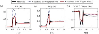
Figure 11. Comparison of lift, drag and aerodynamic torque about pitching axis for Case I without considering the added-mass effect.

Figure 12. Comparison of lift, drag and aerodynamic torque about pitching axis for Case II without considering the added-mass effect.
The calculated and measured results for both cases are shown in figures 11 and 12. For both cases, the lift, drag and torque data from the experiments are plotted in thick lines in black. It should be noted that (i) the drag in this validation is defined in the direction opposite to the translational velocity of the plate while the drag shown in the rest of this paper is defined as the component of aerodynamic force on the
 $y_{i}$
axis in the inertial frame; (ii) the added-mass effect is not considered in the numerical results shown in figures 11 and 12 since the acceleration information during the start and stop phases of pitching motion is unknown. The history of experimentally measured loads can be divided into three phases: (i) before 0.5 s, zero lift and a small amount of drag and torque due to the viscous drag on the plate surface can be found; (ii) from 0.5 to 0.75 s for Case I and to 1 s for Case II, a dramatic increase of loads are reported due to the contribution of the wing rotation and translation; (iii) from 0.75 s for Case I and 1 s for Case II to 2 s, relative steady load histories are shown due to the steady wing sweeping at the stationary AOA. During the first phase, no aerodynamic loads are obtained by the proposed model since the viscous drag is assumed to be negligible. At the beginning of the second phase, the rapid increase trend and the amplitudes are well captured by the proposed analytical model while considering the Wagner effect. In contrast, the loads without the Wagner effect apparently overestimate the peak values. If we compare the loads during the second phase to the loads after the pitching motion stops, it is obvious that the increments of the aerodynamic lift, drag and torque due to the wing rotation are dramatic. When the plate stops pitching up, the magnitudes of the drop of lift and drag are all successfully predicted by the proposed quasi-steady model when considering the Wagner effect. The discrepancy of the aerodynamic torque for both cases can result from the slightly underestimated centre of pressure as shown in figure 8. Based on the comparisons of calculated and measured results for both cases, it can be concluded that the estimations with the Wagner effect show much better agreement to the measurements for all the lift, drag and torque histories and for both cases. This can be explained by the fact that both the Reynolds number (
$y_{i}$
axis in the inertial frame; (ii) the added-mass effect is not considered in the numerical results shown in figures 11 and 12 since the acceleration information during the start and stop phases of pitching motion is unknown. The history of experimentally measured loads can be divided into three phases: (i) before 0.5 s, zero lift and a small amount of drag and torque due to the viscous drag on the plate surface can be found; (ii) from 0.5 to 0.75 s for Case I and to 1 s for Case II, a dramatic increase of loads are reported due to the contribution of the wing rotation and translation; (iii) from 0.75 s for Case I and 1 s for Case II to 2 s, relative steady load histories are shown due to the steady wing sweeping at the stationary AOA. During the first phase, no aerodynamic loads are obtained by the proposed model since the viscous drag is assumed to be negligible. At the beginning of the second phase, the rapid increase trend and the amplitudes are well captured by the proposed analytical model while considering the Wagner effect. In contrast, the loads without the Wagner effect apparently overestimate the peak values. If we compare the loads during the second phase to the loads after the pitching motion stops, it is obvious that the increments of the aerodynamic lift, drag and torque due to the wing rotation are dramatic. When the plate stops pitching up, the magnitudes of the drop of lift and drag are all successfully predicted by the proposed quasi-steady model when considering the Wagner effect. The discrepancy of the aerodynamic torque for both cases can result from the slightly underestimated centre of pressure as shown in figure 8. Based on the comparisons of calculated and measured results for both cases, it can be concluded that the estimations with the Wagner effect show much better agreement to the measurements for all the lift, drag and torque histories and for both cases. This can be explained by the fact that both the Reynolds number (
 $\mathit{Re}=1\times 10^{4}$
) and the kinematics satisfy the conditions where the Wagner effect should be considered.
$\mathit{Re}=1\times 10^{4}$
) and the kinematics satisfy the conditions where the Wagner effect should be considered.

Figure 13. Comparison of unsmoothed and smoothed pitching motion for both cases.
 ${\it\eta}_{1}$
and
${\it\eta}_{1}$
and
 ${\it\eta}_{2}$
are the pitching angles before and after the pitching motion occurring at
${\it\eta}_{2}$
are the pitching angles before and after the pitching motion occurring at
 $t_{1}$
and
$t_{1}$
and
 $t_{2}$
, respectively.
$t_{2}$
, respectively.
The sharp peaks shown in the experimental data at the transitions are attributed to the added-mass effect during the start and stop of the pitching motion (Percin & van Oudheusden Reference Percin and van Oudheusden2015). The pitching motion shown in figure 10 is the ideal case where no transition time is needed to start or stop the pitching motion, which is not true in reality. However, the time required for the brushed DC motor used in the experiment to realize the transition of the wing in water is not clear. In order to quantify the acceleration in transitions, we use a continuously differentiable
 $C^{\infty }$
function (Eldredge, Wang & Ol Reference Eldredge, Wang and Ol2009) to replace the ideal pitching motion, as shown in figure 13. The new function is given by
$C^{\infty }$
function (Eldredge, Wang & Ol Reference Eldredge, Wang and Ol2009) to replace the ideal pitching motion, as shown in figure 13. The new function is given by
 $$\begin{eqnarray}{\it\eta}(t)={\displaystyle \frac{{\it\eta}_{2}-{\it\eta}_{1}}{a(t_{2}-t_{1})}}\ln \left[{\displaystyle \frac{\cosh (a(t-t_{1}))}{\cosh (a(t-t_{2}))}}\right]+{\displaystyle \frac{1}{2}}({\it\eta}_{1}+{\it\eta}_{2}),\end{eqnarray}$$
where
 ${\it\eta}_{1}$
and
${\it\eta}_{1}$
and
 ${\it\eta}_{2}$
are the pitching angles before and after the pitching motion which occur at
${\it\eta}_{2}$
are the pitching angles before and after the pitching motion which occur at
 $t_{1}$
and
$t_{1}$
and
 $t_{2}$
, respectively. The parameter
$t_{2}$
, respectively. The parameter
 $a$
controls the transition time and is set to 40 here to minimize the phase shift between calculated and measured loads. Results obtained from our quasi-steady model including the added-mass effect are also compared with measured data in figures 14 and 15. Apparently, most of the peaks and valleys of the load histories are well captured. The mismatch just before the pitching motion stops might be a result of the imperfection of the hypothetical smoothed pitching motion.
$a$
controls the transition time and is set to 40 here to minimize the phase shift between calculated and measured loads. Results obtained from our quasi-steady model including the added-mass effect are also compared with measured data in figures 14 and 15. Apparently, most of the peaks and valleys of the load histories are well captured. The mismatch just before the pitching motion stops might be a result of the imperfection of the hypothetical smoothed pitching motion.

Figure 14. Comparison of lift, drag and aerodynamic torque about pitching axis for Case I when added-mass effect is considered based on the smoothed pitching motion.

Figure 15. Comparison of lift, drag and aerodynamic torque about pitching axis for Case II when added-mass effect is considered based on the smoothed pitching motion.
3.2 A flapping wing
To further validate the proposed model, we use a flapping wing as another test case which is operated at a much smaller Reynolds number (approximately 100) than that of the sweeping–pitching plate. This experimental measurement was conducted by Whitney & Wood (Reference Whitney and Wood2010) to obtain the passive pitching motion and lift production of an artificial wing which mimics the wing of Eristalis tenax (dronefly).

Figure 16. Wing platform used by Whitney & Wood (Reference Whitney and Wood2010).
As shown in figure 16, the wing span is 15 mm and the spanwise wing area distribution, which can be quantified by the length of all the chordwise strips, is described by the Beta probability density function. The first and second radius of moment of area of the wing are equal to 0.5 and 0.56, respectively, and they are taken as the mean and standard deviation of the beta probability density function. The pitching axis is located at a distance of 0.73 mm from the straight portion of its LE. Due to the variation of the chord length along the span, the normalized local distance between the LE and pitching axis
 $\hat{d}$
changes from the wing root to tip. The wing platform is connected to the drive bar that is located above the wing root with an elastic hinge (polyimide film) of 1.8 mm wide,
$\hat{d}$
changes from the wing root to tip. The wing platform is connected to the drive bar that is located above the wing root with an elastic hinge (polyimide film) of 1.8 mm wide,
 $70~{\rm\mu}\text{m}$
long and
$70~{\rm\mu}\text{m}$
long and
 $7.6~{\rm\mu}\text{m}$
thick.
$7.6~{\rm\mu}\text{m}$
thick.
The passive pitching motion and the net force that consist of both the aerodynamic lift and wing inertia were measured by Whitney & Wood (Reference Whitney and Wood2010). The aerodynamic torque about the pitching axis could not be measured by their set-up directly. Therefore, the capability of our model to estimate the aerodynamic torque has to be validated indirectly by comparing the calculated and measured passive pitching motions. The pitching motion is jointly determined by the hinge stiffness at the wing root, the wing inertia and the aerodynamic torque about the pitching axis. The equation of motion that governs the passive pitching motion is derived in appendix C. The hinge stiffness can be modelled as a linear rotational spring (Howell Reference Howell2001) and the related inertial terms have been measured by Whitney & Wood (Reference Whitney and Wood2010). Consequently, the accuracy of the predicted passive pitching motion mainly depends on how good the aerodynamic torque estimation is.
Two cases of flapping kinematics with different ratios of upstroke-to-downstroke duration (
 $u/d$
),
$u/d$
),
 $u/d=0.79$
for Case I and
$u/d=0.79$
for Case I and
 $u/d=0.62$
for Case II, were studied in the experiments. Rather different passive pitching motions (figures 17 and 18) and lift force histories (figure 21) were reported.
$u/d=0.62$
for Case II, were studied in the experiments. Rather different passive pitching motions (figures 17 and 18) and lift force histories (figure 21) were reported.

Figure 17. Comparison of passive pitching motion between measured and calculated results for Case I. Three calculated results correspond to different combinations of the four terms in our quasi-steady model. ‘
 $d$
’ and ‘
$d$
’ and ‘
 $u$
’ indicate the downstroke and upstroke, respectively.
$u$
’ indicate the downstroke and upstroke, respectively.

Figure 18. Comparison of passive pitching motion between measured and calculated results for Case II. Three calculated results correspond to different combinations of the four terms in our quasi-steady model.
In our simulations, the Wagner effect is not included due to the flapping kinematics and low
 $\mathit{Re}$
, both of which reduce the influence of Wagner effect. The contribution of the small heaving motion is considered. Figures 17 and 18 show the calculated pitching motion when excluding the coupling loads, the rotation-induced loads and using the full model. For both cases, it can be seen that the passive pitching motion predicted by the proposed model that includes all the four loading terms shows best agreement to the experimental data. The inclusion of the rotation-induced loads due to pure wing rotation and the coupling loads between wing translation and rotation improves the prediction of the passive pitching motion by introducing more damping. From the plot of the total aerodynamic torque and its components for both cases as shown in figure 19, it can be clearly seen that (i) the rotation-induced loads and the coupling loads dominate the aerodynamic torque during the wing reversals; and (ii) the coupling between the wing translation and rotation provides additional aerodynamic torque and thus damping on the wing all over a flapping cycle. Although the wing reversals predicted by our model start slightly earlier than that reported by the experimental data, the pitching amplitudes and the phase shift from the sweeping motion (measured from peak-to-peak) are quite close, especially for Case I.
$\mathit{Re}$
, both of which reduce the influence of Wagner effect. The contribution of the small heaving motion is considered. Figures 17 and 18 show the calculated pitching motion when excluding the coupling loads, the rotation-induced loads and using the full model. For both cases, it can be seen that the passive pitching motion predicted by the proposed model that includes all the four loading terms shows best agreement to the experimental data. The inclusion of the rotation-induced loads due to pure wing rotation and the coupling loads between wing translation and rotation improves the prediction of the passive pitching motion by introducing more damping. From the plot of the total aerodynamic torque and its components for both cases as shown in figure 19, it can be clearly seen that (i) the rotation-induced loads and the coupling loads dominate the aerodynamic torque during the wing reversals; and (ii) the coupling between the wing translation and rotation provides additional aerodynamic torque and thus damping on the wing all over a flapping cycle. Although the wing reversals predicted by our model start slightly earlier than that reported by the experimental data, the pitching amplitudes and the phase shift from the sweeping motion (measured from peak-to-peak) are quite close, especially for Case I.

Figure 19. Total aerodynamic torque and its components induced by the wing translation, rotation, the coupling term as well as the added-mass effect for both cases.
Whitney & Wood (Reference Whitney and Wood2010) also compared the predicted passive pitching motion based on their quasi-steady model with the experimental data. As shown by table 1, their model includes the loads resulting from wing translation, pure rotation and the added-mass effect. In their simulation, the translational lift coefficient and rotational damping coefficient were tuned to achieve best agreements with experimental results. They used the CP measured on a dynamically scaled model Drosophila (Dickson et al. Reference Dickson, Straw, Poelma and Dickinson2006) in their simulation. By comparing the passive pitching motion calculated by their quasi-steady model with different combinations of the three components, they argued that the damping due to pure rotation is important but the added-mass effect is not always helpful to reduce the discrepancy with measured results. For Case I, they showed both the calculated passive pitching motion with and without considering the added-mass effect, while for Case II, they only showed the result without considering the added-mass effect. These results are compared with the passive pitching motion predicted by the proposed model in this work as well as the experimental data in figure 20. It can be seen that, without help from any empirical parameters, our quasi-steady model still can give comparable passive pitching motion to the seemingly best results from the model of Whitney & Wood (Reference Whitney and Wood2010) which are based on careful tuning of some parameters. Our model even gives a better prediction of the amplitude of the passive pitching motion.

Figure 20. Comparison of the passive pitching motion predicted by the proposed quasi-steady model and the model of Whitney & Wood (Reference Whitney and Wood2010) for both cases.
The lift force measured by Whitney & Wood (Reference Whitney and Wood2010) is the summation of the aerodynamic and inertial forces of the wing. In figure 21, two types of calculated forces obtained by the proposed model in this work are presented for both cases. One is based on the fully measured kinematics while the other is based on the kinematics with the measured sweeping and heaving motion but calculated passive pitching motion. It is clear to see that with fully measured kinematics our quasi-steady model gives a rather good prediction of the force histories for both cases, except for short periods of overestimation during the upstrokes. The overestimation can be explained by two reasons. First, the shorter duration of upstrokes compared to downstrokes might lead to more complex unsteady flow phenomenon (e.g. Wagner effect) which is a challenge for our quasi-steady model to capture. Second, the angular velocity and acceleration of three Euler angles are calculated based on the corresponding displacements which are fitted from the measured data. This might lead to inaccurate kinematic information, especially the acceleration, which influences the added-mass effect. When the calculated passive pitching motion is used, the overestimation is slightly larger as a result of the discrepancy between calculated and measured pitching motion. But the characteristics of the force histories are still successfully captured, especially during the downstroke.

Figure 21. Comparison of the force histories for both cases between experimental data and calculated results based on both the proposed quasi-steady model and the model from Whitney & Wood (Reference Whitney and Wood2010).
In figure 21, we also show the predicted force history obtained by Whitney & Wood (Reference Whitney and Wood2010). In their simulation, the pure rotation effect is ignored during the force calculation although included in the aerodynamic torque estimation for calculating the passive pitching motion. Even though the careful selection of different terms and tuning of empirical parameters do improve the agreement of lift prediction with measured data, their model is less predictive for arbitrary flapping wings compared to our quasi-steady model which does not rely on any empirical data.
The measured average lift forces are 71.6 mg for Case I and 71.2 mg for Case II, respectively. With the proposed quasi-steady model, the average lift based on the fully measured kinematics is 90.9 mg and 81.6 mg for two cases, respectively. Due to the increase of the discrepancy between measured and calculated pitching motion, the average lift obtained based on the calculated pitching motion is 89.0 mg for Case I and 94.4 mg for Case II. In addition to the error of the predicted passive pitching motion, this overestimated average lift force might be attributed to the fact that the lift is very sensitive to the wing dimensions. For example, if we decrease the wing span by 1 mm while keeping the aspect ratio fixed, the calculated average lift forces based on measured kinematics are reduced to 75.1 and 66.7 mg for the two cases.
Without using any empirical parameters or selectively choosing different terms, our quasi-steady model is still able to give good predictions for the passive pitching motion. Compared to the results obtained by the quasi-steady model proposed by Whitney & Wood (Reference Whitney and Wood2010), the proposed model can give a comparable or slightly better prediction of the passive pitching motion. This implies that our model is more predictive for evaluating the aerodynamic performance of flapping wings in passive pitching motion. Admittedly limited by the inherent drawbacks of the quasi-steady assumption, the unsteady effects, such as the wake capture effect, the Wagner effect and the spatial movement of the LEV on the wing surface, cannot be determined. This might be another reason of the discrepancy of the passive pitching motion and force history between calculated and experimental results.
4 Conclusion
For wings performing translational and rotational motion simultaneously, particularly for flapping wings, we proposed a predictive quasi-steady aerodynamic model. This model is capable of predicting both the aerodynamic force and torque, and it also provides better solutions to three issues which have not been addressed completely by existing quasi-steady models. First is the inconsistency of compositions of existing quasi-steady models, which is eliminated by comprehensively including contributions from wing translation, rotation, their coupling and the added-mass effect in the proposed model. Second is the overall contribution of the wing rotation to the total aerodynamic loads and the corresponding centre of pressure, both of which are required for the estimation of aerodynamic torque. We use two components, including the rotation-induced loads due to the pure wing rotation and the loads due to the coupling between wing rotation and translation, to collaboratively represent the overall contribution of the wing rotation. A new formula for the coupling load has been derived based on the condition that the plate uniformly rotates around its pitching axis in an incoming flow. This condition should be applied as a result of the ‘quasi-steady’ assumption. However, the formula used in most existing quasi-steady models assumes that the plate oscillates around its equilibrium position in a harmonic way. The importance of both components to the quasi-steady model has been shown by the fact that the damping torque excluding the contribution from either of them is far from sufficient to maintain the expected passive pitching motion. The proposed model shows excellent prediction of the centre of pressure of a dynamically scaled Hawkmoth wing conducting translational and rotational motion simultaneously at different angles of attack. Third is that most existing quasi-steady models depend on empirical parameters. In contrast, the proposed model does not rely on any empirical data while it still shows a comparable accuracy on estimating the aerodynamic force, torque and the passive pitching motion as shown by the comparisons with experimental data of two test cases. This implies that the proposed model is more predictive compared to existing quasi-steady models. Therefore, the proposed quasi-steady model can be applied to the design and optimization of flapping wings.
Acknowledgements
The authors would like to acknowledge M. Percin, J. P. Whitney and J. S. Han for providing their experimental data. Thanks are also given to M. Sun, W. B. Tay, H. J. Peters and G. van Lex for useful discussions. The authors would also like to thank the anonymous reviewers for their valuable comments. This work is financially supported by China Scholarship Council (CSC no. 201206290060) and the Atalanta project partly supported by Cooperation DevLab.
Appendix A.
Based on the discretized wing using the BEM, the resultant lift on a rigid flapping wing can be calculated by
 $$\begin{eqnarray}L^{\mathit{trans}}=\int _{0}^{R}\frac{1}{2}{\it\rho}^{f}v^{2}C_{l}^{\mathit{trans}}c\,\text{d}x_{c},\end{eqnarray}$$
where the 2-D lift coefficient
 $C_{l}^{\mathit{trans}}$
is a constant for a given angle of attack. Considering the fact that along the span
$C_{l}^{\mathit{trans}}$
is a constant for a given angle of attack. Considering the fact that along the span
 $v={\it\omega}_{z_{i}}x_{c}$
, the above equation can be rewritten as
$v={\it\omega}_{z_{i}}x_{c}$
, the above equation can be rewritten as
 $$\begin{eqnarray}L^{\mathit{trans}}={\textstyle \frac{1}{2}}{\it\rho}^{f}{\it\omega}_{z_{i}}^{2}R^{2}\hat{r}_{2}^{2}C_{l}^{\mathit{trans}}S,\end{eqnarray}$$
where
 $S$
is the wing area (
$S$
is the wing area (
 $=\int _{0}^{R}c\,\text{d}x_{c}$
) and
$=\int _{0}^{R}c\,\text{d}x_{c}$
) and
 $\hat{r}_{2}$
is the span-normalized distance from the root chord to the gyradius which is given by
$\hat{r}_{2}$
is the span-normalized distance from the root chord to the gyradius which is given by
 $$\begin{eqnarray}\hat{r}_{2}=\sqrt{\frac{1}{SR^{2}}\int _{0}^{R}x_{c}^{2}c\,\text{d}x_{c}}.\end{eqnarray}$$
When the translation velocity at the gyradius is taken as the reference velocity, the lift force based on the 3-D lift coefficient
 $C_{L}^{\mathit{trans}}$
can be written as
$C_{L}^{\mathit{trans}}$
can be written as
 $$\begin{eqnarray}L^{\mathit{trans}}={\textstyle \frac{1}{2}}{\it\rho}^{f}(\hat{r}_{2}R{\it\omega}_{z_{i}})^{2}C_{L}^{\mathit{trans}}S.\end{eqnarray}$$
By comparing equations (A 2) and (A 4), it can be seen found that
 $C_{L}^{\mathit{trans}}$
can be used directly as the 2-D lift coefficient
$C_{L}^{\mathit{trans}}$
can be used directly as the 2-D lift coefficient
 $C_{l}^{\mathit{trans}}$
for the BEM as long as the reference velocity is at gyration.
$C_{l}^{\mathit{trans}}$
for the BEM as long as the reference velocity is at gyration.
Appendix B.
To derive the loads experienced by a plate uniformly rotating around its pitching axis at zero AOA when immersed in an incoming flow with a velocity of
 $v_{z_{c}}$
, the acceleration potential method is used (Fung Reference Fung1993). Assuming that the rotational angle is infinitesimal and the velocity of the incoming flow is much higher than the rotational velocity, the horizontal offset of the plate due to the rotation is negligible. Setting the time with respect to zero AOA to be
$v_{z_{c}}$
, the acceleration potential method is used (Fung Reference Fung1993). Assuming that the rotational angle is infinitesimal and the velocity of the incoming flow is much higher than the rotational velocity, the horizontal offset of the plate due to the rotation is negligible. Setting the time with respect to zero AOA to be
 $t=0$
, the plate position can be described as a function of time
$t=0$
, the plate position can be described as a function of time
 $$\begin{eqnarray}y_{w}={\it\omega}_{x_{c}}t\left(x_{w}+c\hat{d}-\frac{c}{2}\right),\quad -\frac{c}{2}\leqslant x_{w}\leqslant \frac{c}{2},\end{eqnarray}$$
where
 $x_{w}$
and
$x_{w}$
and
 $y_{w}$
are axes of the introduced frame as shown in figure 22.
$y_{w}$
are axes of the introduced frame as shown in figure 22.

Figure 22. Illustration of a plate uniformly rotating around its pitching axis within an infinitesimal time interval
 $t_{1}$
when immersed horizontally in an incoming flow at velocity of
$t_{1}$
when immersed horizontally in an incoming flow at velocity of
 $v_{z_{c}}$
.
$v_{z_{c}}$
.
The fluid surrounding the plate needs to satisfy three boundary conditions (BCs): (i) the flow on its surface must be tangent to the plate both in the velocity and acceleration field; (ii) the Kutta condition has to be satisfied at the TE; (iii) the fluid acceleration at infinity should be zero. For inviscid and incompressible flow, the momentum equation can be written as
 $$\begin{eqnarray}\boldsymbol{a}^{f}=\boldsymbol{{\rm\nabla}}({\rm\Phi}),\end{eqnarray}$$
where
 $\boldsymbol{a}^{f}$
represents the fluid acceleration and
$\boldsymbol{a}^{f}$
represents the fluid acceleration and
 ${\rm\Phi}$
is the acceleration potential which is equal to
${\rm\Phi}$
is the acceleration potential which is equal to
 $-p/{\it\rho}^{f}$
. This implies that the static pressure
$-p/{\it\rho}^{f}$
. This implies that the static pressure
 $p$
is proportional to the acceleration potential
$p$
is proportional to the acceleration potential
 ${\rm\Phi}$
. Meanwhile, there exists a conjugate function
${\rm\Phi}$
. Meanwhile, there exists a conjugate function
 ${\rm\Psi}$
orthogonal to
${\rm\Psi}$
orthogonal to
 ${\rm\Phi}$
and satisfying
${\rm\Phi}$
and satisfying
 $$\begin{eqnarray}\frac{\partial {\rm\Phi}}{\partial x_{w}}=\frac{\partial {\rm\Psi}}{\partial y_{w}}=v_{x_{w}},\quad \frac{\partial {\rm\Phi}}{\partial y_{w}}=-\frac{\partial {\rm\Psi}}{\partial x_{w}}=v_{y_{w}}.\end{eqnarray}$$
Then, a complex acceleration potential
 $W$
can be constructed as
$W$
can be constructed as
 $$\begin{eqnarray}W(z)={\rm\Phi}+j{\rm\Psi},\end{eqnarray}$$
where
 $z$
is a complex variable (i.e.
$z$
is a complex variable (i.e.
 $z=x_{w}+jy_{w}$
) on the complex plane. Instead of searching for a value of
$z=x_{w}+jy_{w}$
) on the complex plane. Instead of searching for a value of
 ${\rm\Phi}$
that satisfies all the BCs, it is easier to construct the corresponding complex acceleration potential
${\rm\Phi}$
that satisfies all the BCs, it is easier to construct the corresponding complex acceleration potential
 $W$
. According to the linearized theory, for a plate at infinitesimal AOA, BCs can be applied to the projection of the plate on the
$W$
. According to the linearized theory, for a plate at infinitesimal AOA, BCs can be applied to the projection of the plate on the
 $x_{w}$
axis. The plate on the initial complex plane is mapped to a circle on the
$x_{w}$
axis. The plate on the initial complex plane is mapped to a circle on the
 ${\it\zeta}$
complex plane with conformal transformation
${\it\zeta}$
complex plane with conformal transformation
 $$\begin{eqnarray}z=\frac{1}{2}\left({\it\zeta}+\frac{c^{2}}{4{\it\zeta}}\right).\end{eqnarray}$$
On the
 ${\it\zeta}$
plane, the flow field described by the following complex acceleration potential
${\it\zeta}$
plane, the flow field described by the following complex acceleration potential
 $$\begin{eqnarray}W({\it\zeta})=\frac{jA_{0}}{{\it\zeta}-c/2}+\frac{jA_{1}}{{\it\zeta}}\end{eqnarray}$$
has the potential to satisfy all three BCs. Firstly, it is continuous at the TE, which means that the Kutta condition is satisfied. Secondly,
 $W({\it\zeta})$
tends to be zero at infinity which implies that the acceleration also tends to zero. Therefore, the flow field automatically satisfies the BC at infinity. Thirdly, the coefficients
$W({\it\zeta})$
tends to be zero at infinity which implies that the acceleration also tends to zero. Therefore, the flow field automatically satisfies the BC at infinity. Thirdly, the coefficients
 $A_{0}$
and
$A_{0}$
and
 $A_{1}$
can be determined by applying the velocity and acceleration BCs on the plate surface. Their boundary values are
$A_{1}$
can be determined by applying the velocity and acceleration BCs on the plate surface. Their boundary values are
 $$\begin{eqnarray}\displaystyle & \displaystyle v_{y_{w}}=\frac{\text{D}y_{w}}{\text{D}t}=-v_{z_{c}}{\it\omega}_{x_{c}}t+{\it\omega}_{x_{c}}\left(x_{w}+c\hat{d}-\frac{c}{2}\right), & \displaystyle\end{eqnarray}$$
 $$\begin{eqnarray}\displaystyle & \displaystyle a_{y_{w}}=\frac{\text{D}^{2}y_{w}}{\text{D}t^{2}}=-2v_{z_{c}}{\it\omega}_{x_{c}}. & \displaystyle\end{eqnarray}$$
The normal component of the fluid acceleration on the circle (
 ${\it\zeta}$
plane) can be calculated by
${\it\zeta}$
plane) can be calculated by
 $$\begin{eqnarray}a_{r}^{f}|_{|{\it\zeta}|=c/2}=\left.\frac{\partial \mathit{Re}(W)}{\partial r}\right|_{|{\it\zeta}|=c/2}=-\frac{4}{c^{2}}A_{1}\sin {\it\gamma},\end{eqnarray}$$
where
 $r$
(
$r$
(
 $r=c/2$
on the circle) and
$r=c/2$
on the circle) and
 ${\it\gamma}$
are polar coordinates on the
${\it\gamma}$
are polar coordinates on the
 ${\it\zeta}$
plane.
${\it\zeta}$
plane.
 $a_{r}^{f}|_{|{\it\zeta}|=c/2}$
should be equal to
$a_{r}^{f}|_{|{\it\zeta}|=c/2}$
should be equal to
 $a_{y_{w}}\sin {\it\gamma}$
in order to satisfy the acceleration BC on the plate surface, whereby the coefficient
$a_{y_{w}}\sin {\it\gamma}$
in order to satisfy the acceleration BC on the plate surface, whereby the coefficient
 $A_{1}$
is obtained as
$A_{1}$
is obtained as
 $$\begin{eqnarray}A_{1}={\textstyle \frac{1}{2}}v_{z_{c}}{\it\omega}_{x_{c}}c^{2}.\end{eqnarray}$$
The velocity BC can be used to calculate the coefficient
 $A_{0}$
. The fluid velocity
$A_{0}$
. The fluid velocity
 $v_{y_{w}}^{f}$
on the plate in the
$v_{y_{w}}^{f}$
on the plate in the
 ${\it\zeta}$
plane can be calculated by solving the partial differentiation equation
${\it\zeta}$
plane can be calculated by solving the partial differentiation equation
 $$\begin{eqnarray}\frac{\partial v_{y_{w}}^{f}}{\partial t}-v_{z_{c}}\frac{\partial v_{y_{w}}^{f}}{\partial x_{w}}=a_{y_{w}}^{f}=-\frac{\partial {\rm\Psi}}{\partial x_{w}}.\end{eqnarray}$$
The fluid velocity on the plate can be obtained as
 $$\begin{eqnarray}v_{y_{w}}^{f}=\frac{{\rm\Psi}}{v_{z_{c}}}+h(v_{z_{c}}t+x_{w}),\end{eqnarray}$$
where
 $h(\cdot )$
can be an arbitrary function of the expression
$h(\cdot )$
can be an arbitrary function of the expression
 $v_{z_{c}}t+x_{w}$
and
$v_{z_{c}}t+x_{w}$
and
 ${\rm\Psi}$
is equal to
${\rm\Psi}$
is equal to
 $2v_{z_{c}}{\it\omega}_{x_{c}}x_{w}-A_{0}/c$
which is obtained from (B 6) by substituting
$2v_{z_{c}}{\it\omega}_{x_{c}}x_{w}-A_{0}/c$
which is obtained from (B 6) by substituting
 ${\it\zeta}$
with
${\it\zeta}$
with
 $z$
which is determined by
$z$
which is determined by
 $x_{w}$
and
$x_{w}$
and
 $y_{w}$
. If we let
$y_{w}$
. If we let
 $h(v_{z_{c}}t+x_{w})$
be
$h(v_{z_{c}}t+x_{w})$
be
 $-{\it\omega}(v_{z_{c}}t+x_{w})$
and apply the velocity BC that the fluid velocity
$-{\it\omega}(v_{z_{c}}t+x_{w})$
and apply the velocity BC that the fluid velocity
 $v_{y_{w}}^{f}$
is equal to the boundary value of the velocity given in (B 7) over the plate, except for the singular point at the LE, we obtain
$v_{y_{w}}^{f}$
is equal to the boundary value of the velocity given in (B 7) over the plate, except for the singular point at the LE, we obtain
 $$\begin{eqnarray}A_{0}=v_{z_{c}}{\it\omega}_{x_{c}}c^{2}({\textstyle \frac{1}{2}}-\hat{d}).\end{eqnarray}$$
Substituting equations (B 10) and (B 13) into (B 6), the acceleration potential
 ${\rm\Phi}$
can be obtained as
${\rm\Phi}$
can be obtained as
 $$\begin{eqnarray}{\rm\Phi}=v_{z_{c}}{\it\omega}_{x_{c}}c\sin ({\it\gamma})-\frac{2v_{z_{c}}{\it\omega}_{x_{c}}\sin ({\it\gamma})c(\hat{d}-\frac{1}{2})}{(1-\cos ({\it\gamma}))^{2}+\sin ^{2}({\it\gamma})},\end{eqnarray}$$
with which the pressure distribution can be calculated. Eventually, the lift
 $L$
and torque
$L$
and torque
 ${\it\tau}$
about the pitching axis due to the coupling effect on a plate with unity span can be obtained by integrating the pressure over the entire circle on the
${\it\tau}$
about the pitching axis due to the coupling effect on a plate with unity span can be obtained by integrating the pressure over the entire circle on the
 ${\it\zeta}$
plane, resulting in,
${\it\zeta}$
plane, resulting in,
 $$\begin{eqnarray}\displaystyle & \displaystyle L={\rm\pi}{\it\rho}^{f}v_{z_{c}}{\it\omega}_{x_{c}}c^{2}({\textstyle \frac{3}{4}}-\hat{d})+{\textstyle \frac{1}{4}}{\rm\pi}{\it\rho}v_{z_{c}}{\it\omega}_{x_{c}}c^{2}, & \displaystyle\end{eqnarray}$$
 $$\begin{eqnarray}\displaystyle & \displaystyle {\it\tau}={\rm\pi}{\it\rho}^{f}v_{z_{c}}{\it\omega}_{x_{c}}c^{3}({\textstyle \frac{3}{4}}-\hat{d})({\textstyle \frac{1}{4}}-\hat{d})+{\textstyle \frac{1}{4}}{\rm\pi}{\it\rho}v_{z_{c}}{\it\omega}_{x_{c}}c^{3}({\textstyle \frac{3}{4}}-\hat{d}), & \displaystyle\end{eqnarray}$$
 ${\rm\pi}{\it\rho}^{f}c^{2}/4$
while flowing on a rotating wing. It should be noted that
${\rm\pi}{\it\rho}^{f}c^{2}/4$
while flowing on a rotating wing. It should be noted that
 ${\it\tau}$
is, by convention, considered to be positive when it acts to pitch the plate in the nose-up direction.
${\it\tau}$
is, by convention, considered to be positive when it acts to pitch the plate in the nose-up direction.
Appendix C.
In this appendix, the equation of motion that governs the passive pitching motion of flapping wings is derived.
Generally, the passive pitching motion is achieved by connecting the wing to the drive mechanism with an elastic hinge while the drive mechanism applies a sweeping torque. Then, the wing is forced to pitch about the pitching axis by the wing inertia and aerodynamic loads. Since the out-of-plane motion is not completely constrained, a slight heaving motion might be observed, as shown in the second validation case. Indeed, the heaving motion makes a small contribution to the drive torque and the passive pitching motion. The contribution of gravity to the passive pitching motion is ignored due to the small wing mass and the fact that the centre of mass is not far away from the pitching axis.
Since the moment of inertia
 $\unicode[STIX]{x1D644}$
of the wing is constant in the co-rotating frame, Euler’s second law of motion for a rigid body is applied about the pitching axis of the wing (i.e.
$\unicode[STIX]{x1D644}$
of the wing is constant in the co-rotating frame, Euler’s second law of motion for a rigid body is applied about the pitching axis of the wing (i.e.
 $x_{c}$
axis), namely,
$x_{c}$
axis), namely,
 $$\begin{eqnarray}{\it\tau}_{x_{c}}^{\mathit{ applied}}+{\it\tau}_{x_{c}}^{\mathit{ iner}}=0,\end{eqnarray}$$
where
 ${\it\tau}_{x_{c}}^{\mathit{applied}}$
consists of the elastic torque
${\it\tau}_{x_{c}}^{\mathit{applied}}$
consists of the elastic torque
 ${\it\tau}_{x_{c}}^{\mathit{elas}}$
(
${\it\tau}_{x_{c}}^{\mathit{elas}}$
(
 $=-k_{{\it\eta}}{\it\eta}$
) from the hinge and the aerodynamic torque
$=-k_{{\it\eta}}{\it\eta}$
) from the hinge and the aerodynamic torque
 ${\it\tau}_{x_{c}}^{\mathit{aero}}$
which includes the four parts as presented in § 2.2. The inertial torque in the co-rotating frame can be calculated by
${\it\tau}_{x_{c}}^{\mathit{aero}}$
which includes the four parts as presented in § 2.2. The inertial torque in the co-rotating frame can be calculated by
 $$\begin{eqnarray}{\bf\tau}^{\mathit{iner}}=-\unicode[STIX]{x1D644}{\bf\alpha}_{c}-{\bf\omega}_{c}\times (\unicode[STIX]{x1D644}{\bf\omega}_{c}),\end{eqnarray}$$
where
 ${\bf\omega}_{c}$
and
${\bf\omega}_{c}$
and
 ${\bf\alpha}_{c}$
are the angular velocity and acceleration in the co-rotating frame and the two components are the torque due to Euler and Coriolis forces, respectively. The component of
${\bf\alpha}_{c}$
are the angular velocity and acceleration in the co-rotating frame and the two components are the torque due to Euler and Coriolis forces, respectively. The component of
 ${\bf\tau}^{\mathit{iner}}$
on the
${\bf\tau}^{\mathit{iner}}$
on the
 $x_{c}$
axis can be divided into the term
$x_{c}$
axis can be divided into the term
 $-I_{x_{c}x_{c}}\ddot{{\it\eta}}$
and the inertial drive torque
$-I_{x_{c}x_{c}}\ddot{{\it\eta}}$
and the inertial drive torque
 ${\it\tau}_{x_{c}}^{\mathit{drive}}$
which can be expressed as
${\it\tau}_{x_{c}}^{\mathit{drive}}$
which can be expressed as
 $$\begin{eqnarray}\displaystyle {\it\tau}_{x_{c}}^{\mathit{drive}} & = & \displaystyle I_{x_{c}x_{c}}\left[{\textstyle \frac{1}{2}}\dot{{\it\phi}}^{2}\cos ^{2}{\it\theta}\sin (2{\it\eta})-{\textstyle \frac{1}{2}}\dot{{\it\theta}}^{2}\sin (2{\it\eta})+2\dot{{\it\phi}}\dot{{\it\theta}}\cos {\it\theta}\cos ^{2}{\it\eta}+\ddot{{\it\phi}}\sin {\it\theta}\right]\nonumber\\ \displaystyle & & \displaystyle +\,I_{x_{c}z_{c}}\left[\ddot{{\it\theta}}\sin {\it\eta}+{\textstyle \frac{1}{2}}\dot{{\it\phi}}^{2}\sin (2{\it\theta})\sin {\it\eta}-\ddot{{\it\phi}}\cos {\it\theta}\cos {\it\eta}+2\dot{{\it\phi}}\dot{{\it\theta}}\sin {\it\theta}\cos {\it\eta}\right].\qquad\end{eqnarray}$$
Eventually, the equation of motion of the wing pitching can be expressed as
 $$\begin{eqnarray}I_{x_{c}x_{c}}\ddot{{\it\eta}}+k_{{\it\eta}}{\it\eta}={\it\tau}_{x_{c}}^{\mathit{ aero}}+{\it\tau}_{x_{c}}^{\mathit{ drive}}.\end{eqnarray}$$


