


1 Introduction
The development of reduced-order models (ROMs) to represent the physics of fluid flows is a subject of considerable current interest in fluid mechanics. The construction of such models is motivated e.g. by potential applications to flow control for drag reduction and noise suppression (Brunton & Noack Reference Brunton and Noack2015). Spatial shapes that serve as the bases for ROMs can be classified as mathematical, empirical or physical modes. Mathematical modes form a complete basis by definition, and many ROMs based on expansion functions have been used for simple boundary conditions (Busse Reference Busse1991; Noack & Eckelmann Reference Noack and Eckelmann1994). Empirical ROMs such as the proper orthogonal decomposition (POD, Berkooz, Holmes & Lumley Reference Berkooz, Holmes and Lumley1993) or the dynamic mode decomposition (DMD, Schmid Reference Schmid2010) arise from postprocessing of numerical or experimental flow data. The present work expounds a novel ROM based on physical modes emergent from the Navier–Stokes equations.
Noack, Morzynski & Tadmor (Reference Noack, Morzynski and Tadmor2011) proposed that linear global stability analysis could be employed to obtain physical modes associated with linear dynamics from the Navier–Stokes equations. Such analyses are based on a decomposition of the flow into a steady or periodic laminar base flow and an infinitesimal perturbation that develops in time, leading to an eigenvalue problem whose eigenvalues characterize the stability of the base flow. The eigenmodes can be employed as spatial shapes to construct ROMs. While computationally demanding if the base flow is three-dimensional, spatially complicated, or the Reynolds number is large, methodologies for numerical linear global stability analyses are becoming mature.
A different type of challenge arises from the application of global stability analysis to turbulent or, more generally, to nonlinear flows. By nonlinear flows, we mean unsteady flows in which there exist different frequencies that interact with each other; feedback via the nonlinear terms in the Navier–Stokes equations is relevant. The key step enabling global stability analysis of nonlinear flows is to consider the time-mean flow as the base flow. Barkley (Reference Barkley2006) applied global stability analysis to the wake of a circular cylinder to study the shedding frequency at Reynolds numbers above the onset of vortex shedding. It was observed that linear stability analysis of unstable (symmetric) steady base flows provided frequencies and global modes different from those observed in numerical simulations and experiments. However, when applied to the mean flow, the method was able to predict frequencies and flow structures similar to those observed in numerical simulations and experiments. More recently, Oberleithner, Rukes & Soria (Reference Oberleithner, Rukes and Soria2014) applied the same methodology to jets. Despite apparent successes of the method in these cases, global stability analysis applied to mean flows can be considered dubious for two reasons.
The first reason is that time-averaged flows are not solutions of the Navier–Stokes equations, but of the Reynolds-averaged Navier–Stokes (RANS) equations. The closure problem is thus inherent in the approach and the unknown Reynolds stress, arising from the interaction of turbulent fluctuations with the mean, must be considered. One way to avoid this issue for weakly nonlinear flows is to employ the assumption, proposed by Barkley (Reference Barkley2006), that the forcing generated by the fluctuations is steady; it only contributes as Reynolds stress in the mean-flow equation. Another approach is to close the RANS equations via the Boussinesq hypothesis and employ an Newtonian eddy viscosity to account for the Reynolds stress. However, this applies only for fully developed turbulent flows in which the diffusion induced by the turbulence can be approximated by an additional eddy viscosity. This approach was introduced in conjunction with a triple decomposition by Hussain & Reynolds (Reference Hussain and Reynolds1970) in order to identify coherent flow structures in turbulent shear flows, and more recently employed e.g. by Meliga, Pujals & Serre (Reference Meliga, Pujals and Serre2012) in an flow control context. To our knowledge, no existing method is able to account for nonlinearity in flows which are neither weakly nonlinear nor fully turbulent.
The second concern with mean-flow stability analysis is with its reliability. Sipp & Lebedev (Reference Sipp and Lebedev2007) replicated Barkley’s work on the cylinder mean flow, then applied the same methodology to an open cavity flow. In the latter case, the predicted frequencies did not match those observed in direct numerical simulation (DNS) and attributed the discrepancy to the relative strength of the mean flow and harmonics, linked to the non-normality of the flow, such that the global modes obtained are non-orthogonal. This is not a desirable characteristic when choosing a ROM, since the projection of flow solutions onto global modes would be ill-conditioned, as discussed by Cerqueira & Sipp (Reference Cerqueira and Sipp2014).
In the following we show that the resolvent analysis for turbulent flows developed by McKeon & Sharma (Reference Mckeon and Sharma2010) represents an alternative strategy to identify physical flow structures in nonlinear flows. The methodology consists of an amplification analysis of the Navier–Stokes equations in the frequency domain, yielding a linear relationship between the velocity field at specific wavenumbers and the nonlinear interaction between other wavenumbers via a resolvent operator. A singular value decomposition (SVD) of the operator reveals that it acts as a very selective directional amplifier of the nonlinear terms, and hence a low-rank approximation of the resolvent is able to reproduce the dominant features of the flow. The time-mean flow must be given as input.
Resolvent analyses have been successfully employed to qualitatively describe the behaviour of flow structures in turbulent canonical flows (Sharma & McKeon Reference Sharma and Mckeon2013) and to identify sparsity effects in direct numerical simulation with periodic finite-length domain (Gómez et al. Reference Gómez, Blackburn, Rudman, Mckeon, Luhar, Moarref and Sharma2014). The technique has also been applied to model scalings in turbulent flows (Moarref et al. Reference Moarref, Sharma, Tropp and Mckeon2013) and to wall-based closed-loop flow control strategies (Luhar, Sharma & McKeon Reference Luhar, Sharma and Mckeon2014, Reference Luhar, Sharma and Mckeon2015). We will explain how the analysis circumvents the above-mentioned limitations of the mean-flow global stability analysis in a ROM context. As an example, we demonstrate the potential of this methodology by employing a two-dimensional resolvent formulation (Åkervik et al. Reference Åkervik, Ehrenstein, Gallaire and Henningson2008; Brandt et al. Reference Brandt, Sipp, Pralits and Marquet2011; Gómez et al. Reference Gómez, Blackburn, Rudman, Mckeon, Luhar, Moarref and Sharma2014) to obtain the relevant flow features in a three-dimensional spanwise-periodic lid-driven cavity flow. For this purpose, a ROM is derived by employing the mean flow and minimal temporal and spatial spectral information.
Lid-driven cavity flows can possess complex features despite the simple geometry, hence they serve as a model problem for many engineering applications dealing with flow recirculation. From the work of Koseff & Street (Reference Koseff and Street1984), it is known that most of the velocity fluctuation in the lid-driven cavity is caused by Taylor–Görtler-like (TGL) vortices. The naming of these vortices is justified by resemblances of the two-dimensional base flow and the corresponding three-dimensional features with the respective flows in the Taylor and Görtler problems, as discussed by Albensoeder & Kuhlmann (Reference Albensoeder and Kuhlmann2006) in their study of the nonlinear stability boundaries of the flow. Depending on the spanwise length and Reynolds number, different numbers of TGL pairs of vortices can coexist in the flow. In the following, we select flow conditions such that the flow possesses structures with distinct associated frequencies that interact, but is far from a turbulent state. Resolvent analysis is be employed to construct a reduced-order model of this type of flow.
2 Description of the flow
The spanwise-periodic lid-driven cavity flow with a square cross-section is governed by the three-dimensional incompressible Navier–Stokes equations
 $$\begin{eqnarray}\partial _{t}\hat{\boldsymbol{u}}+\hat{\boldsymbol{u}}\boldsymbol{\cdot }\boldsymbol{{\rm\nabla}}\hat{\boldsymbol{u}}=-\boldsymbol{{\rm\nabla}}\hat{p}+\mathit{Re}^{-1}{\rm\nabla}^{2}\hat{\boldsymbol{u}},\quad \boldsymbol{{\rm\nabla}}\boldsymbol{\cdot }\hat{\boldsymbol{u}}=0,\end{eqnarray}$$
where
 $\mathit{Re}$
is the Reynolds number based on the steady lid speed
$\mathit{Re}$
is the Reynolds number based on the steady lid speed
 $U$
and cavity depth
$U$
and cavity depth
 $D$
,
$D$
,
 $\hat{\boldsymbol{u}}=(u,v,w)$
is the velocity vector expressed in Cartesian coordinates
$\hat{\boldsymbol{u}}=(u,v,w)$
is the velocity vector expressed in Cartesian coordinates
 $(x,y,z)$
and
$(x,y,z)$
and
 $\hat{p}$
is the modified pressure. The geometry is illustrated in figure 1(a), in which
$\hat{p}$
is the modified pressure. The geometry is illustrated in figure 1(a), in which
 ${\it\Lambda}/D$
denotes the periodic span of the cavity. No-slip boundary conditions are imposed at the walls.
${\it\Lambda}/D$
denotes the periodic span of the cavity. No-slip boundary conditions are imposed at the walls.
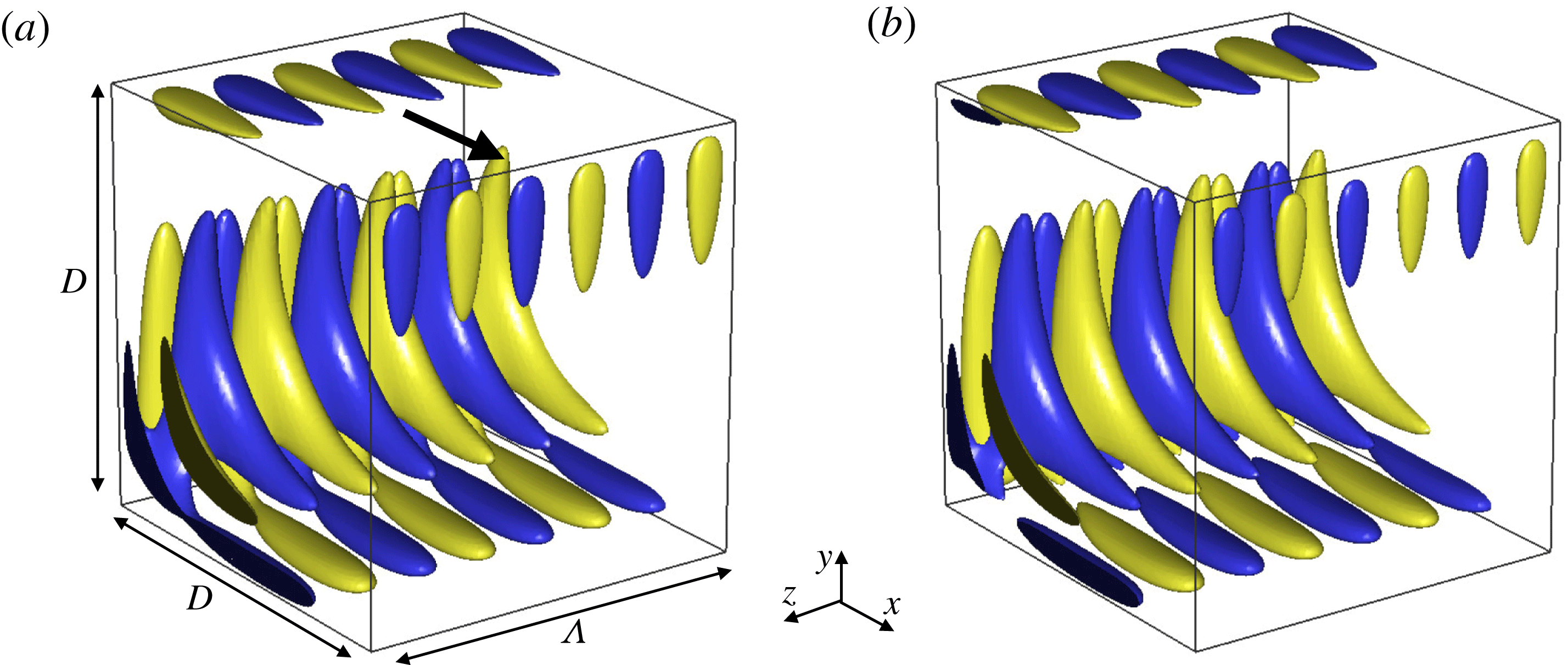
Figure 1. Representation of TGL vortices in the lid-driven cavity flow at
 $\mathit{Re}=1200$
and
$\mathit{Re}=1200$
and
 ${\it\Lambda}/D=0.945$
; lid moves in the direction of arrow. Snapshot of isosurfaces of 20 % max/min spanwise velocity of spanwise Fourier mode
${\it\Lambda}/D=0.945$
; lid moves in the direction of arrow. Snapshot of isosurfaces of 20 % max/min spanwise velocity of spanwise Fourier mode
 ${\it\beta}=3$
. (a) DNS, (b) resolvent-based model. Animations of isosurfaces of DNS and model are shown in supplementary movies 1 and 2 respectively, available at http://dx.doi.org/10.1017/jfm.2016.339.
${\it\beta}=3$
. (a) DNS, (b) resolvent-based model. Animations of isosurfaces of DNS and model are shown in supplementary movies 1 and 2 respectively, available at http://dx.doi.org/10.1017/jfm.2016.339.
DNS of the incompressible lid-driven cavity flow has been carried out using a spectral element–Fourier solver (Blackburn & Sherwin Reference Blackburn and Sherwin2004). Nodal elemental basis functions are used in the
 $(x,y)$
plane while a Fourier expansion basis is employed in the homogeneous direction
$(x,y)$
plane while a Fourier expansion basis is employed in the homogeneous direction
 $(z)$
. The flow solution can be written as a sum of spanwise Fourier modes
$(z)$
. The flow solution can be written as a sum of spanwise Fourier modes
 $$\begin{eqnarray}\hat{\boldsymbol{u}}(x,y,z,t)=\mathop{\sum }_{{\it\beta}}\boldsymbol{u}_{{\it\beta}}(x,y,t)\text{e}^{\text{i}{\it\beta}z}+\text{c.c.},\end{eqnarray}$$
with
 ${\it\beta}$
a non-dimensional spanwise wavenumber normalized with the span
${\it\beta}$
a non-dimensional spanwise wavenumber normalized with the span
 ${\it\Lambda}$
. Based on the nonlinear stability boundaries investigated by Albensoeder & Kuhlmann (Reference Albensoeder and Kuhlmann2006), we chose parameters
${\it\Lambda}$
. Based on the nonlinear stability boundaries investigated by Albensoeder & Kuhlmann (Reference Albensoeder and Kuhlmann2006), we chose parameters
 $\mathit{Re}=1200$
and
$\mathit{Re}=1200$
and
 ${\it\Lambda}/D=0.945$
for our simulations. This selection provides an unsteady flow with multiple frequencies and three pairs of TGL vortices. Figure 1(a) represents the spanwise velocity isosurfaces of the flow and three pairs of vortices may be identified. The temporal behaviour of these vortices is shown in supplementary movie 1, which presents animations of spanwise velocity isosurfaces.
${\it\Lambda}/D=0.945$
for our simulations. This selection provides an unsteady flow with multiple frequencies and three pairs of TGL vortices. Figure 1(a) represents the spanwise velocity isosurfaces of the flow and three pairs of vortices may be identified. The temporal behaviour of these vortices is shown in supplementary movie 1, which presents animations of spanwise velocity isosurfaces.
Figure 2 presents the temporal evolution of the kinetic energy based on (2.2) of the energetically relevant spanwise Fourier modes. This measure indicates when the flow reaches a statistically steady periodic state. Data for
 $t<300$
have been discarded and flow statistics collected until those for the mean flow converged. This two-dimensional flow is the basis of our subsequent resolvent analysis. Mode
$t<300$
have been discarded and flow statistics collected until those for the mean flow converged. This two-dimensional flow is the basis of our subsequent resolvent analysis. Mode
 ${\it\beta}=0$
contains the mean flow while
${\it\beta}=0$
contains the mean flow while
 ${\it\beta}=3$
consist of three pairs of TGL vortices. Self-interaction of mode
${\it\beta}=3$
consist of three pairs of TGL vortices. Self-interaction of mode
 ${\it\beta}=3$
provides energy to its harmonics, but the energy associated with these modes is an order of magnitude smaller.
${\it\beta}=3$
provides energy to its harmonics, but the energy associated with these modes is an order of magnitude smaller.
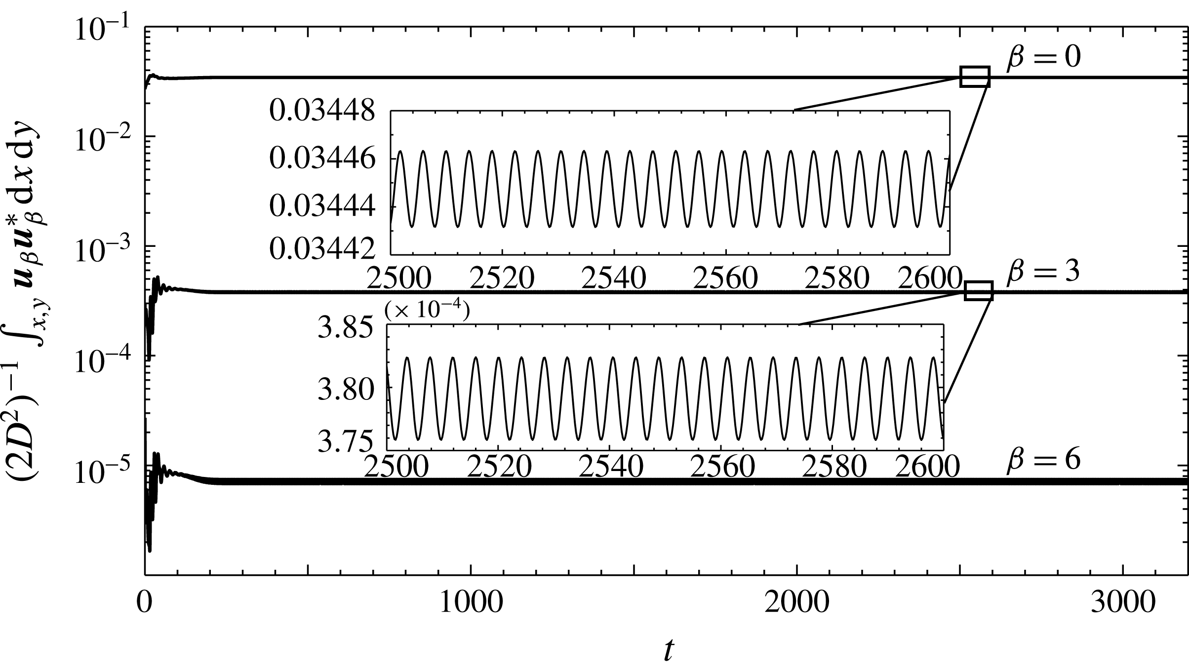
Figure 2. Temporal evolution of the kinetic energy based on (2.2) of the three most energetic spanwise Fourier modes. Mode
 ${\it\beta}=0$
contains the mean flow while
${\it\beta}=0$
contains the mean flow while
 ${\it\beta}=3$
consists of three pairs of TGL vortices. Self-interaction of mode
${\it\beta}=3$
consists of three pairs of TGL vortices. Self-interaction of mode
 ${\it\beta}=3$
provides energy to its harmonic
${\it\beta}=3$
provides energy to its harmonic
 ${\it\beta}=6$
.
${\it\beta}=6$
.
Spatial resolution convergence is achieved with a mesh consisting of 132 spectral elements with polynomial degree
 $N_{p}=9$
in each of the
$N_{p}=9$
in each of the
 $(x,y)$
planes and 64 spanwise Fourier modes. 500 time steps are employed to integrate a time unit
$(x,y)$
planes and 64 spanwise Fourier modes. 500 time steps are employed to integrate a time unit
 $D/U$
.
$D/U$
.
3 Description of the model
3.1 Resolvent analysis
Here we extend the resolvent analysis of McKeon & Sharma (Reference Mckeon and Sharma2010) for pipe flows to the spanwise-periodic three-dimensional lid-driven cavity flow under consideration. The flow is assumed to be statistically steady. A spanwise and time-averaged mean flow
 $\boldsymbol{u}_{0,0}$
is obtained from the DNS and subtracted from the total velocity to leave the fluctuating velocity
$\boldsymbol{u}_{0,0}$
is obtained from the DNS and subtracted from the total velocity to leave the fluctuating velocity
 $\boldsymbol{u}=\hat{\boldsymbol{u}}-\boldsymbol{u}_{0,0}$
, which may be decomposed as a sum of Fourier mode in spanwise direction and time
$\boldsymbol{u}=\hat{\boldsymbol{u}}-\boldsymbol{u}_{0,0}$
, which may be decomposed as a sum of Fourier mode in spanwise direction and time
 $$\begin{eqnarray}\boldsymbol{u}(x,y,z,t)=\mathop{\sum }_{{\it\beta}}\mathop{\sum }_{{\it\omega}}\boldsymbol{u}_{{\it\beta},{\it\omega}}(x,y)\text{e}^{\text{i}({\it\beta}z-{\it\omega}t)}+\text{c.c.}\end{eqnarray}$$
Both
 ${\it\beta}$
and
${\it\beta}$
and
 ${\it\omega}$
are real, and the continuous integral in frequency has been expressed as a sum for simplicity. A similar decomposition may be applied to the nonlinear terms, leading to
${\it\omega}$
are real, and the continuous integral in frequency has been expressed as a sum for simplicity. A similar decomposition may be applied to the nonlinear terms, leading to
 $\boldsymbol{f}_{{\it\beta},{\it\omega}}=(\boldsymbol{u}\boldsymbol{\cdot }\boldsymbol{{\rm\nabla}}\boldsymbol{u})_{{\it\beta},{\it\omega}}$
. The introduction of these decompositions into the Navier–Stokes equations (2.1) leads to
$\boldsymbol{f}_{{\it\beta},{\it\omega}}=(\boldsymbol{u}\boldsymbol{\cdot }\boldsymbol{{\rm\nabla}}\boldsymbol{u})_{{\it\beta},{\it\omega}}$
. The introduction of these decompositions into the Navier–Stokes equations (2.1) leads to
 $$\begin{eqnarray}\displaystyle & \displaystyle 0=\boldsymbol{f}_{0,0}-\boldsymbol{u}_{0,0}\boldsymbol{\cdot }\boldsymbol{{\rm\nabla}}\boldsymbol{u}_{0,0}+\mathit{Re}^{-1}{\rm\nabla}^{2}\boldsymbol{u}_{0,0}, & \displaystyle\end{eqnarray}$$
 $$\begin{eqnarray}\displaystyle & \displaystyle \text{i}{\it\omega}\boldsymbol{u}_{{\it\beta},{\it\omega}}=\mathscr{L}_{{\it\beta},{\it\omega}}\boldsymbol{u}_{{\it\beta},{\it\omega}}+\boldsymbol{f}_{{\it\beta},{\it\omega}}, & \displaystyle\end{eqnarray}$$
with
 $\mathscr{L}_{{\it\beta},{\it\omega}}$
being the Jacobian operator of the Navier–Stokes for each set of
$\mathscr{L}_{{\it\beta},{\it\omega}}$
being the Jacobian operator of the Navier–Stokes for each set of
 $({\it\beta},{\it\omega})$
. The equation corresponding to
$({\it\beta},{\it\omega})$
. The equation corresponding to
 $({\it\beta},{\it\omega})=(0,0)$
is known as the RANS equation and the Reynolds stress
$({\it\beta},{\it\omega})=(0,0)$
is known as the RANS equation and the Reynolds stress
 $\boldsymbol{f}_{0,0}$
denotes the interaction of the fluctuating velocity with the mean. For clarity, the velocity is projected onto a divergence-free basis in order to eliminate the pressure. Further rearrangement of (3.3) reads
$\boldsymbol{f}_{0,0}$
denotes the interaction of the fluctuating velocity with the mean. For clarity, the velocity is projected onto a divergence-free basis in order to eliminate the pressure. Further rearrangement of (3.3) reads
 $$\begin{eqnarray}\boldsymbol{u}_{{\it\beta},{\it\omega}}=\mathscr{H}_{{\it\beta},{\it\omega}}\boldsymbol{f}_{{\it\beta},{\it\omega}},\end{eqnarray}$$
in which
 $\mathscr{H}_{{\it\beta},{\it\omega}}=(\text{i}\,{\it\omega}-\mathscr{L}_{{\it\beta},{\it\omega}})^{-1}$
is known as the resolvent operator.
$\mathscr{H}_{{\it\beta},{\it\omega}}=(\text{i}\,{\it\omega}-\mathscr{L}_{{\it\beta},{\it\omega}})^{-1}$
is known as the resolvent operator.
 $$\begin{eqnarray}\mathscr{H}_{{\it\beta},{\it\omega}}(x,y)=\left[\begin{array}{@{}cccc@{}}D-\partial _{x}u_{0}+\text{i}{\it\omega} & \partial _{y}u_{0} & 0 & -\partial _{x}\\ \partial _{x}v_{0} & D-\partial _{y}v_{0}+\text{i}{\it\omega} & 0 & -\partial _{y}\\ 0 & 0 & D+\text{i}{\it\omega} & -\text{i}{\it\beta}\\ \partial _{x} & \partial _{y} & \text{i}{\it\beta} & 0\end{array}\right]^{-1},\end{eqnarray}$$
with
 $$\begin{eqnarray}D\equiv \mathit{Re}^{-1}(\partial _{xx}+\partial _{yy}-{\it\beta}^{2})-u_{0}\partial _{x}-v_{0}\partial _{y},\end{eqnarray}$$
and the mean flow and corresponding spatial derivatives must be provided for its construction. The resolvent operator acts as a transfer function from nonlinearity
 $\boldsymbol{f}_{{\it\beta},{\it\omega}}$
to velocity fluctuations
$\boldsymbol{f}_{{\it\beta},{\it\omega}}$
to velocity fluctuations
 $\boldsymbol{u}_{{\it\beta},{\it\omega}}$
in Fourier space. The nonlinear terms are hence considered as the forcing that drives the fluctuations. The gain properties of the resolvent are inspected via an SVD. The resolvent operator is factorized as
$\boldsymbol{u}_{{\it\beta},{\it\omega}}$
in Fourier space. The nonlinear terms are hence considered as the forcing that drives the fluctuations. The gain properties of the resolvent are inspected via an SVD. The resolvent operator is factorized as
 $$\begin{eqnarray}\mathscr{H}_{{\it\beta},{\it\omega}}=\mathop{\sum }_{m}{\bf\psi}_{{\it\beta},{\it\omega},m}{\it\sigma}_{{\it\beta},{\it\omega},m}{\bf\phi}_{{\it\beta},{\it\omega},m}^{\ast },\end{eqnarray}$$
with
 ${\bf\psi}_{{\it\beta},{\it\omega},m}$
and
${\bf\psi}_{{\it\beta},{\it\omega},m}$
and
 ${\bf\phi}_{{\it\beta},{\it\omega},m}$
representing optimal sets of orthonormal singular response and forcing modes respectively. These modes are ranked by the forcing-to-response gain, under the
${\bf\phi}_{{\it\beta},{\it\omega},m}$
representing optimal sets of orthonormal singular response and forcing modes respectively. These modes are ranked by the forcing-to-response gain, under the
 $L_{2}$
(energy) norm, given by the corresponding singular value
$L_{2}$
(energy) norm, given by the corresponding singular value
 ${\it\sigma}_{{\it\beta},{\it\omega},m}$
. Here, the superscript
${\it\sigma}_{{\it\beta},{\it\omega},m}$
. Here, the superscript
 $\ast$
indicates conjugate transpose and the subscript
$\ast$
indicates conjugate transpose and the subscript
 $m$
denotes the ordering of the modes, from highest to lowest amplification.
$m$
denotes the ordering of the modes, from highest to lowest amplification.
The nonlinear forcing
 $\boldsymbol{f}_{{\it\beta},{\it\omega}}$
can be projected onto the orthonormal basis
$\boldsymbol{f}_{{\it\beta},{\it\omega}}$
can be projected onto the orthonormal basis
 ${\bf\phi}_{{\it\beta},{\it\omega},m}$
to yield
${\bf\phi}_{{\it\beta},{\it\omega},m}$
to yield
 $$\begin{eqnarray}\boldsymbol{f}_{{\it\beta},{\it\omega}}=\mathop{\sum }_{m}{\bf\phi}_{{\it\beta},{\it\omega},m}{\it\chi}_{{\it\beta},{\it\omega},m},\end{eqnarray}$$
where the unknown scalar coefficients
 ${\it\chi}_{{\it\beta},{\it\omega},m}$
represent the forcing sustaining the velocity fluctuations. The introduction of this linear combination in conjunction with the SVD (3.7) into the fluctuating velocity equation (3.4) reads
${\it\chi}_{{\it\beta},{\it\omega},m}$
represent the forcing sustaining the velocity fluctuations. The introduction of this linear combination in conjunction with the SVD (3.7) into the fluctuating velocity equation (3.4) reads
 $$\begin{eqnarray}\boldsymbol{u}_{{\it\beta},{\it\omega}}=\mathop{\sum }_{m}{\bf\psi}_{{\it\beta},{\it\omega},m}{\it\sigma}_{{\it\beta},{\it\omega},m}{\it\chi}_{{\it\beta},{\it\omega},m},\end{eqnarray}$$
thus the velocity fluctuations in
 $({\it\beta},{\it\omega})$
can be represented as a linear combination of singular response modes weighted by an unknown amplified forcing. Note that no assumption other than a statistically steady flow has been employed in the derivation of (3.9), which is an exact representation of the Navier–Stokes equations.
$({\it\beta},{\it\omega})$
can be represented as a linear combination of singular response modes weighted by an unknown amplified forcing. Note that no assumption other than a statistically steady flow has been employed in the derivation of (3.9), which is an exact representation of the Navier–Stokes equations.
3.2 Rank-1 model reduction
A model reduction of the fluctuating velocity (3.9) can be carried out by considering the values taken by the amplification
 ${\it\sigma}_{{\it\beta},{\it\omega},m}$
. An inspection of these amplification values reveals that the first singular value
${\it\sigma}_{{\it\beta},{\it\omega},m}$
. An inspection of these amplification values reveals that the first singular value
 ${\it\sigma}_{{\it\beta},{\it\omega},1}$
is usually much larger than the second one
${\it\sigma}_{{\it\beta},{\it\omega},1}$
is usually much larger than the second one
 ${\it\sigma}_{{\it\beta},{\it\omega},2}$
, hence the low-rank nature of the resolvent operator can be exploited to yield a rank-1 model
${\it\sigma}_{{\it\beta},{\it\omega},2}$
, hence the low-rank nature of the resolvent operator can be exploited to yield a rank-1 model
 $$\begin{eqnarray}\boldsymbol{u}_{{\it\beta},{\it\omega}}\simeq {\bf\psi}_{{\it\beta},{\it\omega},1}a_{{\it\beta},{\it\omega},1},\end{eqnarray}$$
in which the product of amplification and forcing is collapsed into an unknown complex amplitude coefficient
 $a_{{\it\beta},{\it\omega},1}={\it\sigma}_{{\it\beta},{\it\omega},1}{\it\chi}_{{\it\beta},{\it\omega},1}$
. This rank-1 model has proved to be adequate in previous investigations on pipe and channel flows (McKeon & Sharma Reference Mckeon and Sharma2010; Moarref et al.
Reference Moarref, Sharma, Tropp and Mckeon2013; Sharma & McKeon Reference Sharma and Mckeon2013; Gómez et al.
Reference Gómez, Blackburn, Rudman, Mckeon, Luhar, Moarref and Sharma2014; Luhar et al.
Reference Luhar, Sharma and Mckeon2014). Under this rank-1 assumption, the total velocity can be written as
$a_{{\it\beta},{\it\omega},1}={\it\sigma}_{{\it\beta},{\it\omega},1}{\it\chi}_{{\it\beta},{\it\omega},1}$
. This rank-1 model has proved to be adequate in previous investigations on pipe and channel flows (McKeon & Sharma Reference Mckeon and Sharma2010; Moarref et al.
Reference Moarref, Sharma, Tropp and Mckeon2013; Sharma & McKeon Reference Sharma and Mckeon2013; Gómez et al.
Reference Gómez, Blackburn, Rudman, Mckeon, Luhar, Moarref and Sharma2014; Luhar et al.
Reference Luhar, Sharma and Mckeon2014). Under this rank-1 assumption, the total velocity can be written as
 $$\begin{eqnarray}\boldsymbol{u}(x,y,z,t)\simeq \mathop{\sum }_{{\it\beta},{\it\omega}}a_{{\it\beta},{\it\omega},1}{\bf\psi}_{{\it\beta},{\it\omega},1}\text{e}^{\text{i}({\it\omega}t-{\it\beta}z)}+\text{c.c.}\end{eqnarray}$$
We emphasize that this assumption is not required; any number of singular response modes can be considered. However, this assumption provides a convenient model in which the velocity fluctuations are parallel to the first singular response mode. In what follows, we rename the singular response modes as resolvent modes.
3.3 Obtaining the amplitude coefficients
The amplitude coefficients
 $a_{{\it\beta},{\it\omega},m}$
are unknown in the model as a consequence of the closure problem. The present approach can circumvent this issue by employing minimal additional information, derived e.g. from DNS. Let us assume that the flow presents a number
$a_{{\it\beta},{\it\omega},m}$
are unknown in the model as a consequence of the closure problem. The present approach can circumvent this issue by employing minimal additional information, derived e.g. from DNS. Let us assume that the flow presents a number
 $N_{{\it\omega}}$
of relevant frequencies
$N_{{\it\omega}}$
of relevant frequencies
 ${\it\omega}_{i}$
. Under the rank-1 approximation, it follows from (3.11) that the flow can be reconstructed as a linear combination of resolvent modes
${\it\omega}_{i}$
. Under the rank-1 approximation, it follows from (3.11) that the flow can be reconstructed as a linear combination of resolvent modes
 $$\begin{eqnarray}\mathop{\sum }_{i=1}^{N_{{\it\omega}}}{\bf\psi}_{{\it\beta},{\it\omega}_{i},1}(\boldsymbol{x})a_{{\it\beta},{\it\omega}_{i},1}\text{e}^{\text{i}{\it\omega}_{i}t}=\boldsymbol{u}_{{\it\beta}}(\boldsymbol{x},t),\end{eqnarray}$$
at any spatial location, time
 $t$
and wavenumber
$t$
and wavenumber
 ${\it\beta}$
. Owing to the use of Fourier expansions in the spanwise direction, the closure problem can be decoupled for each spanwise wavenumber
${\it\beta}$
. Owing to the use of Fourier expansions in the spanwise direction, the closure problem can be decoupled for each spanwise wavenumber
 ${\it\beta}$
. The linear system (3.12) contains
${\it\beta}$
. The linear system (3.12) contains
 $N_{{\it\omega}}$
unknowns and consists of
$N_{{\it\omega}}$
unknowns and consists of
 $3(N_{x}N_{y})^{2}N_{t}$
scalar equations, with
$3(N_{x}N_{y})^{2}N_{t}$
scalar equations, with
 $N_{t}$
being the number of time snapshots considered, hence their solution is amenable to a least-squares approximation. While the terms in (3.12) are complex, it may be decoupled into real and imaginary equations. We note that
$N_{t}$
being the number of time snapshots considered, hence their solution is amenable to a least-squares approximation. While the terms in (3.12) are complex, it may be decoupled into real and imaginary equations. We note that
 $3(N_{x}N_{y})^{2}N_{t}\gg N_{{\it\omega}}$
, hence the problem can be restricted to a single spatial location
$3(N_{x}N_{y})^{2}N_{t}\gg N_{{\it\omega}}$
, hence the problem can be restricted to a single spatial location
 $\boldsymbol{x}_{0}$
at a few instants
$\boldsymbol{x}_{0}$
at a few instants
 $N_{t}$
 $$\begin{eqnarray}\mathop{\sum }_{i=1}^{N_{{\it\omega}}}{\bf\psi}_{{\it\beta},{\it\omega}_{i},1}(\boldsymbol{x}_{0})a_{{\it\beta},{\it\omega}_{i},1}\text{e}^{\text{i}{\it\omega}_{i}t}=\boldsymbol{u}_{{\it\beta}}(\boldsymbol{x}_{0},t).\end{eqnarray}$$
This has the advantage that the size of the problem is greatly reduced and the temporal complexity is better captured. An interesting analogy to experiments that will be introduced in § 4 is that only a single velocity probe is required to obtain the unknown amplitude coefficients. The problem could be further reduced by considering only one velocity component. The least-squares solution of (3.13) in matrix form is given by
 $$\begin{eqnarray}\boldsymbol{A}_{{\it\beta}}={\it\bf\Psi}_{{\it\beta}}^{+}\boldsymbol{U}_{{\it\beta}}(\boldsymbol{x}_{0},t),\end{eqnarray}$$
with the
 $3N_{t}\times N_{{\it\omega}}$
matrix
$3N_{t}\times N_{{\it\omega}}$
matrix
 ${\it\bf\Psi}_{{\it\beta}}$
containing the values of the resolvent modes at the spatial location
${\it\bf\Psi}_{{\it\beta}}$
containing the values of the resolvent modes at the spatial location
 $\boldsymbol{x}_{0}$
and different times, the
$\boldsymbol{x}_{0}$
and different times, the
 $N_{{\it\omega}}\times 1$
vector
$N_{{\it\omega}}\times 1$
vector
 $\boldsymbol{A}_{{\it\beta}}$
represents the unknown amplitude coefficients, and the
$\boldsymbol{A}_{{\it\beta}}$
represents the unknown amplitude coefficients, and the
 $3N_{t}\times 1$
vector
$3N_{t}\times 1$
vector
 $\boldsymbol{U}_{{\it\beta}}$
contains the values of the velocity at the spatial location
$\boldsymbol{U}_{{\it\beta}}$
contains the values of the velocity at the spatial location
 $\boldsymbol{x}_{0}$
and different times. The superscript
$\boldsymbol{x}_{0}$
and different times. The superscript
 $+$
denotes pseudoinverse. As we will show next, the typical dimensions of the least-squares problem (3.14) are small and their solution is straightforward.
$+$
denotes pseudoinverse. As we will show next, the typical dimensions of the least-squares problem (3.14) are small and their solution is straightforward.
The proposed method relies on the modes being non-negligible at the probe positions, hence these locations should be chosen carefully. However, this limitation may be readily overcome by choosing a few probe positions at the locations of maximum velocity for each mode. This also means it is possible to trivially fix the amplitude coefficients from experimental data, since the probe locations are provided by the peaks in the resolvent modes. One strength of the present method is that it can recover relative phases between the resolvent modes.
In principle, the fitting of the amplitude coefficients could be carried out in physical space, but in the present work we have exploited the fact that the probe data were obtained from a DNS, hence a representation of the velocity signal in Fourier space
 $\boldsymbol{u}_{{\it\beta}}(\boldsymbol{x}_{0},t)$
has been employed in (3.13) to fit simultaneously real and imaginary parts of the resolvent modes. This has the advantage that two independent equations are obtained at each time step considered. A least-squares fitting carried out in physical space would need to consider twice the number of time steps to obtain the same number of equations.
$\boldsymbol{u}_{{\it\beta}}(\boldsymbol{x}_{0},t)$
has been employed in (3.13) to fit simultaneously real and imaginary parts of the resolvent modes. This has the advantage that two independent equations are obtained at each time step considered. A least-squares fitting carried out in physical space would need to consider twice the number of time steps to obtain the same number of equations.
A least-squares fitting in Fourier space would not be possible if the probe data were to be experimentally obtained. In that case, the fitting could be carried out directly in physical space using (3.11) with probe data in physical space
 $\boldsymbol{u}(\boldsymbol{x}_{0},t)$
. As such, a number
$\boldsymbol{u}(\boldsymbol{x}_{0},t)$
. As such, a number
 $N_{{\it\beta}}$
of relevant wavenumbers
$N_{{\it\beta}}$
of relevant wavenumbers
 ${\it\beta}_{j}$
could be simultaneously taken into account to yield the linear system of real equations
${\it\beta}_{j}$
could be simultaneously taken into account to yield the linear system of real equations
 $$\begin{eqnarray}\mathop{\sum }_{j=1}^{N_{{\it\beta}}}\mathop{\sum }_{i=1}^{N_{{\it\omega}}}{\bf\psi}_{{\it\beta}_{j},{\it\omega}_{i},1}(\boldsymbol{x}_{0})a_{{\it\beta}_{j},{\it\omega}_{i},1}\text{e}^{\text{i}({\it\omega}_{i}t-{\it\beta}_{j}z_{0})}+\text{c.c.}=\boldsymbol{u}(\boldsymbol{x}_{0},t),\end{eqnarray}$$
that could be solved in a least-squares sense as in (3.14).
4 Reduced-order model of the cavity flow
As outlined in § 2 the fluctuating velocity is generated by three pairs of TGL vortices with different frequencies, hence it is reasonable to focus on
 ${\it\beta}=3$
. Note that although figure 2 indicates non-zero fluctuating velocity at
${\it\beta}=3$
. Note that although figure 2 indicates non-zero fluctuating velocity at
 ${\it\beta}=0$
and
${\it\beta}=0$
and
 ${\it\beta}=6$
, we will consider only
${\it\beta}=6$
, we will consider only
 ${\it\beta}=3$
. The
${\it\beta}=3$
. The
 ${\it\omega}=0$
contribution to the mode
${\it\omega}=0$
contribution to the mode
 ${\it\beta}=0$
is the mean flow and it is taken into account as an input in the resolvent. On the other hand, the spanwise velocity fluctuations in
${\it\beta}=0$
is the mean flow and it is taken into account as an input in the resolvent. On the other hand, the spanwise velocity fluctuations in
 ${\it\beta}=0$
are a consequence of employing a spanwise periodic domain and lack physical meaning as they could have been suppressed by imposing reflection symmetry at
${\it\beta}=0$
are a consequence of employing a spanwise periodic domain and lack physical meaning as they could have been suppressed by imposing reflection symmetry at
 ${\it\beta}=0$
. The presence of endwalls would also prevent the existence of these motions. The resolvent operator (3.5) shows that the
${\it\beta}=0$
. The presence of endwalls would also prevent the existence of these motions. The resolvent operator (3.5) shows that the
 $w$
component can be decoupled from the rest of components at
$w$
component can be decoupled from the rest of components at
 ${\it\beta}=0$
, hence the flow admits non-trivial solutions of
${\it\beta}=0$
, hence the flow admits non-trivial solutions of
 $(D+\text{i}{\it\omega})w=0$
as oscillations with an infinite span. The fluctuating velocity at
$(D+\text{i}{\it\omega})w=0$
as oscillations with an infinite span. The fluctuating velocity at
 ${\it\beta}=0$
is dominated by
${\it\beta}=0$
is dominated by
 $w$
, hence the Reynolds stress contribution to the mean flow
$w$
, hence the Reynolds stress contribution to the mean flow
 $(u_{0},v_{0})$
is negligible. Additionally, figure 2 indicates that the energy contained in
$(u_{0},v_{0})$
is negligible. Additionally, figure 2 indicates that the energy contained in
 ${\it\beta}=6$
is two orders of magnitude smaller than the energy contained in
${\it\beta}=6$
is two orders of magnitude smaller than the energy contained in
 ${\it\beta}=3$
, hence a model based on
${\it\beta}=3$
, hence a model based on
 ${\it\beta}=3$
can provide a good representation of the fluctuating spanwise velocity.
${\it\beta}=3$
can provide a good representation of the fluctuating spanwise velocity.
The problem may be decoupled for each
 ${\it\beta}$
as shown by (2.2). The first step in the construction of the model consists of identifying the active frequencies in the flow. Figure 3(a) presents the temporal evolution of the velocity component
${\it\beta}$
as shown by (2.2). The first step in the construction of the model consists of identifying the active frequencies in the flow. Figure 3(a) presents the temporal evolution of the velocity component
 $u$
at the location
$u$
at the location
 $\boldsymbol{x}_{0}=(0.1,0.1,0)$
at
$\boldsymbol{x}_{0}=(0.1,0.1,0)$
at
 ${\it\beta}=3$
obtained from the DNS. A temporal Fourier transform of this signal indicates three active frequencies
${\it\beta}=3$
obtained from the DNS. A temporal Fourier transform of this signal indicates three active frequencies
 ${\it\omega}_{0}=0$
,
${\it\omega}_{0}=0$
,
 ${\it\omega}_{1}=0.76$
and
${\it\omega}_{1}=0.76$
and
 ${\it\omega}_{2}=1.52$
. An SVD of the resolvent operator is carried out at
${\it\omega}_{2}=1.52$
. An SVD of the resolvent operator is carried out at
 ${\it\beta}=3$
for each of these active frequencies in order to obtain the corresponding
${\it\beta}=3$
for each of these active frequencies in order to obtain the corresponding
 $({\it\beta},{\it\omega})$
resolvent modes. The mean flow at
$({\it\beta},{\it\omega})$
resolvent modes. The mean flow at
 $Re=1200$
and
$Re=1200$
and
 ${\it\Lambda}/D=0.945$
obtained via DNS is employed in forming the resolvent.
${\it\Lambda}/D=0.945$
obtained via DNS is employed in forming the resolvent.
Note that the weightings of these spatial shapes are unknown. In order to address this, the velocity values at
 $\boldsymbol{x}_{0}$
of these flow structures are fitted to the velocity shown in figure 3 via the least-squares problem (3.14). This allows the amplitude of each of the resolvent modes to be obtained and the construction of a reduced-order model following (3.11). As was anticipated, the size of the least-squares problem (3.14) is small. In the present case, 40 measures of the three velocity components in a probe are employed to fit three frequencies, hence the size of the matrix
$\boldsymbol{x}_{0}$
of these flow structures are fitted to the velocity shown in figure 3 via the least-squares problem (3.14). This allows the amplitude of each of the resolvent modes to be obtained and the construction of a reduced-order model following (3.11). As was anticipated, the size of the least-squares problem (3.14) is small. In the present case, 40 measures of the three velocity components in a probe are employed to fit three frequencies, hence the size of the matrix
 ${\it\bf\Psi}_{{\it\beta}}$
in (3.14) is only
${\it\bf\Psi}_{{\it\beta}}$
in (3.14) is only
 $120\times 3$
.
$120\times 3$
.
The bars in figure 4 show the value of the amplitudes
 $a_{{\it\beta},{\it\omega},1}$
of each of the three modes considered at
$a_{{\it\beta},{\it\omega},1}$
of each of the three modes considered at
 ${\it\beta}=3$
obtained via the fitting. A large decrease of the amplitude is observed with increasing frequency, justifying omission of higher harmonics. In addition, figure 4 shows the distribution of the first, second and third singular value in frequency. The rank-1 assumption is justified by the fact that the first singular value is always orders of magnitude larger than the rest. We note that peaks in amplification do not necessarily correspond to peaks in amplitude or, in this case, even to active frequencies. This has been previous observed by Moarref et al. (Reference Moarref, Jovanović, Tropp, Sharma and Mckeon2014) and Gómez et al. (Reference Gómez, Blackburn, Rudman, Mckeon and Sharma2015) in turbulent canonical flows. A connection with these amplification peaks and the concept of optimal forcing can be found in the work of Monokrousos et al. (Reference Monokrousos, Åkervik, Brandt and Henningson2010).
${\it\beta}=3$
obtained via the fitting. A large decrease of the amplitude is observed with increasing frequency, justifying omission of higher harmonics. In addition, figure 4 shows the distribution of the first, second and third singular value in frequency. The rank-1 assumption is justified by the fact that the first singular value is always orders of magnitude larger than the rest. We note that peaks in amplification do not necessarily correspond to peaks in amplitude or, in this case, even to active frequencies. This has been previous observed by Moarref et al. (Reference Moarref, Jovanović, Tropp, Sharma and Mckeon2014) and Gómez et al. (Reference Gómez, Blackburn, Rudman, Mckeon and Sharma2015) in turbulent canonical flows. A connection with these amplification peaks and the concept of optimal forcing can be found in the work of Monokrousos et al. (Reference Monokrousos, Åkervik, Brandt and Henningson2010).

Figure 3. (a) Temporal evolution of the real part of the velocity component
 $u$
at the location
$u$
at the location
 $\boldsymbol{x}_{0}=(0.1,0.1,0)$
at
$\boldsymbol{x}_{0}=(0.1,0.1,0)$
at
 ${\it\beta}=3$
obtained via DNS. The dashed line indicates the temporal evolution of the resolvent-based model at
${\it\beta}=3$
obtained via DNS. The dashed line indicates the temporal evolution of the resolvent-based model at
 $\boldsymbol{x}_{0}$
with the probe location at the same point. (b) DNS and model signals at
$\boldsymbol{x}_{0}$
with the probe location at the same point. (b) DNS and model signals at
 $\boldsymbol{x}_{1}=(0.82,0.95)$
with the probe location at
$\boldsymbol{x}_{1}=(0.82,0.95)$
with the probe location at
 $\boldsymbol{x}_{0}$
. (c) DNS and model signals at
$\boldsymbol{x}_{0}$
. (c) DNS and model signals at
 $\boldsymbol{x}_{2}=(0.4,0.26)$
with the probe location at
$\boldsymbol{x}_{2}=(0.4,0.26)$
with the probe location at
 $\boldsymbol{x}_{0}$
.
$\boldsymbol{x}_{0}$
.

Figure 4. Bars correspond to the (scaled) amplitude of the resolvent modes associated to each frequency at
 ${\it\beta}=3$
. Lines denote the distribution in frequency of the first, second and third singular value at
${\it\beta}=3$
. Lines denote the distribution in frequency of the first, second and third singular value at
 ${\it\beta}=3$
.
${\it\beta}=3$
.

Figure 5. Comparison of the fluctuating velocity intensities (root-mean-square) obtained from (a–c) DNS and (d–f) resolvent-based model. (a,d)
 $u_{rms}$
, (b,e)
$u_{rms}$
, (b,e)
 $v_{rms}$
and (c,f)
$v_{rms}$
and (c,f)
 $w_{rms}$
.
$w_{rms}$
.
Figure 5 shows a comparison between the fluctuating intensities obtained from the DNS and the present reduced-order resolvent-based model. It is observed that the regions of maximum fluctuating intensity predicted by the resolvent model are in good agreement with those observed by DNS. Also, the values of the maximum fluctuation intensities could be exactly recovered if the probe is located at the corresponding spatial location of the maxima. Additionally, we observe that the maxima of fluctuating intensities are close to 7 % of the lid speed, hence these are not negligible with respect to the mean flow.
Figure 3 shows the temporal evolution of the resolvent-based model at different locations with a probe fixed at
 $\boldsymbol{x}_{0}$
and a comparison with the corresponding DNS signals. These locations correspond to regions in figure 5 in which the
$\boldsymbol{x}_{0}$
and a comparison with the corresponding DNS signals. These locations correspond to regions in figure 5 in which the
 $x$
-velocity component
$x$
-velocity component
 $u$
is significant. We observe that the model accurately recovers the DNS signal at the probe location, as was expected. Although small discrepancies in the two other locations are visible, the shape and phase of the DNS signals are in good agreement.
$u$
is significant. We observe that the model accurately recovers the DNS signal at the probe location, as was expected. Although small discrepancies in the two other locations are visible, the shape and phase of the DNS signals are in good agreement.
Figure 1(b) shows a reconstruction of the flow using the present resolvent-based model. A good agreement between the model and the Fourier mode corresponding to
 ${\it\beta}=3$
obtained from DNS is observed. We observe that the flow structures corresponding to the TGL vortices are well recovered. In order to quantitatively measure the error of the model with respect to the DNS, we define a percentage error as
${\it\beta}=3$
obtained from DNS is observed. We observe that the flow structures corresponding to the TGL vortices are well recovered. In order to quantitatively measure the error of the model with respect to the DNS, we define a percentage error as
 $$\begin{eqnarray}{\rm\Delta}\boldsymbol{u}\,(\%)=100\times \Vert \boldsymbol{u}_{{\it\beta}}-\boldsymbol{u}_{{\it\beta}}^{R}\Vert /\Vert \boldsymbol{u}_{{\it\beta}}\Vert ,\end{eqnarray}$$
where
 $\Vert \cdot \Vert$
denotes
$\Vert \cdot \Vert$
denotes
 $L_{2}$
norm and
$L_{2}$
norm and
 $\boldsymbol{u}_{{\it\beta}}^{R}$
is the resolvent-based model arising from the least-squares approximation (3.14). Table 1 presents numerical values of the error using different spatial locations for the probe.
$\boldsymbol{u}_{{\it\beta}}^{R}$
is the resolvent-based model arising from the least-squares approximation (3.14). Table 1 presents numerical values of the error using different spatial locations for the probe.

As mentioned in § 3, the resolvent modes provide the spatial locations at which the fluctuating velocity is expected to be significant. We observe a consistent error of approximately 4 % by choosing probe locations based on this information, such as the probes
 $A$
and
$A$
and
 $B$
. On the other hand, if the probe is placed in a location at which the fluctuating velocity is small, such as probe
$B$
. On the other hand, if the probe is placed in a location at which the fluctuating velocity is small, such as probe
 $C$
in the centre of the cross-section cavity, the model can fail. However, this limitation can be overcome by employing more than one probe. For instance, a combination of probes
$C$
in the centre of the cross-section cavity, the model can fail. However, this limitation can be overcome by employing more than one probe. For instance, a combination of probes
 $A+C$
yields an error of approximately 4 %. As the number of probes employed increases, the fitting results can be improved. This leads us to believe that the best results could be obtained if full velocity snapshots are employed. We highlight that DMD of statistically steady data provides a representation of the flow equivalent to the Fourier transform (2.2), hence the present resolvent-based model would approach DMD as the number of probes and the rank of the model increases. However, if complete velocity snapshots are available, an empirical analysis such as DMD would be the best tool to obtain a representation of the flow, since the model can be directly extracted from postprocessing of the available data.
$A+C$
yields an error of approximately 4 %. As the number of probes employed increases, the fitting results can be improved. This leads us to believe that the best results could be obtained if full velocity snapshots are employed. We highlight that DMD of statistically steady data provides a representation of the flow equivalent to the Fourier transform (2.2), hence the present resolvent-based model would approach DMD as the number of probes and the rank of the model increases. However, if complete velocity snapshots are available, an empirical analysis such as DMD would be the best tool to obtain a representation of the flow, since the model can be directly extracted from postprocessing of the available data.
On the other hand, if only the mean flow and local (one probe) information are available, the present method could be the tool of choice to construct a ROM. An example of this scenario can be found in experiments dealing with canonical geometries, such as pipe or channel flows. The mean flow is typically measured using a hot-wire anemometer at different wall-normal distances in order to obtain statistics of the entire profile. As such, snapshots of the flow are not obtained, but time histories of the velocity at selected locations are available. Another scenario in which only a mean flow and probe information are available would be a combination of simulations and experiments. An approximation to the mean flow could be computed via RANS, as in Meliga et al. (Reference Meliga, Pujals and Serre2012), while the spectral information could be experimentally obtained from pressure or velocity measurements.
In terms of model reduction, the DNS consists of 32 Fourier modes in the spanwise direction (64 planes), while the resolvent-based model has three modes (6 planes). A similar model reduction would be obtained from Fourier analysis or DMD applied to the DNS dataset. However, the DNS requires many planes because the nonlinear terms are evaluated in physical space, hence a good resolution in the spanwise direction is required, even if most of those 32 modes have zero amplitude.
The present representation of the fluctuating velocity in conjunction with the mean-flow equation (3.2) represents a low-dimensional dynamical system susceptible to flow control studies. This flow control framework has been successfully employed by Luhar et al. (Reference Luhar, Sharma and Mckeon2014, Reference Luhar, Sharma and Mckeon2015) to investigate opposition flow control and the effect of compliant walls in a turbulent pipe flow by incorporating additional forcing in the resolvent equation (3.4). Despite the assumptions employed in those works, namely (i) mean flow not affected by control, (ii) unit-broadband forcing, (iii) rank-1 model truncation and (iv) statistically steady flow, the flow control results were satisfactory. We note that the current approach makes unnecessary the assumption (ii); the present model provides amplitudes to the resolvent modes. Removing the assumptions (i) and (iv) remains a future challenge.
5 Conclusions
A reduced-order model of an unsteady lid-driven cavity flow based on the resolvent decomposition has been developed. It requires only the mean flow and minimal spectral information to help identify relevant frequencies. In the present application, where the flow had a homogeneous direction, temporal information from a single (but perhaps repositionable) probe was employed, but the most active spanwise wavenumber was known in advance; in practice the identification of this wavenumber would require simultaneous measurements from at least two traversable probes. Only a single probe would be required to reconstruct a three-dimensional flow without a homogeneous direction.
We have demonstrated that the model could predict the regions and values of the fluctuating velocity intensities with an error of order 5 %. In addition, the model may be improved by employing additional probes; the rank-1 approximation has proved to be useful, but one may expect the error to reduce as the number of resolvent modes is increased. As opposed to global stability analysis, no assumptions concerning the nonlinear terms are involved in the derivation of the model. Hence, resolvent analysis seems most appropriate for constructing ROM of flows which are neither weakly nonlinear nor fully turbulent. The resolvent modes have an orthonormal basis, hence the resulting ROM is not affected by non-normality of the operator. The size of the least-squares problem to be solved in order to construct the ROM is related to the number of active frequencies in the flow. A low-order representation of broad-spectrum flows is left for future work.
While in the present work DNS was employed both to obtain the mean flow on which the resolvent analysis was based and to provide calibration data, we emphasize that in principle these two steps could be separated: the mean flow and spectral information could be obtained independently.
Acknowledgements
The authors acknowledge financial support from the Australian Research Council through grant DP130103103, and from Australia’s National Computational Infrastructure via Merit Allocation Scheme grant D77.
Supplementary movies
Supplementary movies are available at http://dx.doi.org/10.1017/jfm.2016.339.


