


1 Introduction
Nowadays, from results of laboratory experiments (e.g. Crow & Champagne Reference Crow and Champagne1971; Brown & Roshko Reference Brown and Roshko1974) and numerical simulations (e.g. She, Jackson & Orszag Reference She, Jackson and Orszag1990; Jiménez et al. Reference Jiménez, Wray, Saffman and Rogallo1993), it has been widely recognised that, although fully developed turbulence exhibits complicated spatio-temporal behaviour, it includes remarkable spatially coherent structures. Understanding the dynamics of such coherent structures is one of the most important issues of turbulence research. Although well-known statistical laws of turbulence such as Kolmogorov’s similarity theory (Kolmogorov Reference Kolmogorov1941) have been presented, we are still far from understanding the dynamical properties of turbulence structures associated with such statistical properties.
In order to tackle this important problem, we need to overcome the problems associated with two major features of turbulence: the irreproducibility and the complexity of instantaneous flow fields. One idea for overcoming the problems associated with the former feature is to investigate invariant solutions, or skeletons of turbulence, which represent the turbulent state very well. Examples of such invariant solutions are travelling waves and time-periodic solutions (for an overview, see Kawahara, Uhlmann & van Veen Reference Kawahara, Uhlmann and van Veen2012). Early work along those lines was done by Kawahara & Kida (Reference Kawahara and Kida2001), who found two unstable temporally periodic solutions to the Navier–Stokes equation in a plane Couette system, one of which can reproduce both the statistics and dynamics of turbulence, i.e. the regeneration mechanism of near-wall turbulence structures (Hamilton, Kim & Waleffe Reference Hamilton, Kim and Waleffe1995; Waleffe Reference Waleffe1997). Subsequently, van Veen, Kida & Kawahara (Reference van Veen, Kida and Kawahara2006) found unstable periodic orbits for triply periodic Kida–Pelz flow. One of these orbits, namely the one whose time period is the longest, also reproduces certain statistics of turbulence, such as the mean energy dissipation rate and energy spectrum. We will refer to the longest solution as having period 5 in reference to its discrete period on a Poincaré plane of intersection as used by van Veen et al. (Reference van Veen, Kida and Kawahara2006). Since the state point of the turbulent motion frequently approaches the periodic orbit in phase space, it is regarded as being embedded in the turbulent attractor; in other words, it is representative of turbulence (van Veen et al. Reference van Veen, Kida and Kawahara2006). Crucially, it is invariant in phase space so that any instantaneous flow fields along it are reproducible. Turbulence dynamics along a turbulent time segment is, on the other hand, irreproducible and, moreover, it is uncertain whether the selected time segment can be representative of turbulence – it may be transient or intermittent. The unstable periodic orbit, which is representative of turbulence, is unique, being computed as the solution to a boundary value problem in both space and time, whereby we are able to avoid the arbitrary selection of turbulent time series. Based on the above points, investigating reproducible dynamics of turbulent coherent structures in the time-periodic solution is meaningful. In so doing, we attempt to clarify the typical vortex dynamics that produces the observed statistics of turbulence.
By using the period-5 motion, we are also able to reduce the problems associated with the latter feature, i.e. the complexity of instantaneous flow fields of turbulence. Since Kida’s high symmetry is imposed on the flow field of the periodic motion, the number of degrees of freedom of fluid motion is greatly reduced. Kida (Reference Kida1985) originally imposed the high-symmetry on turbulent flow fields to reduce computation time and memory requirements when performing long computations to observe the Kolmogorov spectrum with limited computational resources (Kida & Murakami Reference Kida and Murakami1987). It is also useful to investigate typical vortex dynamics in turbulence, especially because it enables the central axes of the larger-scale vortices to be fixed in space, where the larger-scale vortices appear as a consequence of an external forcing which preserves a high-symmetric flow field.
By exploiting the fact that the central axes of the larger-scale vortices are fixed in space, we discover oscillatory motions along the axis, namely, the axial waves. The existence of axial waves on a columnar vortex and their importance have been addressed in many previous studies (e.g. Kelvin (Reference Kelvin1880), Moore & Saffman (Reference Moore and Saffman1972), Leibovich & Kribus (Reference Leibovich and Kribus1990), Melander & Hussain (Reference Melander and Hussain1994), Verzicco, Jiménez & Orlandi (Reference Verzicco, Jiménez and Orlandi1995), Miyazaki & Hunt (Reference Miyazaki and Hunt2000), Takahashi, Ishii & Miyazaki (Reference Takahashi, Ishii and Miyazaki2005), Fabre, Sipp & Jacquin (Reference Fabre, Sipp and Jacquin2006), Pradeep & Hussain (Reference Pradeep and Hussain2010), and references therein). Moore & Saffman (Reference Moore and Saffman1972) considered infinitesimal waves on a uniform vortex with axial flow. They successfully constructed the generalised equation for the motion of a vortex filament; however, if vortex breakdown (Leibovich Reference Leibovich1978) occurs, it is not applicable because the approximations used in their work may fail. Subsequently, nonlinear axial waves on columnar vortices have been investigated by means of numerical simulations. By examining the dynamics of an axisymmetric vortical structure in an incompressible viscous fluid, Melander & Hussain (Reference Melander and Hussain1994) observed the variations of vortex core size accompanied by alternations of low vorticity areas along the columnar vortex, which they call ‘core dynamics’. Verzicco et al. (Reference Verzicco, Jiménez and Orlandi1995) demonstrated the temporal behaviour of columnar vortices under the effect of an inhomogeneous straining field, where a columnar vortex with a uniform (or almost uniform) core forms from several separate vortex pieces through the nonlinear effect of axial pressure gradients, which will be found to play an important role in our result.
To the best of our knowledge, our discovery of the axial waves is the first for triply periodic flow. In this paper, by investigating typical vortex dynamics in the reproducible flow, we will demonstrate a new concept of vortex dynamics, that is, a vortex interaction mechanism for generating large-amplitude axial waves. In the situation that such large-amplitude axial waves are sustained, the intensification of the activity of large-scale swirling flows and the creation of smaller-scale vortices are cooperatively supported. This cooperative support between coherent structures is reminiscent of the regeneration cycle of near-wall turbulence structures (Hamilton et al. Reference Hamilton, Kim and Waleffe1995; Waleffe Reference Waleffe1997). Importantly, along with the temporal changes in the activity of the coherent structures, the globally averaged quantities also fluctuate with large amplitude in time, where such quantities play significant roles in turbulence theories such as Kolmogorov’s similarity hypothesis (Kolmogorov Reference Kolmogorov1941). Large-amplitude temporal fluctuations of globally averaged quantities in forced turbulence in a triply periodic cubic domain have been observed and investigated in previous studies (Kerr Reference Kerr1990; Kida & Ohkitani Reference Kida and Ohkitani1992; van Veen Reference van Veen2005; Yasuda, Goto & Kawahara Reference Yasuda, Goto and Kawahara2014; Goto & Vassilicos Reference Goto and Vassilicos2015, Reference Goto and Vassilicos2016). Goto & Vassilicos (Reference Goto and Vassilicos2015, Reference Goto and Vassilicos2016) have shown that such temporal behaviour of the total energy dissipation rate follows a new dissipation scaling law for non-equilibrium turbulent flows (Valente & Vassilicos Reference Valente and Vassilicos2012; Dairay, Obligado & Vassilicos Reference Dairay, Obligado and Vassilicos2015; Vassilicos Reference Vassilicos2015). To date, many classic turbulence theories and models have been developed based on Richardson’s idea of an energy cascade (Richardson Reference Richardson1922): energy injected at large scales is transferred to smaller and smaller scales and it eventually dissipates at the smallest scale, sometimes referred to as the Kolmogorov scale. In this context, smaller-scale motions may be regarded as being statistically passive towards larger-scale motions. However, in the vortex interaction mechanism, smaller-scale vortices cause axial vortex stretching generating strong inhomogeneous axial pressure gradients which intensify the axial waves and consequently the activity of the larger-scale vortices. This intensification is relevant to the instantaneous backscattering of energy.
In the next section, we explain the numerical simulation methods for high-symmetric flow and unstable periodic motion, i.e. the period-5 motion to be investigated. In § 3, we will examine the larger-scale vortices and smaller-scale vortices in the period-5 motion. In § 4, we discuss the cyclic energy transfer dynamics and investigate temporal fluctuations of globally averaged quantities decomposed in scales and directions by a multi-scale and multi-orientation decomposition, and then detect intensely fluctuating regions of quantities decomposed into scales and directions, some of which are relevant for the axial waves. Subsequently, the axial waves on the larger-scale vortex will be detected and we present our main result of this paper, i.e. a vortex interaction mechanism in § 5. In § 6, we investigate decaying high-symmetric turbulence starting with one instantaneous flow field taken from the period-5 motion, which is separated from the effect of the continuous energy input, and study the instantaneous energy backscattering feature of turbulence by looking at the temporal behaviour of the primary quantities in Kolmogorov’s theory, i.e. the energy dissipation rate and energy spectrum. Finally, our concluding remarks are given in § 7.
2 Numerical simulation and periodic orbit computation
In this study, we solve the incompressible Navier–Stokes equation using direct numerical simulations (DNS). We consider the motion of an incompressible viscous fluid in a triply periodic box
 $0<x_{1},\,x_{2},\,x_{3}\leqslant 2\unicode[STIX]{x03C0}$
, where
$0<x_{1},\,x_{2},\,x_{3}\leqslant 2\unicode[STIX]{x03C0}$
, where
 $\boldsymbol{x}=(x_{1},x_{2},x_{3})$
represents the Cartesian coordinate system and the fluid density
$\boldsymbol{x}=(x_{1},x_{2},x_{3})$
represents the Cartesian coordinate system and the fluid density
 $\unicode[STIX]{x1D70C}$
is a constant. If the velocity and vorticity are expanded in the Fourier series of
$\unicode[STIX]{x1D70C}$
is a constant. If the velocity and vorticity are expanded in the Fourier series of
 $N^{3}$
terms as
$N^{3}$
terms as
 $$\begin{eqnarray}\displaystyle \boldsymbol{u}(\boldsymbol{x},t)=\mathop{\sum }_{\boldsymbol{k}}\widetilde{\boldsymbol{u}}(\boldsymbol{k},t)\text{e}^{\text{i}\boldsymbol{k}\boldsymbol{\cdot }\boldsymbol{x}},\quad \unicode[STIX]{x1D74E}(\boldsymbol{x},t)=\mathop{\sum }_{\boldsymbol{k}}\widetilde{\unicode[STIX]{x1D74E}}(\boldsymbol{k},t)\text{e}^{\text{i}\boldsymbol{k}\boldsymbol{\cdot }\boldsymbol{x}},\quad \widetilde{\unicode[STIX]{x1D714}}_{i}(\boldsymbol{k},t)=\text{i}\unicode[STIX]{x1D716}_{ijk}k_{j}\widetilde{u}_{k}(\boldsymbol{k},t), & & \displaystyle \nonumber\\ \displaystyle & & \displaystyle\end{eqnarray}$$
where the summation is over all wave vectors
 $\boldsymbol{k}=(k_{1},k_{2},k_{3})$
such that
$\boldsymbol{k}=(k_{1},k_{2},k_{3})$
such that
 $-(1/2)N<k_{1},k_{2},k_{3}\leqslant (1/2)N$
, then the vorticity and continuity equations are
$-(1/2)N<k_{1},k_{2},k_{3}\leqslant (1/2)N$
, then the vorticity and continuity equations are
 $$\begin{eqnarray}\displaystyle & \displaystyle \frac{\unicode[STIX]{x2202}}{\unicode[STIX]{x2202}t}\tilde{\unicode[STIX]{x1D714}}_{i}(\boldsymbol{k},t)=\unicode[STIX]{x1D716}_{ijk}k_{j}k_{l}\widetilde{u_{k}u_{l}}(\boldsymbol{k},t)-\unicode[STIX]{x1D708}|\boldsymbol{k}|^{2}\tilde{\unicode[STIX]{x1D714}_{i}}(\boldsymbol{k},t)\quad (i=1,2,3), & \displaystyle\end{eqnarray}$$
 $$\begin{eqnarray}\displaystyle & \displaystyle k_{i}\tilde{u} _{i}(\boldsymbol{k},t)=0, & \displaystyle\end{eqnarray}$$
where
 $\unicode[STIX]{x1D708}=\unicode[STIX]{x1D707}/\unicode[STIX]{x1D70C}$
is the kinematic viscosity,
$\unicode[STIX]{x1D708}=\unicode[STIX]{x1D707}/\unicode[STIX]{x1D70C}$
is the kinematic viscosity,
 $\unicode[STIX]{x1D707}$
being the coefficient of viscosity,
$\unicode[STIX]{x1D707}$
being the coefficient of viscosity,
 $\unicode[STIX]{x1D716}_{ijk}$
is the permutation tensor and summation over repeated indices is implied. Using the continuity equation to eliminate one component of vorticity, two scalar equations are time-stepped using the fourth-order Runge–Kutta–Gill method. The nonlinear term is computed using the pseudo-spectral method with the usual
$\unicode[STIX]{x1D716}_{ijk}$
is the permutation tensor and summation over repeated indices is implied. Using the continuity equation to eliminate one component of vorticity, two scalar equations are time-stepped using the fourth-order Runge–Kutta–Gill method. The nonlinear term is computed using the pseudo-spectral method with the usual
 $2/3$
-rule for dealiasing. Energy is input by fixing in time all Fourier modes with magnitude
$2/3$
-rule for dealiasing. Energy is input by fixing in time all Fourier modes with magnitude
 $k_{F}=\sqrt{11}$
(hereinafter referred to as fixed modes). More precisely, we set
$k_{F}=\sqrt{11}$
(hereinafter referred to as fixed modes). More precisely, we set
 $$\begin{eqnarray}\displaystyle \left.\begin{array}{@{}l@{}}\widetilde{u}_{1}(1,\pm 1,\pm 3)\\ \widetilde{u}_{1}(-1,\pm 3,\pm 1)\\ \widetilde{u}_{2}(\pm 3,1,\pm 1)\\ \widetilde{u}_{2}(\pm 1,-1,\pm 3)\\ \widetilde{u}_{3}(\pm 1,\pm 3,1)\\ \widetilde{u}_{3}(\pm 3,\pm 1,-1)\end{array}\right\}=\frac{\text{i}}{8},\quad \left.\begin{array}{@{}l@{}}\widetilde{u}_{1}(1,\pm 3,\pm 1)\\ \widetilde{u}_{1}(-1,\pm 1,\pm 3)\\ \widetilde{u}_{2}(\pm 1,1,\pm 3)\\ \widetilde{u}_{2}(\pm 3,-1,\pm 1)\\ \widetilde{u}_{3}(\pm 3,\pm 1,1)\\ \widetilde{u}_{3}(\pm 1,\pm 3,-1)\end{array}\right\}=-\frac{\text{i}}{8}\quad (\text{any double sign}), & & \displaystyle\end{eqnarray}$$
and the corresponding velocity field in physical space is represented by
 $$\begin{eqnarray}\displaystyle \left.\begin{array}{@{}c@{}}u_{1}(x_{1},x_{2},x_{3})=\sin (x_{1})[\cos (3x_{2})\cos (x_{3})-\cos (x_{2})\cos (3x_{3})],\\ u_{2}(x_{1},x_{2},x_{3})=\sin (x_{2})[\cos (3x_{3})\cos (x_{1})-\cos (x_{3})\cos (3x_{1})],\\ u_{3}(x_{1},x_{2},x_{3})=\sin (x_{3})[\cos (3x_{1})\cos (x_{2})-\cos (x_{1})\cos (3x_{2})].\end{array}\right\} & & \displaystyle\end{eqnarray}$$
Figure 1 shows streamlines of this velocity field in the fundamental box whose domain is
 $0\leqslant x_{1},x_{2},x_{3}\leqslant \unicode[STIX]{x03C0}/2$
, where the swirling flow around the diagonal connecting the origin O to the point A
$0\leqslant x_{1},x_{2},x_{3}\leqslant \unicode[STIX]{x03C0}/2$
, where the swirling flow around the diagonal connecting the origin O to the point A
 $(\unicode[STIX]{x03C0}/2,\unicode[STIX]{x03C0}/2,\unicode[STIX]{x03C0}/2)$
is observed. Note that velocity is zero on the diagonal; therefore, the axial waves which will be discussed in § 5 are not directly generated by the energy input mechanism.
$(\unicode[STIX]{x03C0}/2,\unicode[STIX]{x03C0}/2,\unicode[STIX]{x03C0}/2)$
is observed. Note that velocity is zero on the diagonal; therefore, the axial waves which will be discussed in § 5 are not directly generated by the energy input mechanism.

Figure 1. Streamlines of the velocity field (2.5) in the fundamental box whose domain is
 $0\leqslant x_{1},x_{2},x_{3}\leqslant \unicode[STIX]{x03C0}/2$
, viewed from two different angles. The large-scale swirling flow around the diagonal connecting the origin O to the point A (
$0\leqslant x_{1},x_{2},x_{3}\leqslant \unicode[STIX]{x03C0}/2$
, viewed from two different angles. The large-scale swirling flow around the diagonal connecting the origin O to the point A (
 $\unicode[STIX]{x03C0}/2$
,
$\unicode[STIX]{x03C0}/2$
,
 $\unicode[STIX]{x03C0}/2$
,
$\unicode[STIX]{x03C0}/2$
,
 $\unicode[STIX]{x03C0}/2$
) is observed. Velocity is zero on the diagonal.
$\unicode[STIX]{x03C0}/2$
) is observed. Velocity is zero on the diagonal.
The energy input rate can be computed from
 $$\begin{eqnarray}\displaystyle e(t)=\mathop{\sum }_{|\boldsymbol{k}|=k_{F}}\widetilde{u}_{i}(\boldsymbol{k},t)\frac{\unicode[STIX]{x2202}}{\unicode[STIX]{x2202}t}\widetilde{u}_{i}(\boldsymbol{k},t), & & \displaystyle\end{eqnarray}$$
where the time derivative on the right-hand side is computed from (2.2) before fixing the forcing modes, i.e. the fixed modes. Defining that
 $E(k,t)$
is the three-dimensional energy spectrum at wavenumber
$E(k,t)$
is the three-dimensional energy spectrum at wavenumber
 $k=|\boldsymbol{k}|$
, the total kinetic energy
$k=|\boldsymbol{k}|$
, the total kinetic energy
 $K(t)$
and total enstrophy
$K(t)$
and total enstrophy
 ${\mathcal{Q}}(t)$
are computed as
${\mathcal{Q}}(t)$
are computed as
 $$\begin{eqnarray}\displaystyle & \displaystyle K(t)=\int _{0}^{\infty }E(k,t)\,\text{d}k=\frac{1}{(2\unicode[STIX]{x03C0})^{3}}\int \frac{1}{2}|\boldsymbol{u}(\boldsymbol{x},t)|^{2}\,\text{d}\boldsymbol{x}=\frac{3}{2}u^{\prime }(t)^{2}, & \displaystyle\end{eqnarray}$$
 $$\begin{eqnarray}\displaystyle & \displaystyle {\mathcal{Q}}(t)=\int _{0}^{\infty }k^{2}E(k,t)\,\text{d}k=\frac{1}{(2\unicode[STIX]{x03C0})^{3}}\int \frac{1}{2}|\unicode[STIX]{x1D74E}(\boldsymbol{x},t)|^{2}\text{d}\boldsymbol{x}=\frac{3}{2}\unicode[STIX]{x1D714}^{\prime }(t)^{2}, & \displaystyle\end{eqnarray}$$
where
 $u^{\prime }(t)$
and
$u^{\prime }(t)$
and
 $\unicode[STIX]{x1D714}^{\prime }(t)$
are the root mean square velocity and vorticity, respectively. The total energy dissipation rate is given by
$\unicode[STIX]{x1D714}^{\prime }(t)$
are the root mean square velocity and vorticity, respectively. The total energy dissipation rate is given by
 $\unicode[STIX]{x1D716}(t)=2\unicode[STIX]{x1D708}{\mathcal{Q}}(t)$
. We consider three characteristic length scales of turbulence: the integral length scale
$\unicode[STIX]{x1D716}(t)=2\unicode[STIX]{x1D708}{\mathcal{Q}}(t)$
. We consider three characteristic length scales of turbulence: the integral length scale
 $L(t)$
, the Taylor microscale
$L(t)$
, the Taylor microscale
 $\unicode[STIX]{x1D706}(t)$
and the Kolmogorov microscale
$\unicode[STIX]{x1D706}(t)$
and the Kolmogorov microscale
 $\unicode[STIX]{x1D702}(t)$
. The integral length scale
$\unicode[STIX]{x1D702}(t)$
. The integral length scale
 $L(t)$
is estimated by
$L(t)$
is estimated by
 $$\begin{eqnarray}\displaystyle L(t)=\frac{\unicode[STIX]{x03C0}}{2u^{\prime }(t)^{2}}\int _{0}^{\infty }k^{-1}E(k,t)\,\text{d}k, & & \displaystyle\end{eqnarray}$$
and the Taylor microscale
 $\unicode[STIX]{x1D706}(t)$
and Kolmogorov microscale
$\unicode[STIX]{x1D706}(t)$
and Kolmogorov microscale
 $\unicode[STIX]{x1D702}(t)$
are, respectively, defined as
$\unicode[STIX]{x1D702}(t)$
are, respectively, defined as
 $$\begin{eqnarray}\displaystyle & \displaystyle \unicode[STIX]{x1D706}(t)=\sqrt{\frac{10\unicode[STIX]{x1D708}K(t)}{\unicode[STIX]{x1D716}(t)}}, & \displaystyle\end{eqnarray}$$
 $$\begin{eqnarray}\displaystyle & \displaystyle \unicode[STIX]{x1D702}(t)=\unicode[STIX]{x1D708}^{3/4}\unicode[STIX]{x1D716}^{-1/4}(t). & \displaystyle\end{eqnarray}$$
The Reynolds number based on the Taylor microscale is defined as
 $$\begin{eqnarray}\displaystyle R_{\unicode[STIX]{x1D706}}(t)=\sqrt{\frac{10}{3}}\frac{1}{\unicode[STIX]{x1D708}}\frac{K(t)}{\sqrt{{\mathcal{Q}}(t)}}=\sqrt{\frac{20}{3\unicode[STIX]{x1D708}}}\frac{K(t)}{\sqrt{\unicode[STIX]{x1D716}(t)}}=\frac{u^{\prime }(t)\unicode[STIX]{x1D706}(t)}{\unicode[STIX]{x1D708}}. & & \displaystyle\end{eqnarray}$$
The large-eddy turnover time
 $T$
is calculated by
$T$
is calculated by
 $T=\langle L\rangle /\langle u^{\prime }\rangle$
, where
$T=\langle L\rangle /\langle u^{\prime }\rangle$
, where
 $\langle \cdot \rangle$
denotes the time average.
$\langle \cdot \rangle$
denotes the time average.
We impose Kida’s high symmetry on the flow field (Kida Reference Kida1985). The resulting solutions are invariant under
 $\unicode[STIX]{x03C0}/2$
rotations around the three axes
$\unicode[STIX]{x03C0}/2$
rotations around the three axes
 $x_{1}=x_{2}=\unicode[STIX]{x03C0}/2$
,
$x_{1}=x_{2}=\unicode[STIX]{x03C0}/2$
,
 $x_{2}=x_{3}=\unicode[STIX]{x03C0}/2$
and
$x_{2}=x_{3}=\unicode[STIX]{x03C0}/2$
and
 $x_{3}=x_{1}=\unicode[STIX]{x03C0}/2$
as well as under reflections in the three planes
$x_{3}=x_{1}=\unicode[STIX]{x03C0}/2$
as well as under reflections in the three planes
 $x_{1}=\unicode[STIX]{x03C0}$
,
$x_{1}=\unicode[STIX]{x03C0}$
,
 $x_{2}=\unicode[STIX]{x03C0}$
and
$x_{2}=\unicode[STIX]{x03C0}$
and
 $x_{3}=\unicode[STIX]{x03C0}$
. The governing equations (2.2) are equivalent under these symmetry operations. In this study, we use the simulation code which only needs to compute a fraction,
$x_{3}=\unicode[STIX]{x03C0}$
. The governing equations (2.2) are equivalent under these symmetry operations. In this study, we use the simulation code which only needs to compute a fraction,
 $1/192$
, of the Fourier coefficients in the expansions given by (2.1). Because of the reduction, any high-symmetric initial condition will give rise to a high-symmetric flow field for all time. Note that, if running DNS of triply periodic flow without the reduction, such a spatial symmetry will be kept by releasing numerical round-off errors by imposing the high-symmetry at each time step. Otherwise, it will be eventually broken because the period-5 motion which we investigate is linearly unstable (see van Veen et al.
Reference van Veen, Kida and Kawahara2006).
$1/192$
, of the Fourier coefficients in the expansions given by (2.1). Because of the reduction, any high-symmetric initial condition will give rise to a high-symmetric flow field for all time. Note that, if running DNS of triply periodic flow without the reduction, such a spatial symmetry will be kept by releasing numerical round-off errors by imposing the high-symmetry at each time step. Otherwise, it will be eventually broken because the period-5 motion which we investigate is linearly unstable (see van Veen et al.
Reference van Veen, Kida and Kawahara2006).

Figure 2. Time evolution of the period-5 motion with a resolution of
 $512^{3}$
at
$512^{3}$
at
 $\unicode[STIX]{x1D708}=0.0035$
.
$\unicode[STIX]{x1D708}=0.0035$
.
 $\langle R_{\unicode[STIX]{x1D706}}\rangle =69.6$
.
$\langle R_{\unicode[STIX]{x1D706}}\rangle =69.6$
.
 $0\leqslant t/T\leqslant 9.85$
. The red solid and blue dashed lines indicate the total kinetic energy
$0\leqslant t/T\leqslant 9.85$
. The red solid and blue dashed lines indicate the total kinetic energy
 $K(t)$
and the total energy dissipation rate
$K(t)$
and the total energy dissipation rate
 $\unicode[STIX]{x1D716}(t)$
, respectively.
$\unicode[STIX]{x1D716}(t)$
, respectively.

Figure 3. Normalised time-averaged energy dissipation rate,
 $\langle \unicode[STIX]{x1D716}\rangle /[\langle u^{\prime }\rangle ^{3}/\langle L\rangle ]$
, as a function of
$\langle \unicode[STIX]{x1D716}\rangle /[\langle u^{\prime }\rangle ^{3}/\langle L\rangle ]$
, as a function of
 $\langle R_{\unicode[STIX]{x1D706}}\rangle$
. The closed squares indicate the long-term mean values of turbulent states with a resolution of
$\langle R_{\unicode[STIX]{x1D706}}\rangle$
. The closed squares indicate the long-term mean values of turbulent states with a resolution of
 $128^{3}$
and
$128^{3}$
and
 $256^{3}$
. The open squares indicate the mean values for the period-5 motion with a resolution of
$256^{3}$
. The open squares indicate the mean values for the period-5 motion with a resolution of
 $128^{3}$
. The double circle indicates the mean value for the period-5 motion with a resolution of
$128^{3}$
. The double circle indicates the mean value for the period-5 motion with a resolution of
 $512^{3}$
at
$512^{3}$
at
 $\unicode[STIX]{x1D708}=0.0035$
, which is used for investigation.
$\unicode[STIX]{x1D708}=0.0035$
, which is used for investigation.

Figure 4. Time-averaged one-dimensional longitudinal energy spectra. The closed squares indicate the time-averaged spectrum of a turbulent state at
 $\unicode[STIX]{x1D708}=0.0035$
with a resolution of
$\unicode[STIX]{x1D708}=0.0035$
with a resolution of
 $512^{3}$
. The open triangles indicate that of the period-5 motion at
$512^{3}$
. The open triangles indicate that of the period-5 motion at
 $\unicode[STIX]{x1D708}=0.0035$
with a resolution of
$\unicode[STIX]{x1D708}=0.0035$
with a resolution of
 $512^{3}$
. The dash-dotted line denotes a
$512^{3}$
. The dash-dotted line denotes a
 $-5/3$
slope.
$-5/3$
slope.
The corresponding reduction in computation time and memory requirements was exploited in van Veen et al. (Reference van Veen, Kida and Kawahara2006) to compute time-periodic solutions, e.g. solutions that satisfy
 $\unicode[STIX]{x1D74E}(\boldsymbol{x},T_{p})=\unicode[STIX]{x1D74E}(\boldsymbol{x},0)$
for some period
$\unicode[STIX]{x1D74E}(\boldsymbol{x},T_{p})=\unicode[STIX]{x1D74E}(\boldsymbol{x},0)$
for some period
 $T_{p}$
, by Newton iteration. Here, we have extended those computations to higher spatial resolution from
$T_{p}$
, by Newton iteration. Here, we have extended those computations to higher spatial resolution from
 $128^{3}$
to
$128^{3}$
to
 $512^{3}$
by using Newton–Krylov iteration (Sánchez et al.
Reference Sánchez, Net, García-Archilla and Simó2004). The small-scale dissipative structures are well-resolved in the period-5 motion with higher spatial resolution (
$512^{3}$
by using Newton–Krylov iteration (Sánchez et al.
Reference Sánchez, Net, García-Archilla and Simó2004). The small-scale dissipative structures are well-resolved in the period-5 motion with higher spatial resolution (
 $512^{3}$
) so that our dynamical analysis when using it is more convincing. The time evolution of the time-periodic solution with the higher spatial resolution (
$512^{3}$
) so that our dynamical analysis when using it is more convincing. The time evolution of the time-periodic solution with the higher spatial resolution (
 $512^{3}$
) at
$512^{3}$
) at
 $\unicode[STIX]{x1D708}=0.0035$
(
$\unicode[STIX]{x1D708}=0.0035$
(
 $\langle R_{\unicode[STIX]{x1D706}}\rangle =69.6$
) is shown in figure 2. The time period is
$\langle R_{\unicode[STIX]{x1D706}}\rangle =69.6$
) is shown in figure 2. The time period is
 $9.85T$
. The time averaged length scales are
$9.85T$
. The time averaged length scales are
 $\langle L\rangle =0.634$
,
$\langle L\rangle =0.634$
,
 $\langle \unicode[STIX]{x1D706}\rangle =0.429$
and
$\langle \unicode[STIX]{x1D706}\rangle =0.429$
and
 $\langle \unicode[STIX]{x1D702}\rangle =0.0261$
so that the corresponding wavenumbers are
$\langle \unicode[STIX]{x1D702}\rangle =0.0261$
so that the corresponding wavenumbers are
 $k_{L}=2\unicode[STIX]{x03C0}/\langle L\rangle =9.92$
,
$k_{L}=2\unicode[STIX]{x03C0}/\langle L\rangle =9.92$
,
 $k_{\unicode[STIX]{x1D706}}=2\unicode[STIX]{x03C0}/\langle \unicode[STIX]{x1D706}\rangle =14.6$
and
$k_{\unicode[STIX]{x1D706}}=2\unicode[STIX]{x03C0}/\langle \unicode[STIX]{x1D706}\rangle =14.6$
and
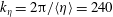 $k_{\unicode[STIX]{x1D702}}=2\unicode[STIX]{x03C0}/\langle \unicode[STIX]{x1D702}\rangle =240$
.
$k_{\unicode[STIX]{x1D702}}=2\unicode[STIX]{x03C0}/\langle \unicode[STIX]{x1D702}\rangle =240$
.
We observe in figure 2 that both
 $K(t)$
and
$K(t)$
and
 $\unicode[STIX]{x1D716}(t)$
oscillate significantly. Note that these significant fluctuations are contributed by all Fourier modes with larger wavenumbers than
$\unicode[STIX]{x1D716}(t)$
oscillate significantly. Note that these significant fluctuations are contributed by all Fourier modes with larger wavenumbers than
 $k_{F}=\sqrt{11}$
because of the fixing feature of the energy input mechanism (see (2.4)). We also find that
$k_{F}=\sqrt{11}$
because of the fixing feature of the energy input mechanism (see (2.4)). We also find that
 $K(t)$
has five peaks and peaks of
$K(t)$
has five peaks and peaks of
 $\unicode[STIX]{x1D716}(t)$
come after those of
$\unicode[STIX]{x1D716}(t)$
come after those of
 $K(t)$
. This time lag is due to energy transfer events from larger to smaller scales (van Veen et al.
Reference van Veen, Kida and Kawahara2006). Since the temporal standard deviation
$K(t)$
. This time lag is due to energy transfer events from larger to smaller scales (van Veen et al.
Reference van Veen, Kida and Kawahara2006). Since the temporal standard deviation
 $\unicode[STIX]{x1D70E}_{\unicode[STIX]{x1D716}}$
of
$\unicode[STIX]{x1D70E}_{\unicode[STIX]{x1D716}}$
of
 $\unicode[STIX]{x1D716}$
of the period-5 motion is comparable to that of turbulent motion, where
$\unicode[STIX]{x1D716}$
of the period-5 motion is comparable to that of turbulent motion, where
 $\unicode[STIX]{x1D70E}_{\unicode[STIX]{x1D716}}/[\langle u^{\prime }\rangle ^{3}/\langle L\rangle ]$
is 0.0253 for the former and 0.0480 for the latter, it is reasonable to investigate and discuss an oscillation mechanism by means of the period-5 motion.
$\unicode[STIX]{x1D70E}_{\unicode[STIX]{x1D716}}/[\langle u^{\prime }\rangle ^{3}/\langle L\rangle ]$
is 0.0253 for the former and 0.0480 for the latter, it is reasonable to investigate and discuss an oscillation mechanism by means of the period-5 motion.
Figure 3 gives a comparison of energy dissipation rate between high-symmetric turbulence and the time-periodic solutions. Clearly, the time-periodic solutions shown in the figure reproduce the time-mean energy dissipation rate of turbulence. A comparison of the time-averaged one-dimensional longitudinal energy spectra
 $\langle E_{||}\rangle (k)$
of turbulence and periodic motion with a resolution of
$\langle E_{||}\rangle (k)$
of turbulence and periodic motion with a resolution of
 $512^{3}$
is shown in figure 4, where
$512^{3}$
is shown in figure 4, where
 $E_{||}(k_{1},t)=(1/2)\sum _{k_{2},k_{3}}|\widetilde{u}_{1}(k_{1},k_{2},k_{3},t)|^{2}$
. The flow is well-resolved and the energy spectra are close to each other.
$E_{||}(k_{1},t)=(1/2)\sum _{k_{2},k_{3}}|\widetilde{u}_{1}(k_{1},k_{2},k_{3},t)|^{2}$
. The flow is well-resolved and the energy spectra are close to each other.
Apart from reducing the number of Fourier modes in the simulations, the imposed symmetries have the effect of fixing in space the larger-scale vortex, the central axis of which coincides with the diagonal of a fundamental box. As for the fundamental box whose domain is
 $0\leqslant x_{1},x_{2},x_{3}\leqslant \unicode[STIX]{x03C0}/2$
, the central axis coincides with the diagonal connecting the origin O to the point A
$0\leqslant x_{1},x_{2},x_{3}\leqslant \unicode[STIX]{x03C0}/2$
, the central axis coincides with the diagonal connecting the origin O to the point A
 $(\unicode[STIX]{x03C0}/2,\unicode[STIX]{x03C0}/2,\unicode[STIX]{x03C0}/2)$
. Besides that, the complexity of the time evolution of the flow field in a fundamental box is further reduced because of the
$(\unicode[STIX]{x03C0}/2,\unicode[STIX]{x03C0}/2,\unicode[STIX]{x03C0}/2)$
. Besides that, the complexity of the time evolution of the flow field in a fundamental box is further reduced because of the
 $2\unicode[STIX]{x03C0}/3$
rotational symmetry around the central axis.
$2\unicode[STIX]{x03C0}/3$
rotational symmetry around the central axis.
Finally, we discuss briefly the information on the structure of the unstable eigenvectors or the stability properties of the steady solution at
 $\unicode[STIX]{x1D708}=0.0035$
. We obtained the nonlinear equilibrium solution numerically by tracking a stable equilibrium solution for a large viscosity in
$\unicode[STIX]{x1D708}=0.0035$
. We obtained the nonlinear equilibrium solution numerically by tracking a stable equilibrium solution for a large viscosity in
 $\unicode[STIX]{x1D708}$
down to
$\unicode[STIX]{x1D708}$
down to
 $\unicode[STIX]{x1D708}=0.0035$
by using the arc-length continuation method and computed its leading eigenvector. The most unstable eigenvector contains most energy (by a factor greater than 10) in the forcing wavenumber shell
$\unicode[STIX]{x1D708}=0.0035$
by using the arc-length continuation method and computed its leading eigenvector. The most unstable eigenvector contains most energy (by a factor greater than 10) in the forcing wavenumber shell
 $|\boldsymbol{k}|=k_{F}$
. The solution has 18 unstable eigenvalues in total and seems unlikely to have much influence on the dynamics. Therefore, the steady solution does not have a significant impact on our proposed mechanism, which will appear in § 5.2.
$|\boldsymbol{k}|=k_{F}$
. The solution has 18 unstable eigenvalues in total and seems unlikely to have much influence on the dynamics. Therefore, the steady solution does not have a significant impact on our proposed mechanism, which will appear in § 5.2.

Figure 5. Cylindrical coordinate system
 $(r,\unicode[STIX]{x1D703},z)$
in the fundamental box
$(r,\unicode[STIX]{x1D703},z)$
in the fundamental box
 $0\leqslant x_{1},x_{2},x_{3}\leqslant \unicode[STIX]{x03C0}/2$
and the corresponding three unit vectors
$0\leqslant x_{1},x_{2},x_{3}\leqslant \unicode[STIX]{x03C0}/2$
and the corresponding three unit vectors
 $\boldsymbol{e}_{r}$
,
$\boldsymbol{e}_{r}$
,
 $\boldsymbol{e}_{\unicode[STIX]{x1D703}}$
and
$\boldsymbol{e}_{\unicode[STIX]{x1D703}}$
and
 $\boldsymbol{e}_{z}$
.
$\boldsymbol{e}_{z}$
.
3 Vortical structures in high-symmetric turbulence
In this section, we shall examine the vortical structures, i.e. the larger-scale vortices and smaller-scale vortices in high-symmetric turbulence at moderate Reynolds numbers. These vortices play an important role in the vortex interaction mechanism.
3.1 The larger-scale vortices
As previously seen in figure 1, the large-scale swirling flow around the diagonal of a fundamental box is sustained by fixing the amplitude of a number of Fourier coefficients in time (see (2.4)). Taking into account the flow characteristics, we decompose the velocity vector
 $\boldsymbol{u}$
and the vorticity vector
$\boldsymbol{u}$
and the vorticity vector
 $\unicode[STIX]{x1D74E}$
into three mutually perpendicular components in a cylindrical coordinate system
$\unicode[STIX]{x1D74E}$
into three mutually perpendicular components in a cylindrical coordinate system
 $(r,\unicode[STIX]{x1D703},z)$
whose longitudinal axis is defined by the diagonal line of a fundamental box (see figure 5). In the cylindrical coordinate system, velocity vector
$(r,\unicode[STIX]{x1D703},z)$
whose longitudinal axis is defined by the diagonal line of a fundamental box (see figure 5). In the cylindrical coordinate system, velocity vector
 $\boldsymbol{u}$
is expressed as
$\boldsymbol{u}$
is expressed as
 $\boldsymbol{u}=(u_{r},u_{\unicode[STIX]{x1D703}},u_{z})$
, where
$\boldsymbol{u}=(u_{r},u_{\unicode[STIX]{x1D703}},u_{z})$
, where
 $u_{r}$
is the radial velocity,
$u_{r}$
is the radial velocity,
 $u_{\unicode[STIX]{x1D703}}$
the circumferential velocity,
$u_{\unicode[STIX]{x1D703}}$
the circumferential velocity,
 $u_{z}$
the axial velocity. They are obtained by solving the following system of linear equations,
$u_{z}$
the axial velocity. They are obtained by solving the following system of linear equations,
 $$\begin{eqnarray}\displaystyle \left(\begin{array}{@{}c@{}}u_{r}\\ u_{\unicode[STIX]{x1D703}}\\ u_{z}\end{array}\right)=\left(\begin{array}{@{}ccc@{}}\boldsymbol{e}_{r} & \boldsymbol{e}_{\unicode[STIX]{x1D703}} & \boldsymbol{e}_{z}\end{array}\right)^{-1}\left(\begin{array}{@{}c@{}}u_{1}\\ u_{2}\\ u_{3}\end{array}\right), & & \displaystyle\end{eqnarray}$$
where the
 $3\times 3$
matrix, which is dependent upon
$3\times 3$
matrix, which is dependent upon
 $\boldsymbol{x}$
, is composed of the three unit vectors:
$\boldsymbol{x}$
, is composed of the three unit vectors:
 $\boldsymbol{e}_{r}=\boldsymbol{r}/|\boldsymbol{r}|=(\boldsymbol{x}-\boldsymbol{z})/|\boldsymbol{x}-\boldsymbol{z}|$
,
$\boldsymbol{e}_{r}=\boldsymbol{r}/|\boldsymbol{r}|=(\boldsymbol{x}-\boldsymbol{z})/|\boldsymbol{x}-\boldsymbol{z}|$
,
 $\boldsymbol{e}_{\unicode[STIX]{x1D703}}=(\boldsymbol{z}\times \boldsymbol{r})/|\boldsymbol{z}\times \boldsymbol{r}|$
and
$\boldsymbol{e}_{\unicode[STIX]{x1D703}}=(\boldsymbol{z}\times \boldsymbol{r})/|\boldsymbol{z}\times \boldsymbol{r}|$
and
 $\boldsymbol{e}_{z}=\boldsymbol{z}/|\boldsymbol{z}|=1/\sqrt{3}(1,1,1)$
. Vorticity vector
$\boldsymbol{e}_{z}=\boldsymbol{z}/|\boldsymbol{z}|=1/\sqrt{3}(1,1,1)$
. Vorticity vector
 $\unicode[STIX]{x1D74E}$
is similarly expressed as
$\unicode[STIX]{x1D74E}$
is similarly expressed as
 $\unicode[STIX]{x1D74E}=(\unicode[STIX]{x1D714}_{r},\unicode[STIX]{x1D714}_{\unicode[STIX]{x1D703}},\unicode[STIX]{x1D714}_{z})$
, where
$\unicode[STIX]{x1D74E}=(\unicode[STIX]{x1D714}_{r},\unicode[STIX]{x1D714}_{\unicode[STIX]{x1D703}},\unicode[STIX]{x1D714}_{z})$
, where
 $\unicode[STIX]{x1D714}_{r}$
is the radial vorticity,
$\unicode[STIX]{x1D714}_{r}$
is the radial vorticity,
 $\unicode[STIX]{x1D714}_{\unicode[STIX]{x1D703}}$
the circumferential vorticity and
$\unicode[STIX]{x1D714}_{\unicode[STIX]{x1D703}}$
the circumferential vorticity and
 $\unicode[STIX]{x1D714}_{z}$
the axial vorticity. Figure 6 shows the time evolutions of
$\unicode[STIX]{x1D714}_{z}$
the axial vorticity. Figure 6 shows the time evolutions of
 $\langle u_{r}^{2}\rangle _{f}$
,
$\langle u_{r}^{2}\rangle _{f}$
,
 $\langle u_{\unicode[STIX]{x1D703}}^{2}\rangle _{f}$
and
$\langle u_{\unicode[STIX]{x1D703}}^{2}\rangle _{f}$
and
 $\langle u_{z}^{2}\rangle _{f}$
as well as
$\langle u_{z}^{2}\rangle _{f}$
as well as
 $\langle \unicode[STIX]{x1D714}_{r}^{2}\rangle _{f}$
,
$\langle \unicode[STIX]{x1D714}_{r}^{2}\rangle _{f}$
,
 $\langle \unicode[STIX]{x1D714}_{\unicode[STIX]{x1D703}}^{2}\rangle _{f}$
and
$\langle \unicode[STIX]{x1D714}_{\unicode[STIX]{x1D703}}^{2}\rangle _{f}$
and
 $\langle \unicode[STIX]{x1D714}_{z}^{2}\rangle _{f}$
for the period-5 motion, where
$\langle \unicode[STIX]{x1D714}_{z}^{2}\rangle _{f}$
for the period-5 motion, where
 $\langle \cdot \rangle _{f}$
indicates the spatially averaged value over the fundamental box (
$\langle \cdot \rangle _{f}$
indicates the spatially averaged value over the fundamental box (
 $0\leqslant x_{1},x_{2},x_{3}\leqslant \unicode[STIX]{x03C0}/2$
). Over the whole time period, the temporal mean of
$0\leqslant x_{1},x_{2},x_{3}\leqslant \unicode[STIX]{x03C0}/2$
). Over the whole time period, the temporal mean of
 $\langle u_{\unicode[STIX]{x1D703}}^{2}\rangle _{f}$
is much larger than those of
$\langle u_{\unicode[STIX]{x1D703}}^{2}\rangle _{f}$
is much larger than those of
 $\langle u_{r}^{2}\rangle _{f}$
and
$\langle u_{r}^{2}\rangle _{f}$
and
 $\langle u_{z}^{2}\rangle _{f}$
, and that of
$\langle u_{z}^{2}\rangle _{f}$
, and that of
 $\langle \unicode[STIX]{x1D714}_{z}^{2}\rangle _{f}$
is much larger than those of
$\langle \unicode[STIX]{x1D714}_{z}^{2}\rangle _{f}$
is much larger than those of
 $\langle \unicode[STIX]{x1D714}_{r}^{2}\rangle _{f}$
and
$\langle \unicode[STIX]{x1D714}_{r}^{2}\rangle _{f}$
and
 $\langle \unicode[STIX]{x1D714}_{\unicode[STIX]{x1D703}}^{2}\rangle _{f}$
. It is therefore considered that, in a fundamental box, the swirling flow around the diagonal is dominant and the corresponding columnar vortex is the dominant flow structure. Hereinafter, we shall refer to the columnar vortex as the larger-scale vortex. It is statistically sustained by the external forcing preserving a high-symmetric flow field (Kida Reference Kida1985). Figure 6(a) also shows that
$\langle \unicode[STIX]{x1D714}_{\unicode[STIX]{x1D703}}^{2}\rangle _{f}$
. It is therefore considered that, in a fundamental box, the swirling flow around the diagonal is dominant and the corresponding columnar vortex is the dominant flow structure. Hereinafter, we shall refer to the columnar vortex as the larger-scale vortex. It is statistically sustained by the external forcing preserving a high-symmetric flow field (Kida Reference Kida1985). Figure 6(a) also shows that
 $\langle u_{\unicode[STIX]{x1D703}}^{2}\rangle _{f}$
fluctuates around its temporal mean with large amplitude and shows five peaks. The global intensity of the large-scale swirling flow over the fundamental box becomes active and quiescent alternately corresponding to the time variation of
$\langle u_{\unicode[STIX]{x1D703}}^{2}\rangle _{f}$
fluctuates around its temporal mean with large amplitude and shows five peaks. The global intensity of the large-scale swirling flow over the fundamental box becomes active and quiescent alternately corresponding to the time variation of
 $\langle u_{\unicode[STIX]{x1D703}}^{2}\rangle _{f}$
. Incidentally, the last two large-amplitude oscillations of
$\langle u_{\unicode[STIX]{x1D703}}^{2}\rangle _{f}$
. Incidentally, the last two large-amplitude oscillations of
 $\langle \unicode[STIX]{x1D714}_{\unicode[STIX]{x1D703}}^{2}\rangle$
correspond to generation and circumferential vortex stretching of strong smaller-scale vortices, which will be presented in the next subsection (§ 3.2).
$\langle \unicode[STIX]{x1D714}_{\unicode[STIX]{x1D703}}^{2}\rangle$
correspond to generation and circumferential vortex stretching of strong smaller-scale vortices, which will be presented in the next subsection (§ 3.2).

Figure 6. Time evolutions of the spatially averaged quantities over the fundamental box (
 $0\leqslant x_{1},x_{2},x_{3}\leqslant \unicode[STIX]{x03C0}/2$
). (a) Blue dash-dotted,
$0\leqslant x_{1},x_{2},x_{3}\leqslant \unicode[STIX]{x03C0}/2$
). (a) Blue dash-dotted,
 $\langle u_{r}^{2}\rangle _{f}/[2\langle K\rangle ]$
; green solid,
$\langle u_{r}^{2}\rangle _{f}/[2\langle K\rangle ]$
; green solid,
 $\langle u_{\unicode[STIX]{x1D703}}^{2}\rangle _{f}/[2\langle K\rangle ]$
; red dashed,
$\langle u_{\unicode[STIX]{x1D703}}^{2}\rangle _{f}/[2\langle K\rangle ]$
; red dashed,
 $\langle u_{z}^{2}\rangle _{f}/[2\langle K\rangle ]$
. (b) Blue dash-dotted,
$\langle u_{z}^{2}\rangle _{f}/[2\langle K\rangle ]$
. (b) Blue dash-dotted,
 $\langle \unicode[STIX]{x1D714}_{r}^{2}\rangle _{f}/[2\langle {\mathcal{Q}}\rangle ]$
; green solid,
$\langle \unicode[STIX]{x1D714}_{r}^{2}\rangle _{f}/[2\langle {\mathcal{Q}}\rangle ]$
; green solid,
 $\langle \unicode[STIX]{x1D714}_{\unicode[STIX]{x1D703}}^{2}\rangle _{f}/[2\langle {\mathcal{Q}}\rangle ]$
; red dashed,
$\langle \unicode[STIX]{x1D714}_{\unicode[STIX]{x1D703}}^{2}\rangle _{f}/[2\langle {\mathcal{Q}}\rangle ]$
; red dashed,
 $\langle \unicode[STIX]{x1D714}_{z}^{2}\rangle _{f}/[2\langle {\mathcal{Q}}\rangle ]$
.
$\langle \unicode[STIX]{x1D714}_{z}^{2}\rangle _{f}/[2\langle {\mathcal{Q}}\rangle ]$
.
The period-5 motion includes active and quiescent periods of time. Since we will later discuss the closed regenerative cycle of the large-amplitude axial waves, which is reminiscent of the regeneration cycle of near-wall turbulence structures (Hamilton et al.
Reference Hamilton, Kim and Waleffe1995), it is convenient to have a well-defined period of time. In this paper, by focusing on the time evolution of the global intensity of the large-scale swirling flow over the fundamental box, we define a single cycle as the time period from one time when
 $\langle u_{\unicode[STIX]{x1D703}}^{2}\rangle _{f}$
attains a local maximum to the time when it attains the next local one. Figure 7 shows the time period (
$\langle u_{\unicode[STIX]{x1D703}}^{2}\rangle _{f}$
attains a local maximum to the time when it attains the next local one. Figure 7 shows the time period (
 $6.27\leqslant t/T\leqslant 9.18$
) including one of the five cycles during which the most intense energy dissipation event takes place. During this time period,
$6.27\leqslant t/T\leqslant 9.18$
) including one of the five cycles during which the most intense energy dissipation event takes place. During this time period,
 $\langle u_{\unicode[STIX]{x1D703}}^{2}\rangle _{f}$
attains its local maxima at
$\langle u_{\unicode[STIX]{x1D703}}^{2}\rangle _{f}$
attains its local maxima at
 $t=t_{1}$
and
$t=t_{1}$
and
 $t_{7}$
, and its local minimum at
$t_{7}$
, and its local minimum at
 $t=t_{4}$
;
$t=t_{4}$
;
 $\unicode[STIX]{x1D716}$
attains its local maximum at
$\unicode[STIX]{x1D716}$
attains its local maximum at
 $t=t_{2}$
and its local minimum at
$t=t_{2}$
and its local minimum at
 $t=t_{5}$
. This time period will be used when investigating the oscillatory evolution in detail in § 5. Here, it is important to emphasise that, although we select it for investigation, our proposed mechanism, a vortex interaction mechanism, plays an important role in generating global oscillations whether or not the period includes the most intense energy dissipation event. Indeed, in § 6 we will find its significance even in decaying high-symmetric turbulence whose turbulence intensity is significantly decreasing with time.
$t=t_{5}$
. This time period will be used when investigating the oscillatory evolution in detail in § 5. Here, it is important to emphasise that, although we select it for investigation, our proposed mechanism, a vortex interaction mechanism, plays an important role in generating global oscillations whether or not the period includes the most intense energy dissipation event. Indeed, in § 6 we will find its significance even in decaying high-symmetric turbulence whose turbulence intensity is significantly decreasing with time.

Figure 7. Time evolutions of
 $\langle u_{\unicode[STIX]{x1D703}}^{2}\rangle _{f}$
(green solid line) and the total energy dissipation rate
$\langle u_{\unicode[STIX]{x1D703}}^{2}\rangle _{f}$
(green solid line) and the total energy dissipation rate
 $\unicode[STIX]{x1D716}$
(blue dashed line) (
$\unicode[STIX]{x1D716}$
(blue dashed line) (
 $6.27\leqslant t/T\leqslant 9.18$
). The seven dashed straight lines from left to right indicate times
$6.27\leqslant t/T\leqslant 9.18$
). The seven dashed straight lines from left to right indicate times
 $t_{1}-t_{7}$
:
$t_{1}-t_{7}$
:
 $t_{1}=6.74T$
,
$t_{1}=6.74T$
,
 $t_{2}=7.04T$
,
$t_{2}=7.04T$
,
 $t_{3}=7.40T$
,
$t_{3}=7.40T$
,
 $t_{4}=7.66T$
,
$t_{4}=7.66T$
,
 $t_{5}=8.09T$
,
$t_{5}=8.09T$
,
 $t_{6}=8.38T$
and
$t_{6}=8.38T$
and
 $t_{7}=8.70T$
.
$t_{7}=8.70T$
.
 $\langle u_{\unicode[STIX]{x1D703}}^{2}\rangle _{f}$
attains its local maxima at
$\langle u_{\unicode[STIX]{x1D703}}^{2}\rangle _{f}$
attains its local maxima at
 $t=t_{1}$
and
$t=t_{1}$
and
 $t_{7}$
and its local minimum at
$t_{7}$
and its local minimum at
 $t=t_{4}$
.
$t=t_{4}$
.
 $\unicode[STIX]{x1D716}$
attains its local maximum at
$\unicode[STIX]{x1D716}$
attains its local maximum at
 $t=t_{2}$
and its local minimum at
$t=t_{2}$
and its local minimum at
 $t=t_{5}$
.
$t=t_{5}$
.
3.2 The smaller-scale vortices
3.2.1 Classification of smaller-scale vortices
Here, we shall introduce the smaller-scale vortices, the dynamics of which is spatio-temporally simplified because of the symmetry constraint. We shall consider smaller-scale vortices in the fundamental box (
 $0\leqslant x_{1},x_{2},x_{3}\leqslant \unicode[STIX]{x03C0}/2$
). At this moderate Reynolds number (
$0\leqslant x_{1},x_{2},x_{3}\leqslant \unicode[STIX]{x03C0}/2$
). At this moderate Reynolds number (
 $\langle R_{\unicode[STIX]{x1D706}}\rangle =69.6$
), we can classify all the smaller-scale vortices into two types, both of which are generated and stretched in the strong straining fields appearing between the larger-scale vortices. Vortices of one type are created in the strong straining fields near the origin O while vortices of the other type are created in those near the point
$\langle R_{\unicode[STIX]{x1D706}}\rangle =69.6$
), we can classify all the smaller-scale vortices into two types, both of which are generated and stretched in the strong straining fields appearing between the larger-scale vortices. Vortices of one type are created in the strong straining fields near the origin O while vortices of the other type are created in those near the point
 $\text{A}(\unicode[STIX]{x03C0}/2,\unicode[STIX]{x03C0}/2,\unicode[STIX]{x03C0}/2)$
. Recall that the generation mechanism of smaller-scale vortices in strong straining regions between the larger-scale vortices was previously reported by means of DNS of homogeneous isotropic turbulence at higher Reynolds numbers (Goto Reference Goto2008, Reference Goto2012; Leung, Swaminathan & Davidson Reference Leung, Swaminathan and Davidson2012; Goto, Saito & Kawahara Reference Goto, Saito and Kawahara2017) and is not specific to high-symmetric turbulence. Once they are created in such a way, the former vortices start to move towards the origin O and the latter towards the point A. Therefore, we hereinafter refer to the former group of vortices as SV-O and the latter as SV-A. Note that both the origin O and the point A are stagnation points of the velocity vector field. In order to grasp the spatial arrangement of smaller-scale vortices, we plot in figure 8 an instantaneous flow field of the period-5 motion in the 64 fundamental boxes (
$\text{A}(\unicode[STIX]{x03C0}/2,\unicode[STIX]{x03C0}/2,\unicode[STIX]{x03C0}/2)$
. Recall that the generation mechanism of smaller-scale vortices in strong straining regions between the larger-scale vortices was previously reported by means of DNS of homogeneous isotropic turbulence at higher Reynolds numbers (Goto Reference Goto2008, Reference Goto2012; Leung, Swaminathan & Davidson Reference Leung, Swaminathan and Davidson2012; Goto, Saito & Kawahara Reference Goto, Saito and Kawahara2017) and is not specific to high-symmetric turbulence. Once they are created in such a way, the former vortices start to move towards the origin O and the latter towards the point A. Therefore, we hereinafter refer to the former group of vortices as SV-O and the latter as SV-A. Note that both the origin O and the point A are stagnation points of the velocity vector field. In order to grasp the spatial arrangement of smaller-scale vortices, we plot in figure 8 an instantaneous flow field of the period-5 motion in the 64 fundamental boxes (
 $-\unicode[STIX]{x03C0}\leqslant x_{1},x_{2},x_{3}\leqslant \unicode[STIX]{x03C0}$
). The cubic domain drawn by thick black lines is
$-\unicode[STIX]{x03C0}\leqslant x_{1},x_{2},x_{3}\leqslant \unicode[STIX]{x03C0}$
). The cubic domain drawn by thick black lines is
 $-\unicode[STIX]{x03C0}/4\leqslant x_{1},x_{2},x_{3}\leqslant \unicode[STIX]{x03C0}/4$
, whose centre is the origin O, towards which the SV-O vortices converge. The cuboid domain drawn by thick red lines is the two fundamental boxes (
$-\unicode[STIX]{x03C0}/4\leqslant x_{1},x_{2},x_{3}\leqslant \unicode[STIX]{x03C0}/4$
, whose centre is the origin O, towards which the SV-O vortices converge. The cuboid domain drawn by thick red lines is the two fundamental boxes (
 $0\leqslant x_{1}\leqslant \unicode[STIX]{x03C0}$
and
$0\leqslant x_{1}\leqslant \unicode[STIX]{x03C0}$
and
 $0\leqslant x_{2},x_{3}\leqslant \unicode[STIX]{x03C0}/2$
). In this domain, we observe not only the SV-O but also SV-A vortices which converge towards the point A.
$0\leqslant x_{2},x_{3}\leqslant \unicode[STIX]{x03C0}/2$
). In this domain, we observe not only the SV-O but also SV-A vortices which converge towards the point A.

Figure 8. Snapshot of the flow field of the period-5 motion taken at
 $t/T=4.47$
. The largest cubic domain drawn by thin black lines (64 fundamental boxes) is
$t/T=4.47$
. The largest cubic domain drawn by thin black lines (64 fundamental boxes) is
 $-\unicode[STIX]{x03C0}\leqslant x_{1},x_{2},x_{3}\leqslant \unicode[STIX]{x03C0}$
. The cubic subdomain drawn by thick black lines is
$-\unicode[STIX]{x03C0}\leqslant x_{1},x_{2},x_{3}\leqslant \unicode[STIX]{x03C0}$
. The cubic subdomain drawn by thick black lines is
 $-\unicode[STIX]{x03C0}/4\leqslant x_{1},x_{2},x_{3}\leqslant \unicode[STIX]{x03C0}/4$
, whose centre is the origin O, which will appear in figure 9. The cuboid subdomain drawn by thick red lines is
$-\unicode[STIX]{x03C0}/4\leqslant x_{1},x_{2},x_{3}\leqslant \unicode[STIX]{x03C0}/4$
, whose centre is the origin O, which will appear in figure 9. The cuboid subdomain drawn by thick red lines is
 $0\leqslant x_{1}\leqslant \unicode[STIX]{x03C0}$
and
$0\leqslant x_{1}\leqslant \unicode[STIX]{x03C0}$
and
 $0\leqslant x_{2},x_{3}\leqslant \unicode[STIX]{x03C0}/2$
, which will be shown in figure 10. The smaller-scale vortices are visualised by grey-coloured isosurfaces of
$0\leqslant x_{2},x_{3}\leqslant \unicode[STIX]{x03C0}/2$
, which will be shown in figure 10. The smaller-scale vortices are visualised by grey-coloured isosurfaces of
 $|\unicode[STIX]{x1D74E}|^{2}/\langle \unicode[STIX]{x1D714}^{\prime }\rangle ^{2}=12$
, but they are coloured in green inside the subdomains. The blue-coloured plane including three points O, A
$|\unicode[STIX]{x1D74E}|^{2}/\langle \unicode[STIX]{x1D714}^{\prime }\rangle ^{2}=12$
, but they are coloured in green inside the subdomains. The blue-coloured plane including three points O, A
 $(\unicode[STIX]{x03C0}/2,\unicode[STIX]{x03C0}/2,\unicode[STIX]{x03C0}/2)$
and
$(\unicode[STIX]{x03C0}/2,\unicode[STIX]{x03C0}/2,\unicode[STIX]{x03C0}/2)$
and
 $(0,\unicode[STIX]{x03C0}/2,0)$
will be used in figures 17 and 18.
$(0,\unicode[STIX]{x03C0}/2,0)$
will be used in figures 17 and 18.

Figure 9. Snapshots of the flow fields in the cubic domain
 $-\unicode[STIX]{x03C0}/4\leqslant x_{1},x_{2},x_{3}\leqslant \unicode[STIX]{x03C0}/4$
whose centroid is the origin O. They are taken at (a)
$-\unicode[STIX]{x03C0}/4\leqslant x_{1},x_{2},x_{3}\leqslant \unicode[STIX]{x03C0}/4$
whose centroid is the origin O. They are taken at (a)
 $t=8.29T$
, (b)
$t=8.29T$
, (b)
 $8.78T$
, (c)
$8.78T$
, (c)
 $9.14T$
, (d)
$9.14T$
, (d)
 $9.32T$
, (e)
$9.32T$
, (e)
 $9.45T$
, (f)
$9.45T$
, (f)
 $9.68T$
. The grey and green isosurfaces indicate pressure
$9.68T$
. The grey and green isosurfaces indicate pressure
 $p/[\unicode[STIX]{x1D70C}\langle u^{\prime }\rangle ^{2}]=-2$
and
$p/[\unicode[STIX]{x1D70C}\langle u^{\prime }\rangle ^{2}]=-2$
and
 $|\unicode[STIX]{x1D74E}|^{2}/\langle \unicode[STIX]{x1D714}^{\prime }\rangle ^{2}=18$
, respectively. The streamlines of the instantaneous velocity fields are shown, where the red ones are in the domain
$|\unicode[STIX]{x1D74E}|^{2}/\langle \unicode[STIX]{x1D714}^{\prime }\rangle ^{2}=18$
, respectively. The streamlines of the instantaneous velocity fields are shown, where the red ones are in the domain
 $0\leqslant x_{1},x_{2},x_{3}\leqslant \unicode[STIX]{x03C0}/4$
and the blue ones are in the domain
$0\leqslant x_{1},x_{2},x_{3}\leqslant \unicode[STIX]{x03C0}/4$
and the blue ones are in the domain
 $0\leqslant x_{1},x_{3}\leqslant \unicode[STIX]{x03C0}/4$
and
$0\leqslant x_{1},x_{3}\leqslant \unicode[STIX]{x03C0}/4$
and
 $-\unicode[STIX]{x03C0}/4\leqslant x_{2}\leqslant 0$
. The mirror symmetries with respect to the three planes
$-\unicode[STIX]{x03C0}/4\leqslant x_{2}\leqslant 0$
. The mirror symmetries with respect to the three planes
 $x_{1}=0$
,
$x_{1}=0$
,
 $x_{2}=0$
and
$x_{2}=0$
and
 $x_{3}=0$
are observed. (a) The arrows show the rotation directions of the large-scale swirling flows. (b) The arrows indicate a counter-rotating vortex pair (a dipole).
$x_{3}=0$
are observed. (a) The arrows show the rotation directions of the large-scale swirling flows. (b) The arrows indicate a counter-rotating vortex pair (a dipole).

Figure 10. Snapshots of the flow fields in the two neighbouring fundamental boxes (
 $0\leqslant x_{1}\leqslant \unicode[STIX]{x03C0}$
and
$0\leqslant x_{1}\leqslant \unicode[STIX]{x03C0}$
and
 $0\leqslant x_{2},x_{3}\leqslant \unicode[STIX]{x03C0}/2$
). They are taken at (a)
$0\leqslant x_{2},x_{3}\leqslant \unicode[STIX]{x03C0}/2$
). They are taken at (a)
 $t=8.06T$
, (b)
$t=8.06T$
, (b)
 $8.19T$
, (c)
$8.19T$
, (c)
 $8.37T$
, (d)
$8.37T$
, (d)
 $8.51T$
, (e)
$8.51T$
, (e)
 $8.82T$
and (f)
$8.82T$
and (f)
 $9.40T$
. The light-grey, dark-grey and green isosurfaces indicate
$9.40T$
. The light-grey, dark-grey and green isosurfaces indicate
 $p/[\unicode[STIX]{x1D70C}\langle u^{\prime }\rangle ^{2}]=-2$
,
$p/[\unicode[STIX]{x1D70C}\langle u^{\prime }\rangle ^{2}]=-2$
,
 $\unicode[STIX]{x1D61A}_{ij}\unicode[STIX]{x1D61A}_{ij}/\langle \unicode[STIX]{x1D714}^{\prime }\rangle ^{2}=12$
and
$\unicode[STIX]{x1D61A}_{ij}\unicode[STIX]{x1D61A}_{ij}/\langle \unicode[STIX]{x1D714}^{\prime }\rangle ^{2}=12$
and
 $|\unicode[STIX]{x1D74E}|^{2}/\langle \unicode[STIX]{x1D714}^{\prime }\rangle ^{2}=18$
, respectively. The red streamlines of the instantaneous velocity fields are shown. (a) The arrows show the rotation direction of the large-scale swirling flows. (c) The elliptic area denoted by B indicates the region where strong straining fields are generated. (d) The arrows indicate a counter-rotating vortex pair (a dipole). (e) The double arrow shows the directions of stretching by the larger-scale vortices. The SV-A vortices are observed in the shape of the letter S being wrapped around the larger-scale vortices.
$|\unicode[STIX]{x1D74E}|^{2}/\langle \unicode[STIX]{x1D714}^{\prime }\rangle ^{2}=18$
, respectively. The red streamlines of the instantaneous velocity fields are shown. (a) The arrows show the rotation direction of the large-scale swirling flows. (c) The elliptic area denoted by B indicates the region where strong straining fields are generated. (d) The arrows indicate a counter-rotating vortex pair (a dipole). (e) The double arrow shows the directions of stretching by the larger-scale vortices. The SV-A vortices are observed in the shape of the letter S being wrapped around the larger-scale vortices.
These vortices are similar to those in decaying high-symmetric turbulence which were previously found and investigated by Boratav & Pelz (Reference Boratav and Pelz1994, Reference Boratav and Pelz1995). They performed DNS of decaying turbulence which starts with the initial velocity field (2.5), and observed the smaller-scale vortices moving towards the stagnation points. In the following, we will consider time evolutions of the SV-O and SV-A vortices in high-symmetric flow with the external forcing (2.4).
3.2.2 Time evolutions and creation mechanisms of the SV-O and SV-A vortices
Firstly, we shall consider the time evolution and creation mechanism of the SV-O vortices. Figure 9 shows the time evolution of the SV-O vortices visualised by isosurfaces of enstrophy and the larger-scale vortices visualised by isosurfaces of low pressure. To provide the information of the three-dimensional velocity field, we also plot streamlines of the instantaneous velocity field. Since the velocity field has three mirror symmetries with respect to three planes
 $x_{1}=0$
,
$x_{1}=0$
,
 $x_{2}=0$
and
$x_{2}=0$
and
 $x_{3}=0$
, the origin O is a stagnation point of the velocity vector field. This point is surrounded by the eight large-scale swirling flows with different orientations. Because of the arrangement of the larger-scale swirling flows, strong straining fields tend to be generated near three planes
$x_{3}=0$
, the origin O is a stagnation point of the velocity vector field. This point is surrounded by the eight large-scale swirling flows with different orientations. Because of the arrangement of the larger-scale swirling flows, strong straining fields tend to be generated near three planes
 $x_{1}=0$
,
$x_{1}=0$
,
 $x_{2}=0$
and
$x_{2}=0$
and
 $x_{3}=0$
. The SV-O vortices are stretched and created in the straining fields generated by local high-speed rotational motions around the central axis of the larger-scale vortices (see figure 9
a); they appear in the form of counter-rotating vortex pairs (dipoles) (figure 9
b). It is confirmed that, once they are created, the SV-O vortices start to converge towards the origin O (figure 9
b–e). This convergence of the SV-O vortices has been explained in terms of the mutual induction between the 12 vortices (six dipoles) (Boratav & Pelz Reference Boratav and Pelz1995; Pelz Reference Pelz2001; Kimura Reference Kimura2010). In the late stage of their convergence, they dissipate and diminish strongly affected by viscosity; in the meantime, the new SV-O vortices are generated far from the origin O as seen in figure 9(f). This is the beginning of the next cycle.
$x_{3}=0$
. The SV-O vortices are stretched and created in the straining fields generated by local high-speed rotational motions around the central axis of the larger-scale vortices (see figure 9
a); they appear in the form of counter-rotating vortex pairs (dipoles) (figure 9
b). It is confirmed that, once they are created, the SV-O vortices start to converge towards the origin O (figure 9
b–e). This convergence of the SV-O vortices has been explained in terms of the mutual induction between the 12 vortices (six dipoles) (Boratav & Pelz Reference Boratav and Pelz1995; Pelz Reference Pelz2001; Kimura Reference Kimura2010). In the late stage of their convergence, they dissipate and diminish strongly affected by viscosity; in the meantime, the new SV-O vortices are generated far from the origin O as seen in figure 9(f). This is the beginning of the next cycle.
Secondly, we discuss the SV-A vortices. In a fundamental box, we can only observe parts of the SV-A vortices. In order to observe the whole picture of the individual SV-A vortices, it is necessary to consider neighbouring fundamental boxes. This is because these vortices cross a boundary plane between two fundamental boxes. As for the fundamental box whose spatial domain is
 $0\leqslant x_{1},x_{2},x_{3}\leqslant \unicode[STIX]{x03C0}/2$
, the SV-A vortices cross three planes:
$0\leqslant x_{1},x_{2},x_{3}\leqslant \unicode[STIX]{x03C0}/2$
, the SV-A vortices cross three planes:
 $x_{1}=\unicode[STIX]{x03C0}/2$
,
$x_{1}=\unicode[STIX]{x03C0}/2$
,
 $x_{2}=\unicode[STIX]{x03C0}/2$
and
$x_{2}=\unicode[STIX]{x03C0}/2$
and
 $x_{3}=\unicode[STIX]{x03C0}/2$
. In the following, therefore, we shall consider the flow field in the two neighbouring fundamental boxes whose domain is
$x_{3}=\unicode[STIX]{x03C0}/2$
. In the following, therefore, we shall consider the flow field in the two neighbouring fundamental boxes whose domain is
 $0\leqslant x_{1}\leqslant \unicode[STIX]{x03C0}$
and
$0\leqslant x_{1}\leqslant \unicode[STIX]{x03C0}$
and
 $0\leqslant x_{2},x_{3}\leqslant \unicode[STIX]{x03C0}/2$
, where the whole picture of the SV-A vortices crossing the plane
$0\leqslant x_{2},x_{3}\leqslant \unicode[STIX]{x03C0}/2$
, where the whole picture of the SV-A vortices crossing the plane
 $x_{1}=\unicode[STIX]{x03C0}/2$
is observed.
$x_{1}=\unicode[STIX]{x03C0}/2$
is observed.
Figure 10 shows the time evolution of the SV-A vortices. The two larger-scale vortices in the left and right fundamental boxes are visualised by the light-grey isosurfaces of low pressure surrounded by streamlines of the instantaneous velocity field, and the SV-A vortices are visualised by the green isosurfaces of enstrophy; the strong straining flow fields are visualised by the dark-grey isosurfaces of
 $\unicode[STIX]{x1D61A}_{ij}\unicode[STIX]{x1D61A}_{ij}$
, where
$\unicode[STIX]{x1D61A}_{ij}\unicode[STIX]{x1D61A}_{ij}$
, where
 $\unicode[STIX]{x1D61A}_{ij}=1/2(\unicode[STIX]{x2202}u_{i}/\unicode[STIX]{x2202}x_{j}+\unicode[STIX]{x2202}u_{j}/\unicode[STIX]{x2202}x_{i})$
is the strain-rate tensor. The boundary plane
$\unicode[STIX]{x1D61A}_{ij}=1/2(\unicode[STIX]{x2202}u_{i}/\unicode[STIX]{x2202}x_{j}+\unicode[STIX]{x2202}u_{j}/\unicode[STIX]{x2202}x_{i})$
is the strain-rate tensor. The boundary plane
 $x_{1}=\unicode[STIX]{x03C0}/2$
between the two adjacent fundamental boxes is located between the two identical large-scale swirling flows with different orientations. When local rotational motions near the point A start to get faster, strong straining fields are generated near the plane
$x_{1}=\unicode[STIX]{x03C0}/2$
between the two adjacent fundamental boxes is located between the two identical large-scale swirling flows with different orientations. When local rotational motions near the point A start to get faster, strong straining fields are generated near the plane
 $x_{1}=\unicode[STIX]{x03C0}/2$
(see the region B in figure 10
c). In the vicinity of the strong strain fields, the two SV-A vortices are created in the form of a counter-rotating vortex pair (a dipole) and converge towards the stagnation point A being rolled up by the larger-scale vortices (a counter-rotating vortex pair is denoted by the yellow arrows in figure 10
d). This convergence may be caused by the mutual induction of the SV-A vortices as in the case of the SV-O vortices. As a result of being wrapped around the larger-scale vortex, the isosurfaces of enstrophy are formed in the shape of the letter S (see figure 10
e). Eventually, the SV-A vortices dissipate because of viscosity. Although not shown in figure 10, a total of 24 SV-A vortices (12 dipoles) in the eight neighbouring fundamental boxes approach the stagnation point A.
$x_{1}=\unicode[STIX]{x03C0}/2$
(see the region B in figure 10
c). In the vicinity of the strong strain fields, the two SV-A vortices are created in the form of a counter-rotating vortex pair (a dipole) and converge towards the stagnation point A being rolled up by the larger-scale vortices (a counter-rotating vortex pair is denoted by the yellow arrows in figure 10
d). This convergence may be caused by the mutual induction of the SV-A vortices as in the case of the SV-O vortices. As a result of being wrapped around the larger-scale vortex, the isosurfaces of enstrophy are formed in the shape of the letter S (see figure 10
e). Eventually, the SV-A vortices dissipate because of viscosity. Although not shown in figure 10, a total of 24 SV-A vortices (12 dipoles) in the eight neighbouring fundamental boxes approach the stagnation point A.
Note that, although we have selected to demonstrate the six snapshots which are taken from one of the five cyclic events, qualitatively similar spatio-temporal evolutions of SV-O and SV-A vortices are also observed in the other events.
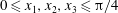
Figure 11. (a) Time evolution of energy spectrum of the period-5 motion. The horizontal and longitudinal axes represent the time and wavenumber, respectively. The contours are not shown in the wavenumber range beyond
 $k=70$
for clarity. (b) Temporal fluctuations of global quantities around their temporal mean normalised by their temporal standard deviation. The grey, green, red and blue lines correspond to
$k=70$
for clarity. (b) Temporal fluctuations of global quantities around their temporal mean normalised by their temporal standard deviation. The grey, green, red and blue lines correspond to
 $E(k=6,t)$
,
$E(k=6,t)$
,
 $\langle u_{\unicode[STIX]{x1D703}}^{2}\rangle _{f}(t)$
,
$\langle u_{\unicode[STIX]{x1D703}}^{2}\rangle _{f}(t)$
,
 $K(t)$
and
$K(t)$
and
 $\unicode[STIX]{x1D716}(t)$
, respectively. (a,b) The five dashed straight lines indicate the times when
$\unicode[STIX]{x1D716}(t)$
, respectively. (a,b) The five dashed straight lines indicate the times when
 $E(k=6,t)$
attains its local maximum. The times are
$E(k=6,t)$
attains its local maximum. The times are
 $t=0.0793T$
,
$t=0.0793T$
,
 $1.95T$
,
$1.95T$
,
 $4.02T$
,
$4.02T$
,
 $5.95T$
and
$5.95T$
and
 $7.75T$
from left to right.
$7.75T$
from left to right.
4 Cyclic energy transfer dynamics and the origin of fluctuations
In this section, we shall further investigate features of temporal oscillations of the period-5 motion and discuss their relation to the observed primary flow structures: the larger-scale and smaller-scale vortices.
4.1 Cyclic energy transfer dynamics
In figure 11(a), we show the time evolution of three-dimensional energy spectrum
 $E(k,t)$
of the period-5 motion, as was shown by van Veen et al. (Reference van Veen, Kida and Kawahara2006). This contour plot demonstrates that fluctuating energy is transferred from smaller to larger wavenumbers in the high-wavenumber dissipation range (i.e. forward energy transfer). Our new finding in this plot is the presence of large-amplitude temporal fluctuation in
$E(k,t)$
of the period-5 motion, as was shown by van Veen et al. (Reference van Veen, Kida and Kawahara2006). This contour plot demonstrates that fluctuating energy is transferred from smaller to larger wavenumbers in the high-wavenumber dissipation range (i.e. forward energy transfer). Our new finding in this plot is the presence of large-amplitude temporal fluctuation in
 $E(k=6,t)$
, which has five peaks at times
$E(k=6,t)$
, which has five peaks at times
 $t=0.0793T$
,
$t=0.0793T$
,
 $1.95T$
,
$1.95T$
,
 $4.02T$
,
$4.02T$
,
 $5.95T$
and
$5.95T$
and
 $7.75T$
. Here, the wavenumber
$7.75T$
. Here, the wavenumber
 $k=6$
is smaller than
$k=6$
is smaller than
 $k_{L}$
and
$k_{L}$
and
 $k_{\unicode[STIX]{x1D706}}$
by a factor of 1.65 and 2.43, respectively, and about double the forcing wavenumber (
$k_{\unicode[STIX]{x1D706}}$
by a factor of 1.65 and 2.43, respectively, and about double the forcing wavenumber (
 $k_{F}=\sqrt{11}$
). It is important to mention that intense forward energy transfer events are confirmed after the maximum peaks of
$k_{F}=\sqrt{11}$
). It is important to mention that intense forward energy transfer events are confirmed after the maximum peaks of
 $E(k=6,t)$
by ridges of contour lines of energy spectrum (figure 11
a).
$E(k=6,t)$
by ridges of contour lines of energy spectrum (figure 11
a).
The temporal fluctuation of
 $E(k=6,t)$
is plotted in figure 11(b) alongside with those of
$E(k=6,t)$
is plotted in figure 11(b) alongside with those of
 $K(t)$
,
$K(t)$
,
 $\unicode[STIX]{x1D716}(t)$
and
$\unicode[STIX]{x1D716}(t)$
and
 $\langle u_{\unicode[STIX]{x1D703}}^{2}\rangle _{f}(t)$
. The local maxima of
$\langle u_{\unicode[STIX]{x1D703}}^{2}\rangle _{f}(t)$
. The local maxima of
 $E(k=6,t)$
are located between two adjacent times which take a local maximum value of
$E(k=6,t)$
are located between two adjacent times which take a local maximum value of
 $K(t)$
,
$K(t)$
,
 $\unicode[STIX]{x1D716}(t)$
and
$\unicode[STIX]{x1D716}(t)$
and
 $\langle u_{\unicode[STIX]{x1D703}}^{2}\rangle _{f}(t)$
. The time period of oscillation in
$\langle u_{\unicode[STIX]{x1D703}}^{2}\rangle _{f}(t)$
. The time period of oscillation in
 $E(k=6,t)$
and the time lag of oscillations of
$E(k=6,t)$
and the time lag of oscillations of
 $\langle u_{\unicode[STIX]{x1D703}}^{2}\rangle _{f}(t)$
relative to
$\langle u_{\unicode[STIX]{x1D703}}^{2}\rangle _{f}(t)$
relative to
 $E(k=6,t)$
are, respectively, estimated by the first peak of auto-correlation function of time series of
$E(k=6,t)$
are, respectively, estimated by the first peak of auto-correlation function of time series of
 $E(k=6,t)$
and that of cross-correlation function between those of
$E(k=6,t)$
and that of cross-correlation function between those of
 $E(k=6,t)$
and
$E(k=6,t)$
and
 $\langle u_{\unicode[STIX]{x1D703}}^{2}\rangle _{f}(t)$
, where the former is
$\langle u_{\unicode[STIX]{x1D703}}^{2}\rangle _{f}(t)$
, where the former is
 $2.02T$
and the latter is
$2.02T$
and the latter is
 $0.896T$
. This time lag and our qualitative observation of the cyclic intense forward energy transfer events in figure 11(a) suggest to us that the increase of
$0.896T$
. This time lag and our qualitative observation of the cyclic intense forward energy transfer events in figure 11(a) suggest to us that the increase of
 $E(k=6,t)$
subsequently leads to those of
$E(k=6,t)$
subsequently leads to those of
 $\langle u_{\unicode[STIX]{x1D703}}^{2}\rangle _{f}(t)$
,
$\langle u_{\unicode[STIX]{x1D703}}^{2}\rangle _{f}(t)$
,
 $K(t)$
and
$K(t)$
and
 $\unicode[STIX]{x1D716}(t)$
through an intense forward energy transfer and that the excitation of
$\unicode[STIX]{x1D716}(t)$
through an intense forward energy transfer and that the excitation of
 $E(k=6,t)$
is a key ingredient in the cyclic energy transfer dynamics.
$E(k=6,t)$
is a key ingredient in the cyclic energy transfer dynamics.
4.2 Scale-by-scale anisotropic fluctuations
The three-dimensional energy spectrum
 $E(k,t)$
, which has been discussed above, is an orientation-averaged quantity in wave space, for a given wavenumber
$E(k,t)$
, which has been discussed above, is an orientation-averaged quantity in wave space, for a given wavenumber
 $k$
. Note that it does not include any information on anisotropic fluctuations because of the orientation average. So far we have found that the flow is globally anisotropic and directional in the fundamental box; the axis of the larger-scale vortex is oriented in the
$k$
. Note that it does not include any information on anisotropic fluctuations because of the orientation average. So far we have found that the flow is globally anisotropic and directional in the fundamental box; the axis of the larger-scale vortex is oriented in the
 $z$
-direction and the smaller-scale vortices which are generated in the straining regions appearing between larger-scale vortices also seem to have some preferential orientations (see figures 9 and 10). Taking into account such a directional dependency in scales, we investigate the preferential directions of fluctuations of each mode so as to find a clearer connection between the observed coherent structures and anisotropic fluctuations. To attempt this, we introduce a multi-scale and multi-orientation decomposition: velocity and vorticity fields are decomposed into Fourier modes and three mutually orthogonal directions defined in the cylindrical coordinate system (figure 5).
$z$
-direction and the smaller-scale vortices which are generated in the straining regions appearing between larger-scale vortices also seem to have some preferential orientations (see figures 9 and 10). Taking into account such a directional dependency in scales, we investigate the preferential directions of fluctuations of each mode so as to find a clearer connection between the observed coherent structures and anisotropic fluctuations. To attempt this, we introduce a multi-scale and multi-orientation decomposition: velocity and vorticity fields are decomposed into Fourier modes and three mutually orthogonal directions defined in the cylindrical coordinate system (figure 5).
For the decomposition, we first compute
 $k$
th-mode velocity
$k$
th-mode velocity
 $\boldsymbol{u}^{(k)}(\boldsymbol{x},t)$
and
$\boldsymbol{u}^{(k)}(\boldsymbol{x},t)$
and
 $k$
th-mode vorticity
$k$
th-mode vorticity
 $\unicode[STIX]{x1D74E}^{(k)}(\boldsymbol{x},t)$
in the Cartesian coordinate system which are, respectively, written as
$\unicode[STIX]{x1D74E}^{(k)}(\boldsymbol{x},t)$
in the Cartesian coordinate system which are, respectively, written as
 $$\begin{eqnarray}\displaystyle \boldsymbol{u}^{(k)}(\boldsymbol{x},t)=\mathop{\sum }_{k-1/2\leqslant |\boldsymbol{k}^{\prime }|<k+1/2}\widetilde{\boldsymbol{u}}(\boldsymbol{k}^{\prime },t)\text{e}^{\text{i}\boldsymbol{k}^{\prime }\boldsymbol{\cdot }\boldsymbol{x}},\quad \unicode[STIX]{x1D74E}^{(k)}(\boldsymbol{x},t)=\mathop{\sum }_{k-1/2\leqslant |\boldsymbol{k}^{\prime }|<k+1/2}\widetilde{\unicode[STIX]{x1D74E}}(\boldsymbol{k}^{\prime },t)\text{e}^{\text{i}\boldsymbol{k}^{\prime }\boldsymbol{\cdot }\boldsymbol{x}}. & & \displaystyle \nonumber\\ \displaystyle & & \displaystyle\end{eqnarray}$$
Using (3.1), we subsequently compute
 $k$
th-mode radial velocity
$k$
th-mode radial velocity
 $u_{r}^{(k)}$
,
$u_{r}^{(k)}$
,
 $k$
th-mode circumferential velocity
$k$
th-mode circumferential velocity
 $u_{\unicode[STIX]{x1D703}}^{(k)}$
,
$u_{\unicode[STIX]{x1D703}}^{(k)}$
,
 $k$
th-mode axial velocity
$k$
th-mode axial velocity
 $u_{z}^{(k)}$
from
$u_{z}^{(k)}$
from
 $\boldsymbol{u}^{(k)}$
and
$\boldsymbol{u}^{(k)}$
and
 $k$
th-mode radial vorticity
$k$
th-mode radial vorticity
 $\unicode[STIX]{x1D714}_{r}^{(k)}$
,
$\unicode[STIX]{x1D714}_{r}^{(k)}$
,
 $k$
th-mode circumferential vorticity
$k$
th-mode circumferential vorticity
 $\unicode[STIX]{x1D714}_{\unicode[STIX]{x1D703}}^{(k)}$
,
$\unicode[STIX]{x1D714}_{\unicode[STIX]{x1D703}}^{(k)}$
,
 $k$
th-mode axial vorticity
$k$
th-mode axial vorticity
 $\unicode[STIX]{x1D714}_{z}^{(k)}$
from
$\unicode[STIX]{x1D714}_{z}^{(k)}$
from
 $\unicode[STIX]{x1D74E}^{(k)}$
. By spatially averaging squared values of these quantities over the fundamental box (
$\unicode[STIX]{x1D74E}^{(k)}$
. By spatially averaging squared values of these quantities over the fundamental box (
 $0\leqslant x_{1},x_{2},x_{3}\leqslant \unicode[STIX]{x03C0}/2$
) and halving them, we finally obtain the radial energy spectrum
$0\leqslant x_{1},x_{2},x_{3}\leqslant \unicode[STIX]{x03C0}/2$
) and halving them, we finally obtain the radial energy spectrum
 $E_{r}(k,t)\equiv 1/2\langle (u_{r}^{(k)})^{2}\rangle _{f}(t)$
, circumferential energy spectrum
$E_{r}(k,t)\equiv 1/2\langle (u_{r}^{(k)})^{2}\rangle _{f}(t)$
, circumferential energy spectrum
 $E_{\unicode[STIX]{x1D703}}(k,t)\equiv 1/2\langle (u_{\unicode[STIX]{x1D703}}^{(k)})^{2}\rangle _{f}(t)$
, axial energy spectrum
$E_{\unicode[STIX]{x1D703}}(k,t)\equiv 1/2\langle (u_{\unicode[STIX]{x1D703}}^{(k)})^{2}\rangle _{f}(t)$
, axial energy spectrum
 $E_{z}(k,t)\equiv 1/2\langle (u_{z}^{(k)})^{2}\rangle _{f}(t)$
for velocity, and the radial enstrophy spectrum
$E_{z}(k,t)\equiv 1/2\langle (u_{z}^{(k)})^{2}\rangle _{f}(t)$
for velocity, and the radial enstrophy spectrum
 $D_{r}(k,t)\equiv 1/2\langle (\unicode[STIX]{x1D714}_{r}^{(k)})^{2}\rangle _{f}(t)$
, circumferential enstrophy spectrum
$D_{r}(k,t)\equiv 1/2\langle (\unicode[STIX]{x1D714}_{r}^{(k)})^{2}\rangle _{f}(t)$
, circumferential enstrophy spectrum
 $D_{\unicode[STIX]{x1D703}}(k,t)\equiv 1/2\langle (\unicode[STIX]{x1D714}_{\unicode[STIX]{x1D703}}^{(k)})^{2}\rangle _{f}(t)$
, axial enstrophy spectrum
$D_{\unicode[STIX]{x1D703}}(k,t)\equiv 1/2\langle (\unicode[STIX]{x1D714}_{\unicode[STIX]{x1D703}}^{(k)})^{2}\rangle _{f}(t)$
, axial enstrophy spectrum
 $D_{z}(k,t)\equiv 1/2\langle (\unicode[STIX]{x1D714}_{z}^{(k)})^{2}\rangle _{f}(t)$
for vorticity. The non-decomposed energy spectrum and enstrophy spectrum are respectively written as
$D_{z}(k,t)\equiv 1/2\langle (\unicode[STIX]{x1D714}_{z}^{(k)})^{2}\rangle _{f}(t)$
for vorticity. The non-decomposed energy spectrum and enstrophy spectrum are respectively written as
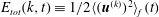 $E_{tot}(k,t)\equiv 1/2\langle (\boldsymbol{u}^{(k)})^{2}\rangle _{f}(t)$
and
$E_{tot}(k,t)\equiv 1/2\langle (\boldsymbol{u}^{(k)})^{2}\rangle _{f}(t)$
and
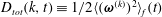 $D_{tot}(k,t)\equiv 1/2\langle (\unicode[STIX]{x1D74E}^{(k)})^{2}\rangle _{f}(t)$
, where
$D_{tot}(k,t)\equiv 1/2\langle (\unicode[STIX]{x1D74E}^{(k)})^{2}\rangle _{f}(t)$
, where
 $E_{tot}(k,t)=[E_{r}+E_{\unicode[STIX]{x1D703}}+E_{z}](k,t)$
and
$E_{tot}(k,t)=[E_{r}+E_{\unicode[STIX]{x1D703}}+E_{z}](k,t)$
and
 $D_{tot}(k,t)=[D_{r}+D_{\unicode[STIX]{x1D703}}+D_{z}](k,t)$
.
$D_{tot}(k,t)=[D_{r}+D_{\unicode[STIX]{x1D703}}+D_{z}](k,t)$
.

Figure 12. Time evolutions of the directionally decomposed energy spectra and the non-decomposed energy spectrum. The blue, green, red and black lines correspond to
 $E_{r}(k=6,t)$
,
$E_{r}(k=6,t)$
,
 $E_{\unicode[STIX]{x1D703}}(k=6,t)$
,
$E_{\unicode[STIX]{x1D703}}(k=6,t)$
,
 $E_{z}(k=6,t)$
and
$E_{z}(k=6,t)$
and
 $E_{tot}(k=6,t)$
, respectively.
$E_{tot}(k=6,t)$
, respectively.

Figure 13. Linear-log plots of temporal standard deviations of directionally decomposed and non-decomposed spectra. Circles, triangles, squares and diamonds correspond respectively to (a)
 $E_{r}$
,
$E_{r}$
,
 $E_{\unicode[STIX]{x1D703}}$
,
$E_{\unicode[STIX]{x1D703}}$
,
 $E_{z}$
,
$E_{z}$
,
 $E_{tot}$
and (b)
$E_{tot}$
and (b)
 $D_{r}$
,
$D_{r}$
,
 $D_{\unicode[STIX]{x1D703}}$
,
$D_{\unicode[STIX]{x1D703}}$
,
 $D_{z}$
,
$D_{z}$
,
 $D_{tot}$
which are defined in § 4. The 4th and 6th modes are highlighted by the black dashed vertical lines. The red and blue dash-dotted vertical lines indicate the wavenumbers
$D_{tot}$
which are defined in § 4. The 4th and 6th modes are highlighted by the black dashed vertical lines. The red and blue dash-dotted vertical lines indicate the wavenumbers
 $k_{L}$
and
$k_{L}$
and
 $k_{\unicode[STIX]{x1D706}}$
, respectively.
$k_{\unicode[STIX]{x1D706}}$
, respectively.
To demonstrate an example of the decomposition we plot, in figure 12, the time evolutions of three directionally decomposed energy spectra and non-decomposed energy spectrum at
 $k=6$
. The time-averaged circumferential energy spectrum
$k=6$
. The time-averaged circumferential energy spectrum
 $\langle E_{\unicode[STIX]{x1D703}}\rangle (k=6)$
is more than four times as large as
$\langle E_{\unicode[STIX]{x1D703}}\rangle (k=6)$
is more than four times as large as
 $\langle E_{r}\rangle (k=6)$
and
$\langle E_{r}\rangle (k=6)$
and
 $\langle E_{z}\rangle (k=6)$
:
$\langle E_{z}\rangle (k=6)$
:
 $\langle E_{\unicode[STIX]{x1D703}}\rangle (k=6)/\langle E_{r}\rangle (k=6)=5.20$
and
$\langle E_{\unicode[STIX]{x1D703}}\rangle (k=6)/\langle E_{r}\rangle (k=6)=5.20$
and
 $\langle E_{\unicode[STIX]{x1D703}}\rangle (k=6)/\langle E_{z}\rangle (k=6)=4.23$
. The amplitude of temporal fluctuation of
$\langle E_{\unicode[STIX]{x1D703}}\rangle (k=6)/\langle E_{z}\rangle (k=6)=4.23$
. The amplitude of temporal fluctuation of
 $E_{\unicode[STIX]{x1D703}}(k=6,t)$
around its temporal mean is much larger than those of
$E_{\unicode[STIX]{x1D703}}(k=6,t)$
around its temporal mean is much larger than those of
 $E_{r}(k=6,t)$
and
$E_{r}(k=6,t)$
and
 $E_{z}(k=6,t)$
; the temporal standard deviation of
$E_{z}(k=6,t)$
; the temporal standard deviation of
 $E_{\unicode[STIX]{x1D703}}(k=6,t)$
is larger than those of
$E_{\unicode[STIX]{x1D703}}(k=6,t)$
is larger than those of
 $E_{r}(k=6,t)$
and
$E_{r}(k=6,t)$
and
 $E_{z}(k=6,t)$
by a factor of 6.26 and 4.93, respectively (i.e.
$E_{z}(k=6,t)$
by a factor of 6.26 and 4.93, respectively (i.e.
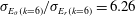 $\unicode[STIX]{x1D70E}_{E_{\unicode[STIX]{x1D703}}(k=6)}/\unicode[STIX]{x1D70E}_{E_{r}(k=6)}=6.26$
and
$\unicode[STIX]{x1D70E}_{E_{\unicode[STIX]{x1D703}}(k=6)}/\unicode[STIX]{x1D70E}_{E_{r}(k=6)}=6.26$
and
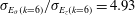 $\unicode[STIX]{x1D70E}_{E_{\unicode[STIX]{x1D703}}(k=6)}/\unicode[STIX]{x1D70E}_{E_{z}(k=6)}=4.93$
). This means that the temporal variation of
$\unicode[STIX]{x1D70E}_{E_{\unicode[STIX]{x1D703}}(k=6)}/\unicode[STIX]{x1D70E}_{E_{z}(k=6)}=4.93$
). This means that the temporal variation of
 $E_{tot}(k=6,t)$
is mainly reflected by that of large-scale swirling flow around the central axis of the larger-scale vortex.
$E_{tot}(k=6,t)$
is mainly reflected by that of large-scale swirling flow around the central axis of the larger-scale vortex.
Besides the 6th mode, let us examine anisotropic fluctuations of other modes. Figure 13(a) shows the temporal standard deviations of the directionally decomposed energy spectra
 $E_{r}(k,t)$
,
$E_{r}(k,t)$
,
 $E_{\unicode[STIX]{x1D703}}(k,t)$
and
$E_{\unicode[STIX]{x1D703}}(k,t)$
and
 $E_{z}(k,t)$
, and the non-decomposed energy spectrum
$E_{z}(k,t)$
, and the non-decomposed energy spectrum
 $E_{tot}(k,t)$
, as a function of wavenumber. All the lower modes than the 3rd mode are not shown because Kida’s high symmetry (Kida Reference Kida1985) sets their values to zero. It is clear that temporal fluctuations of spectra are strongly directional at low Fourier modes, including the 6th mode, such that the circumferential component is dominant (see figure 13
a). For the 4th mode, for instance, we verify that
$E_{tot}(k,t)$
, as a function of wavenumber. All the lower modes than the 3rd mode are not shown because Kida’s high symmetry (Kida Reference Kida1985) sets their values to zero. It is clear that temporal fluctuations of spectra are strongly directional at low Fourier modes, including the 6th mode, such that the circumferential component is dominant (see figure 13
a). For the 4th mode, for instance, we verify that
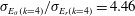 $\unicode[STIX]{x1D70E}_{E_{\unicode[STIX]{x1D703}}(k=4)}/\unicode[STIX]{x1D70E}_{E_{r}(k=4)}=4.46$
and
$\unicode[STIX]{x1D70E}_{E_{\unicode[STIX]{x1D703}}(k=4)}/\unicode[STIX]{x1D70E}_{E_{r}(k=4)}=4.46$
and
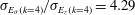 $\unicode[STIX]{x1D70E}_{E_{\unicode[STIX]{x1D703}}(k=4)}/\unicode[STIX]{x1D70E}_{E_{z}(k=4)}=4.29$
.
$\unicode[STIX]{x1D70E}_{E_{\unicode[STIX]{x1D703}}(k=4)}/\unicode[STIX]{x1D70E}_{E_{z}(k=4)}=4.29$
.
Figure 13(b) shows the temporal standard deviations of
 $D_{r}(k,t)$
,
$D_{r}(k,t)$
,
 $D_{\unicode[STIX]{x1D703}}(k,t)$
,
$D_{\unicode[STIX]{x1D703}}(k,t)$
,
 $D_{z}(k,t)$
, and
$D_{z}(k,t)$
, and
 $D_{tot}(k,t)$
. The temporal standard deviation of
$D_{tot}(k,t)$
. The temporal standard deviation of
 $D_{z}(k,t)$
is larger than those of
$D_{z}(k,t)$
is larger than those of
 $D_{r}(k,t)$
and
$D_{r}(k,t)$
and
 $D_{\unicode[STIX]{x1D703}}(k,t)$
at low modes (
$D_{\unicode[STIX]{x1D703}}(k,t)$
at low modes (
 $4\leqslant k\leqslant k_{L}$
) with the exception of the 7th mode. However, as the mode is increased from the 3rd mode, the temporal standard deviation of
$4\leqslant k\leqslant k_{L}$
) with the exception of the 7th mode. However, as the mode is increased from the 3rd mode, the temporal standard deviation of
 $D_{\unicode[STIX]{x1D703}}(k,t)$
is increasing significantly; for several moderate modes comparable to
$D_{\unicode[STIX]{x1D703}}(k,t)$
is increasing significantly; for several moderate modes comparable to
 $k_{\unicode[STIX]{x1D706}}$
, it is much larger than that of
$k_{\unicode[STIX]{x1D706}}$
, it is much larger than that of
 $D_{z}(k,t)$
. This demonstrates that, at moderate wavenumbers, the temporal fluctuation of
$D_{z}(k,t)$
. This demonstrates that, at moderate wavenumbers, the temporal fluctuation of
 $D_{tot}(k,t)$
is strongly affected by the events of generation, circumferential vortex stretching and dissipation of the smaller-scale vortices.
$D_{tot}(k,t)$
is strongly affected by the events of generation, circumferential vortex stretching and dissipation of the smaller-scale vortices.
4.3 Spatial distribution of intense anisotropic fluctuations
As the global fluctuations have been analysed into different directions and scales, we next seek for the spatial origin of intense fluctuations of quantities based on multi-scale and multi-orientation decomposition. In order to do this, we extract turbulent spatial fluctuations of different scales from multi-scale turbulent flow fields by using a bandpass-filtering approach which has been exploited in the literature (Leung et al.
Reference Leung, Swaminathan and Davidson2012; Cardesa, Vela-Martín & Jiménez Reference Cardesa, Vela-Martín and Jiménez2017; Goto et al.
Reference Goto, Saito and Kawahara2017). For the filter, we employ a sharp-cutoff bandpass filter since the Fourier mode decomposition has been used in our preceding discussion. We compute the bandpass-filtered vorticity field
 $\widehat{\unicode[STIX]{x1D74E}}(\boldsymbol{x},t)$
in physical space by applying the sharp-cutoff bandpass filter
$\widehat{\unicode[STIX]{x1D74E}}(\boldsymbol{x},t)$
in physical space by applying the sharp-cutoff bandpass filter
 $G(\boldsymbol{k})$
to the vorticity field in Fourier space as
$G(\boldsymbol{k})$
to the vorticity field in Fourier space as
 $$\begin{eqnarray}\displaystyle \widehat{\unicode[STIX]{x1D74E}}(\boldsymbol{x},t)=\mathop{\sum }_{\boldsymbol{k}}G(\boldsymbol{k})\widetilde{\unicode[STIX]{x1D74E}}(\boldsymbol{k},t)\text{e}^{\text{i}\boldsymbol{k}\boldsymbol{\cdot }\boldsymbol{x}}, & & \displaystyle\end{eqnarray}$$
where
 $$\begin{eqnarray}\displaystyle G(\boldsymbol{k}) & = & \displaystyle 1,\quad \text{for}~k_{low}-{\textstyle \frac{1}{2}}\leqslant |\boldsymbol{k}|<k_{high}+{\textstyle \frac{1}{2}},\nonumber\\ \displaystyle & = & \displaystyle 0,\quad \text{otherwise},\end{eqnarray}$$
and
 $k_{low}$
and
$k_{low}$
and
 $k_{high}$
are the lower and higher cutoff wavenumbers, respectively. Considering the dependency of anisotropic enstrophy fluctuation on different modes (figure 13
b), we use three wavenumber ranges: [R1]
$k_{high}$
are the lower and higher cutoff wavenumbers, respectively. Considering the dependency of anisotropic enstrophy fluctuation on different modes (figure 13
b), we use three wavenumber ranges: [R1]
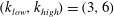 $(k_{low},k_{high})=(3,6)$
; [R2]
$(k_{low},k_{high})=(3,6)$
; [R2]
 $(k_{low},k_{high})=(9,16)$
; [R3]
$(k_{low},k_{high})=(9,16)$
; [R3]
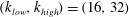 $(k_{low},k_{high})=(16,32)$
. Here, we set the range [R1] to include the fixed modes and intensely fluctuating modes of circumferential velocity and axial vorticity, which are 4th and 6th modes, the range [R2] to include the modes showing relatively strong fluctuation in circumferential enstrophy spectrum seen in figure 13(b), and the range [R3] to have dissipative small scales. Using (3.1), the filtered vorticity obtained is finally decomposed into the filtered radial vorticity
$(k_{low},k_{high})=(16,32)$
. Here, we set the range [R1] to include the fixed modes and intensely fluctuating modes of circumferential velocity and axial vorticity, which are 4th and 6th modes, the range [R2] to include the modes showing relatively strong fluctuation in circumferential enstrophy spectrum seen in figure 13(b), and the range [R3] to have dissipative small scales. Using (3.1), the filtered vorticity obtained is finally decomposed into the filtered radial vorticity
 $\widehat{\unicode[STIX]{x1D714}}_{r}(\boldsymbol{x},t)$
, the filtered circumferential vorticity
$\widehat{\unicode[STIX]{x1D714}}_{r}(\boldsymbol{x},t)$
, the filtered circumferential vorticity
 $\widehat{\unicode[STIX]{x1D714}}_{\unicode[STIX]{x1D703}}(\boldsymbol{x},t)$
and the filtered axial vorticity
$\widehat{\unicode[STIX]{x1D714}}_{\unicode[STIX]{x1D703}}(\boldsymbol{x},t)$
and the filtered axial vorticity
 $\widehat{\unicode[STIX]{x1D714}}_{z}(\boldsymbol{x},t)$
.
$\widehat{\unicode[STIX]{x1D714}}_{z}(\boldsymbol{x},t)$
.
Because of Kida’s high symmetry (Kida Reference Kida1985), which fixes in space the central axes of larger-scale vortices, strongly fluctuating regions are spatially localised inside a fundamental box. In order to detect such regions, we compute the temporal standard deviation field
 $\unicode[STIX]{x1D6F4}(\boldsymbol{x};A)$
of scalar quantity
$\unicode[STIX]{x1D6F4}(\boldsymbol{x};A)$
of scalar quantity
 $A$
, which is defined as
$A$
, which is defined as
 $$\begin{eqnarray}\displaystyle \unicode[STIX]{x1D6F4}(\boldsymbol{x};A)=\sqrt{\frac{1}{T_{p}}\int _{0}^{T_{p}}(A(\boldsymbol{x},t)-\langle A\rangle (\boldsymbol{x}))^{2}\,\text{d}t}, & & \displaystyle\end{eqnarray}$$
where
 $T_{p}$
is set to the time period of the period-5 motion.
$T_{p}$
is set to the time period of the period-5 motion.

Figure 14. Visualisations of temporal standard deviation fields of (a) filtered axial vorticity
 $\widehat{\unicode[STIX]{x1D714}}_{z}$
, (b) filtered radial vorticity
$\widehat{\unicode[STIX]{x1D714}}_{z}$
, (b) filtered radial vorticity
 $\widehat{\unicode[STIX]{x1D714}}_{r}$
and (c) filtered circumferential vorticity
$\widehat{\unicode[STIX]{x1D714}}_{r}$
and (c) filtered circumferential vorticity
 $\widehat{\unicode[STIX]{x1D714}}_{\unicode[STIX]{x1D703}}$
. Red, blue and green isosurfaces correspond respectively to the filtered vorticity obtained with the ranges [R1]
$\widehat{\unicode[STIX]{x1D714}}_{\unicode[STIX]{x1D703}}$
. Red, blue and green isosurfaces correspond respectively to the filtered vorticity obtained with the ranges [R1]
 $(k_{low},k_{high})=(3,6)$
, [R2]
$(k_{low},k_{high})=(3,6)$
, [R2]
 $(9,16)$
and [R3]
$(9,16)$
and [R3]
 $(16,32)$
, which are explained in § 4.3. (a) Red,
$(16,32)$
, which are explained in § 4.3. (a) Red,
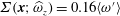 $\unicode[STIX]{x1D6F4}(\boldsymbol{x};\widehat{\unicode[STIX]{x1D714}}_{z})=0.16\langle \unicode[STIX]{x1D714}^{\prime }\rangle$
; blue, green,
$\unicode[STIX]{x1D6F4}(\boldsymbol{x};\widehat{\unicode[STIX]{x1D714}}_{z})=0.16\langle \unicode[STIX]{x1D714}^{\prime }\rangle$
; blue, green,
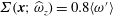 $\unicode[STIX]{x1D6F4}(\boldsymbol{x};\widehat{\unicode[STIX]{x1D714}}_{z})=0.8\langle \unicode[STIX]{x1D714}^{\prime }\rangle$
. (b) Red,
$\unicode[STIX]{x1D6F4}(\boldsymbol{x};\widehat{\unicode[STIX]{x1D714}}_{z})=0.8\langle \unicode[STIX]{x1D714}^{\prime }\rangle$
. (b) Red,
 $\unicode[STIX]{x1D6F4}(\boldsymbol{x};\widehat{\unicode[STIX]{x1D714}}_{r})=0.16\langle \unicode[STIX]{x1D714}^{\prime }\rangle$
; blue, green,
$\unicode[STIX]{x1D6F4}(\boldsymbol{x};\widehat{\unicode[STIX]{x1D714}}_{r})=0.16\langle \unicode[STIX]{x1D714}^{\prime }\rangle$
; blue, green,
 $\unicode[STIX]{x1D6F4}(\boldsymbol{x};\widehat{\unicode[STIX]{x1D714}}_{r})=0.8\langle \unicode[STIX]{x1D714}^{\prime }\rangle$
. (c) Red,
$\unicode[STIX]{x1D6F4}(\boldsymbol{x};\widehat{\unicode[STIX]{x1D714}}_{r})=0.8\langle \unicode[STIX]{x1D714}^{\prime }\rangle$
. (c) Red,
 $\unicode[STIX]{x1D6F4}(\boldsymbol{x};\widehat{\unicode[STIX]{x1D714}}_{\unicode[STIX]{x1D703}})=0.2\langle \unicode[STIX]{x1D714}^{\prime }\rangle$
; blue, green,
$\unicode[STIX]{x1D6F4}(\boldsymbol{x};\widehat{\unicode[STIX]{x1D714}}_{\unicode[STIX]{x1D703}})=0.2\langle \unicode[STIX]{x1D714}^{\prime }\rangle$
; blue, green,
 $\unicode[STIX]{x1D6F4}(\boldsymbol{x};\widehat{\unicode[STIX]{x1D714}}_{\unicode[STIX]{x1D703}})=\langle \unicode[STIX]{x1D714}^{\prime }\rangle$
.
$\unicode[STIX]{x1D6F4}(\boldsymbol{x};\widehat{\unicode[STIX]{x1D714}}_{\unicode[STIX]{x1D703}})=\langle \unicode[STIX]{x1D714}^{\prime }\rangle$
.
Figure 14(a) shows the isosurfaces of large values of
 $\unicode[STIX]{x1D6F4}(\boldsymbol{x};\hat{\unicode[STIX]{x1D714}}_{z})$
. As for the wavenumber range [R1], the isosurfaces which demonstrate the intensely fluctuating regions of filtered axial vorticity are found on the diagonal, i.e. the central axis of larger-scale vortex. Taking into account the fact that temporal fluctuation of
$\unicode[STIX]{x1D6F4}(\boldsymbol{x};\hat{\unicode[STIX]{x1D714}}_{z})$
. As for the wavenumber range [R1], the isosurfaces which demonstrate the intensely fluctuating regions of filtered axial vorticity are found on the diagonal, i.e. the central axis of larger-scale vortex. Taking into account the fact that temporal fluctuation of
 $D_{z}(k=6,t)$
is much larger than those of
$D_{z}(k=6,t)$
is much larger than those of
 $D_{r}(k=6,t)$
and
$D_{r}(k=6,t)$
and
 $D_{\unicode[STIX]{x1D703}}(k=6,t)$
, the spatial origin of excitation of lower modes is considered to be the locations where the isosurfaces are detected. Crucially, even for the filtered axial vorticity obtained with higher wavenumber ranges [R2] and [R3] some isosurfaces of the high values which exhibit strongly fluctuating regions are observed on the diagonal, even in the central region of the fundamental box. The observed regions are associated with axial stretching and compression dynamics by the nonlinear axial waves, which will appear in the next section.
$D_{\unicode[STIX]{x1D703}}(k=6,t)$
, the spatial origin of excitation of lower modes is considered to be the locations where the isosurfaces are detected. Crucially, even for the filtered axial vorticity obtained with higher wavenumber ranges [R2] and [R3] some isosurfaces of the high values which exhibit strongly fluctuating regions are observed on the diagonal, even in the central region of the fundamental box. The observed regions are associated with axial stretching and compression dynamics by the nonlinear axial waves, which will appear in the next section.
Figures 14(b) and 14(c) demonstrate the temporal standard deviation fields
 $\unicode[STIX]{x1D6F4}(\boldsymbol{x};\hat{\unicode[STIX]{x1D714}}_{r})$
and
$\unicode[STIX]{x1D6F4}(\boldsymbol{x};\hat{\unicode[STIX]{x1D714}}_{r})$
and
 $\unicode[STIX]{x1D6F4}(\boldsymbol{x};\hat{\unicode[STIX]{x1D714}}_{\unicode[STIX]{x1D703}})$
, respectively. It is found in the field of
$\unicode[STIX]{x1D6F4}(\boldsymbol{x};\hat{\unicode[STIX]{x1D714}}_{\unicode[STIX]{x1D703}})$
, respectively. It is found in the field of
 $\unicode[STIX]{x1D6F4}(\boldsymbol{x};\hat{\unicode[STIX]{x1D714}}_{r})$
(figure 14
b) that, unlike
$\unicode[STIX]{x1D6F4}(\boldsymbol{x};\hat{\unicode[STIX]{x1D714}}_{r})$
(figure 14
b) that, unlike
 $\unicode[STIX]{x1D6F4}(\boldsymbol{x};\hat{\unicode[STIX]{x1D714}}_{z})$
, none of the isosurfaces appears on the diagonal. For
$\unicode[STIX]{x1D6F4}(\boldsymbol{x};\hat{\unicode[STIX]{x1D714}}_{z})$
, none of the isosurfaces appears on the diagonal. For
 $\unicode[STIX]{x1D6F4}(\boldsymbol{x};\hat{\unicode[STIX]{x1D714}}_{\unicode[STIX]{x1D703}})$
, on the other hand, some isosurfaces appear on the diagonal with the ranges [R2] and [R3] (figure 14
c). This result suggests that, since the smaller-scale vortices own strong circumferential vorticity, there would be significant dynamical interactions between the axial waves and smaller-scale vortices which induce axial flows on the diagonal. This dynamical interaction will be discussed in § 5.2.
$\unicode[STIX]{x1D6F4}(\boldsymbol{x};\hat{\unicode[STIX]{x1D714}}_{\unicode[STIX]{x1D703}})$
, on the other hand, some isosurfaces appear on the diagonal with the ranges [R2] and [R3] (figure 14
c). This result suggests that, since the smaller-scale vortices own strong circumferential vorticity, there would be significant dynamical interactions between the axial waves and smaller-scale vortices which induce axial flows on the diagonal. This dynamical interaction will be discussed in § 5.2.
5 Large-amplitude oscillation in forced high-symmetric turbulence
5.1 Large-amplitude axial waves on larger-scale vortices
In § 4.1, we have detected the intense cyclic forward energy transfer events in the period-5 motion, which are caused after excitations of the 6th mode. We have also found that intensely fluctuating regions of bandpass-filtered axial vorticity obtained with the low wavenumber range [R1] including the wavenumber
 $k=6$
are located on the central axis of the larger-scale vortex (§ 4.3). Based on these results, a question arises: What physical mechanism causes excitations of the key mode, i.e. the 6th mode? This question will be tackled by investigating nonlinear axial waves on the larger-scale vortices. We will demonstrate that the large-amplitude oscillations of the larger-scale vortices are caused with the aid of the nonlinear axial waves, which are excited by the dynamical effect of smaller-scale vortices. Such a sustenance mechanism can be described in terms of supportive dynamical interactions between the larger-scale and smaller-scale vortices, which will be schematically summarised in a cycle diagram (see figure 20). It is reminiscent of the regeneration cycle of turbulent structures in wall-bounded shear flows (Hamilton et al.
Reference Hamilton, Kim and Waleffe1995; Waleffe Reference Waleffe1997) and transitional flows (Shimizu & Kida Reference Shimizu and Kida2009).
$k=6$
are located on the central axis of the larger-scale vortex (§ 4.3). Based on these results, a question arises: What physical mechanism causes excitations of the key mode, i.e. the 6th mode? This question will be tackled by investigating nonlinear axial waves on the larger-scale vortices. We will demonstrate that the large-amplitude oscillations of the larger-scale vortices are caused with the aid of the nonlinear axial waves, which are excited by the dynamical effect of smaller-scale vortices. Such a sustenance mechanism can be described in terms of supportive dynamical interactions between the larger-scale and smaller-scale vortices, which will be schematically summarised in a cycle diagram (see figure 20). It is reminiscent of the regeneration cycle of turbulent structures in wall-bounded shear flows (Hamilton et al.
Reference Hamilton, Kim and Waleffe1995; Waleffe Reference Waleffe1997) and transitional flows (Shimizu & Kida Reference Shimizu and Kida2009).
We emphasise that nonlinear axial waves on larger-scale vortices are essential in the cyclic process. The larger-scale vortices are the largest structures in high-symmetric turbulence. Since there is no larger-scale strain field which gives rise to global stretching or compression of the larger-scale vortices, they should be locally stretched or compressed through nonlinear axial waves to oscillate. We will therefore pay attention to axial motions along the central axes of the larger-scale vortices. In order to clarify this oscillation mechanism, we shall proceed with our discussion based on the following perspectives: (i) local vortex stretching and compression along the central axes of the larger-scale vortices and (ii) dynamical feedbacks from smaller-scale vortices. To begin with, we shall confirm the axial waves.

Figure 15. Time evolutions of physical quantities on the diagonal line of the fundamental box (
 $0\leqslant x_{1},x_{2},x_{3}\leqslant \unicode[STIX]{x03C0}/2$
) for the period-5 motion. Contour values denote (a) axial velocity
$0\leqslant x_{1},x_{2},x_{3}\leqslant \unicode[STIX]{x03C0}/2$
) for the period-5 motion. Contour values denote (a) axial velocity
 $u_{z}$
, (b) axial vorticity
$u_{z}$
, (b) axial vorticity
 $\unicode[STIX]{x1D714}_{z}$
, (c) axial vorticity stretching rate
$\unicode[STIX]{x1D714}_{z}$
, (c) axial vorticity stretching rate
 $\unicode[STIX]{x1D714}_{z}(\unicode[STIX]{x2202}u_{z}/\unicode[STIX]{x2202}z)$
and (d) pressure
$\unicode[STIX]{x1D714}_{z}(\unicode[STIX]{x2202}u_{z}/\unicode[STIX]{x2202}z)$
and (d) pressure
 $p$
. Horizontal and vertical axes represent the time and coordinates on the diagonal line (
$p$
. Horizontal and vertical axes represent the time and coordinates on the diagonal line (
 $0\leqslant z/(\sqrt{3}\unicode[STIX]{x03C0}/2)\leqslant 1$
).
$0\leqslant z/(\sqrt{3}\unicode[STIX]{x03C0}/2)\leqslant 1$
).
 $z=0$
and
$z=0$
and
 $z=\sqrt{3}\unicode[STIX]{x03C0}/2$
correspond to the origin O and point A, respectively. The thick and thin dashed lines represent times when
$z=\sqrt{3}\unicode[STIX]{x03C0}/2$
correspond to the origin O and point A, respectively. The thick and thin dashed lines represent times when
 $\langle u_{\unicode[STIX]{x1D703}}^{2}\rangle _{f}$
attains a local maximum and when
$\langle u_{\unicode[STIX]{x1D703}}^{2}\rangle _{f}$
attains a local maximum and when
 $E(k=6,t)$
attains a local maximum, respectively. (b) The filled (open) inverted triangles indicate the local maximum (local minimum) of axial vorticity along the diagonal in the range
$E(k=6,t)$
attains a local maximum, respectively. (b) The filled (open) inverted triangles indicate the local maximum (local minimum) of axial vorticity along the diagonal in the range
 $0\leqslant z/(\sqrt{3}\unicode[STIX]{x03C0}/2)\leqslant 0.3$
. The filled (open) triangles indicate the local maximum (local minimum) of axial vorticity along the diagonal in the range
$0\leqslant z/(\sqrt{3}\unicode[STIX]{x03C0}/2)\leqslant 0.3$
. The filled (open) triangles indicate the local maximum (local minimum) of axial vorticity along the diagonal in the range
 $0.6\leqslant z/(\sqrt{3}\unicode[STIX]{x03C0}/2)\leqslant 1$
.
$0.6\leqslant z/(\sqrt{3}\unicode[STIX]{x03C0}/2)\leqslant 1$
.
We turn to figure 15 which shows the time evolution of axial motions along the central axis of the larger-scale vortex in the fundamental box (
 $0\leqslant x_{1},x_{2},x_{3}\leqslant \unicode[STIX]{x03C0}/2$
) for the period-5 motion. Within this time period (
$0\leqslant x_{1},x_{2},x_{3}\leqslant \unicode[STIX]{x03C0}/2$
) for the period-5 motion. Within this time period (
 $0\leqslant t/T\leqslant 9.85$
), all the quantities shown in the figure (axial velocity
$0\leqslant t/T\leqslant 9.85$
), all the quantities shown in the figure (axial velocity
 $u_{z}$
, axial vorticity
$u_{z}$
, axial vorticity
 $\unicode[STIX]{x1D714}_{z}$
, axial vorticity stretching rate
$\unicode[STIX]{x1D714}_{z}$
, axial vorticity stretching rate
 $\unicode[STIX]{x1D714}_{z}(\unicode[STIX]{x2202}u_{z}/\unicode[STIX]{x2202}z)$
and pressure
$\unicode[STIX]{x1D714}_{z}(\unicode[STIX]{x2202}u_{z}/\unicode[STIX]{x2202}z)$
and pressure
 $p$
) fluctuate cyclically, with large amplitude, five times. Along the central axis, the axial vorticity
$p$
) fluctuate cyclically, with large amplitude, five times. Along the central axis, the axial vorticity
 $\unicode[STIX]{x1D714}_{z}$
is not homogeneous; the area of lower vorticity (local lower-speed rotational motion) and that of higher vorticity (local higher-speed rotational motion) are alternately aligned. An important observation in figure 15 is that the axial waves on the larger-scale vortex include a standing wave pattern and two travelling wave patterns, depending on the axial position
$\unicode[STIX]{x1D714}_{z}$
is not homogeneous; the area of lower vorticity (local lower-speed rotational motion) and that of higher vorticity (local higher-speed rotational motion) are alternately aligned. An important observation in figure 15 is that the axial waves on the larger-scale vortex include a standing wave pattern and two travelling wave patterns, depending on the axial position
 $z$
(
$z$
(
 $0\leqslant z/(\sqrt{3}\unicode[STIX]{x03C0}/2)\leqslant 1$
;
$0\leqslant z/(\sqrt{3}\unicode[STIX]{x03C0}/2)\leqslant 1$
;
 $z=0$
(or
$z=0$
(or
 $z=\sqrt{3}\unicode[STIX]{x03C0}/2$
) represents the origin O (or the point A)). For convenience, we hereinafter refer to the range
$z=\sqrt{3}\unicode[STIX]{x03C0}/2$
) represents the origin O (or the point A)). For convenience, we hereinafter refer to the range
 $0.3\leqslant z/(\sqrt{3}\unicode[STIX]{x03C0}/2)\leqslant 0.6$
as the inner region, where a standing wave pattern is observed, and the ranges
$0.3\leqslant z/(\sqrt{3}\unicode[STIX]{x03C0}/2)\leqslant 0.6$
as the inner region, where a standing wave pattern is observed, and the ranges
 $0\leqslant z/(\sqrt{3}\unicode[STIX]{x03C0}/2)\leqslant 0.3$
and
$0\leqslant z/(\sqrt{3}\unicode[STIX]{x03C0}/2)\leqslant 0.3$
and
 $0.6\leqslant z/(\sqrt{3}\unicode[STIX]{x03C0}/2)\leqslant 1$
, where travelling wave patterns are observed, as the outer-O region and the outer-A region, respectively.
$0.6\leqslant z/(\sqrt{3}\unicode[STIX]{x03C0}/2)\leqslant 1$
, where travelling wave patterns are observed, as the outer-O region and the outer-A region, respectively.
The standing wave pattern is observed in figure 15(b) such that the time evolution of
 $\unicode[STIX]{x1D714}_{z}$
in the range
$\unicode[STIX]{x1D714}_{z}$
in the range
 $0.3\leqslant z/(\sqrt{3}\unicode[STIX]{x03C0}/2)\leqslant 0.6$
shows temporal alternations of low and high axial vorticity. The areas of low vorticity have often been called ‘bubbles’ in the literature (e.g. Leibovich & Kribus Reference Leibovich and Kribus1990; Melander & Hussain Reference Melander and Hussain1994; Verzicco et al.
Reference Verzicco, Jiménez and Orlandi1995); they are considered as a consequence of local axial vorticity compression in a longitudinal wave along the central axis of a columnar vortex. They are not permanent flow structures (except in stationary flows or equilibrium solutions), but decay because of local axial vorticity stretching which subsequently happens. Such axial vorticity compression and stretching are caused by the axial flows accelerated by the axial pressure gradient from the areas of lower axial vorticity, which nearly corresponds to the higher-pressure areas, to those of higher axial vorticity, which nearly corresponds to the lower-pressure areas. The reason why the areas of lower (or higher) axial vorticity nearly correspond to those of higher (or lower) pressure is due to the centrifugal force: If rotational motion around the central axis of a larger-scale vortex gets faster (i.e. the axial vorticity
$0.3\leqslant z/(\sqrt{3}\unicode[STIX]{x03C0}/2)\leqslant 0.6$
shows temporal alternations of low and high axial vorticity. The areas of low vorticity have often been called ‘bubbles’ in the literature (e.g. Leibovich & Kribus Reference Leibovich and Kribus1990; Melander & Hussain Reference Melander and Hussain1994; Verzicco et al.
Reference Verzicco, Jiménez and Orlandi1995); they are considered as a consequence of local axial vorticity compression in a longitudinal wave along the central axis of a columnar vortex. They are not permanent flow structures (except in stationary flows or equilibrium solutions), but decay because of local axial vorticity stretching which subsequently happens. Such axial vorticity compression and stretching are caused by the axial flows accelerated by the axial pressure gradient from the areas of lower axial vorticity, which nearly corresponds to the higher-pressure areas, to those of higher axial vorticity, which nearly corresponds to the lower-pressure areas. The reason why the areas of lower (or higher) axial vorticity nearly correspond to those of higher (or lower) pressure is due to the centrifugal force: If rotational motion around the central axis of a larger-scale vortex gets faster (i.e. the axial vorticity
 $\unicode[STIX]{x1D714}_{z}$
becomes larger), then shortly pressure on the axis gets lower to counter-balance the centrifugal force because of strong swirling motion induced by the rotational motion. Because of the axial pressure gradient and the centrifugal force, axial inhomogeneity in axial vorticity and pressure is a driving source of axial waves. Alternative explanations of axisymmetric standing waves can be found in the literature (Melander & Hussain Reference Melander and Hussain1994; Fabre et al.
Reference Fabre, Sipp and Jacquin2006).
$\unicode[STIX]{x1D714}_{z}$
becomes larger), then shortly pressure on the axis gets lower to counter-balance the centrifugal force because of strong swirling motion induced by the rotational motion. Because of the axial pressure gradient and the centrifugal force, axial inhomogeneity in axial vorticity and pressure is a driving source of axial waves. Alternative explanations of axisymmetric standing waves can be found in the literature (Melander & Hussain Reference Melander and Hussain1994; Fabre et al.
Reference Fabre, Sipp and Jacquin2006).

Figure 16. Similar to figure 15, but focusing on the time period (
 $6.27\leqslant t/T\leqslant 9.18$
) shown in figure 7. The thick dashed lines correspond to times 1–7 shown in figure 7. The thin dashed line denotes the time when
$6.27\leqslant t/T\leqslant 9.18$
) shown in figure 7. The thick dashed lines correspond to times 1–7 shown in figure 7. The thin dashed line denotes the time when
 $E(k=6,t)$
is maximal (
$E(k=6,t)$
is maximal (
 $t=7.75T$
). The double triangle and double inverted triangle indicate the locations of local minimum pressure at
$t=7.75T$
). The double triangle and double inverted triangle indicate the locations of local minimum pressure at
 $t=t_{4}$
in the outer-A region and inner region, respectively. The double circle indicates the zero-crossing point of axial velocity at
$t=t_{4}$
in the outer-A region and inner region, respectively. The double circle indicates the zero-crossing point of axial velocity at
 $t=t_{5}$
.
$t=t_{5}$
.

Figure 17. Snapshots of the flow fields in the fundamental box (
 $0\leqslant x_{1},x_{2},x_{3}\leqslant \unicode[STIX]{x03C0}/2$
), taken at the corresponding times in figure 7: (a)
$0\leqslant x_{1},x_{2},x_{3}\leqslant \unicode[STIX]{x03C0}/2$
), taken at the corresponding times in figure 7: (a)
 $t=t_{1}$
(
$t=t_{1}$
(
 $6.74T$
), (b)
$6.74T$
), (b)
 $t_{2}$
(
$t_{2}$
(
 $7.04T$
), (c)
$7.04T$
), (c)
 $t_{3}$
(
$t_{3}$
(
 $7.40T$
), (d)
$7.40T$
), (d)
 $t_{4}$
(
$t_{4}$
(
 $7.66T$
), (e)
$7.66T$
), (e)
 $t_{5}$
(
$t_{5}$
(
 $8.09T$
), (f)
$8.09T$
), (f)
 $t_{6}$
(
$t_{6}$
(
 $8.38T$
), (g)
$8.38T$
), (g)
 $t_{7}$
(
$t_{7}$
(
 $8.70T$
). The grey, yellow and blue-coloured isosurfaces represent
$8.70T$
). The grey, yellow and blue-coloured isosurfaces represent
 $p/[\unicode[STIX]{x1D70C}\langle u^{\prime }\rangle ^{2}]=-2$
,
$p/[\unicode[STIX]{x1D70C}\langle u^{\prime }\rangle ^{2}]=-2$
,
 $\unicode[STIX]{x1D714}_{z}/\langle \unicode[STIX]{x1D714}^{\prime }\rangle =4.54$
and
$\unicode[STIX]{x1D714}_{z}/\langle \unicode[STIX]{x1D714}^{\prime }\rangle =4.54$
and
 $\unicode[STIX]{x1D714}_{\unicode[STIX]{x1D703}}/\langle \unicode[STIX]{x1D714}^{\prime }\rangle =-4.54$
, respectively. The two-dimensional velocity vectors are shown on the plane including the points O, A and
$\unicode[STIX]{x1D714}_{\unicode[STIX]{x1D703}}/\langle \unicode[STIX]{x1D714}^{\prime }\rangle =-4.54$
, respectively. The two-dimensional velocity vectors are shown on the plane including the points O, A and
 $(0,\unicode[STIX]{x03C0}/2,0)$
. The double triangle and double inverted triangle indicate the locations of local minimum pressure at
$(0,\unicode[STIX]{x03C0}/2,0)$
. The double triangle and double inverted triangle indicate the locations of local minimum pressure at
 $t=t_{4}$
in the outer-A region and inner region, respectively. The double circle indicates the zero-crossing point of axial velocity at
$t=t_{4}$
in the outer-A region and inner region, respectively. The double circle indicates the zero-crossing point of axial velocity at
 $t=t_{5}$
. See the supplementary movie of the corresponding time evolution available at https://doi.org/10.1017/jfm.2019.370.
$t=t_{5}$
. See the supplementary movie of the corresponding time evolution available at https://doi.org/10.1017/jfm.2019.370.

Figure 18. Snapshots of the flow fields in the fundamental box (
 $0\leqslant x_{1},x_{2},x_{3}\leqslant \unicode[STIX]{x03C0}/2$
). They are taken at (a)
$0\leqslant x_{1},x_{2},x_{3}\leqslant \unicode[STIX]{x03C0}/2$
). They are taken at (a)
 $t=t_{1}$
(
$t=t_{1}$
(
 $6.74T$
), (b)
$6.74T$
), (b)
 $t_{2}$
(
$t_{2}$
(
 $7.04T$
), (c)
$7.04T$
), (c)
 $t_{3}$
(
$t_{3}$
(
 $7.40T$
), (d)
$7.40T$
), (d)
 $t_{4}$
(
$t_{4}$
(
 $7.66T$
). The grey, yellow, red and blue-coloured isosurfaces represent
$7.66T$
). The grey, yellow, red and blue-coloured isosurfaces represent
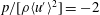 $p/[\unicode[STIX]{x1D70C}\langle u^{\prime }\rangle ^{2}]=-2$
,
$p/[\unicode[STIX]{x1D70C}\langle u^{\prime }\rangle ^{2}]=-2$
,
 $\unicode[STIX]{x1D714}_{z}/\langle \unicode[STIX]{x1D714}^{\prime }\rangle =4.54$
,
$\unicode[STIX]{x1D714}_{z}/\langle \unicode[STIX]{x1D714}^{\prime }\rangle =4.54$
,
 $\unicode[STIX]{x1D714}_{\unicode[STIX]{x1D703}}/\langle \unicode[STIX]{x1D714}^{\prime }\rangle =4.54$
and
$\unicode[STIX]{x1D714}_{\unicode[STIX]{x1D703}}/\langle \unicode[STIX]{x1D714}^{\prime }\rangle =4.54$
and
 $\unicode[STIX]{x1D714}_{\unicode[STIX]{x1D703}}/\langle \unicode[STIX]{x1D714}^{\prime }\rangle =-4.54$
, respectively. The two-dimensional velocity vectors are shown on the plane including the points O, A and
$\unicode[STIX]{x1D714}_{\unicode[STIX]{x1D703}}/\langle \unicode[STIX]{x1D714}^{\prime }\rangle =-4.54$
, respectively. The two-dimensional velocity vectors are shown on the plane including the points O, A and
 $(0,\unicode[STIX]{x03C0}/2,0)$
. The SV-A vortex denoted by the arrow is approaching towards the central axis of larger-scale vortex and induces the strong axial flow (
$(0,\unicode[STIX]{x03C0}/2,0)$
. The SV-A vortex denoted by the arrow is approaching towards the central axis of larger-scale vortex and induces the strong axial flow (
 $u_{z}<0$
).
$u_{z}<0$
).

Figure 19. Similar to figure 16, but the time evolutions of (a) 4th-mode axial vorticity
 $\unicode[STIX]{x1D714}_{z}^{(4)}$
and (b) 6th-mode axial vorticity
$\unicode[STIX]{x1D714}_{z}^{(4)}$
and (b) 6th-mode axial vorticity
 $\unicode[STIX]{x1D714}_{z}^{(6)}$
on the diagonal line of the fundamental box (
$\unicode[STIX]{x1D714}_{z}^{(6)}$
on the diagonal line of the fundamental box (
 $0\leqslant x_{1},x_{2},x_{3}\leqslant \unicode[STIX]{x03C0}/2$
) for the period-5 motion.
$0\leqslant x_{1},x_{2},x_{3}\leqslant \unicode[STIX]{x03C0}/2$
) for the period-5 motion.
The travelling wave pattern is, on the other hand, observed such that the areas of lower and higher vorticity in the range
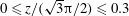 $0\leqslant z/(\sqrt{3}\unicode[STIX]{x03C0}/2)\leqslant 0.3$
(the outer-O region) move towards the origin O; those in
$0\leqslant z/(\sqrt{3}\unicode[STIX]{x03C0}/2)\leqslant 0.3$
(the outer-O region) move towards the origin O; those in
 $0.6\leqslant z/(\sqrt{3}\unicode[STIX]{x03C0}/2)\leqslant 1$
(the outer-A region) move towards the point A. In order to make this point more evident, we plot in figure 15(b) the triangles along the central axis where the local maxima and minima of axial vorticity
$0.6\leqslant z/(\sqrt{3}\unicode[STIX]{x03C0}/2)\leqslant 1$
(the outer-A region) move towards the point A. In order to make this point more evident, we plot in figure 15(b) the triangles along the central axis where the local maxima and minima of axial vorticity
 $\unicode[STIX]{x1D714}_{z}$
are detected. The plot of the filled (open) inverted triangles indicates that the local maximum (local minimum) of axial vorticity propagates towards the origin O, whereas that of the filled (open) triangles indicates that the local maximum (local minimum) of axial vorticity propagates towards the point A.
$\unicode[STIX]{x1D714}_{z}$
are detected. The plot of the filled (open) inverted triangles indicates that the local maximum (local minimum) of axial vorticity propagates towards the origin O, whereas that of the filled (open) triangles indicates that the local maximum (local minimum) of axial vorticity propagates towards the point A.
Here, we shall explain in more detail the travelling wave pattern in the outer-A region within the time period
 $6.27\leqslant t/T\leqslant 9.18$
(see figure 16). In the contour plot of
$6.27\leqslant t/T\leqslant 9.18$
(see figure 16). In the contour plot of
 $\unicode[STIX]{x1D714}_{z}$
(figure 16
b), we observe that the strong axial vorticity region is moving from its onset point towards the endpoint A of the diagonal. Within the shown time period (
$\unicode[STIX]{x1D714}_{z}$
(figure 16
b), we observe that the strong axial vorticity region is moving from its onset point towards the endpoint A of the diagonal. Within the shown time period (
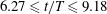 $6.27\leqslant t/T\leqslant 9.18$
), the event of local maximum of axial vorticity propagating towards the point A is observed twice. For the first propagation event, local maximum of axial vorticity attains at
$6.27\leqslant t/T\leqslant 9.18$
), the event of local maximum of axial vorticity propagating towards the point A is observed twice. For the first propagation event, local maximum of axial vorticity attains at
 $(t,z/(\sqrt{3}\unicode[STIX]{x03C0}/2))=(t_{1},0.656)$
,
$(t,z/(\sqrt{3}\unicode[STIX]{x03C0}/2))=(t_{1},0.656)$
,
 $(t_{2},0.758)$
,
$(t_{2},0.758)$
,
 $(t_{3},0.805)$
,
$(t_{3},0.805)$
,
 $(t_{4},0.867)$
,
$(t_{4},0.867)$
,
 $(t_{5},0.914)$
,
$(t_{5},0.914)$
,
 $(t_{6},0.938)$
and
$(t_{6},0.938)$
and
 $(t_{7},0.945)$
, while
$(t_{7},0.945)$
, while
 $(t,z/(\sqrt{3}\unicode[STIX]{x03C0}/2))=(t_{5},0.648)$
,
$(t,z/(\sqrt{3}\unicode[STIX]{x03C0}/2))=(t_{5},0.648)$
,
 $(t_{6},0.712)$
and
$(t_{6},0.712)$
and
 $(t_{7},0.766)$
for the second propagation event. We verify in our flow visualisation (figure 17) that the yellow isosurface of the large value of
$(t_{7},0.766)$
for the second propagation event. We verify in our flow visualisation (figure 17) that the yellow isosurface of the large value of
 $\unicode[STIX]{x1D714}_{z}$
(
$\unicode[STIX]{x1D714}_{z}$
(
 $=4.54\langle \unicode[STIX]{x1D714}^{\prime }\rangle$
) is moving towards the point A from
$=4.54\langle \unicode[STIX]{x1D714}^{\prime }\rangle$
) is moving towards the point A from
 $t=t_{1}$
to
$t=t_{1}$
to
 $t_{5}$
(the first propagation event). We also find a strong spatio-temporal correlation between large axial vorticity and low pressure regions (compare figures 16
b and 16
d). This occurs because of the centrifugal force as discussed earlier. This high-speed rotation is moving together with the SV-A vortices visualised by the blue isosurfaces of
$t_{5}$
(the first propagation event). We also find a strong spatio-temporal correlation between large axial vorticity and low pressure regions (compare figures 16
b and 16
d). This occurs because of the centrifugal force as discussed earlier. This high-speed rotation is moving together with the SV-A vortices visualised by the blue isosurfaces of
 $\unicode[STIX]{x1D714}_{\unicode[STIX]{x1D703}}$
(figure 17).
$\unicode[STIX]{x1D714}_{\unicode[STIX]{x1D703}}$
(figure 17).
In § 4, we have confirmed that the 4th and 6th modes are relevant for large-amplitude fluctuations of larger-scale swirling flows (figure 13) and that an excitation of the 6th mode is followed by an intense forward energy transfer event (figure 11). We have also observed that intensely fluctuating regions of bandpass-filtered axial vorticity obtained with the range [R1] that includes both 4th and 6th modes appear on the diagonal (figure 14
a). For later discussion regarding the association of these modes with the vortex interaction mechanism, we shall confirm time evolutions of the 4th-mode axial vorticity
 $\unicode[STIX]{x1D714}_{z}^{(4)}$
and the 6th-mode axial vorticity
$\unicode[STIX]{x1D714}_{z}^{(4)}$
and the 6th-mode axial vorticity
 $\unicode[STIX]{x1D714}_{z}^{(6)}$
on the diagonal in figure 19. In the figure, we find that both
$\unicode[STIX]{x1D714}_{z}^{(6)}$
on the diagonal in figure 19. In the figure, we find that both
 $\unicode[STIX]{x1D714}_{z}^{(4)}$
and
$\unicode[STIX]{x1D714}_{z}^{(4)}$
and
 $\unicode[STIX]{x1D714}_{z}^{(6)}$
oscillate significantly on the axis and that the significant oscillation of
$\unicode[STIX]{x1D714}_{z}^{(6)}$
oscillate significantly on the axis and that the significant oscillation of
 $\unicode[STIX]{x1D714}_{z}^{(4)}$
is happening in the inner region while that of
$\unicode[STIX]{x1D714}_{z}^{(4)}$
is happening in the inner region while that of
 $\unicode[STIX]{x1D714}_{z}^{(6)}$
in the outer-O region and outer-A region. Such oscillations of the 4th and 6th modes can be related respectively to the second and third harmonic standing waves along the diagonal of the fundamental box whose endpoints are the origin O and the point A. Here, the wavelength
$\unicode[STIX]{x1D714}_{z}^{(6)}$
in the outer-O region and outer-A region. Such oscillations of the 4th and 6th modes can be related respectively to the second and third harmonic standing waves along the diagonal of the fundamental box whose endpoints are the origin O and the point A. Here, the wavelength
 $\unicode[STIX]{x1D706}_{m}$
of the
$\unicode[STIX]{x1D706}_{m}$
of the
 $m$
th harmonic standing wave is
$m$
th harmonic standing wave is
 $\sqrt{3}\unicode[STIX]{x03C0}/m$
and the length
$\sqrt{3}\unicode[STIX]{x03C0}/m$
and the length
 $L_{D}$
of the diagonal of the
$L_{D}$
of the diagonal of the
 $(2\unicode[STIX]{x03C0})^{3}$
periodic box is
$(2\unicode[STIX]{x03C0})^{3}$
periodic box is
 $2\sqrt{3}\unicode[STIX]{x03C0}$
so that the corresponding mode
$2\sqrt{3}\unicode[STIX]{x03C0}$
so that the corresponding mode
 $k$
is calculated by the equation
$k$
is calculated by the equation
 $k=L_{D}/\unicode[STIX]{x1D706}_{m}=2m$
. This gives
$k=L_{D}/\unicode[STIX]{x1D706}_{m}=2m$
. This gives
 $k=4$
and 6 for the second harmonic (
$k=4$
and 6 for the second harmonic (
 $m=2$
) and the third harmonic (
$m=2$
) and the third harmonic (
 $m=3$
), respectively. Note also that
$m=3$
), respectively. Note also that
 $\unicode[STIX]{x1D714}_{z}^{(6)}$
becomes large in the outer-O region and outer-A region when
$\unicode[STIX]{x1D714}_{z}^{(6)}$
becomes large in the outer-O region and outer-A region when
 $E(k=6,t)$
attains a local maximum, which demonstrates that the temporal fluctuation of
$E(k=6,t)$
attains a local maximum, which demonstrates that the temporal fluctuation of
 $\unicode[STIX]{x1D714}_{z}^{(6)}$
in the local regions and that of
$\unicode[STIX]{x1D714}_{z}^{(6)}$
in the local regions and that of
 $E(k=6,t)$
are temporally correlated, and that there exists a time lag between excitations of
$E(k=6,t)$
are temporally correlated, and that there exists a time lag between excitations of
 $\unicode[STIX]{x1D714}_{z}^{(4)}$
and
$\unicode[STIX]{x1D714}_{z}^{(4)}$
and
 $\unicode[STIX]{x1D714}_{z}^{(6)}$
so that they are not excited at the same time.
$\unicode[STIX]{x1D714}_{z}^{(6)}$
so that they are not excited at the same time.

Figure 20. A vortex interaction mechanism for generating large-amplitude axial waves.
5.2 A vortex interaction mechanism
We are now ready to describe the vortex interaction mechanism (figure 20). This mechanism forms a cyclic process characterised by three distinct phases. In order to describe each phase, we shall follow the dynamical events by referring to the time evolutions of the physical quantities on the central axis of the larger-scale vortex seen in figure 16 (
 $6.27\leqslant t/T\leqslant 9.18$
).
$6.27\leqslant t/T\leqslant 9.18$
).
In figure 16, the time evolution starts off at around when the rate of rotation in the outer-A region is high (see figure 16
b). Around
 $t=t_{1}$
, when
$t=t_{1}$
, when
 $\langle u_{\unicode[STIX]{x1D703}}^{2}\rangle _{f}$
attains its first local maximum, strong SV-A vortices are generated in the strong strain regions appearing between high-speed rotational motions of larger-scale vortices visualised by the isosurface of
$\langle u_{\unicode[STIX]{x1D703}}^{2}\rangle _{f}$
attains its first local maximum, strong SV-A vortices are generated in the strong strain regions appearing between high-speed rotational motions of larger-scale vortices visualised by the isosurface of
 $\unicode[STIX]{x1D714}_{z}$
in figure 17(a). This event corresponds to the event (a) in the vortex interaction mechanism (see figure 20).
$\unicode[STIX]{x1D714}_{z}$
in figure 17(a). This event corresponds to the event (a) in the vortex interaction mechanism (see figure 20).
Once they have been generated, the SV-A vortices start to move towards the stagnation point A. Together with them, the large axial vorticity region (corresponding approximately to the low pressure region due to the centrifugal force) is moving towards the point A, from
 $t_{1}$
to
$t_{1}$
to
 $t_{5}$
(see figure 17
a–e). An important temporal behaviour to note here is that the axial vorticity can get stronger despite being damped due to the effect of viscosity while propagating. For the first propagation event, the axial vorticity is getting stronger from
$t_{5}$
(see figure 17
a–e). An important temporal behaviour to note here is that the axial vorticity can get stronger despite being damped due to the effect of viscosity while propagating. For the first propagation event, the axial vorticity is getting stronger from
 $t_{3}$
to
$t_{3}$
to
 $t_{5}$
while it is getting weaker from
$t_{5}$
while it is getting weaker from
 $t_{1}$
to
$t_{1}$
to
 $t_{3}$
(see figure 16
b). This axial vorticity growth is caused with the aid of the dynamical effect of smaller-scale vortices, which is explained as follows.
$t_{3}$
(see figure 16
b). This axial vorticity growth is caused with the aid of the dynamical effect of smaller-scale vortices, which is explained as follows.
While travelling, the SV-A vortices are moving towards the central axis of larger-scale vortices and some of them induce strong axial flow (
 $u_{z}<0$
) in the negative direction. These axial flows cause strong axial vorticity stretching leading to the axial vorticity growth mentioned above. The four snapshots shown in figure 18 demonstrate how the SV-A vortices are moving towards the central axis and induce the strong axial flow (
$u_{z}<0$
) in the negative direction. These axial flows cause strong axial vorticity stretching leading to the axial vorticity growth mentioned above. The four snapshots shown in figure 18 demonstrate how the SV-A vortices are moving towards the central axis and induce the strong axial flow (
 $u_{z}<0$
) during the first propagation event. In the figure, the SV-A vortices are visualised by using isosurfaces of positive circumferential vorticity (
$u_{z}<0$
) during the first propagation event. In the figure, the SV-A vortices are visualised by using isosurfaces of positive circumferential vorticity (
 $\unicode[STIX]{x1D714}_{\unicode[STIX]{x1D703}}=4.54\langle \unicode[STIX]{x1D714}^{\prime }\rangle$
) and negative circumferential vorticity (
$\unicode[STIX]{x1D714}_{\unicode[STIX]{x1D703}}=4.54\langle \unicode[STIX]{x1D714}^{\prime }\rangle$
) and negative circumferential vorticity (
 $\unicode[STIX]{x1D714}_{\unicode[STIX]{x1D703}}=-4.54\langle \unicode[STIX]{x1D714}^{\prime }\rangle$
); the latter ones appear closer to the central axis. Here, let us focus on the evolution of one of the latter ones denoted by the green arrow. It crosses the plane including the points O, A and
$\unicode[STIX]{x1D714}_{\unicode[STIX]{x1D703}}=-4.54\langle \unicode[STIX]{x1D714}^{\prime }\rangle$
); the latter ones appear closer to the central axis. Here, let us focus on the evolution of one of the latter ones denoted by the green arrow. It crosses the plane including the points O, A and
 $(0,\unicode[STIX]{x03C0}/2,0)$
. From the two-dimensional velocity vector field on the plane, we find that, approaching the central axis, it assists in generating the strong axial flow (
$(0,\unicode[STIX]{x03C0}/2,0)$
. From the two-dimensional velocity vector field on the plane, we find that, approaching the central axis, it assists in generating the strong axial flow (
 $u_{z}<0$
) in the negative direction (figure 18
d). Note that, because of the
$u_{z}<0$
) in the negative direction (figure 18
d). Note that, because of the
 $2\unicode[STIX]{x03C0}/3$
rotational symmetry around the axis, generating the strong axial flow (
$2\unicode[STIX]{x03C0}/3$
rotational symmetry around the axis, generating the strong axial flow (
 $u_{z}<0$
) is assisted by the three vortices visualised by the blue isosurfaces which appear closer to the axis than the other three. The other three SV-A vortices (visualised by the red isosurfaces) assist in generating the axial flow (
$u_{z}<0$
) is assisted by the three vortices visualised by the blue isosurfaces which appear closer to the axis than the other three. The other three SV-A vortices (visualised by the red isosurfaces) assist in generating the axial flow (
 $u_{z}<0$
) along the other axes. The effect of this axial vorticity stretching is, because of the centrifugal force, that of lowering pressure locally and significantly which sets a strong inhomogeneity along the central axis in pressure and, therefore, strong axial pressure gradients. This is the process (b) in the mechanism (see figure 20).
$u_{z}<0$
) along the other axes. The effect of this axial vorticity stretching is, because of the centrifugal force, that of lowering pressure locally and significantly which sets a strong inhomogeneity along the central axis in pressure and, therefore, strong axial pressure gradients. This is the process (b) in the mechanism (see figure 20).

Figure 21. Cartoons of two different phases from the temporally cyclic process. Larger-scale vortices (white) and SV-A vortices (green) are shown. Dashed straight lines denote the central axis of larger-scale vortices. Black and yellow arrows denote the direction of axial flows and rotational motions, respectively. (a) Local rotational motions of larger-scale vortices strengthened by axial flows generate strong strain fields (see the phase (a) in figure 20). (b) SV-A vortices induce strong axial flows being wrapped around larger-scale vortices (see the phase (b) in figure 20).
It is observed that the strong axial inhomogeneity in pressure is set around
 $t=t_{4}$
when
$t=t_{4}$
when
 $\langle u_{\unicode[STIX]{x1D703}}^{2}\rangle _{f}$
attains its local minimum (figure 16
d). In figure 16(d), we denote two low-pressure regions by the double triangle and inverted double triangle for the outer-A region and inner region, respectively. Because of the low-pressure regions, strong axial pressure gradients are formed. The axial pressure gradients generated in such a way cause the strong axial flows with positive direction (
$\langle u_{\unicode[STIX]{x1D703}}^{2}\rangle _{f}$
attains its local minimum (figure 16
d). In figure 16(d), we denote two low-pressure regions by the double triangle and inverted double triangle for the outer-A region and inner region, respectively. Because of the low-pressure regions, strong axial pressure gradients are formed. The axial pressure gradients generated in such a way cause the strong axial flows with positive direction (
 $u_{z}>0$
) and negative direction (
$u_{z}>0$
) and negative direction (
 $u_{z}<0$
). At
$u_{z}<0$
). At
 $t=t_{5}$
, we observe that axial vorticity stretching is caused by the strong axial flows in two opposite directions generated because of the axial pressure gradients; one accelerated axial flow is the strong axial flow (
$t=t_{5}$
, we observe that axial vorticity stretching is caused by the strong axial flows in two opposite directions generated because of the axial pressure gradients; one accelerated axial flow is the strong axial flow (
 $u_{z}>0$
) towards the region where the pressure decreases (denoted by the red arrow in figure 16
a) and the other one is the one towards the inner region (denoted by the blue arrow). These accelerated axial flows by the axial pressure gradients cause the strong axial vorticity stretching in the outer-A region (figure 16
c,
$u_{z}>0$
) towards the region where the pressure decreases (denoted by the red arrow in figure 16
a) and the other one is the one towards the inner region (denoted by the blue arrow). These accelerated axial flows by the axial pressure gradients cause the strong axial vorticity stretching in the outer-A region (figure 16
c,
 $t=t_{5}$
–
$t=t_{5}$
–
 $t_{7}$
) so that the rate of rotation in the region becomes higher. It leads to the second propagation event. This process corresponds to (c) in the vortex interaction mechanism.
$t_{7}$
) so that the rate of rotation in the region becomes higher. It leads to the second propagation event. This process corresponds to (c) in the vortex interaction mechanism.
As seen in figure 19(b), this axial vortex stretching excites the 6th-mode axial vorticity
 $\unicode[STIX]{x1D714}_{z}^{(6)}$
which corresponds to the local rotational motion of the larger-scale vortex in the outer-A region. In other words, the 6th-mode axial vorticity
$\unicode[STIX]{x1D714}_{z}^{(6)}$
which corresponds to the local rotational motion of the larger-scale vortex in the outer-A region. In other words, the 6th-mode axial vorticity
 $\unicode[STIX]{x1D714}_{z}^{(6)}$
in the outer-A region fluctuates significantly with the aid of the dynamical effects of SV-A vortices. After the excitation of the 6th mode, an intense forward energy transfer event occurs, which subsequently leads to the increase of the total kinetic energy and total energy dissipation rate (figure 11). It may be considered that significant temporal modulation of the 4th-mode axial vorticity (figure 19
a) is caused through the excited axial waves and therefore there exists a time delay between the excitations of 4th and 6th modes.
$\unicode[STIX]{x1D714}_{z}^{(6)}$
in the outer-A region fluctuates significantly with the aid of the dynamical effects of SV-A vortices. After the excitation of the 6th mode, an intense forward energy transfer event occurs, which subsequently leads to the increase of the total kinetic energy and total energy dissipation rate (figure 11). It may be considered that significant temporal modulation of the 4th-mode axial vorticity (figure 19
a) is caused through the excited axial waves and therefore there exists a time delay between the excitations of 4th and 6th modes.
In summary, the coherent structures of the larger-scale and SV-A vortices undergo the following temporally cyclic process through nonlinear axial waves ((i)
 $\rightarrow$
(ii)
$\rightarrow$
(ii)
 $\rightarrow$
(iii)
$\rightarrow$
(iii)
 $\rightarrow$
(i)):
$\rightarrow$
(i)):
(i) The local high-speed rotational motions of larger-scale vortices generate the straining fields; because of these fields, the SV-A vortices are stretched and generated (see the cartoon in figure 21 a).
(ii) The SV-A vortices are approaching the axis of the larger-scale vortices being mutually induced by the other SV-A vortices and wrapped around the larger-scale vortices; they induce the axial flows which cause strong axial vorticity stretching leading to significant pressure reduction because of the centrifugal force, which sets strong axial pressure gradients (see the cartoon in figure 21 b).
(iii) The axial flows are accelerated by the axial pressure gradients; they cause the axial vorticity stretching in the outer-A region. As a result, the local rotational motions of the larger-scale vortices are intensified.
Although not shown here for economy of space, such a temporally cyclic process is also present between the larger-scale and SV-O vortices. Based on the discussion above, we propose a vortex interaction mechanism for generating large-amplitude axial waves leading to fluctuations of globally averaged quantities, which is schematically illustrated in the form of a cyclic process (figure 20).
6 Large-amplitude axial waves in freely decaying high-symmetric turbulence
In § 5, we have seen in the period-5 motion that the large-amplitude axial waves on the larger-scale vortices are sustained with the aid of smaller-scale vortices. If this is the case, an energy backscattering feature of turbulence could be captured, which is not considered in Richardson’s view of an energy cascade (Richardson Reference Richardson1922). Indeed, we will show that, because of the dynamical effect of smaller-scale vortices, the temporal evolutions of the primary quantities in Kolmogorov’s theory, which is based on the idea of Richardson’s energy cascade, exhibit the energy backscattering feature, notwithstanding the fact that the periodic motion reproduces the Kolmogorov energy spectrum in the dissipation range (figure 4).
In order to investigate the smaller-scale effects, we consider freely decaying high-symmetric turbulence starting with one instantaneous flow field taken from the period-5 motion. Figure 22 demonstrates one example of such decaying turbulence whose initial condition is taken as the instantaneous field at
 $t=0$
in figure 2. The vertical and horizontal axes are normalised by using the initial total kinetic energy
$t=0$
in figure 2. The vertical and horizontal axes are normalised by using the initial total kinetic energy
 $K_{0}=K(t=0)$
per unit mass, the initial integral length scale
$K_{0}=K(t=0)$
per unit mass, the initial integral length scale
 $L_{0}=L(t=0)$
and the initial root-mean square velocity
$L_{0}=L(t=0)$
and the initial root-mean square velocity
 $u_{0}^{\prime }=u^{\prime }(t=0)$
. An advantage of investigating decaying turbulence is that the smaller-scale effects become more detectable by cutting off the energy injection. In so doing, we demonstrate that the mechanism of generation of oscillation plays a significant role irrespective of the energy input. From the point of view of dynamical systems, since we extract an initial phase point from the unstable periodic orbit in phase space, its trajectory is a damped orbit which departs from it. In figure 22, the phase point trajectory of the decaying orbit is found to meander around until it reaches the fixed point.
$u_{0}^{\prime }=u^{\prime }(t=0)$
. An advantage of investigating decaying turbulence is that the smaller-scale effects become more detectable by cutting off the energy injection. In so doing, we demonstrate that the mechanism of generation of oscillation plays a significant role irrespective of the energy input. From the point of view of dynamical systems, since we extract an initial phase point from the unstable periodic orbit in phase space, its trajectory is a damped orbit which departs from it. In figure 22, the phase point trajectory of the decaying orbit is found to meander around until it reaches the fixed point.

Figure 22. Phase point trajectories in the two-dimensional phase plane of the period-5 motion (red) and the decaying turbulence (black) which starts with the instantaneous flow field taken from the period-5 motion at
 $t=0$
. The horizontal and vertical axes denote the total kinetic energy and energy dissipation rate, respectively. The five circles indicate the times when
$t=0$
. The horizontal and vertical axes denote the total kinetic energy and energy dissipation rate, respectively. The five circles indicate the times when
 $E(k=6,t)$
attains its local maximum (see figure 25).
$E(k=6,t)$
attains its local maximum (see figure 25).

Figure 23. Similar to figure 15, but for the decaying turbulence which starts with the instantaneous flow field taken from the period-5 motion at
 $t=0$
. The time is normalised by the initial large-eddy turnover time
$t=0$
. The time is normalised by the initial large-eddy turnover time
 $T_{0}=L_{0}/u_{0}^{\prime }$
. The five dashed straight lines indicate the times when
$T_{0}=L_{0}/u_{0}^{\prime }$
. The five dashed straight lines indicate the times when
 $E(k=6,t)$
attains its local maximum (see figure 25).
$E(k=6,t)$
attains its local maximum (see figure 25).

Figure 24. Time evolution of the decaying turbulence which starts with the instantaneous flow field taken from the period-5 motion at
 $t=0$
. The time is normalised by the initial large-eddy turnover time
$t=0$
. The time is normalised by the initial large-eddy turnover time
 $T_{0}=L_{0}/u_{0}^{\prime }$
. (a) The total kinetic energy
$T_{0}=L_{0}/u_{0}^{\prime }$
. (a) The total kinetic energy
 $K$
per unit mass (red solid line) and the energy dissipation rate
$K$
per unit mass (red solid line) and the energy dissipation rate
 $\unicode[STIX]{x1D716}$
per unit mass (blue dashed line). (b) The rate of change of the energy dissipation rate
$\unicode[STIX]{x1D716}$
per unit mass (blue dashed line). (b) The rate of change of the energy dissipation rate
 $(\text{d}\unicode[STIX]{x1D716}/\text{d}t)/\unicode[STIX]{x1D716}$
. (a,b) The five dashed straight lines indicate the times when
$(\text{d}\unicode[STIX]{x1D716}/\text{d}t)/\unicode[STIX]{x1D716}$
. (a,b) The five dashed straight lines indicate the times when
 $E(k=6,t)$
attains its local maximum (see figure 25). (b) The first local maxima of
$E(k=6,t)$
attains its local maximum (see figure 25). (b) The first local maxima of
 $(\text{d}\unicode[STIX]{x1D716}/\text{d}t)/\unicode[STIX]{x1D716}$
after the times are indicated by triangles.
$(\text{d}\unicode[STIX]{x1D716}/\text{d}t)/\unicode[STIX]{x1D716}$
after the times are indicated by triangles.
Figure 23 shows the time evolution of physical quantities on the central axis of the larger-scale vortex for the decaying turbulence (cf. figure 15). The contour values and time are normalised by using
 $K_{0}$
,
$K_{0}$
,
 $L_{0}$
,
$L_{0}$
,
 $u_{0}^{\prime }$
and the initial root mean square vorticity
$u_{0}^{\prime }$
and the initial root mean square vorticity
 $\unicode[STIX]{x1D714}_{0}^{\prime }=\unicode[STIX]{x1D714}^{\prime }(t=0)$
. It is clearly observed that, although no energy is injected at the fixed modes (
$\unicode[STIX]{x1D714}_{0}^{\prime }=\unicode[STIX]{x1D714}^{\prime }(t=0)$
. It is clearly observed that, although no energy is injected at the fixed modes (
 $k=k_{F}$
), the cyclic evolution is repeated several times before decaying. At the early stage of evolution, the SV-O and SV-A vortices are approaching the axis of the larger-scale vortices; they induce strong axial flows which cause axial vorticity stretching in the outer-O region and the outer-A region. Because of the dynamical effect of smaller-scale vortices, the axial waves do not decay immediately but survive for a relatively long duration. As the axial waves become weaker with the lapse of time, the growth rate of axial vorticity because of the small-scale effect becomes smaller; eventually no axial vorticity stretching is induced.
$k=k_{F}$
), the cyclic evolution is repeated several times before decaying. At the early stage of evolution, the SV-O and SV-A vortices are approaching the axis of the larger-scale vortices; they induce strong axial flows which cause axial vorticity stretching in the outer-O region and the outer-A region. Because of the dynamical effect of smaller-scale vortices, the axial waves do not decay immediately but survive for a relatively long duration. As the axial waves become weaker with the lapse of time, the growth rate of axial vorticity because of the small-scale effect becomes smaller; eventually no axial vorticity stretching is induced.
Next, we see the temporal behaviour of globally averaged quantities in the decaying turbulence (see figure 24). Figure 24(a) displays the time evolution of the total kinetic energy
 $K(t)$
and the total energy dissipation rate
$K(t)$
and the total energy dissipation rate
 $\unicode[STIX]{x1D716}(t)$
, where both
$\unicode[STIX]{x1D716}(t)$
, where both
 $K(t)$
and
$K(t)$
and
 $\unicode[STIX]{x1D716}(t)$
decay with time. A prominent feature observed in figure 24(b) is that, despite no fluctuating energy input being imposed on the fixed modes, the rate of change of
$\unicode[STIX]{x1D716}(t)$
decay with time. A prominent feature observed in figure 24(b) is that, despite no fluctuating energy input being imposed on the fixed modes, the rate of change of
 $\unicode[STIX]{x1D716}$
(i.e.
$\unicode[STIX]{x1D716}$
(i.e.
 $(\text{d}\unicode[STIX]{x1D716}/\text{d}t)/\unicode[STIX]{x1D716}$
) significantly fluctuates. Particularly, it becomes positive during the time period of
$(\text{d}\unicode[STIX]{x1D716}/\text{d}t)/\unicode[STIX]{x1D716}$
) significantly fluctuates. Particularly, it becomes positive during the time period of
 $0.502\leqslant t/T_{0}\leqslant 0.657$
. This observation highlights the fact that the physical mechanism generating large-amplitude oscillations, identified in the previous section, is not simply a passive response to the energy input mechanism, but rather a genuine, consistent nonlinear process.
$0.502\leqslant t/T_{0}\leqslant 0.657$
. This observation highlights the fact that the physical mechanism generating large-amplitude oscillations, identified in the previous section, is not simply a passive response to the energy input mechanism, but rather a genuine, consistent nonlinear process.

Figure 25. Time evolution of energy spectrum of the decaying turbulence which starts with the instantaneous flow field taken from the period-5 motion at
 $t=0$
. The horizontal and longitudinal axes represent the time and wavenumber, respectively. The time is normalised by the initial large-eddy turnover time
$t=0$
. The horizontal and longitudinal axes represent the time and wavenumber, respectively. The time is normalised by the initial large-eddy turnover time
 $T_{0}=L_{0}/u_{0}^{\prime }$
. The contours are not shown in the wavenumber range beyond
$T_{0}=L_{0}/u_{0}^{\prime }$
. The contours are not shown in the wavenumber range beyond
 $k=70$
for clarity. The five dashed straight lines indicate the times when
$k=70$
for clarity. The five dashed straight lines indicate the times when
 $E(k=6,t)$
attains its local maximum, which are also shown in figures 22–24 for comparisons. The times are
$E(k=6,t)$
attains its local maximum, which are also shown in figures 22–24 for comparisons. The times are
 $t=0.0793T_{0}$
,
$t=0.0793T_{0}$
,
 $2.27T_{0}$
,
$2.27T_{0}$
,
 $5.29T_{0}$
,
$5.29T_{0}$
,
 $9.22T_{0}$
and
$9.22T_{0}$
and
 $13.4T_{0}$
from left to right.
$13.4T_{0}$
from left to right.
Finally, we shall consider the temporal behaviour of the energy spectrum
 $E(k,t)$
of the decaying turbulence (figure 25), which can be compared with that of the period-5 motion (figure 11
a). Although no energy is supplied at the fixed modes, the contour lines include several ridges and valleys, as observed in the period-5 motion (figure 11
a). The existence of ridges and valleys indicates temporal alternation of intense and quiescent forward energy transfer events, which has been detected in the spectral analysis of forced turbulent flows (Kida & Ohkitani Reference Kida and Ohkitani1992; van Veen et al.
Reference van Veen, Kida and Kawahara2006; Horiuti & Ozawa Reference Horiuti and Ozawa2011; Yasuda et al.
Reference Yasuda, Goto and Kawahara2014). Here, it is significant to emphasise that the energy spectrum at
$E(k,t)$
of the decaying turbulence (figure 25), which can be compared with that of the period-5 motion (figure 11
a). Although no energy is supplied at the fixed modes, the contour lines include several ridges and valleys, as observed in the period-5 motion (figure 11
a). The existence of ridges and valleys indicates temporal alternation of intense and quiescent forward energy transfer events, which has been detected in the spectral analysis of forced turbulent flows (Kida & Ohkitani Reference Kida and Ohkitani1992; van Veen et al.
Reference van Veen, Kida and Kawahara2006; Horiuti & Ozawa Reference Horiuti and Ozawa2011; Yasuda et al.
Reference Yasuda, Goto and Kawahara2014). Here, it is significant to emphasise that the energy spectrum at
 $k=6$
(i.e.
$k=6$
(i.e.
 $E(k=6,t)$
) shows fluctuations with significant amplitude and hence does not only decrease but also increases with time and that it attains its local maximum earlier than those at all other wavenumbers, even the wavenumber
$E(k=6,t)$
) shows fluctuations with significant amplitude and hence does not only decrease but also increases with time and that it attains its local maximum earlier than those at all other wavenumbers, even the wavenumber
 $k=4$
. The latter is consistent with the fact that a local maximum of
$k=4$
. The latter is consistent with the fact that a local maximum of
 $(\text{d}\unicode[STIX]{x1D716}/\text{d}t)/\unicode[STIX]{x1D716}$
appears after
$(\text{d}\unicode[STIX]{x1D716}/\text{d}t)/\unicode[STIX]{x1D716}$
appears after
 $E(k=6,t)$
attains its local maximum (see figure 24
b) and supports our aforementioned statement that the excitation of the 6th mode is a key ingredient in the cyclic energy transfer dynamics – it triggers an intense forward energy transfer event.
$E(k=6,t)$
attains its local maximum (see figure 24
b) and supports our aforementioned statement that the excitation of the 6th mode is a key ingredient in the cyclic energy transfer dynamics – it triggers an intense forward energy transfer event.
In the decaying turbulence, the temporal fluctuations in
 $E(k=6,t)$
should not be achieved without any instantaneous inverse energy transfer events. Such an energy transfer event is caused as the excitation of the axial waves by the axial pressure gradients in the process (c) in figure 20. The novel physical mechanism proposed in the previous section, i.e. a vortex interaction mechanism for generating the large-amplitude axial waves (figure 20), exhibits one of the physical mechanisms leading to instantaneous energy transfer from smaller to larger scales in three-dimensional turbulence without any wall boundary effects.
$E(k=6,t)$
should not be achieved without any instantaneous inverse energy transfer events. Such an energy transfer event is caused as the excitation of the axial waves by the axial pressure gradients in the process (c) in figure 20. The novel physical mechanism proposed in the previous section, i.e. a vortex interaction mechanism for generating the large-amplitude axial waves (figure 20), exhibits one of the physical mechanisms leading to instantaneous energy transfer from smaller to larger scales in three-dimensional turbulence without any wall boundary effects.
7 Summary and discussion
We have elucidated significant vortex dynamics by means of the unstable periodic motion found by van Veen et al. (Reference van Veen, Kida and Kawahara2006), which demonstrates reproducible dynamics of coherent turbulent structures, helped by the spatio-temporal simplification of the flow imposed by Kida’s high symmetry (Kida Reference Kida1985). When investigating vortex dynamics, the high-symmetry plays significant roles. The complexity of the spatio-temporal evolution of coherent vortices is drastically reduced such that the central axes of the larger-scale vortices are fixed in space. Furthermore, the SV-O and SV-A vortices move only in one direction, towards the origin O and the point A, respectively, after their generation. By exploiting these facts, we detected axial waves along the central axis and found a physical mechanism for sustaining large-amplitude axial waves in forced high-symmetric turbulence. This mechanism, which we named a vortex interaction mechanism, is illustrated in figure 20. In this mechanism, the intensification of the local rotational motions of the larger-scale vortices and the creation of the smaller-scale vortices are cooperatively supported. It is reminiscent of the regeneration cycle of turbulence structures in wall-bounded shear flows and transitional flows (see e.g. Hamilton et al. Reference Hamilton, Kim and Waleffe1995; Waleffe Reference Waleffe1997; Kawahara & Kida Reference Kawahara and Kida2001; Shimizu & Kida Reference Shimizu and Kida2009). Along with the large-amplitude axial waves, globally averaged quantities fluctuate with large amplitude.
We have also detected the significant effect of the vortex interaction mechanism on primary turbulence quantities, by analysing the decaying high-symmetric turbulence whose initial flow field is taken from the periodic motion (see figure 22). Because of the dynamical effects of smaller-scale vortices, the axial waves are observed for a long period of time. Additionally, we have demonstrated the instantaneous energy backscattering feature of turbulence by investigating temporal behaviour of key quantities in Kolmogorov’s theory, i.e. the total energy dissipation rate and the energy spectrum, although our Reynolds number is moderate and the onset of an inertial-range energy spectrum is only observed. Notwithstanding the fact that no energy input is imposed on the fixed modes, the rate of change of the total energy dissipation rate fluctuates significantly (figure 24
b), and so does the energy spectrum (figure 25). The unsteadiness of the energy transfer is caused by the fluctuations of the energy contained in intermediate length scales, which are about two times smaller than the scale of the energy input mechanism. The axial motion of the corresponding scale causes axial vorticity stretching/compression in the outer-O region and outer-A region. It is amplified by the strong axial flows induced by the inhomogeneous axial pressure gradients which are formed as the subsequent event of axial vortex stretching by smaller-scale vortices. Hence, the vortex interaction mechanism may be considered as one of the significant physical mechanisms leading to instantaneous energy transfer from smaller to larger scales (instantaneous energy backscattering). Although we found this mechanism at the moderate Reynolds number (
 $\langle R_{\unicode[STIX]{x1D706}}\rangle =69.6$
), this should play a significant role even at higher Reynolds numbers because, as in the period-5 motion, the total kinetic energy and the total energy dissipation rate fluctuate with large amplitude and active and quiescent periods of forward energy transfer are observed in forced high-symmetric turbulence at
$\langle R_{\unicode[STIX]{x1D706}}\rangle =69.6$
), this should play a significant role even at higher Reynolds numbers because, as in the period-5 motion, the total kinetic energy and the total energy dissipation rate fluctuate with large amplitude and active and quiescent periods of forward energy transfer are observed in forced high-symmetric turbulence at
 $\langle R_{\unicode[STIX]{x1D706}}\rangle \approx 180$
(see Kida et al.
Reference Kida, Murakami, Ohkitani and Yamada1990; Kida & Ohkitani Reference Kida and Ohkitani1992).
$\langle R_{\unicode[STIX]{x1D706}}\rangle \approx 180$
(see Kida et al.
Reference Kida, Murakami, Ohkitani and Yamada1990; Kida & Ohkitani Reference Kida and Ohkitani1992).
Recently, without imposing any spatial symmetries, Lucas & Kerswell (Reference Lucas and Kerswell2017) successfully detected a variety of unstable periodic solutions in three-dimensional body-forced turbulence at moderate Reynolds numbers, which demonstrate the characteristic features of the SSP (self-sustaining process) (Hamilton et al. Reference Hamilton, Kim and Waleffe1995; Waleffe Reference Waleffe1997), VWI (vortex-wave interaction) theory (Hall & Smith Reference Hall and Smith1991) and ‘anti-lift-up’ mechanism (Antkowiak & Brancher Reference Antkowiak and Brancher2007), by exploiting accelerated computations on graphics processing units (GPUs). (Lucas & Kerswell Reference Lucas and Kerswell2014). These physical mechanisms detected in their unstable periodic motions can be closely related to the vortex interaction mechanism in our periodic motion. More concretely, the ‘lift-up’ mechanism of the SSP, i.e. the dynamical feedback of streamwise vortices to the low-speed streak in the near wall region, may have to do with the phase (b) and/or (c) in figure 20, while the streak meandering in the SSP and the ‘anti-lift-up’ mechanism (Antkowiak & Brancher Reference Antkowiak and Brancher2007) may be related to the phase (a). Therefore, we speculate that the vortex interaction mechanism which can cause instantaneous energy backscattering events plays a significant role even in spatially periodic turbulence without any spatial symmetries imposed, at least, at moderate Reynolds numbers.
Next, we discuss the possibility that the vortex interaction mechanism is significant in unconstrained developed turbulence which possesses turbulent fluctuations over a wide range of scales. In the following, we shall discuss this point from the viewpoints of (i) the axial waves and (ii) the instantaneous energy backscattering feature.
(i) The axial waves: In unconstrained developed turbulence, axes of columnar vortices are not fixed in space and can move around in a spatio-temporally complicated manner. Because of this, it is difficult to investigate axial waves on columnar vortices and their dynamical role has not been elucidated. By means of DNS of homogeneous isotropic turbulence (
 $\langle R_{\unicode[STIX]{x1D706}}\rangle =35{-}170$
), Jiménez & Wray (Reference Jiménez and Wray1994) computed probability density functions for stretching along the axes of columnar vortices and reported that axial compression is comparable to stretching. This may imply the presence of axial waves on columnar vortices in unconstrained developed turbulence, because axial vortex stretching and compression should be alternately aligned along their axis.
$\langle R_{\unicode[STIX]{x1D706}}\rangle =35{-}170$
), Jiménez & Wray (Reference Jiménez and Wray1994) computed probability density functions for stretching along the axes of columnar vortices and reported that axial compression is comparable to stretching. This may imply the presence of axial waves on columnar vortices in unconstrained developed turbulence, because axial vortex stretching and compression should be alternately aligned along their axis.
(ii) The instantaneous energy backscattering feature: We consider that the non-negligible instantaneous energy backscatter may be present in unconstrained developed turbulence. In order to discuss this, we shall depict scale-by-scale energy transfer in terms of energy spectrum function (figure 26). Here, we raise three types of scenarios of scale-by-scale energy transfer: (i) temporally steady case; (ii) temporally unsteady case without energy backscattering event; and (iii) temporally unsteady case with energy backscattering events. For clarity, we consider high-Reynolds-number turbulence exhibiting a wide inertial subrange. Given that total energy input
 $e$
at energy-containing wavenumbers is temporally balanced with total energy dissipation
$e$
at energy-containing wavenumbers is temporally balanced with total energy dissipation
 $\unicode[STIX]{x1D716}$
at the dissipation-range wavenumbers (
$\unicode[STIX]{x1D716}$
at the dissipation-range wavenumbers (
 $e=\unicode[STIX]{x1D716}=\unicode[STIX]{x1D716}_{1}$
), no temporal change is observed in the energy spectrum function (see figure 26
a). Once
$e=\unicode[STIX]{x1D716}=\unicode[STIX]{x1D716}_{1}$
), no temporal change is observed in the energy spectrum function (see figure 26
a). Once
 $\unicode[STIX]{x1D716}_{2}$
(
$\unicode[STIX]{x1D716}_{2}$
(
 ${>}\unicode[STIX]{x1D716}_{1}$
) is instantaneously input at the energy-containing wavenumbers, we find excess energy spectrum by a bump on the energy spectrum function. If energy backscattering events are negligible, it just travels from small to large wavenumbers as time advances (figure 26
b). If they are significant, however, some small bumps are newly born at smaller wavenumbers than the one for the original bump (figure 26
c). These newly generated small bumps are products of a consistent nonlinear process, not a passive response to the energy input mechanism. The third case may be observed in the simulations of spatially periodic turbulence driven by a steady external force in Yasuda et al. (Reference Yasuda, Goto and Kawahara2014), wherein figure 9 shows the plots of a time when excess energy spectrum from time-average one takes its maximum over a cycle of quasi-cyclic evolution for a given wavenumber, from small to large wavenumbers. The line connecting all the points of the time successively from small to large wavenumbers is observed as a zigzag line. The zigzag line includes the situation that the time when the excess energy spectrum at a certain wavenumber takes its maximum appears later than the time when the one at a larger wavenumber does. Clearly, this is not the case of figure 26(b) that energy injected at the energy-containing wavenumbers is transferred successively from small to large wavenumbers. Therefore, its energy transfer mechanism may be the case of figure 26(c) which demonstrates the presence of significant instantaneous energy backscattering. Hence, two key features of the vortex interaction mechanism may also be found in unconstrained developed turbulence.
${>}\unicode[STIX]{x1D716}_{1}$
) is instantaneously input at the energy-containing wavenumbers, we find excess energy spectrum by a bump on the energy spectrum function. If energy backscattering events are negligible, it just travels from small to large wavenumbers as time advances (figure 26
b). If they are significant, however, some small bumps are newly born at smaller wavenumbers than the one for the original bump (figure 26
c). These newly generated small bumps are products of a consistent nonlinear process, not a passive response to the energy input mechanism. The third case may be observed in the simulations of spatially periodic turbulence driven by a steady external force in Yasuda et al. (Reference Yasuda, Goto and Kawahara2014), wherein figure 9 shows the plots of a time when excess energy spectrum from time-average one takes its maximum over a cycle of quasi-cyclic evolution for a given wavenumber, from small to large wavenumbers. The line connecting all the points of the time successively from small to large wavenumbers is observed as a zigzag line. The zigzag line includes the situation that the time when the excess energy spectrum at a certain wavenumber takes its maximum appears later than the time when the one at a larger wavenumber does. Clearly, this is not the case of figure 26(b) that energy injected at the energy-containing wavenumbers is transferred successively from small to large wavenumbers. Therefore, its energy transfer mechanism may be the case of figure 26(c) which demonstrates the presence of significant instantaneous energy backscattering. Hence, two key features of the vortex interaction mechanism may also be found in unconstrained developed turbulence.

Figure 26. Schematic views of three different types of scale-by-scale energy transfer in high-Reynolds-number turbulence: (a) the temporally steady case, (b) the temporally unsteady case without energy backscattering event and (c) the temporally unsteady case with energy backscattering events. Horizontal and vertical axes indicate the wavenumber and energy spectrum, respectively. (a) Temporally steady state is achieved with the constant energy input
 $\unicode[STIX]{x1D716}_{1}$
. (b,c) In addition to the constant energy input
$\unicode[STIX]{x1D716}_{1}$
. (b,c) In addition to the constant energy input
 $\unicode[STIX]{x1D716}_{1}$
,
$\unicode[STIX]{x1D716}_{1}$
,
 $\unicode[STIX]{x1D716}_{2}$
(
$\unicode[STIX]{x1D716}_{2}$
(
 ${>}\unicode[STIX]{x1D716}_{1}$
) is input at the instantaneous time denoted by the red solid line. The time order is red solid, blue dashed and green dotted lines.
${>}\unicode[STIX]{x1D716}_{1}$
) is input at the instantaneous time denoted by the red solid line. The time order is red solid, blue dashed and green dotted lines.
It is significant to look for any effects of the vortex interaction mechanism in not only fully developed periodic turbulence but also other flow configurations. We speculate that this type of dynamics can be detected in various flow configurations where larger-scale and smaller-scale coherent structures can interact with each other significantly and axial wave motions on larger-scale coherent vortical structures can be identified, such as vortex reconnection (Kida & Takaoka Reference Kida and Takaoka1994), turbulent mixing layers (Schoppa, Hussain & Metcalfe Reference Schoppa, Hussain and Metcalfe1995; Comte, Silvestrini & Bégou Reference Comte, Silvestrini and Bégou1998), turbulent wakes behind bluff bodies (Baj & Buxton Reference Baj and Buxton2017) and turbulent jets (Cafiero, Discetti & Astarita Reference Cafiero, Discetti and Astarita2015). It is interesting that, for a plane mixing layer, Schoppa et al. (Reference Schoppa, Hussain and Metcalfe1995) reported a new physical mechanism of flow instability in a plane mixing layer by using the idea of ‘core dynamics’ (Melander & Hussain Reference Melander and Hussain1994), where axial wave motions on spanwise roll vortices affect the onset of flow instability. Considering this, it is not difficult to imagine that, after smaller-scale rib-like streamwise vortical structures are generated around larger-scale spanwise roll vortices, they interact with each other, thereby causing the amplification of the axial waves as a consequence of the instantaneous energy backscattering. Verifying whether the vortex interaction mechanism indeed plays an important role in other flow configurations is left for future study.
Our new discoveries regarding vortex dynamics make us confident that investigating reproducible vortex dynamics by means of unstable periodic motion is a promising approach to the study of vortex dynamics in turbulence. As discussed throughout this article, the unstable periodic motion used in this study has the high-symmetry and its Reynolds number is moderate. In order to extend our approach to vortex dynamics in unconstrained turbulence at high Reynolds number, our future work is therefore to detect unstable periodic motions representing an energy spectrum with a wider inertial subrange as well as energy cascade dynamics characterised by multi-scale coherent structures, if any (Kawahara et al. Reference Kawahara, Uhlmann and van Veen2012). Whether a periodic orbit can offer such statistical description is still one of the challenging open problems of turbulence.
Following Lucas & Kerswell (Reference Lucas and Kerswell2017), introducing GPU-accelerated efficient time stepping is considered as a significant approach to problem-solving; however, it is still difficult to discover high-Reynolds-number periodic solutions demonstrating a wide inertial-subrange energy spectrum and inertial dynamics because of the limitation of computational resources and the highly unstable and complicated temporal behaviour of turbulence. Another potential approach is to search for such solutions to filtered Navier–Stokes equations (i.e. the governing equations for large-eddy simulation), in which the number of degrees of freedom of fluid motion can be drastically reduced by modelling small-scale motions with eddy viscosity (see e.g. Yasuda et al. Reference Yasuda, Goto and Kawahara2014; Rawat et al. Reference Rawat, Cossu, Hwang and Rincon2015; Sasaki et al. Reference Sasaki, Kawahara, Sekimoto and Jiménez2016; Hwang, Willis & Cossu Reference Hwang, Willis and Cossu2016; Sekimoto & Jiménez Reference Sekimoto and Jiménez2017; van Veen, Kawahara & Yasuda Reference van Veen, Kawahara and Yasuda2018). By exploiting such a new approach, we would proceed further with work to reach our goal, desiring to fill a gap in the dynamical systems approach to fully developed turbulence.
Acknowledgements
G.K. and L.v.V. gratefully acknowledge the support of the Japan Society for Promotion of Science through Grants-in-Aid for Scientific Research (grant nos 25249014 and 26630055) and a long-term visit fellowship (L14708). The authors would like to acknowledge the anonymous referees for their valuable comments and suggestions which helped us to improve the manuscript.
Supplementary movie
Supplementary movie is available at https://doi.org/10.1017/jfm.2019.370.


