


1. Introduction
The motion of an elongated bubble confined in a narrow geometry is of interest to a wide range of science and engineering fields, and can be found in various processes in industry, geology and medical applications. Examples include oil production and recovery (e.g. Blunt Reference Blunt2001; Zhou & Prosperetti Reference Zhou and Prosperetti2019), surface cleaning (e.g. Asayesh, Zarabadi & Greener Reference Asayesh, Zarabadi and Greener2017; Khodaparast et al. Reference Khodaparast, Kim, Silpe and Stone2017), coating processes (e.g. Quéré Reference Quéré1999; Kotula & Anna Reference Kotula and Anna2012; Yu, Khodaparast & Stone Reference Yu, Khodaparast and Stone2017), medical therapy (e.g. Feinstein et al. Reference Feinstein, Ten Cate, Zwehl, Ong, Maurer, Tei, Shah, Meerbaum and Corday1984; Uhlendorf & Hoffmann Reference Uhlendorf and Hoffmann1994; Hu et al. Reference Hu, Bian, Grotberg, Filoche, White, Takayama and Grotberg2015), heat exchange (e.g. Ferrari, Magnini & Thome Reference Ferrari, Magnini and Thome2018; Magnini & Matar Reference Magnini and Matar2020), etc. As a bubble translates in a liquid-filled capillary under an external flow, a thin film of liquid, separating the bubble surface and the inner tube wall, is formed owing to the competition of viscous and surface tension effects. It is of particular interest to understand the thickness of this lubricating film because it is responsible for the heat and mass transfer performance of the system. Furthermore, as in many of the applications mentioned above, the stability of the process and its efficiency are dependent on the thin film thickness and/or the interactions with the bubble surface. As a result, understanding the correlation between the film thickness and an applied external flow is the key to enable fine-tuning of the film thickness for better process control.
As first described theoretically by Bretherton (Reference Bretherton1961), for a horizontal configuration with negligible buoyancy effects, the lubricating film is uniform near the centre body of the bubble, and the dynamics can be described by a single dimensionless number, the capillary number of the bubble,  ${Ca}_b \equiv \mu U_b/\gamma$, where
  $U_b$ is the bubble velocity, and
  $\mu$ and
  $\gamma$ represent the dynamic viscosity of the fluid and surface tension, respectively. In the limit of small bubble velocity,
  ${Ca}_b < 5\times 10^{-3}$, the uniform film thickness,
  $b$, relative to the inner radius of the cylindrical capillary,
  $R$, satisfies
  $b/R = 0.643(3{Ca}_b)^{2/3}$. In the inertialess regime (
 ${Re}\ll 1$, where
  ${Re} \equiv \rho U_b R/\mu$, and
  $\rho$ denotes the fluid density), this relationship was further extended to
  ${Ca}_b < 2$ by Aussillous & Quéré (Reference Aussillous and Quéré2000) as
 \begin{equation} \frac{b}{R} = \frac{1.34 {Ca}_b^{2/3}}{1+ 3.35{Ca}_b^{2/3}}. \end{equation}
In both limits, the bubble velocity and the external flow velocity can be related by  ${Ca}_l /{Ca}_b = (1-b/R)^2$, where
  ${Ca}_l \equiv \mu U_l/\gamma$, and
  $U_l$ represents the cross-sectionally averaged external flow velocity.
In a system where buoyancy effects are not negligible, the Bond number  ${Bo} \equiv \rho g R^2/\gamma$ can be used to quantify the gravitational effects, with
  $g$ denoting the acceleration of gravity. As described in the same paper characterizing the horizontal configuration, Bretherton (Reference Bretherton1961) predicted that the bubble will rise spontaneously in a vertically oriented capillary through a stagnant fluid for
  ${Bo} > {Bo}_{cr} = 0.842$. While
  ${Bo}_{cr}$ has been confirmed by subsequent investigations (Lamstaes & Eggers Reference Lamstaes and Eggers2017; Dhaouadi & Kolinski Reference Dhaouadi and Kolinski2019; Li et al. Reference Li, Wang, Li and Chen2019), the experimental film thickness measured by Thulasidas, Abraham & Cerro (Reference Thulasidas, Abraham and Cerro1995) shows deviation from Bretherton's prediction for a bubble rising under a small co-flow. Thereafter, many studies in the literature have investigated the combined effects of buoyancy and external flow on the bubble motion, but the majority of the research has focused on the regime with
  ${Bo}\gg 1$, where buoyancy and inertial effects dominate the dynamics (e.g. Nicklin Reference Nicklin1962; Collins et al. Reference Collins, De Moraes, Davidson and Harrison1978; Taitel, Barnea & Dukler Reference Taitel, Barnea and Dukler1980; Polonsky, Barnea & Shemer Reference Polonsky, Barnea and Shemer1999; Araújo et al. Reference Araújo, Miranda, Pinto and Campos2012). Under these circumstances, the bubble always rises with a thick annular film, as well as a flattening, or even fragmented, bottom end. The steady thin films, relied on in many of the industrial and medical processes mentioned above, thus cannot be obtained in this inertia-dominant regime, but they can be achieved in the buoyancy- and capillary-dominant regime by reducing the Bond number.
Recently, Magnini et al. (Reference Magnini, Khodaparast, Matar, Stone and Thome2019) revisited the bubble dynamics in a vertical capillary under external flow for  ${Bo}\lesssim 1$. The authors showed that an upward external flow accelerates the rise of the bubble and thus thickens the film, and suggested that the same theoretical results could be applied to the case with a downward external flow; the latter suggestion, however, lacked experimental confirmation. As we shall see in the current work, the external downward flow regime, in fact, contains richer dynamics than expected. Not only does the film profile admit different solution branches, but we find that multiple solutions are possible in some range of external downward flow, i.e. there is non-uniqueness. Thus, it is important to investigate the full picture of the correlation between the bubble profiles, buoyancy effects and external flow, which will provide further insights for enhancing the controllability of technologies involving thin films.
In this paper, we investigate the dynamics of a bubble in the inertialess regime at  ${Bo} \gtrsim {Bo}_{cr}$, where the bubble is confined in a vertically oriented channel and translates at a steady state under a general external flow. By identifying the distinct bubble morphologies under different alignments between gravity and the external flow, we solve for the bubble profile, combining efforts in theory, experiments and direct numerical simulations. Theoretical derivations are provided in § 2, which provides the governing equations for determining the different solution branches of the film profile. Experiments and direct numerical simulations are both adopted for consolidating the theoretical predictions, with the methods described in § 3. Results from theory, experiments and simulations are compared in § 4. A phase diagram is then generated, providing a full picture of the axisymmetric bubble profiles and their uniform film thicknesses based on the combinations of
  ${Bo}$ and
  ${Ca}_l$, including the direction of the external flow relative to gravity. Furthermore, inertialess symmetry-breaking bubble profiles are found in both experiments and simulations, with the characteristic features described in § 4.2.
2. Theoretical derivation
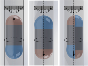
The theoretical derivation in this section assumes azimuthal symmetry in the bubble profile (figure 1a–c). An axisymmetric bubble, for example in figure 1(a), can be divided into three regions: a leading spherical cap (region  $I$, also known as the ‘nose’), which smoothly connects to a uniform film region with thickness
  $b$ (region
  $II$), and a trailing spherical cap (region
  $III$, also known as the ‘tail’), which connects to region
  $II$ with undulations. For a bubble in a vertically oriented capillary under an external flow, two possible axisymmetric bubble profiles can be obtained, including the ‘nose-up’ (figure 1b) and the ‘nose-down’ (figure 1c) configurations. In this section, theoretical derivations will be provided to solve for the uniform film thickness in these two cases.

Figure 1. Schematics of bubble profiles. Bubbles are confined in a vertically oriented cylindrical capillary under an external flow, which is characterized by the cross-sectional averaged fluid velocity  $U_l$, whose magnitude is shaded in dark grey. (a) Different regions in an axisymmetric bubble profile. The axisymmetric bubble profile is characterized by three distinct regions:
  $I$ (shaded red), the bubble ‘nose’;
  $II$, uniform film region; and
  $III$ (shaded blue), the bubble ‘tail’. As shown by the arrows in the insets, when moving away from the uniform film region
  $II$, the film thickness connecting to the nose varies monotonically, while the film connecting to the bubble tail exhibits undulations. (b) Axisymmetric bubble profile with the nose pointing upwards and the uniform film thickness
  $h(x) = b$ in region
  $II$. The inset shows a parabolic velocity profile
  $u(y)$ in region
  $II$ in the laboratory frame. (c) Axisymmetric bubble profile with the nose pointing downwards. Note that panels (b) and (c) are illustrated at the same magnitude of downward flow speed
  $U_l$, suggesting the non-unique film profiles under the same flow conditions. (d) The symmetry-breaking bubble profile, which shows the cross-section with the maximum (left) and minimum (right) film thicknesses. While the thick film adopts a profile with the nose (red) pointing upwards and the tail (blue) pointing downwards, the profile of the thin film has the opposite arrangement. The bubble centreline offsets from the tube centreline towards the thin film. The symmetry breaking will be discussed in § 4.2.
As mentioned previously, the classic Bretherton problem in a horizontal capillary can be considered as the special case with  ${Bo} = 0$. In the absence of buoyancy effects, the tube orientation does not alter the dynamics, and the uniform film thickness is solely determined by the magnitude of the external flow. The film thickness vanishes as
  ${Ca}_l\to 0$, with the direction of the bubble motion and the bubble nose pointing in the same direction as the external flow.
In the case where  ${Bo}$ is not negligible, the dynamics of the bubble are governed by the combination of viscous and capillary effects, buoyancy and the external flow. Since a bubble can spontaneously rise through a stagnant fluid in a vertically oriented capillary when
  ${Bo} > {Bo}_{cr}$, it is intuitive that this bubble might sustain a small magnitude of the downward flow and continue to rise. As will be shown later in this section, the directional alignment between the two driving forces will significantly affect the axisymmetric bubble profile, which can be categorized naturally in one of two cases: a bubble with the ‘nose’ pointing upwards or downwards. In this problem, the Bond number
  ${Bo}= \rho g R^2/\gamma$ and the capillary number of the external flow
  ${Ca}_l = \mu U_l/\gamma$ are both given. Based on the input, we seek to uncover the dynamics of the bubble at steady state, especially the uniform film thickness
  $b/R$ as well as the non-dimensional speed, or the capillary number of the bubble,
  ${Ca}_b = \mu U_b/\gamma$. Hereafter, negative values of the liquid or bubble capillary number are associated with downward liquid or bubble flow.
2.1. ‘Nose-up’ branch: bubble profile with nose pointing upwards
We begin by summarizing the results from Magnini et al. (Reference Magnini, Khodaparast, Matar, Stone and Thome2019), who investigated the dynamics of a confined bubble translating at steady state under an external upward flow. In fact, with a small variation, as we will describe in the following context, it can be extended to describe a more general case: the dynamics of a bubble with its ‘nose’ pointing upwards (figure 1b).
As indicated in figure 1(b), the coordinates are represented by  $(x, y)$, with
  $x$ pointing vertically upwards and
  $y = R- r$ pointing radially inwards from the tube inner wall. With the assumption that the film thickness is much smaller than the tube radius,
  $b/R\ll 1$, (
 $x,y$) can effectively be treated as local Cartesian coordinates, and the lubrication approximation can be applied to simplify the Navier–Stokes equations as
 \begin{gather} \text{continuity}\quad u_x +v_y= 0, \end{gather}
 \begin{gather}x\text{-direction}\quad u_{yy} = \frac{1}{\mu} \left(p_x + \rho g \right), \end{gather}
 \begin{gather}y\text{-direction}\quad p_y = 0, \end{gather}
where subscripts denote derivatives, the velocities in  $(x, y)$ are represented by
  $(u, v)$ and
  $p$ denotes the fluid pressure.
In a reference frame moving with the bubble at the steady-state speed  $U_b$, the velocity profile within the thin film can be obtained by integrating equation (2.1b) with the boundary conditions
 \begin{equation} u\big\vert_{y = 0} = -U_b \quad \text{and} \quad u_y \big\vert_{y = h(x)} = 0, \end{equation}
which results in
 \begin{equation} u(y) = \frac{1}{2\mu} (p_x + \rho g ) (y^2 - 2hy ) - U_b. \end{equation}
Note that, due to the gravitational effects, fluid in the thin film is always draining vertically downwards with a parabolic profile. Specifically, the velocity profile within the uniform film region  $u_b(y) = \rho g (y^2 - 2by)/(2\mu ) - U_b$ can then be obtained by demanding
  $h(x) = b$ and
  $p_x = 0$ from (2.3). An expression for
  $\kappa _x$, the gradient of curvature along the
  $x$-direction, can thus be obtained by matching the fluxes from integrating the two velocity profiles, and, consistent with the relative magnitude of terms in the lubrication approximation, expressing the gradient of capillary pressure as
  $p_x = -\gamma \kappa _x$:
 \begin{equation} \kappa_x = \frac{3\mu U_b}{\gamma}\frac{(h-b)}{h^3} + \frac{\rho g}{\gamma}\frac{(h^3 - b^3)}{h^3}. \end{equation}
The two terms in (2.4) indicate the contributions from the capillary and buoyancy effects, respectively. This expression for  $\kappa _x$, obtained from the lubrication equations, can be equated to its geometrical counterpart,
  $\kappa _x = (\boldsymbol {\nabla }\boldsymbol {\cdot } \boldsymbol {n})_x$, where
  $\boldsymbol {n}$ denotes the normal vector of the bubble surface pointing inwards to the gas phase (figure 1b), leading to
 \begin{equation} \frac{3\mu U_b}{\gamma}\frac{(h-b)}{h^3} + \frac{\rho g}{\gamma}\frac{(h^3 - b^3)}{h^3} = \left[ \frac{1}{(h_x^2 + 1)^{1/2}}\frac{1}{R-h} + \frac{h_{xx}}{(h_x^2 + 1)^{3/2}} \right]_x. \end{equation}
 As noticed previously (Magnini et al. Reference Magnini, Khodaparast, Matar, Stone and Thome2019), the full expression for the curvature of the film profile is necessary in order for (2.4) to describe the liquid flow in both the thin film and bubble cap regions. One can further proceed with non-dimensionalization by defining  $X = x/\ell$,
  $H = h/b$ and
  $K = \kappa \ell ^2/b$, with
  $\ell$ denoting the characteristic length scale in the
  $x$-direction, which will be determined below. Different from Magnini et al. (Reference Magnini, Khodaparast, Matar, Stone and Thome2019), non-dimensionalizing (2.5) shows that there are two choices for the characteristic scale
  $\ell$, which lead to two different expressions for
  $\epsilon \equiv b/\ell$:
 \begin{equation} \epsilon_1 = {Ca}_b^{1/3} \quad \text{or} \quad \epsilon_2 = ( \alpha^2 {Bo} )^{1/3}, \end{equation}
where  $\alpha = b/R$. Note that
  $\epsilon _1$ and
  $\epsilon _2$ are consistent with the characteristic scales for the classic Bretherton problems in horizontal (
 ${Bo} = 0$) and vertical orientations (
 ${Ca}_l = 0$), respectively. Furthermore, the ratio between these two choices,
  ${\lambda \equiv (\epsilon _2/\epsilon _1)^3 = \alpha ^2 {Bo}/{Ca}_b}$, quantifies the relative significance of the buoyancy and capillary effects within the thin film region. While the right-hand side (RHS) of the rescaled equation (2.5) shows
 \begin{equation} \text{RHS} = \frac{H_{XXX}}{f^3} - \frac{3 \epsilon^2 H_X H_{XX}^2}{f^5} - \frac{\alpha}{1-\alpha H}\frac{H_X H_{XX}}{f^3} + \left( \frac{\alpha}{1-\alpha H}\right)^2\frac{H_X}{\epsilon^2 f}, \end{equation}
with  $f = (\epsilon ^2H_X^2 + 1)^{1/2}$, different choices of
  $\epsilon$ result in a slightly different left-hand side (LHS) of the rescaled equation (2.5):
 \begin{gather} \epsilon = \epsilon_1, \quad \text{LHS} = 3 \frac{(H-1)}{H^3} + \lambda \frac{(H^3-1)}{H^3}, \end{gather}
 \begin{gather}\epsilon = \epsilon_2, \quad \text{LHS} = \frac{3}{\lambda} \frac{(H-1)}{H^3} + \frac{(H^3-1)}{H^3}. \end{gather}
 When the system is provided with an upward external flow, as in Magnini et al. (Reference Magnini, Khodaparast, Matar, Stone and Thome2019), both length-scale choices are well defined and thus perform equivalently. When solving for the film profile with a downward flow, however, choosing  $\epsilon _1$ becomes problematic, as
  ${Ca}_b\to 0$, which leads to an artificial singularity in the term associated with
  $\lambda$ in (2.8a).
As a result, in order to extend the film profile solution with an upward nose towards the downward flow regime, while avoiding the artificial singularity, the characteristic length scale is chosen interactively during the numerical shooting process (see § 2.3 for more detail):  $\epsilon = \epsilon _1$ is chosen when
  $\lambda < 1$, where capillary effects outweigh buoyancy in the thin film and (2.7) and (2.8a) are solved; otherwise, when
  $\lambda \geqslant 1$,
  $\epsilon = \epsilon _2$ is chosen and (2.7) and (2.8b) are solved.
Note that, in the simulations and physical experiments, the strength of the external flow,  ${Ca}_l$, is directly controlled rather than the bubble speed,
  ${Ca}_b$, which enters
  $\lambda = \alpha ^2{Bo}/{Ca}_b$. Therefore, an additional relationship is needed to link the two capillary numbers, which can be obtained by balancing the flux from the external Poiseuille flow in the far field and the cross-sectional flux in the uniform film region. Integrating the velocity profiles in cylindrical coordinates, we have
 \begin{equation} {Ca}_b = \frac{{Ca}_l}{(1-\alpha)^2} + {Bo} \left[-\frac{1}{2} + \frac{3 (1-\alpha)^2 }{8} + \frac{1}{8(1-\alpha)^2} -\frac{1}{2} (1-\alpha )^2 \log(1-\alpha) \right]. \end{equation}
 With any two of  ${Bo}$,
  ${Ca}_l$,
  ${Ca}_b$ and
  $\alpha = b/R$ given, one can solve (2.7)–(2.9) for the other quantities with numerical shooting (see § 2.3). One of the questions of interest is the critical strength of the external downward flow needed,
  ${Ca}_{l, cr}$, in order to stabilize the bubble, i.e.
  ${Ca}_b = 0$. In this scenario, the critical magnitude of external flow
  ${Ca}_{l, cr}$ and the corresponding film thickness
  $\alpha = b/R$ can be solved based on the two inputs – the Bond number
  ${Bo}$ and
  ${Ca}_b = 0$.
Typical results from a numerical solution are shown in figure 2, where the critical downward flow  ${Ca}_{l, cr}$ as a function of
  ${Bo}$ is shown as the black solid curve in figure 2(a). For a fixed
  ${Bo}$, the bubble rises if the provided external flow is above the curve with
  ${Ca}_{l}>{Ca}_{l, cr}$, and vice versa. This solution is consistent with the results for a vertically oriented capillary in Bretherton (Reference Bretherton1961), as
  ${Ca}_{l, cr}$ = 0 remains true for all
  ${Bo} <{Bo}_{cr}$, and non-zero downward flow is needed to maintain the bubble stationary in the laboratory frame otherwise. The magnitude of
  ${Ca}_{l, cr}$ remains small for
  ${Bo} \approx 1$, and rapidly increases as gravitational effects become more dominant.

Figure 2. Critical condition for a bubble being stabilized in the laboratory frame ( $Ca_b = 0$) under an external downward flow. (a) The critical strength of the external flow
  ${Ca}_{l,cr}$ as a function of
  ${Bo}$. Consistent with results in the literature, external downward flow is needed to keep the bubble stationary in the laboratory only for
  ${Bo} > {Bo}_{cr}$, and, as
  ${Bo}$ increases, a stronger downward flow is required. (b) The uniform film thickness
  $b/R$ when the critical external flow condition
  ${Ca}_{l,cr}$ is applied, where
  $\alpha = b/R$ monotonically increases with
  ${Ca}_{l,cr}$. In the limit of
  $\alpha \to 0$, expanding (2.9) shows that
  $\alpha \sim (-{Ca}_{l,cr}/{Bo})^{1/3}$, and the asymptotic scaling is shown as the red dashed curve.
The corresponding critical film thickness is shown in figure 2(b), where the inset is plotted in log–log scales. Note that, in the limit of  $\alpha \to 0$, (2.9) can be expanded. Since both the external flow and buoyancy are significant, taking the leading order of each term and demanding
  ${Ca}_b = 0$ (a stationary bubble) leads to
 \begin{equation} \alpha =\left(-\frac{3}{2}\frac{{Ca}_{l,cr}}{{Bo}}\right)^{1/3}. \end{equation}
This asymptotic approximation is shown in figure 2(b) as the red dashed curve, which is in excellent agreement with the numerical shooting solutions for  $\alpha = b/R < 0.1$. Furthermore, the rapid increase of
  ${Ca}_{l, cr}$ with
  ${Bo}$ can thus be qualitatively explained, since the critical film thickness increases with
  ${Bo}$, and the scaling shows
  $|{Ca}_{l, cr}| \sim \alpha ^3{Bo}$.
2.2. ‘Nose-down’ branch: bubble with nose pointing downwards
Equations (2.7)–(2.9) fully describe the dynamics of the bubble under an upward external flow ( ${Ca}_{l} \geq 0$). For
  ${Bo} > {Bo}_{cr}$, the solution can be further extended towards the downward flow regime (
 ${Ca}_{l} < 0$), with the bubble nose pointing upwards and
  ${Ca}_b \to {Ca}_l^+$. However, this solution is only valid for a limited range of
  ${Ca}_{l} < 0$, beyond which solutions of (2.7)–(2.9) fail to converge within the set tolerance, and thus the branch terminates. In a physical system, the bubble responds to the stronger downward flow by changing its morphology, so that the ‘nose’ points downwards as indicated in figure 1(c), following the flow direction. Both experiments and simulations introduced in the next sections will confirm this response.
The bubble profile in a downward-nose system is similar to the upward-nose case, and therefore, when it comes to solving for the film profile, the new film equations can be obtained by modifying (2.7)–(2.9) simply by redefining the vertical coordinate as  $\tilde {x} = -x$ (figure 1c). With this convention, the positive directions of
  ${Ca}_l$ and
  ${Ca}_b$ within the model are redefined, while the scalar variables (e.g.
  $\alpha$ and
  $H$) remain unchanged. Furthermore, since the gravitational direction remains vertically downwards regardless of coordinates, in the new coordinate system, the terms associated with
  ${Bo}$ must change sign as well. As a result, the film equations become
 \begin{gather} 3 \frac{(H-1)}{H^3} - \lambda \frac{(H^3-1)}{H^3} = \frac{H_{XXX}}{f^3} - \frac{3 \epsilon^2 H_X H_{XX}^2}{f^5} - \frac{\alpha}{1-\alpha H}\frac{H_X H_{XX}}{f^3} + \left( \frac{\alpha}{1-\alpha H}\right)^2\frac{H_X}{\epsilon^2 f}, \end{gather}
 \begin{gather}{Ca}_b = \frac{{Ca}_l}{(1-\alpha)^2} - {Bo} \left[-\frac{1}{2} + \frac{3 (1-\alpha)^2 }{8} + \frac{1}{8(1-\alpha)^2} -\frac{1}{2} (1-\alpha )^2 \log(1-\alpha) \right], \end{gather}
where, compared to (2.7)–(2.9), the net effects are sign changes in the terms related to gravity only. In other words, by changing the nose direction from upwards to downwards, the bubble only senses a sign change in the buoyancy force: instead of assisting the bubble to rise, buoyancy effects are now acting as resistance to the bubble motion, which is now mainly driven by the downward external flow.
When the bubble dynamics falls on this solution branch, the bubble always sinks and the film thickness  $\alpha$ converges to the origin as
  ${Ca}_l \to 0^-$ (as we will confirm in § 4). Thus,
  $\epsilon = \epsilon _1$ is chosen when non-dimensionalizing the equations, resulting in the form of (2.11a) similar to (2.8a).
2.3. Numerical integration
With  ${Ca}_l$ and
  ${Bo}$ given, (2.7)–(2.9) or (2.11) can be solved for
  ${Ca}_b$, the uniform film thickness
  $\alpha$ and the film profile
  $H(X)$, with the boundary conditions
 \begin{equation} H(0) = 1, \quad H_X(0) = 0 \quad \text{and} \quad H_{XX}(0) = 0, \end{equation}
and  $H(X_{nose}) = 1/\alpha$ is demanded as the additional constraint, with
  $X = 0$ indicating the uniform film region and
  $X_{nose}$ the location of the bubble nose, which is yet to be determined by the numerical integration scheme. Although the full curvature of the film is used in (2.7)–(2.9) or (2.11), the underlying solution method is effectively the same as the asymptotic expansion as seen in Bretherton (Reference Bretherton1961), which includes the process of solving the film equation for the bubble ‘nose’ and matching to the static spherical cap. The coupled equations are solved by first imposing an initial guess on
  $\alpha$. With
  ${Ca}_l$ and
  ${Bo}$ given, (2.9) or (2.11b) outputs the capillary number of the bubble
  ${Ca}_b$, which serves as an input for (2.7) and (2.8) or (2.11a). The ordinary differential equation for
  $H(X)$ is solved by numerical integration with the MATLAB program
  $ode45$ from the uniform film region towards the front spherical cap in the positive
  $X$-direction. Numerical integration ceases when
  $H_X \to \infty$, where the termination location denotes
  $X_{nose}$ and the value
  $H(X_{nose})$ is compared with the constraint
  $H(X_{nose}) = 1/\alpha$. The initial guess of
  $\alpha$ is then iteratively updated until this additional constraint is met, meaning that the bubble nose is symmetric about the tube centreline.
3. Experimental and numerical simulation methods
3.1. Experimental set-up
Experiments are performed in a refractive-index-matching set-up similar to those described in Yu et al. (Reference Yu, Zhu, Shim, Eggers and Stone2018) and Magnini et al. (Reference Magnini, Khodaparast, Matar, Stone and Thome2019), with pure glycerol filling the capillary tube as the continuous phase. The density, viscosity and surface tension of the pure glycerol are measured as  $\rho = (1.29 \pm 0.001) \times 10^3\ \textrm {kg}\,\textrm {m}^{-3}$,
  $\mu = 1.00 \pm 0.04\ \textrm {Pa}\,\textrm {s}$ (Anton Parr, Physica MCG 301) and
  $\gamma = 65.4 \pm 1.0\ \textrm {mN}\,\textrm {m}^{-1}$ (pendant drop), respectively. Glass capillaries with three different inner diameters (
 $ID = 4.45, 4.85, 5.65 \pm 0.05\ \textrm {mm}$) are used, yielding the Bond numbers of
  ${Bo} = 0.97, 1.16, 1.56$, respectively. Each glass capillary is placed within a cuboid glass box, which is also filled with pure glycerol in order to avoid imaging distortions. The top end of the glass capillary is connected to a liquid reservoir by a Teflon hose, and the bottom end is submerged in a bath of pure glycerol. The experimental flow rate is adjusted by controlling the reservoir pressure using the Elveflow
 $^{\circledR }$ OB1 MK3 pressure and vacuum controller, and calibration between the flow rate and controller pressure is performed for all capillary tubes used. The imaging apparatus is composed of a Nikon D5100 DSLR camera and a Mitutoyo infinity-corrected objective, mounted on an in-house-made tube microscope. The imaging apparatus is aligned horizontally with a collimated LED source, which is located half-way between the two ends of the capillary tube.
In each set of experiments with the same  ${Bo}$, the capillary tube is partially filled with pure glycerol, leaving a section of an air column in the bottom end of the capillary. The set-up is then carefully calibrated to be vertical. A single bubble is formed by applying vacuum to the system, providing an upward flow and assisting the formation of the thin liquid film. For experiments corresponding to
  ${Ca}_b > 0$, experiments start by directly setting the pressure/vacuum to a target value; for experiments with
  ${Ca}_b < 0$, on the other hand, the target pressure value is set after the bubble rises to the top end of the capillary. As the bubble reaches the region of interest of the imaging apparatus, the dynamics of the bubble are recorded in the bright-field mode at 30 frames per second. After each experiment, the bubble velocity and the film profile are analysed from the image sequence, and the capillary number of the external flow
  ${Ca}_l$ is calculated based on the calibration between flow rate and pressure control.
3.2. Numerical simulation set-up
Direct numerical simulations of the flow of elongated bubbles in vertical capillaries are performed utilizing the volume-of-fluid (VOF) method (Hirt & Nichols Reference Hirt and Nichols1981) implemented in OpenFOAM. The unsteady mass and momentum equations for an incompressible flow and Newtonian fluid are solved, together with a transport equation for a passive scalar that identifies the gas and liquid phases across the domain. In this formulation, the surface tension force is implemented as a body force according to the continuum surface force method (Brackbill, Kothe & Zemach Reference Brackbill, Kothe and Zemach1992). Both two-dimensional axisymmetric and full three-dimensional simulations are conducted, with the latter enabling us to investigate conditions that may lead to symmetry breaking. The simulation set-up is similar to that adopted in previous works (Magnini et al. Reference Magnini, Ferrari, Thome and Stone2017, Reference Magnini, Khodaparast, Matar, Stone and Thome2019). An elongated bubble, with the shape of a cylinder with spherical ends, is initialized at one end of the flow domain. Bubble lengths of approximately  $6D$ are sufficient to achieve a uniform film region between front and rear menisci, under the conditions of interest. At the inlet boundary, a fully developed laminar profile is set for the incoming liquid, while no slip is set at the pipe wall. At the channel outlet, pressure is given a constant value, together with a zero-gradient condition for the velocity. The liquid-to-gas density and viscosity ratios are set to 1000 and 100, respectively. Each simulation is run forwards in time until the bubble translates with a constant speed.
Numerical simulations are performed for the three values of the Bond number tested experimentally and a wide range of  ${Ca}_l$, for both upward and downward liquid flow. For each value of
  ${Bo}$ and each flow direction, a first simulation is run with the largest
  $|{Ca}_l|$ desired, until steady state. From this steady solution,
  $|{Ca}_l|$ is reduced and a new simulation is run until a new steady bubble profile and speed are achieved. The procedure continues by stepping towards smaller values of
  $|{Ca}_l|$ to span the entire range of conditions of interest, each time until steady state.
4. Results and discussion
The comparison between theory, experiments and numerical simulations is shown in figure 3 for  ${Bo} = 0.97$. The film thickness
  $b/R$ as a function of
  ${Ca}_l$ is plotted in figure 3(a), where results from theory (solid curves), experiments (circles) and numerical simulations (squares) show good agreement. The theoretical results from numerical shooting predict two distinct solution branches of the film thickness: the ‘nose-down’ branch is obtained by solving (2.11), where the bubble nose is pointing downwards; and the ‘nose-up’ branch is obtained from solving (2.7)–(2.9), with the bubble nose pointing upwards. Note that, since the Bond number
  ${Bo} = 0.97 > {Bo}_{cr}$, the ‘nose-up’ branch intersects with the
  $y$-axis (stagnant fluid) at a non-zero value of the film thickness. As
  $Ca_l$ decreases towards the downward flow regime, the ‘nose-up’ branch extends towards
  $b/R\to 0$, but only exists in a very narrow range of downward flow before it terminates; this aspect will be more apparent at the larger Bond numbers presented in the next section.

Figure 3. Comparison between lubrication theory, experiments and simulations at  ${Bo} = 0.97$. (a) Plot of film thickness
  $b/R$ versus
  ${Ca}_l$. Solid curves represent the theoretical results from numerical shooting, with the ‘nose-down’ branch obtained from solving (2.11), and the ‘nose-up’ branch from solving (2.7)–(2.9). Results from experiments (circles) and direct numerical simulations (squares) both agree with the theoretical prediction and verify the existence of two distinct branches. Specifically, the red and blue markers represent the cases shown in panels (b,c) and (d,e), respectively. (b,c) Bubble with nose pointing downwards,
  $Ca_l=-0.8 \times 10^{-3}$, where undulations appear on the top end of the bubble. Bubble profiles are compared in (c), where the theoretical profile (red dash-dotted curve) is plotted on the left, and the profile from numerical simulation (green dashed curve) is plotted on the right. (d,e) Bubble with nose pointing upwards,
  $Ca_l=1.1 \times 10^{-3}$, with undulations appearing on the bottom end. Results are compared in (e) with the theoretical profile (red dash-dotted curve) on the left, and the simulation profile (green dashed curve) on the right.
As displayed in figure 3, under the same magnitude of the external flow, the film thickness on the ‘nose-up’ branch is consistently larger than that on the ‘nose-down’ branch. As an example, typical experimental images are shown for a sinking bubble (figure 3(b,c), corresponding to the red markers in figure 3a) and a rising bubble (figure 3(d,e), corresponding to the blue markers in figure 3a). While the sinking bubble shown in the figure has its nose pointing downwards and undulations appear near the top end, the rising bubble has its nose pointing upwards and undulations appear near the bottom end. For the two cases undergoing an external flow of similar magnitude, the sinking bubble (figure 3c) shows a film thickness of  $b/R = 7.6\times 10^{-3}$, which is much smaller than that of a rising bubble (figure 3e), whose film thickness is
  $b/R = 5.0\times 10^{-2}$. Furthermore, the film profiles near the bubble nose are also compared. As shown in figure 3(c,e), the theoretical film profiles are plotted as red dash-dotted curves, overlaying on the left half of the experimental images, and the profiles from simulations are plotted as green dashed lines on the right. In both cases, good agreement is obtained among the theoretical, experimental and numerical results.
4.1. Effects of Bo and the non-unique, history-dependent film profiles
Results for different Bond numbers  ${Bo} = \{0.97, 1.16, 1.56\}$ are displayed in figure 4. Note that only the results of experiments and simulations terminating with an axisymmetric bubble profile are included in the figure, whereas symmetry-breaking configurations will be discussed in § 4.2. As the Bond number increases in figure 4(a,c,e), the two film thickness branches deviate more from the classic theory (equation (1.1), shown as grey dashed curves), and the difference between the two branches also increases. As the film thickness on the ‘nose-up’ branch increases along with
  ${Bo}$, the branch intersects with the
  $y$-axis at a larger value of
  $b/R$. The ‘nose-down’ branch, however, has the film thinning as
  ${Bo}$ increases, which is consistent with physical intuition. When the bubble translates with an upward nose, buoyancy serves as the main driving force of the motion, and the external flow acts as a side factor, assisting or hindering the bubble motion depending on the sign of
  ${Ca}_l$. As a result, the bubble has an increased tendency to rise as
  ${Bo}$ increases, and thus forms a thicker film. On the other hand, the external flow serves as the main driving force when the bubble sinks with a downward nose, while gravity remains a resistance to the bubble motion, thus resulting in the thinning of the film thickness at higher
  ${Bo}$. Meanwhile, comparing
  ${Ca}_b$ and
  ${Ca}_l$ at various
  ${Bo}$ (figure 4b,d,f) shows that the bubbles with downward noses always sink with
  ${Ca}_b<{Ca}_l$. On the other hand, the bubbles on the ‘nose-up’ branch follow
  ${Ca}_b > {Ca}_l$ over a wide range of
  ${Ca}_l$, except for a very narrow region near the branch termination (see insets of figure 4b,d,f).

Figure 4. Overlapping solution branches and the non-unique film profiles for  ${Bo} > {Bo}_{cr}$. Results at (a,b)
  $Bo = 0.97$, (c,d)
  $Bo = 1.16$ and (e,f)
  $Bo = 1.56$ are shown, comparing theory (solid curves), experiments (circles) and numerical simulations (squares). Results corresponding to the ‘nose-down’ branch (thin film) and ‘nose-up’ branch (thick film) are coloured in red and blue, respectively. (a,c,e) Relationships between the film thickness
  $b/R$ and external flow
  ${Ca}_l$. As
  ${Bo}$ increases, the two solution branches deviate more from the classic
  ${Bo}=0$ theory (grey dashed curves) and overlap over a larger region of downward flow. (b,d,f) Comparisons between
  ${Ca}_b$ and
  ${Ca}_l$, with the black dashed line indicating the reference
  ${Ca}_b = {Ca}_l$. While
  ${Ca}_b < {Ca}_l$ is observed on the ‘nose-down’ branch, the ‘nose-up’ branch mainly follows
  ${Ca}_b > {Ca}_l$, except at a very narrow region close to where the branch terminates. The insets show a close-up view of the overlapping regions of the branches, where the history-dependent bubble dynamics are observed both theoretically and numerically.
Furthermore, we observe from both the film thickness and bubble capillary number plots that the ‘nose-up’ branch extends towards the downward flow regime, with the extended domain enlarging for increasing values of the Bond number, whereas the ‘nose-down’ branch always converges to the origin as  ${Ca}_l\to 0^-$. These results suggest that there is a range of downward flows where the two branches overlap for the same
  ${Bo}$ and
  ${Ca}_l$, and hence the bubble film profile undergoes ‘hysteresis’-like history-dependent dynamics in the overlapping domain of the two branches.
As an example, the inset of figure 4(f) shows the simulation results of two different film profiles obtained under the same conditions of  ${Bo}= 1.56$ and
  ${Ca}_l = -2\times 10^{-3}$. When the bubble profile is obtained starting from a steady-state configuration at
  ${Ca}_l=0$, the solution stays on the ‘nose-up’ branch (blue squares), which corresponds to a bubble sinking at
  ${Ca}_b = -7.5\times 10^{-4}$ (
 ${Ca}_b>{Ca}_l$) with a thick film of thickness
  $b/R = 1.2\times 10^{-1}$ and its nose pointing upwards. However, a distinct solution is obtained when reaching
  ${Ca}_l = -2\times 10^{-3}$ from a steady-state profile at a smaller (more negative)
  ${Ca}_l$, which belongs to the ‘nose-down’ branch. The solution stays on the ‘nose-down’ branch (red squares), and the bubble sinks at
  ${Ca}_b = -2.1\times 10^{-3}$ (
 ${Ca}_b<{Ca}_l$) with a much thinner film of thickness
  $b/R = 1.5\times 10^{-2}$ and its nose pointing downwards.
To summarize the evolution of the two branches at different  ${Bo}$, a phase diagram for the axisymmetric bubble profile is generated from the theoretical results and shown in figure 5. The classic theoretical results with
  ${Bo} = 0$ are plotted as black solid curves, which are symmetric about the
  $y$-axis. When an external upward flow is applied, the bubble profile is uniquely determined by the combination of
  ${Bo}$ and
  ${Ca}_l>0$, and, for the same
  ${Ca}_l$, the film thickness increases with
  ${Bo}$. Note that, for
  ${Bo}<{Bo}_{cr}$, the film thickness converges to the origin as
  ${Ca}_l\to 0^+$, which is consistent with the original work of Bretherton (Reference Bretherton1961). For
  ${Bo}>{Bo}_{cr}$, on the other hand, the ‘nose-up’ branch extends into a limited range of downward flow speeds. The bubble continues to rise until the ‘nose-up’ branch intersects with the black dash-dotted curve denoting
  ${Ca}_b = 0$, and this axisymmetric solution branch eventually terminates at the black dashed curve, beyond which the numerical shooting method fails to converge within the set tolerance when (2.7)–(2.9) are solved.

Figure 5. Phase diagram obtained from numerically integrating equations (2.7)–(2.9) and (2.11), showing the film thickness  $b/R$ versus
  ${Ca}_l$ and the evolution of the branches with varying
  ${Bo}$. The two branches corresponding to the same
  ${Bo}$ are labelled with the same colour code. Also shown in each regime are schematics of the typical bubble profile. While the ‘nose-up’ branches with
  ${Bo} < {Bo}_{cr}$ converge to the origin, the ‘nose-up’ branches with
  ${Bo} > {Bo}_{cr}$ extend in the downward flow regime. The black dotted curve and black dashed curve represent the critical conditions where
  ${Ca}_b =0$ and
  ${Ca}_b ={Ca}_l$, respectively. The black dash-dotted curve shows the conditions where the ‘nose-up’ branches terminate in the numerical shooting schemes. Note that the ‘nose-up’ branches are shown as dashed between
  ${Ca}_b ={Ca}_l$ and the branch termination conditions, since no axisymmetric bubble profiles are observed in experiments or three-dimensional numerical simulations within this range, as will be explained in § 4.2.
If  ${Ca}_l$ is further decreased beyond the region where the ‘nose-up’ branch terminates, axisymmetric solutions can only be found on the ‘nose-down’ branch with the bubble nose pointing downwards, as shown in figure 5, with the colour code being the same as for the corresponding ‘nose-up’ branch. With the external flow serving as the main driving force, for the same value of
  ${Ca}_l$, the bubble film thickness on the ‘nose-down’ branch decreases with the increasing resistance from
  ${Bo}$. Since all solutions on the ‘nose-down’ branches converge to the origin as
  ${Ca}_l\to 0^-$, the solution branches overlap in the region where the ‘nose-up’ branch extends in the downward flow regime, and the overlap region enlarges with increasing
  ${Bo}$, indicating the non-unique and history-dependent film thickness solutions.
4.2. Symmetry breaking
Numerical shooting results indicate that axisymmetric bubble profiles are not available in the downward flow region between the black solid curve (the ‘nose-down’ branch with  ${Bo} = 0$) and the black dash-dotted curve (where the ‘nose-up’ branches terminate), where both experiments and three-dimensional simulations exhibit symmetry-breaking profiles, as will be shown below; see sketch in figure 1(d). Note that axisymmetry-breaking bubble profiles are known in the literature for pipe flows with
  ${Bo} \geq {O}(10)$, where the bubble breaks symmetry in external flows with large inertial effects (
 ${Re} \gtrsim {O}(100)$), often with fragmented bottoms (see e.g. Griffith & Wallis Reference Griffith and Wallis1961; Martin Reference Martin1976; Lu & Prosperetti Reference Lu and Prosperetti2006; Fabre & Figueroa-Espinoza Reference Fabre and Figueroa-Espinoza2014; Fershtman et al. Reference Fershtman, Babin, Barnea and Shemer2017). In contrast, the symmetry-breaking profiles obtained in the current work, as shown in figure 6(a,b), exist in an inertialess regime with
  ${Bo} \leq {O}(1)$ and
  $|{Ca}_l|\leq {O}(10^{-2})$. The bubble profile thus preserves some features associated with the classic lubricating film in an axisymmetric bubble.

Figure 6. Symmetry-breaking bubble profiles in experiments and simulations. (a) Symmetry-breaking profiles obtained from experiments, with  ${Bo} = 0.97$ and
  ${Ca}_l = -1.7\times 10^{-3}$. Note that the ‘nose’ (shaded red) and ‘tail’ (shaded blue) of the bubble are the sections connecting to the uniform film region without and with undulations, respectively. A thick film is shown on the left-hand side with the bubble nose pointing upwards, and a thin film is shown on the right-hand side with the bubble nose pointing downwards. From the tube centreline (black dash-dotted line), the bubble centreline (red dashed line) is shifted towards the side of the thin film. (b–d) Symmetry-breaking profiles obtained from a three-dimensional numerical simulation at
  ${Bo} = 1.56$ and
  ${Ca}_l = -4.0\times 10^{-3}$, started from a steady-state configuration (
 ${Ca}_l = -3.0\times 10^{-3}$) belonging to the ‘nose-up’ branch. (b) The symmetry-breaking profiles are consistent with the image obtained from experiments, with the colour code representing the downward fluid velocity normalized by
  $U_l$. (c) The circumferential bubble profile approximately half-way between the bubble top and bottom (as indicated by the dashed line in panel b), where the cross-section of the bubble is no longer circular. (d) The bubble profile in the
  $y'$–
$y'$– $z'$ plane. The black solid circle represents the tube inner wall, and the black dashed circle and the red curve represent the initial axisymmetric bubble profile and the asymmetric bubble surface, respectively.
Both experiments and three-dimensional simulations yield symmetry-breaking profiles when the bubble attempts to transit between steady states near the ends of the two branches, while the bubble is sinking and adapting to a new steady-state profile by thinning the film. While the symmetry-breaking profiles are supported by both experiments and three-dimensional simulations, we noticed that symmetry breaking occurs before the theoretically predicted branch termination conditions are met, and no ‘nose-up’ axisymmetric profiles are observed when  ${Ca}_b < {Ca}_l$. Though the detailed mechanism accounting for the symmetry-breaking process is out of the scope of the current work, the discrepancies in the critical conditions might be explained in several different ways. First, the symmetry-breaking process is triggered near the upper spherical caps (the bubble ‘nose’ if at a ‘nose-up’ profile, or the ‘tail’ if ‘nose down’). However, the theoretical predictions are based on an axisymmetric profile assumption, with the derivation mainly focusing on the uniform film thickness region. Furthermore, we observed that the bubble profile becomes more sensitive to system perturbations when the conditions are closer to the branch termination. Therefore, while the theoretical predictions might provide an ‘ideal boundary’, the system perturbations in experiments or finite resolutions in simulations can account for the early trigger to the symmetry-breaking process.
Here, we report the evidence of such profiles and provide qualitative descriptions of the symmetry-breaking process.
4.2.1. Asymmetric bubble profiles
Two symmetry-breaking bubble profiles are shown in figure 6(a,b), with figure 6(a) obtained from an experiment, and figure 6(b) from a three-dimensional direct numerical simulation (see § 3 for the experimental and numerical simulation set-ups). While the experimental figure is captured in the vertical plane, near where the maximum and minimum film thicknesses exist, the simulation figure is plotted at the vertical plane where  $y'=0$, with
  $x', y',z'$ denoting the coordinates in the three-dimensional numerical simulation. Unlike the asymmetric profiles reported in the literature (e.g. Fabre & Figueroa-Espinoza Reference Fabre and Figueroa-Espinoza2014; Fershtman et al. Reference Fershtman, Babin, Barnea and Shemer2017), both the top and bottom caps of the bubble surface are present, and, because of this, distinct features are observed about the film profile. Note that the bubble ‘nose’ and ‘tail’ are the sections connected to the uniform film region without and with undulations, respectively. As indicated in figure 6(a,b), on the portion of the bubble surface associated with a thick film, the bubble has its nose pointing upwards and undulations appear at the bottom. On the portion with a thin film, on the other hand, the bubble has its nose pointing downwards and the undulations appear on the top. Connecting the top and bottom of the bubble forms the bubble centreline, which lies almost vertically and is offset from the tube centreline, towards the direction where the minimum film thickness exists (figure 6a). Based on the numerical solution in figure 6(b), the cross-sectional profile of the bubble is shown in figure 6(c,d), with the colour code in figures 6(b) and 6(c) representing the magnitude of the downward fluid velocity normalized by the average fluid velocity
  $U_l$. While the simulation begins with an axisymmetric film thickness profile (figure 6d, black dashed circle), once symmetry breaking occurs, the cross-section of the bubble is no longer circular (red solid curve). For each
  $\theta$, an axially uniform film region still exists. The fluid reaches a larger velocity on the bubble surface where the uniform film is thicker, as it encounters less viscous resistance.
4.2.2. Time-dependent bubble dynamics during symmetry breaking
Below, we investigate the transition of the bubble profile from a steady-state axisymmetric shape to an asymmetric shape, resulting from a sudden change in the downward liquid flow rate  ${Ca}_l$, which forces the bubble to transit from one solution branch to another.
4.2.2.1 Symmetry-breaking from the ‘nose-up’ branch: from  ${Ca}_l = -3.0\times 10^{-3}$ to $-4.0\times 10^{-3}$.


We consider the flow configuration with  ${Bo} = 1.56$. According to the results in figure 5, when moving along the ‘nose-up’ branch towards the left, the theoretical model suggests that the branch terminates before
  ${Ca}_l = -5.0\times 10^{-3}$ is achieved. On this branch, numerical simulations are run starting from an axisymmetric steady-state profile at
  ${Ca}_l = 0.01$, then gradually decreasing
  ${Ca}_l$ (each time until steady state) to move along the branch towards the left. When running three-dimensional simulations, the smallest
  ${Ca}_l$ that yields steady-state axisymmetric dynamics is
  ${Ca}_l = -3.0\times 10^{-3}$. A further decrease of the liquid flow rate to
  ${Ca}_l = -4.0\times 10^{-3}$ yields a transition to an asymmetric bubble.
For  ${Ca}_l = -3.0\times 10^{-3}$, the three-dimensional simulation yields an axisymmetric solution that stays on the ‘nose-up’ branch. At steady state, the bubble sinks with its nose pointing upwards, with
  ${Ca}_b = -2.2\times 10^{-3}$ and
  $b/R = 0.111$. This data point is in the vicinity of the tipping point of the ‘nose-up’ branch (see figure 4e), and the related bubble profile is shown in figure 7(a) at
  $t/\tau = 0$, with
  $\tau \equiv R/U_l$. Using this profile as an initial condition, the background flow rate is decreased to
  ${Ca}_l = -4.0\times 10^{-3}$, which triggers the transition to a symmetry-breaking profile. The bubble transits through three different unsteady regimes as time elapses: (i) axisymmetric adjustment, (ii) rapid transition to asymmetry, and (iii) convergence to a steady-state asymmetric profile, as shown in figure 7(a).

Figure 7. Time-dependent evolution from an axisymmetric to a symmetry-breaking bubble profile starting from the ‘nose-up’ branch at  ${Bo} = 1.56$, triggered by a change in
  ${Ca}_l$ from
  ${Ca}_l= -3.0\times 10^{-3}$ to
  $-4.0\times 10^{-3}$. (a) Symmetry-breaking transition: bubble profiles at different time stamps in the
  $y'=0$ plane. Insets are zoomed-in views of the profiles on the right-hand side. The simulation starts at
  $t/\tau = 0$, with the steady-state profile at
  ${Ca}_l= -3.0\times 10^{-3}$ as the initial condition. Three transitional stages are observed: (i) axisymmetric adjustment (blue box), (ii) fast transition to asymmetry (green box), and (iii) convergence to a steady-state asymmetric profile (red box). (b) Cross-sectional transition: circumferential film profile measured half-way between the bubble top and bottom tips, with the circumferential angle
  $\theta$ measured from
  $z'=0$. (c) Circumferential film thickness measurements obtained from panel (b) as a function of
  $\theta$. (d) The positions of the bubble top and bottom as a function of
  $t/\tau$, where the bubble speed is significantly decreased after the symmetry-breaking transition.
As the simulation begins, at stage 1 (axisymmetric adjustment), a film-thinning wave is generated at the bottom end of the bubble. This wave travels upwards and thins the film by generating a new film region (see figure 7a,  $t/\tau = 13.6, 19.2$), in a manner similar to that described in Yu et al. (Reference Yu, Zhu, Shim, Eggers and Stone2018). This newly generated film smoothly connects to the bottom spherical cap without undulation and has a uniform thickness
  $b/R = 0.0214$, whose value corresponds to the axisymmetric film thickness on the ‘nose-down’ branch at
  ${Ca}_l = -4.0\times 10^{-3}$. Thus, the bubble is attempting to transition from the ‘nose-up’ branch to the ‘nose-down’ branch, and this film-thinning wave is adapting to the new background flow rate by generating a downward-pointing nose at the bottom end of the bubble. The initial stage lasts until approximately
  $t/\tau = 23.0$, with the thin film surrounding the bubble remaining axisymmetric. However, the top end of the bubble starts to shift sideways slowly from time
  $t/\tau = 10.0$ onwards, triggering the instability that gives way to the second stage.
At stage 2 (rapid transition to asymmetry), the asymmetry at the top end triggers a strong film-thickening wave, which travels from the top to the bottom of the bubble in less than one time unit (see figure 7a,  $t/\tau = 27.2, 27.8$). This thickening wave only spans a finite range of circumferential angle
  $\theta$, yet strongly alters the partial profile as it sweeps by, leaving a thick film with a nose pointing upwards and a tail pointing downwards. The other section of the bubble remains unchanged during this process (see insets of figure 7a), maintaining a thin film thickness at
  $b/R = 0.0214$, the same as in stage 1. Thus, the film-thickening wave is responsible for generating the asymmetric bubble profile, which leads to opposite arrangements of the bubble noses and tails on the thick and thin film sides of the bubble (see figures 1d and 6a). During stage 1, the bubble sinks at
  ${Ca}_b = -4.2\times 10^{-3}$. From the end of stage 2 onwards, the bubble sinks more slowly at
  ${Ca}_b = -6.0 \times 10^{-4}$ (figure 7d), and the circumferential film thickness profile is strongly asymmetric (figure 7b,c).
At stage 3 (convergence to a steady-state asymmetric profile), capillary effects further adjust the film profile, rounding the film profile corners left from stage 2 (see figure 7b,c, yellow curve) and further thinning the film due to a decrease in speed. As a result, a third thinning wave starts from the bottom of the bubble and propagates towards the top, which is circumferentially localized in the thin film region (figure 7a,  $t/\tau = 29.8, 47.4$). This wave propagates at a speed much slower than the previous stages, and the numerical simulation ends before the wave reaches the top of the bubble, since the film becomes too thin (
 $b/R \lesssim 0.01$) for the computational mesh to capture, i.e. the film eventually de-wets. However, based on the dynamics before de-wetting, the bubble continues sinking at a constant speed, and the bubble dynamics seems to be converging to a steady-state asymmetric profile, with a very thin film on one side that may eventually de-wet.
4.2.2.2 Symmetry breaking from the ‘nose-down’ branch: from ${Ca}_l = -4.0\times 10^{-3}$ to $-3.0\times 10^{-3}$.


When moving along the ‘nose-down’ branch towards the right in figure 5, the theoretical model yields solutions all the way to  ${Ca}_l = 0$. On this branch, numerical simulations start from an axisymmetric steady-state profile at
  ${Ca}_l = -0.02$, and then
  ${Ca}_l$ is gradually increased to move along the branch towards the right, each time until steady state. While results from two-dimensional axisymmetric and three-dimensional simulations show excellent agreement up to
  ${Ca}_l = -4.0\times 10^{-3}$, deviations appear when
  ${Ca}_l$ is further increased to
  ${Ca}_l = -3.0\times 10^{-3}$. The three-dimensional simulation yields a transition to asymmetric dynamics, whereas the results of the two-dimensional axisymmetric simulations achieve steady-state conditions that stay on the ‘nose-down’ branch, and agree well with the theory. The transition from the ‘nose-down’ branch towards an asymmetric profile is very similar to the previous case and can be categorized into the same three stages; more detail can be found in the supplementary material (available at https://doi.org/10.1017/jfm.2020.1027).
5. Concluding remarks
Theoretical predictions are given for the axisymmetric film profile of an elongated and confined bubble, translating at steady state in a vertically oriented capillary under external flow. The theoretical results are further validated by the experiments and direct numerical simulations. Under the effects of buoyancy and external flow, two solution branches of the axisymmetric film thickness are found. One solution has buoyancy effects mainly driving the bubble motion, and admits a thick film profile with the bubble nose pointing upwards; the other solution branch has the external flow effects mainly driving the motion, and admits a thin film profile with the bubble nose pointing downwards.
When an external upward flow is applied, a unique shape of a bubble with its nose pointing upwards is obtained, and the resultant film thickens with increasing  ${Bo}$ and/or
  ${Ca}_l$. For
  ${Bo} < {Bo}_{cr} = 0.842$, the film thickness vanishes as
  ${Ca}_l\to 0^+$. For
  ${Bo} > {Bo}_{cr}$, however, the bubble rises spontaneously in a stagnant fluid with a non-zero film thickness. As a result, the bubble can sustain a limited amount of external downward flow and retain the upward nose profile. The larger the Bond number, the larger the range of negative
  ${Ca}_l$ that the bubble can tolerate while maintaining this configuration.
The bubble profile with a downward-pointing nose, on the other hand, can only be obtained by applying an external downward flow. While the film thickness increases with the magnitude of the external flow  $|{Ca}_l|$, it decreases with
  ${Bo}$, since buoyancy serves as resistance in this case. In addition, the film thickness vanishes as
  ${Ca}_l\to 0^-$ regardless of
  ${Bo}$. Combined with the operational range of downward flow for the thick film solution branch, the two solutions overlap for
  ${Bo} > {Bo}_{cr}$, resulting in non-uniqueness of the film thickness.
Furthermore, both experiments and three-dimensional simulations show that, as the bubble transits between steady states near the tipping points of the two solution branches and attempts to form a new profile with a thinner film, axisymmetry of the bubble profile may be broken. The resultant symmetry-breaking profile is found in the inertialess regime, which differs from the cases documented in the literature at large Bond numbers, as it preserves smooth bubble caps with many of the features that can be described by the classic lubrication theory. Further investigation of this profile can provide valuable insights, enhancing the current understanding of multiphase flows in vertical pipes, and bridging the gap in the literature regarding the dynamics and stability of a bubble in a capillary over a wide range of Bond numbers.
Supplementary material
Supplementary material is available at https://doi.org/10.1017/jfm.2020.1027.
Acknowledgements
We thank the two anonymous referees for helpful comments.
Funding
We thank the NSF for the support via grant CBET-1804863. M.M. acknowledges the use of Athena at HPC Midlands+, which was funded by the EPSRC grant EP/P020232/1, as part of the HPC Midlands+ consortium. L.Z. acknowledges the start-up grant R-265-000-696-133 given by the National University of Singapore.
Declaration of interests
The authors report no conflict of interest.


