Introduction
The VALKYRIE vehicle
VALKYRIE (Very deep Autonomous Laser-powered Kilowatt-class Yo-yoing Robotic Ice Explorer) is a prototype cryobot (heat-based ice-penetrating robot) developed by Stone Aerospace under NASA ASTEP grant NNX11AJ89G to demonstrate technology for descending through the icy crust of worlds such as Europa or Enceladus. VALKYRIE was deployed to the Matanuska glacier in Alaska during the summer 2014 and 2015 field seasons. There, it conducted a series of missions that penetrated into the glacier and collected science data to demonstrate operations similar to a future icy world penetration mission.
VALKYRIE is powered by a surface-based 5 kW laser, which is shot down a fibre optic cable to the robot and is dispersed in the form of heat at the nose by a set of optics. The heat generated by the laser melts the ice in front of the vehicle, causing it to slide downwards by the force of gravity. There are pumps near the front of the vehicle that may optionally draw meltwater past a heat exchanger and then fire heated water out jets at the nose of the vehicle. These jets may be directed straight ahead to effect faster melting, or towards one side to allow the vehicle to melt an off-vertical trajectory through the ice, for example, to avoid obstacles or target areas of scientific interest such as sub-glacial lakes. An ice-penetrating synthetic aperture radar was developed and successfully field tested in parallel with VALKYRIE, and future integration on the vehicle will allow VALKYRIE to identify such obstacles and targets during descent. VALKYRIE may also melt using only passive thermal contact (no water-jetting) when conducting sensitive scientific sampling. VALKYRIE is equipped with a deep ultraviolet fluorescence flow cytometer that allows it to spectrographically measure protein and mineral concentration in the meltwater in real time during descent. It also carries onboard a meltwater sampling system that allows it to collect samples for further scientific analysis in a surface-based laboratory (Stone et al. Reference Stone2015). More information about the engineering and characterization of VALKYRIE's scientific payload may be found in Bramall et al. (Reference Bramall2016), and a microbiological analysis of the sample contents collected by VALKYRIE may be found in Christner et al. (Reference Christner2016).
Any true cryobot penetrator mission to Europa would likely use an onboard radioisotope thermal generator as a heat source instead of laser delivery from the surface because of power density and efficiency requirements. On Earth, however, this is not practical due to governmental regulations and environmental concerns, so VALKYRIE's laser-based heat source was designed as a stand-in replacement for the nuclear heat source. Laser was chosen over electricity as the method of thermal delivery because trade studies and laboratory testing showed that when the end product is heat, laser can achieve higher power densities and lower losses. For more details on the design of VALKYRIE's laser-based heat delivery system, see Stone et al. (Reference Stone, Hogan, Siegel, Lelievre and Flesher2014). Figure 1 shows VALKYRIE and the VALKYRIE field team deployed on the Matanuska Glacier in 2015.
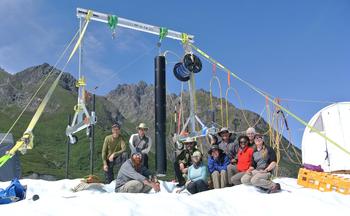
Fig. 1. The VALKYRIE cryobot (black cylinder) and the 2015 field team deployed on the Matanuska Glacier, Alaska (61°42′09.3″N 147°37′23.2″W) from 9 June to 10 July 2015.
Motivations for autonomous sampling
Two challenges facing scientific robots operating in remote environments are the difficulty of real-time control by a human operator and the limitations of finite resources aboard the robot. Because VALKYRIE carries a limited number of sample bags (12 maximum) and the ice profile encountered during the descent is unknown a priori, these challenges manifest themselves in the question of how to intelligently choose when to take water samples. Because the presently observed sample water will mix with the contaminated water trailing VALKYRIE's descent and the sample bags are one-time-use to prevent contamination, the decision to take a sample is irrevocable. VALKYRIE can neither backtrack to take a high value sample it saw in the past, nor give up a sample it has already taken if it sees something better in the future.
During the field campaign, most water samples were remotely triggered by a human science team monitoring science telemetry for signals of interest from the surface. During planetary missions or missions in extreme environments on Earth, however, time delays, sparse communication windows and limited human endurance preclude such supervision. In order to maximize science return, it is necessary for the robot to make intelligent autonomous decisions about how and when to expend its resources. The algorithm responsible for making these decisions must be adaptive enough to account for great uncertainty about what will be encountered in a fundamentally unknown environment.
This paper discusses the development of two algorithms for intelligent autonomous water sampling aboard the VALKYRIE cryobot. The first algorithm presented (Algorithm 1) was developed during the 2015 field campaign and was used to autonomously collect a suite of water samples in real time during an active mission. The second algorithm (Algorithm 2) improves upon the first algorithm given lessons learned from the field. The performance of both algorithms is compared using both simulated data and real data from the field, and is shown to be on par with human performance. Finally, we discuss applications of the VALKYRIE autonomous sampling algorithm and address implications of our results to autonomous and agile science applications in general.
Related work
The development of algorithms for agile science and autonomous exploration has been pursued with much interest in contexts ranging from spacecraft to planetary rovers to unmanned aerial vehicles to autonomous underwater vehicles, and these algorithms have been shown to substantially improve science return (Thompson et al. Reference Thompson2012). Yet truly autonomous behaviour remains challenging to achieve in operational situations because such capacities require deep systems-level integration and high confidence in proper behaviour of the algorithm in the face of inherently unknown environments. Successes have been reported for Earth observing spacecraft (Chien et al. Reference Chien2015), spacecraft performing flybys of primitive bodies (Chien et al. Reference Chien, Knight, Stechert, Sherwood and Rabideau1999, Reference Chien2014), planetary rovers on Earth and Mars (Gulick et al. Reference Gulick, Morris, Ruzon and Roush2001; Wagner et al. Reference Wagner2001; Castano et al. Reference Castano2007b; Woods et al. Reference Woods2009) and autonomous underwater vehicles (Smith et al. Reference Smith2011; Girdhar et al. Reference Girdhar, Giguère and Dudek2013). In many cases, the vehicles were able to actively modify their trajectory to improve observations or facilitate direct interactions with their environment as new science opportunities were discovered, while still maintaining high-level mission directives from ground control.
When striving towards intelligent autonomy for robotic science, the question naturally arises: What constitutes valuable science? Many previous works concentrate on implementing onboard intelligence for a single, well-focused science task. Examples include a vision-based Bayesian classification system for identifying rock types observed by a planetary rover (Sharif et al. Reference Sharif, Ralchenko, Samson and Ellery2015), and a support vector machine trained to taxonomically identify plankton cells passing through an imaging flow cytometer deployed at a cabled coastal ocean observatory (Sosik & Olson Reference Sosik and Olson2007). These observations could then be used to guide science directives for the vehicle or other deployed science assets.
Other works take a more generalistic approach, guiding science directives with the ‘principle of most surprise’ – that is, the idea that what is most scientifically interesting in an environment is also what is most surprising, and the vehicle should actively seek this out. Kaeli (Reference Kaeli2013) describes a methodology for categorizing visual observations of the environment into topics based on semantic descriptors and provides a quantitative framework for the metric of surprise. Girdhar et al. (Reference Girdhar, Giguère and Dudek2013) extend these ideas by implementing an online topic modelling-based algorithm in an autonomous underwater robot, continuously computing the surprise score of the current observation, and executing an intelligent traversal strategy including hovering over surprising observations while moving quickly over corals and rocks similar to those previously seen. Castano et al. (Reference Castano2007a) tackle the problem of novelty detection on rock images acquired by a wheeled rover through several strategies – k-means clustering on rock properties, a probability-based Gaussian mixture model, and a discrimination-based single classifier approach – and incorporate these capabilities into a closed-loop system for autonomous rover science including opportunistic investigation of science targets and online replanning subject to vehicle resource constraints.
Problem formulation
VALKYRIE may continually measure the protein and mineral concentrations of the meltwater during descent using its flow cytometer, and at any time choose to collect the meltwater into a limited number of sample bags or sample filters. We assume in the following sections that VALKYRIE is configured pre-mission with 12 empty sample bags (the maximum it can hold). The objective of the autonomous sampling algorithm is to enable VALKYRIE to collect the most scientifically valuable water samples without human guidance. VALKYRIE may choose to take a sample only in the present moment – it may not go back to retrieve a sample it has seen in the past, or discard a sample it has already taken and replace it with a better sample it sees in the future.
Because science ‘value’ is entirely subjective on the desires of the mission scientists for each particular campaign, we do not attempt to pass judgement on science value within the autonomous sampling algorithms themselves. Instead we assume that the scientists have implemented a ‘score function’ that provides a mapping from robot sensor readings to the expected scientific value of collecting a sample. More specifically, the score function performs sensor fusion and outputs a scalar representing the expected scientific merit of collecting a sample at the current timestep according to the science objectives. We require the output of this mapping as a pre-requisite input to the autonomous sampling algorithms.
Given a score function mapping, the sampling problem reduces to picking the twelve globally highest scoring samples while the score function output is gradually revealed as the mission progresses, under the constraints that samples may be triggered only at the present timestep and each sample takes a discrete amount of time to complete. After a mission, once the whole score function has been observed, the optimal sampling times may be calculated by brute force. Generally speaking, the metric for measuring performance of an online algorithm is called the competitive ratio (Manasse & McGeoch Reference Manasse and McGeoch1988), defined as the ratio of between the score of the solution found by the online algorithm and the score of the optimal a posteriori solution. We calculate the competitive ratio of a single run of the autonomous sampling algorithm as the sum of sample scores picked by the autonomous sampling algorithm, divided by the sum of optimal sample scores computed with a fully observed score function. We compare the performance of the two candidate algorithms using aggregate statistics of their competitive ratios when tested against an identical set of 2000 simulated missions, and against human performance on a smaller subset of these simulated missions.
Water sampling system specifications
When VALKYRIE is not using its water jets to assist melting, it may sample an uncontaminated meltwater pocket generated immediately in front of its nose during the descent (Clark et al. Reference Clark2017). In non-jetting mode, VALKYRIE passively melts through the ice using thermal inequilibrium. Because there are no disturbances, the physical tolerances between the ice shaft and the vehicle body are very tight. Because the downwards passage of the vehicle constantly generates new meltwater, the meltwater pocket is under positive pressure proportional to the descent rate of the vehicle and remains uncontaminated by the contents of the water column higher up or impurities from the surface. So long as the intake rate is less than the rate of meltwater generation, the vehicle may sample water representative of the slice of ice that it is currently passing through using a sampling inlet at the nose. If the intake rate exceeds the rate of meltwater generation, the vehicle will begin pulling in dirty ‘bathtub’ water that has already been contaminated by its passage and mixed with the rest of the water column.
A custom-made Leiden Measurements Technologies deep ultraviolet fluorescence flow cytometer enables VALKYRIE to analyse the protein and mineral concentrations in the meltwater in real time during descent. A sampling pump draws water from the uncontaminated meltwater pocket via the sampling inlet, and passes it through a quartz window. As the water passes through the window, it is energized by a ultraviolet light source. A series of photomultiplier tubes (PMTs) tuned to different frequencies measure the fluorescence response of any material suspended in the water, and software performs least-squares chemometric fitting based on a series of predefined basis sets to quantify the concentration of chlorophyll A and various other proteins and minerals and logs the data in real time.
Once the meltwater passes through the quartz window for analysis by the cytometer, VALKYRIE has the options of letting the water pass out the back of the vehicle uncollected or redirecting it into a bank of ThermoScientific HyClone Labtainer BPC 100 ml sample bags (overfilled to 120 ml) or Pall 0.2 µm pore-size 90 mm diameter filters loaded into a Savilex filter holder. Upon post-mission recovery of the vehicle to the surface, the sample media are extracted for intensive laboratory analysis. There exists a 137 ml delay line between the quartz window and the sampling valve, so it is possible to view the entire contents of a 120 ml sample bag before deciding to collect it. A 40 µm ‘gunk filter’ is present at the sampling inlet to prevent ingestion of large particulates and a ‘bubble trap’ containing a 150 µm filter and an air escape pathway is incorporated to prevent air bubbles from entering the sample lines. The sampling pump is a magnetically coupled magnetic gear pump that was chosen to maximally isolate the sample contents from pump mechanicals while still satisfying the performance demands of the downstream system in terms of pressure.
Candidate algorithms
Algorithm 1 (field campaign algorithm)
The autonomous water sampling algorithm used in the VALKYRIE 2015 field campaign (Algorithm 1) uses an adaptive sample threshold to adjust its standards of what constitutes an ‘interesting’ sample during a mission and determine good moments to collect water samples. First, the sample threshold is initialized to a baseline value. During the field campaign, this baseline was anecdotally chosen to be slightly higher than the average steady-state score function value observed at the start of recent previous missions in nearby melt holes. Whenever the sample score surpasses the sample threshold, the algorithm commits to collecting a sample. It does not take the sample immediately, but waits to trigger sampling until a peak is reached in the score function in order to maximize the local score while the score function is still increasing. At the moment of triggering, the sample threshold is raised to twice the current sample score, and a depth threshold is put in place. Further sample triggering is prevented until the robot depth surpasses the depth threshold. Once the depth threshold is passed, sample triggering is re-allowed. After this, the sample threshold decays exponentially at a rate proportional to the time since the last sample and the number of samples remaining, and inversely proportional to the depth remaining before the end of the mission, down to the initial threshold value, or the score function exceeds the threshold again. If the algorithm reaches a point where there is less time remaining in the mission than the minimum amount of time needed to fill the remaining empty sample bags, then it immediately attempts to fill all remaining bags by sampling continuously.
At a high level, the idea behind Algorithm 1 is that the sampling threshold quickly adjusts upwards to a ‘reasonable’ threshold by exponential doubling whenever a sample is taken, and also adjusts downwards through exponential decay if high scores were seen in the past, but are no longer being seen. In essence, the algorithm is adjusting its expectation of what constitutes an interesting sample based on the score of the last sample and the amount of time that has passed since taking it. Pseudocode for Algorithm 1 is presented in Appendix I.
Algorithm 2 (improved algorithm)
A second autonomous sampling algorithm (Algorithm 2) was designed as an improvement over Algorithm 1, given the lessons learned from the 2015 field campaign. One major limitation of Algorithm 1 is that good performance requires tuning of several parameters such as initial sampling threshold and threshold decay rate. During the 2015 field campaign, Algorithm 1 could be tuned anecdotally because an environmental baseline was known ahead of the autonomous mission from previous missions conducted nearby. In environments with a truly unknown baseline, Algorithm 1 may perform poorly because these parameters are set inappropriately. Algorithm 2 is designed to be parameterless to avoid this major weakness of Algorithm 1.
The VALKYRIE sampling problem may be seen as a variation on the famous secretary problem in optimal stopping theory. Algorithm 2 draws heavily on inspiration from prior work on this subject. Simply stated, the secretary problem is as follows: suppose that you manage a company, and you wish to hire the best secretary from a pool of n applicants. Unfortunately, you cannot tell how good each applicant is until you interview them, and you must decide whether or not to make an offer immediately upon conclusion of the interview. Assume that all applicants will accept your offer, thus the hiring process halts as soon as you make your first offer. Because your decision is irrevocable, you will have to hire a secretary before observing the quality of applicants that have not yet been interviewed. What is the best strategy to choose which applicant to hire?
In 1961, Lindley suggested the following approach: Given n applicants, interview the first n/e applicants as a calibration period without hiring anyone. Then hire the first applicant who is as good or better than the best applicant from the calibration period. If you reach the last applicant without hiring anyone, hire that applicant no matter what (Lindley Reference Lindley1961). Papers by Chow & Robbins (Reference Chow and Robbins1963) and Dynkin (Reference Dynkin1963) proved that the probability of selecting the best applicant using this strategy asymptotically approaches 1/e as n grows large, and that the generalized strategy is optimal, yielding the best possible guarantee.
Further work in this field has explored variations on the secretary problem including picking different numbers of secretaries (the k-choice secretary problem), selecting multiple secretaries such that their individual strengths and weaknesses create the best team (the matroid secretary problem) and selecting a secretary when the value of that secretary is also partially dependent on the time it took to arrive at that decision (the time discounting secretary problem). Babaioff et al. (Reference Babaioff, Immorlica, Kempe and Kleinberg2008) presents a comprehensive review on approaches to these problems, and observes surprisingly strong constant factor guarantees on the expected value of solutions obtained from generalized online secretary algorithms.
For the VALKYRIE sampling algorithm, the most relevant variation is the k-choice secretary problem. Given a scoring function that continuously measures the anticipated utility of taking a sample at any given point in time, the VALKYRIE sampling problem may be approximately reduced to the k-choice secretary problem, except that the scores of the secretaries are no longer independent of the secretaries that came before them, and after picking a secretary you must wait for a constant number of candidates before choosing the next.
Babaioff et al. describe a simple and intuitive algorithm for the k-choice secretary problem that is e-competitive as n approaches infinity, meaning it selects the best k applicants with probability 1/e for large n (Babaioff et al. Reference Babaioff, Immorlica, Kempe and Kleinberg2007). Kleinberg presents a more complicated recursive algorithm that is  $1 - 5/\sqrt k $ competitive, which provides a better competitive ratio for large k (Kleinberg Reference Kleinberg2005). We draw upon ideas from both these algorithms as inspiration for Algorithm 2.
At a high level, Algorithm 2 recursively divides the mission into smaller and smaller sub-missions and attempts to select a portion of its total samples from each smaller sub-mission. Like Algorithm 1, Algorithm 2 keeps track of a sampling threshold, but in this case, the sampling threshold is set as the mean value of all sub-missions that came before. As in Algorithm 1, Algorithm 2 commits to collecting a sample once the threshold is passed, but waits until a peak is reached in the scoring function to actually trigger the sample. Similarly, Algorithm 2 immediately takes all samples needed to fill its quota for a given sub-mission if it senses it is about to run out of time. Pseudocode for Algorithm 2 is presented in Appendix II.
Figure 2 shows a visualization of the execution of both algorithms on the same simulated mission example, as well as the optimal sampling times computed post-mission when the entire score function is known. It can be seen that the setting of the exponential decay rate is very important to the performance of Algorithm 1, and that Algorithm 1 is good at picking peaks of local spikes in the score function, but usually misses the opportunity to take multiple samples in a drawn-out region of high score function values. In this example, Algorithm 2 outperforms Algorithm 1, with a competitive ratio of 0.911 versus 0.800, respectively.

Fig. 2. Illustration of execution of both autonomous sampling algorithms on identical simulated mission data. The solid blue line represents the score function. Gold stars show optimal samples computed with a priori knowledge of the score function for the entire mission. Red triangles show samples picked by Algorithm 1 and green dots show samples picked by Algorithm 2. Dashed lines represent the sampling threshold for each algorithm. Shaded regions show times when the sampler is sampling.
Analysis of performance
Performance comparison on simulated data
In order to investigate algorithm performance with statistically significant sample sizes, Algorithm 1, Algorithm 2 and human performance were compared against each other when run against the same suite of 2000 mission simulations (human performance was tested on a smaller subset of these simulations). Individual mission simulations were generated by modelling the score function as a randomized Gaussian mixture model under the assumption that events of interest have a physical region of influence in the ice (which may overlap with other events of interest), and as the robot descends through these physical regions, the interestingness of the events it is passing through will be reflected in the score function. The parameters for the Gaussian mixture model generating the mission simulations were maximum event amplitude a max, number of Gaussian events n, maximum event width σmax (standard deviation) and length of mission L. For exact methodology of simulated mission generation, see Appendix III.
To gauge the effects of diverse mission morphologies on algorithm performance, one parameter of the Gaussian mixture model generating the mission simulations was varied at a time, and the algorithms were tested on resultant mission simulations (e.g. How does the mission length affect the algorithm's ability to pick the optimal samples?). Although not part of the Gaussian mixture model, the number of samples to collect s was also varied. Fifty trials were performed per parameter configuration for Algorithms 1 and 2, and five trials for humans in the interest of practicality of human testing. Parameter values when being held constant were n = 50 events, s = 12 samples, σ max = 25, mission length L = 500. When varying mission length, the number of events was instead scaled to maintain the default proportion 50/500 in order to correspond to what would happen in real life. Maximum event amplitude a max was not varied and was arbitrarily fixed at 50 because the score function is unitless.
Algorithm performance was measured using the competitive ratio – the ratio of total sample score picked by the algorithm over the optimal score. Optimal samples were estimated using a priori knowledge of the entire score function using a greedy algorithm (see Appendix IV). Because we are interested in studying best-case performance, parameters for Algorithm 1 (baseline sampling threshold m and threshold decay rate r) were tuned by hand to produce the best aggregate results, but were not modified across mission simulations. Human performance was measured by gradually revealing an animated plot of the score function to a human user and having them press a computer key whenever they desired to collect a sample. The animation frequency of score function updates during human trials was 5 Hz.
Both algorithms perform well on simulated data with a one σ competitive ratio range of 0.6–0.85 for most mission configurations. They show performance on par with human performance and would likely significantly exceed human performance on long missions when a human's attention will inevitably wander (the longest simulated missions tested took about 5 min to complete by humans per trial – during the VALKYRIE field deployment, missions could stretch upwards of 16 h). Both algorithms exhibit good stability when run against diverse missions morphologies constructed from simulation parameters with a wide range of the number of Gaussian events, maximum event width, number of samples and mission length – that is, their performance stays relatively constant as these parameters are varied.
Some variation is observed, however. For conciseness, let the phrase ‘all algorithms’ include human performance. The performance of all algorithms is relatively flat as the number of Gaussian events is varied, except it is worse at very low numbers of Gaussian events. This is likely because when the number of Gaussian events is similar or smaller than the number of samples, there is a higher penalty for mistakenly skipping a good event. By the pigeonhole principle, there are not enough other decent events to make up for it, so the algorithm is forced to spend a sample at an inopportune time. All algorithms perform better as the number of samples increases. This is likely because the more samples are available, the better coverage the algorithm can make of the mission, regardless of its morphology. If an algorithm was able to achieve 100% sampling coverage of a mission, by definition it would achieve an optimal sampling routine. Having more samples available drives the algorithms towards this scenario. Algorithm 2 and humans show poor performance at very small maximum event width. Humans perform poorly because their reflexes are not fast enough to catch very narrow events going by. Algorithm 2 performs poorly because the narrowness of these events means they have a small integral, so they do little to influence the sampling threshold, thus Algorithm 2 has a hard time initializing its threshold well. Algorithm 1 does decently in this scenario, but with the caveat that it has the unfair advantage of prior information due to the manual pre-initialization of its sampling threshold. Beyond a certain small maximum event width, all algorithms perform decently and performance flattens out. This is likely because very wide events essentially contribute a constant offset to the background baseline of the score function, and constant offsets do not affect the algorithms (beyond the initialization of Algorithm 1), because score functions are unitless. Finally, Algorithm 2 performs markedly better than Algorithm 1 as the missions get longer. This is likely because the sampling threshold decay rate in Algorithm 1 becomes poorly tuned for the longer mission lengths. This illustrates the benefits and flexibility of Algorithm 2's parameterless nature.
Overall, Algorithm 2 slightly outperforms Algorithm 1 in almost all cases, and has the major advantage that it requires no tuning to achieve good performance. Figure 3 shows the results of the sensitivity analysis investigating varied mission simulation parameters on the performance of the algorithms.

Fig. 3. Aggregate performance of Algorithm 1, Algorithm 2 and humans on a suite of 2000 simulated missions generated by a Gaussian mixture model (humans were tested on only a subset). Mission simulation parameters were number of Gaussian events, number of samples, maximum event width and mission length. One parameter of the mission simulation was varied at a time to investigate the effect of different mission morphologies on algorithm performance. Shaded area shows one standard deviation.
Autonomous collection of VALKYRIE field samples
The science objective for sampling during the VALKYRIE field campaign was to gather water samples during descent from regions in the ice with the largest concentration of biosignals, for which cytometer fluorescence signal was utilized as a proxy. The autonomous sampling score function used was the sum of the six cytometer PMT channel count rates computed at each timestep, convolved with a 120 ml box filter sampling window – the idea being that this number measured the total amount of fluorescent material that would end up in a sample bag if a water sample was triggered at the current moment in time.
Algorithm 1 was used to collect ten 120 ml sample bags autonomously during the final mission of the VALKYRIE 2015 field deployment. A networking error caused the algorithm to reset after the second sample, so the adaptive threshold was abnormally low for the third and fourth samples as the algorithm re-learned the environment. Despite the networking error, the algorithm collected a series of samples representing high score function values starting with no a priori knowledge of what would be encountered during the descent (competitive ratio 0.518). Cell concentrations for each sample bag were measured post-mission after the bags had been returned to the surface using the methodology described in Christner (Reference Christner2006). Only a modest correlation (r 2 = 0.23) was observed between the score function value and the laboratory-processed cell concentration, implying that the score function used did not provide a reliable translation between sensor readings and actual concentration present in the water samples. The discrepancy is due to a sub-optimal choice of score function, not the performance of the algorithm itself, and is not wholly unexpected given that the score function consisted simply of a naive measurement of total fluorescent signal contained in each water sample (the sum of all PMT channels across a 120 ml window). The poor correlation may have had to do with non-biological sources of fluorescence in the sample water or high concentrations of cells passing through the cytometer in clusters instead of well mixed in the sample water, among other factors. Future work will address this discrepancy by analysing the VALKYRIE data to determine a more appropriate sensor fusion that accurately represents the sample's cell concentration. The improved score function may use more sophisticated techniques such as chemometric fitting to extract the concentrations of particular biomarkers of interest instead of just generic fluorescent activity. An important contribution of the VALKYRIE vehicle was to gather this baseline dataset from a representative field environment, so that these analyses may be completed and a more accurate score function can be constructed in the future for this and other scientific objectives. Figure 4 shows the autonomous samples collected by the VALKYRIE vehicle during the 2015 field campaign and the correlation between score function value and sample cell concentration as measured in the sample water post-mission upon retrieval of VALKYRIE from the borehole.

Fig. 4. Plot showing the response of the water sampling algorithm during the 5 July 2015 autonomous mission on the Matanuska Glacier (left). Ten sample bags were collected autonomously during this mission and were retrieved for laboratory analysis upon resurfacing of the vehicle at the conclusion of the mission. Correlation between score function and cell concentration was r 2 = 0.23 (right). The data point representing the third sample was thrown out because the communications error with VALKYRIE caused the sampling pump to stop and be reset, which mixed sample water from different depth layers in the ice.
Algorithm performance comparison on VALKYRIE field data
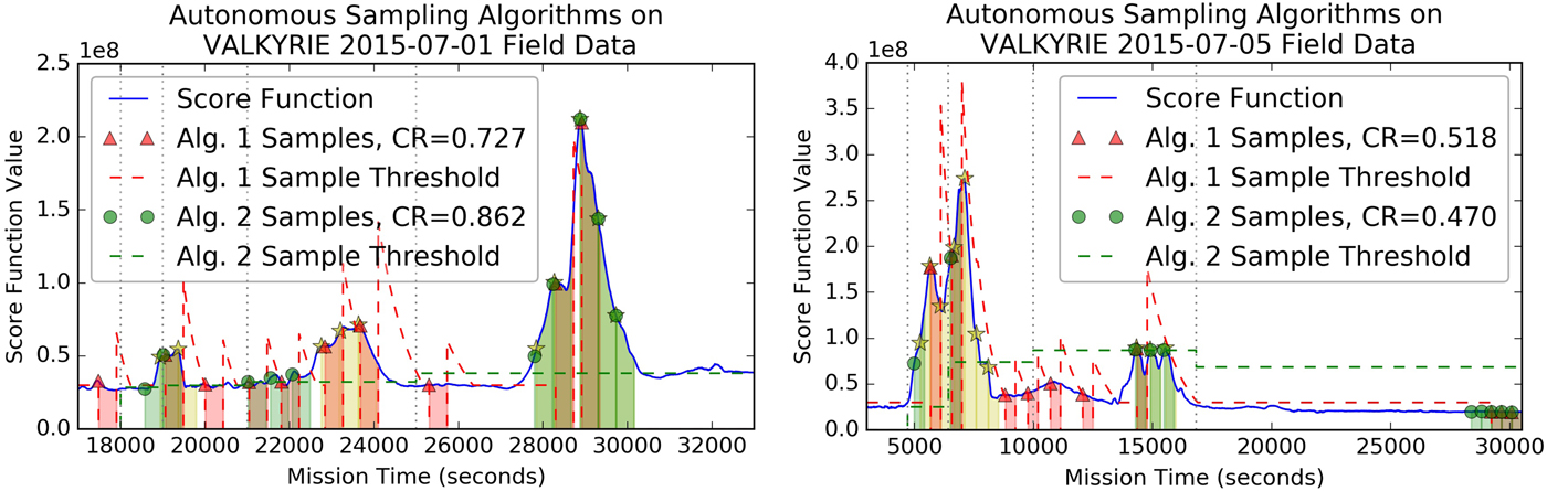
Because Algorithm 2 was not developed until after the VALKYRIE 2015 field campaign, both Algorithm 1 and Algorithm 2 were run after the fact on historical 2015 field deployment data (and parameter settings, in the case of Algorithm 1) to compare performance. Figure 5 shows the performance of both algorithms on 1 July and 5 July 2015 mission data. The samples, chosen by Algorithm 1 during the re-run, are not exactly the same as those chosen during the field mission because of the networking error in the field mission that caused Algorithm 1 to reset midway through the mission. Both algorithms performed better on the July 1 mission data than the July 5 mission data, which is to be expected because the July 1 mission was back-loaded (had its highest score function values near the end), whereas the July 5 mission was front-loaded (had its highest score function values near the beginning). If a mission is front-loaded, the algorithm can have little certainty that the high scores it sees near the beginning are the best in the mission, because it has yet to observe the remainder of the mission. If a mission is back-loaded, it can have better certainty that high scores near the end are indeed the best thing it will see, which leads to better performance. Algorithm 2 outperformed Algorithm 1 in the July 1 mission because it was better able to sample broadly across the large late high-scoring event, instead of only picking out the peaks like Algorithm 1. Algorithm 1 did better on the July 5 mission because it sampled frequently early in a front-loaded mission, whereas Algorithm 2 waited for something better to come along, then was forced to desperately take five poorly scoring samples at the end to fill its quota. Probabilistically, Algorithm 2 made the better choice to wait as evidenced by its superior aggregate performance on large collections of simulated missions. However, in the case of the July 5 mission, it turned out that the large early score function spike was the best available region for sampling. Anecdotally, both algorithms were more reliable and precise than human operators, who could not constantly monitor the science telemetry during the entire 7+ hour duration of these missions.

Fig. 5. Plot showing the response of the autonomous water sampling algorithms run on data from VALKYRIE 2015 field deployment to the Matanuska Glacier. The solid blue line represents the score function. Gold stars show optimal samples computed with a priori knowledge of the score function for the entire mission. Red dots are samples picked by Algorithm 1 and green dots show samples picked by Algorithm 2. Dashed lines represent the sampling threshold for each algorithm. Shaded regions show times when the sampler is sampling.
Conclusions
Two algorithms were developed to solve the challenge of autonomous scientific water sampling aboard the VALKYRIE cryobot during descent through a glacier. The first algorithm (Algorithm 1) was used to autonomously collect ten water samples with high relative cell concentrations during the final mission of the VALKYRIE 2015 field campaign. The second algorithm (Algorithm 2) was developed after the field campaign and improved upon Algorithm 1 given lessons learned in the field. The performance of both algorithms was characterized and compared over a wide range of mission morphologies using simulated data, and found to have good performance and stability across different mission types. The algorithms perform on par with human performance during simulated missions, and would perform better than humans on long missions in the field due to the algorithms’ ability to monitor tirelessly and indefinitely. Algorithm 2 outperforms Algorithm 1 and is more robust to varied mission morphologies because it is parameterless and requires no tuning. The dataset gathered during the VALKYRIE 2015 field campaign will assist in the formulation of more accurate score functions (sensor fusions) that map instrument data to scientific value towards mission objectives.
The development of autonomous sampling algorithms opens up many operational possibilities for VALKYRIE or its technological descendants to perform long-duration science operations in environments too extreme for continuous human oversight. Examples include missions that penetrate Greenlandic or Antarctic ice sheets to access sub-glacial lakes, or eventually planetary missions to icy ocean worlds like Europa or Enceladus. The ideas developed in Algorithms 1 and 2 are not limited to application on cryobots, but are applicable to any situation requiring intelligent utilization of limited resources with an uncertain future. These ideas could be extended to other robotic exploration platforms, selective data return in bandwidth limited situations, sports betting, stock trading and more.
Acknowledgements
This work was supported by NASA ASTEP programme grant NNX11AJ89G, PI Bill Stone. The authors would like to thank the NASA ASTEP programme for making this work possible.
Appendices
Appendix I: Algorithm 1
Fig. A1. Pseudocode for Algorithm 1, the autonomous sampling algorithm used during the 2015 VALKYRIE field campaign.
Appendix II: Algorithm 2
Fig. A2. Pseudocode for Algorithm 2, the improved algorithm designed after the field campaign.
Appendix III: generation of mission simulations
Mission simulations were generated using a Gaussian mixture model – a sum of Gaussians, where each Gaussian's amplitude a, centre (mean) μ and width (standard deviation) σ were chosen uniformly randomly from within a pre-set range. The parameters for the Gaussian mixture model are: maximum event amplitude a max, number of events n, maximum event width (standard deviation) σ max and mission length L. The thinking behind this model is that as VALKYRIE descends through the glacier, it randomly encounters impurities in the ice that contribute to the cytometer fluorescence signal. The amplitude and duration of each impurity's contribution is unknown, so the region of influence is modelled as Gaussian. The regions of influence of the impurities can overlap, so the aggregate fluorescence measured by the VALKYRIE cytometer is the sum of these Gaussian regions of interest. This approach proved to be a decent model for generating realistic mission simulations, and was able to produce a rich morphological variety of mission simulations that were anecdotally similar to measurements gathered from the 2015 VALKYRIE field campaign. One weakness of the model is that in the field, impurities were generally observed to be somewhat clustered instead of uniformly distributed. The pseudocode for generating a single mission simulation given the parameters of the Gaussian mixture model is shown below.
Fig. A3. Pseudocode for generation of mission simulations using a Gaussian mixture model.
Appendix IV: greedy algorithm for estimating optimal samples post-mission
The calculation of competitive ratio requires knowledge of the optimal sampling score, so an algorithm is needed that can compute the optimal sampling score, given a priori fully observed mission. Although it is difficult to compute a truly optimal score, especially for long missions because the number of sampling permutations that would have to be tried is large, the following greedy algorithm presented in Fig. A4 correctly calculates the optimal samples in almost all cases. One example where the optimal sample estimation fails is shown in Fig. A5. In this case, the optimal sample estimation underestimates the optimal score, which would lead to an overestimation of the competitive ratio. Although this is possible in theory, in practice it is highly unlikely to occur and is therefore lost to noise when averaged across many trials as were conducted during the performance analysis of the algorithms.
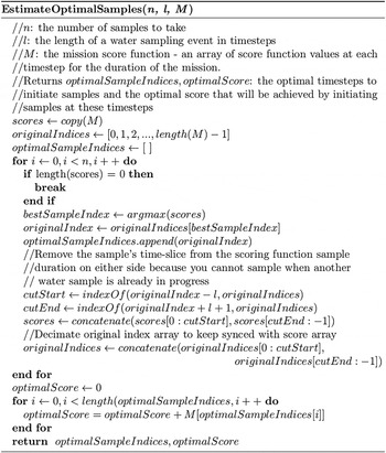
Fig. A4. Pseudocode for estimating optimal samples from a mission when the entire mission is observable a priori.

Fig. A5. Example where the greedy optimal sample estimation algorithm fails. When a score function peak is close to twice the width of the sampling period, it may be more advantageous to take two sub-optimal samples on either side of the peak than one optimal sample at the peak and one very poor sample much below it.