2. THE RELEVANT EQUATIONS OF THE EULERIAN VLASOV CODE AND THE NUMERICAL METHOD

The relevant equations for the problem we are studying have been presented previously (see, for instance, Appendix B in Ghizzo et al., Reference Ghizzo, Bertrand, Shoucri, Johnston, Fijalkow, Feix and Demchenko1992 for more details). We rewrite these equations in order to fix the notation. Time t is normalized to the inverse electron plasma frequency ${\rm \omega} _{{\rm pe}}^{ - 1} $, velocity and momentum are normalized respectively to the velocity of light c and to M _ec, where M _e is the electron mass, length is normalized to ${l_0} = c{\rm \omega} _{{\rm pe}}^{ - 1} $, and the electric field is normalized to E ₀ = M _eω_pec/e. The 1D Vlasov equations for the electrons and ions distribution functions f _e,i(x, p _xe,i, t) verify the relation:

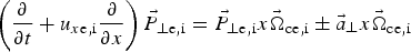
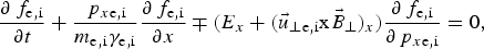(1)$$\displaystyle{{\partial {\,f_{{\rm e},{\rm i}}}} \over {\partial t}} + \displaystyle{{{\,p_{x{\rm e},{\rm i}}}} \over {{m_{{\rm e,i}}}{{\rm \gamma} _{{\rm e},{\rm i}}}}}\displaystyle{{\partial {\,f_{{\rm e,i}}}} \over {\partial x}} \mp ({E_x} + {({\vec u_{ \bot {\rm e},{\rm i}}}{\rm x}{\vec B_ \bot} )_x})\displaystyle{{\partial {\,f_{{\rm e},{\rm i}}}} \over {\partial {\,p_{x{\rm e},{\rm i}}}}} = 0,$$

where γ_e,i ≈ (1 + (p _xe,i/m _e,i)²)^1/2. The upper sign in Eq. (1) is for the electron equation and the lower sign for the ion equation, and subscripts e and i denote electrons and ions, respectively. In our normalized units m _e = 1, and m _i = M _i/M _e = 1836 is the ratio of ion to electron masses. In this 1D model, the transverse velocity ${\vec u_{ \bot {\rm e},{\rm i}}}(x,t)$ is assumed non-relativistic and is calculated from a transverse “fluid” equation, but the kinetic features of the plasma are fully preserved along the external magnetic field in the longitudinal direction x. The transverse momentum 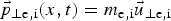${\vec p_{ \bot {\rm e},{\rm i}}}(x,t) = {m_{{\rm e},{\rm i}}}{\vec u_{ \bot {\rm e},{\rm i}}}$ is obtained through the introduction of the generalized canonical momentum defined by ${\vec P_{ \bot {\rm e},{\rm i}}}(x,t) = {\vec p_{ \bot {\rm e},{\rm i}}}(x,t) \mp {\vec a_ \bot} (x,t)$ ($\vec A$ is the vector potential of the wave, and $\vec a = e\vec A/{M_{\rm e}}c$ is the normalized vector potential), which obeys the “fluid” equation:

(2)$$\left( {\displaystyle{\partial \over {\partial t}} + {u_{x{\rm e,i}}}\displaystyle{\partial \over {\partial x}}} \right){\vec P_{ \bot {\rm e,i}}} = {\vec P_{ \bot {\rm e,i}}}x{\vec {\rm \Omega} _{{\rm ce,i}}} \pm {\vec a_ \bot} x{\vec {\rm \Omega} _{{\rm ce,i}}}$$

with 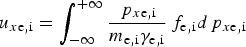${u_{x{\rm e,i}}} = \int_{ - \infty} ^{ + \infty} {\displaystyle{{{\,p_{x{\rm e,i}}}} \over {{m_{{\rm e,i}}}{{\rm \gamma} _{{\rm e,i}}}}}{\,f_{{\rm e,i}}}d{\,p_{x{\rm e,i}}}}$.

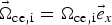${\vec{\rm \Omega}}_{{\rm ce},{\rm i}} = {{\rm \Omega}_{{\rm ce},{\rm i}}}{\vec e}_x$, where Ω_ce,i is the electron (ion) cyclotron frequency, and ${\vec e}_x$ is the unit vector in the direction of the external magnetic field.

We adopt the Coulomb gauge $\nabla \cdot {\vec a} = 0$, where the vector potential is in the perpendicular plane. The longitudinal electric field E _x is calculated either from the gradient of a potential E _x = −∂φ/∂x or from the Ampére's law:

(3)$$\displaystyle{{\partial {E_x}} \over {\partial t}} = - {J_x},\,\,{J_x} = \int_{ - \infty} ^{ + \infty} {\displaystyle{{{\,p_{x{\rm i}}}} \over {{m_{\rm i}}{{\rm \gamma} _{\rm i}}}}} {\,f_{\rm i}}d{\,p_{x{\rm i}}} - \int_{ - \infty} ^{ + \infty} {\displaystyle{{{\,p_{x{\rm e}}}} \over {{m_{\rm e}}{{\rm \gamma} _{\rm e}}}}{\,f_{\rm e}}d{\,p_{x{\rm e}}}.} $$

The transverse electric field ${{\mathop{E}^{\rightharpoonup}}_\bot} $ is calculated from the relations:

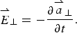(4)$${{\mathop {E}^{\rightharpoonup}}_\bot} = - \displaystyle{{\partial {{{\mathop {a} \limits^{\rightharpoonup}}}_ \bot}} \over {\partial t}}.$$

The transverse EM fields E _y, B _z and E _z, B _y for the circularly polarized wave obey Maxwell's equations. Defining E ^± = E _y ± B _z and F ^± = E _z ± B _y we have the following equations:

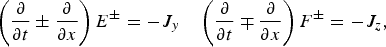(5)$$\left( {\displaystyle{\partial \over {\partial t}} \pm \displaystyle{\partial \over {\partial x}}} \right){E^ \pm} = - {J_y}\quad \left( {\displaystyle{\partial \over {\partial t}} \mp \displaystyle{\partial \over {\partial x}}} \right){F^ \pm} = - {J_z},$$

which are integrated along their vacuum characteristics x = ±t. In our normalized units, we have the following expressions for the normal current densities:

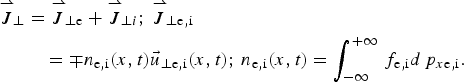(6)$$\eqalign{ {{{\mathop {J} \limits^{\rightharpoonup}} } _ \bot} & = {{{\mathop {J} \limits^{\rightharpoonup}}} _{ \bot {\rm e}}} + {{{\mathop {J} \limits^{\rightharpoonup}}} _{ \bot i}};\,{{{\mathop {J} \limits^{\rightharpoonup}} } _{ \bot {\rm e},{\rm i}}} \cr & \quad = \mp {n_{{\rm e},{\rm i}}}(x,t){{\vec u}_{ \bot {\rm e},{\rm i}}}(x,t);\,{n_{{\rm e},{\rm i}}}(x,t) = \int_{ - \infty} ^{ + \infty} {{\,f_{{\rm e},{\rm i}}}} d{\,p_{x{\rm e},{\rm i}}}.} $$

The numerical scheme applies a direct solution method of the Vlasov equation as a partial differential equation in phase space. This method has become an important method for the numerical solution of the Vlasov equation. In Eq. (1), γ_e,i ≈ (1 + (p _xe,i/m _e,i)²)^1/2 is a function p _x only, which allows us to apply a time-splitting scheme with the separation of x and p _x variables by a method of fractional steps, as discussed for Eulerian Vlasov codes in several publications (Shoucri & Storey, Reference Shoucri and Storey1986; Ghizzo et al., Reference Ghizzo, Bertrand, Shoucri, Johnston, Fijalkow and Feix1990, Reference Ghizzo, Bertrand, Shoucri, Johnston, Fijalkow, Feix and Demchenko1992; Shoucri, Reference Shoucri2008a).

3. TESTING THE CODE: PROPAGATION OF A LARGE AMPLITUDE WAVE

In this section, the response of the code is tested for large amplitude waves, in order to evaluate its precision and performance. Small amplitude perturbations of these waves will be used in Sections 4 and 5 for the SRS and SBS seed-pulse amplification problems.

3.1. The case of a forward scattering with a frequency of the laser pump ω_0P = 2.17, the electron cyclotron frequency Ω_ce = 1.4 and a vector potential for the pump a _0P = 0.09

We first test the code for a forward Raman scattering problem, where the forward injected large amplitude pump wave decays into another forward propagating wave and a plasma wave. We consider initially a Maxwellian plasma for the electrons and ions, with respective temperatures T _e = 0.3 keV and T _i = 0.02 keV. The ions do not play any role in the present physics, but have been included for the possible control of the small sheath at the edges. The linear dispersion relation for this problem is given by:

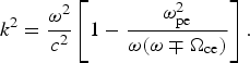(7)$${k^2} = \displaystyle{{{{\rm \omega} ^2}} \over {{c^2}}}\left[ {1 - \displaystyle{{{\rm \omega} _{{\rm pe}}^2} \over {{\rm \omega} ({\rm \omega} \mp {{\rm \Omega} _{{\rm ce}}})}}} \right].$$

The upper sign is for a right-hand circularly polarized wave (RCP), and the lower sign for a left-hand circularly polarized wave (LCP). The frequency of the EM wave is ω, and k the wavenumber. We consider a plasma such that the ratio of the electron cyclotron frequency Ω_ce to the electron plasma frequency ω_pe is Ω_ce/ω_pe = 1.4, and the ratio of the laser pump frequency ω = ω_0P to the electron plasma frequency is ω_0P/ω_pe = 2.17. In the remaining of the text, we will use only normalized values and write Ω_ce = 1.4 and ω_0P = 2.17. The corresponding wavenumber for the RCP wave calculated from Eq. (7) equals to 1.376, and equals to 2.025 for the LCP.

For the case of the forward Raman scattering problem under consideration, we have a forward propagating circularly polarized laser beam entering the system at the left boundary (x = 0), and the forward propagating fields of the circularly polarized constant amplitude pump are given at x = 0 by E ⁺ = 2E _0P cos (ω_0Pt) and F ⁻ = 2E _0P sin (ω_0Pt), where ω_0P = 2.17 and E ⁺ and F ⁻ are defined in Eq. (5). A characteristic parameter of high-power laser beams is the normalized vector potential or quiver momentum 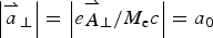$\Big\vert {{{{\mathop {a}^{\rightharpoonup}}}_\bot}} \Big\vert = \Big\vert {e{{{\mathop {A}^{\rightharpoonup}}}_ \bot} /{M_{\rm e}}c} \Big\vert = {a_0}$, where ${\vec A_ \bot} $ is the vector potential of the wave. For a circularly polarized wave $2a_0^2 = I{\rm \lambda} _0^2 /1.368 \times {\rm 1}{{\rm 0}^{{\rm 18}}}$, where I is the intensity in Wcm⁻² and λ₀ the laser wavelength in microns. We take the amplitude of the vector potential of the pump to be a _0P = 0.09, which is sufficiently high to excite the possible Raman scattered modes without having to add a perturbation for a stimulation. We have in our normalized units E _0P = ω_0Pa _0P. We use a system of length L = 800. The number of grid points in space is N = 120 000, so Δx = Δt = 0.00667. The extrema of momentum for the electrons are ±0.6, with 1300 grid points used in velocity space.

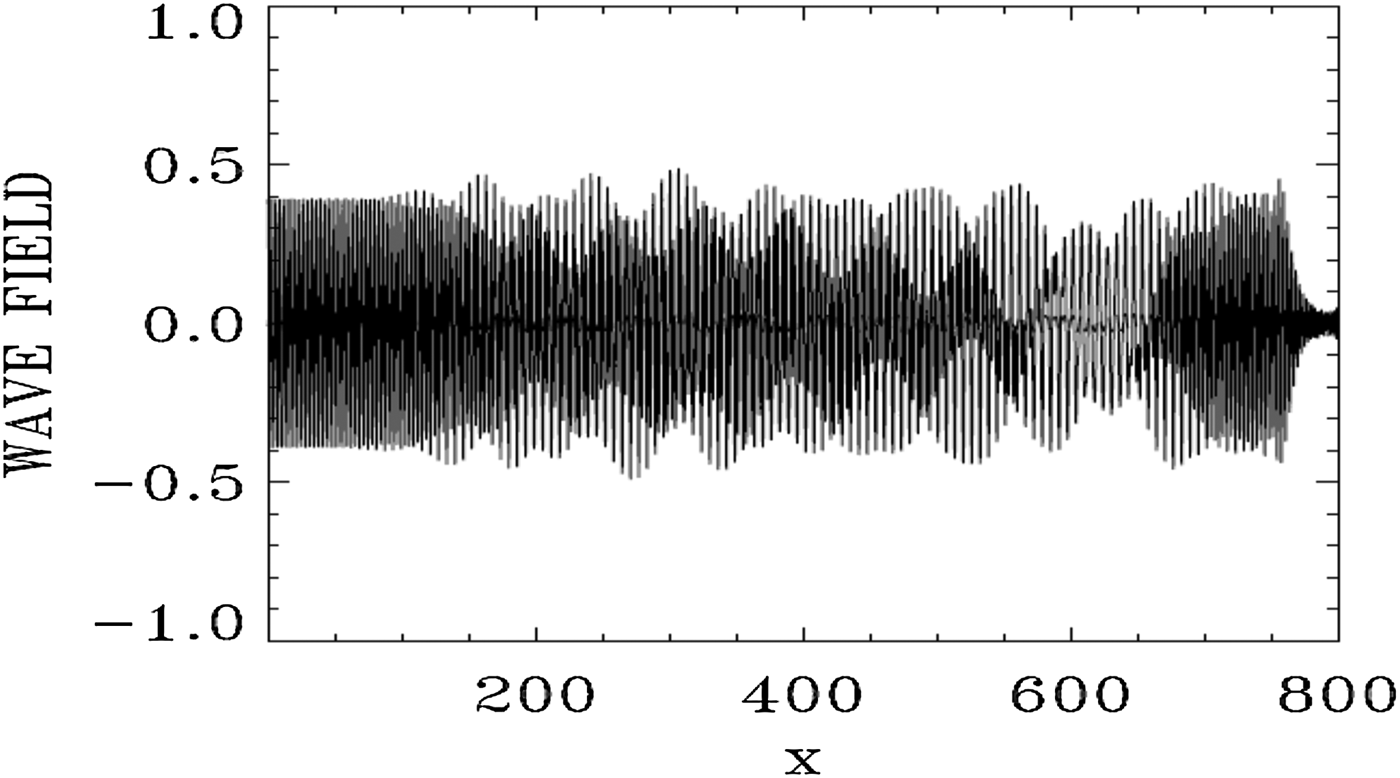
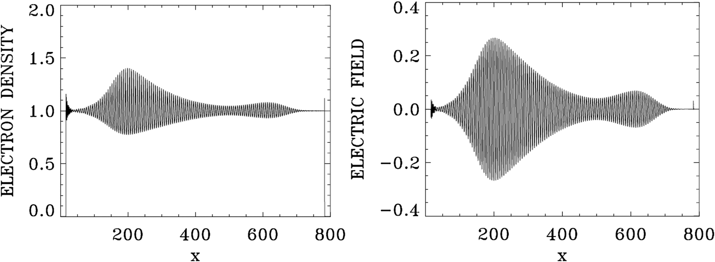
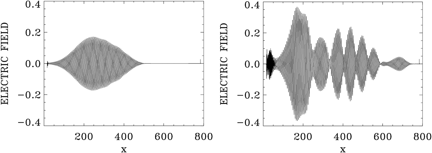
Figure 1 shows the forward EM wave E ⁺ at the time of the arrival of the signal precursor at the right boundary at t = 800. The wave consists of the initial injected pump (see the constant amplitude pump at the left in Fig. 1), beating with the forward Raman scattered modes (these modes will be analyzed in Figs 4 and 5 below). The pump appears to deplete (see the lighter part of the graphic around x = 600) and then grow again (darker part of the graphic after x = 700). Figure 2 shows the electron density and the electric field profiles at t = 800, and Figure 3 shows the phase-space contour plots of the electron distribution function at t = 800, at different position along the axis.

Fig. 1. The spatial profile of the forward wave E ⁺ at t = 800.

Fig. 2. Electron density and longitudinal electric field profiles at t = 800.

Fig. 3. Phase-space contour plots of the electron distribution function at different position in space at t = 800.

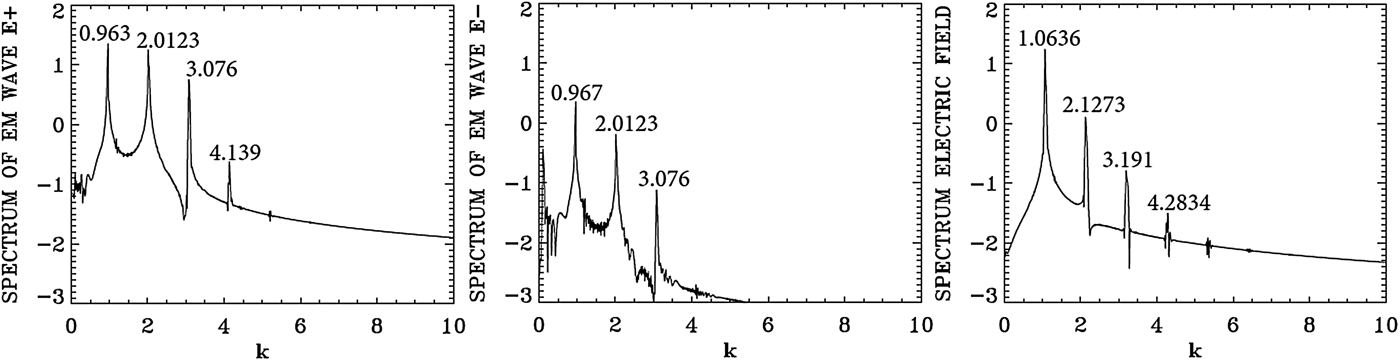
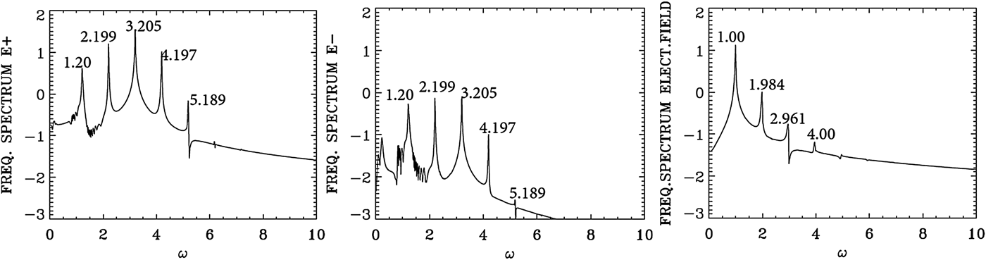
Fig. 4. Spatial Fourier transform in the domain x = (133,570) of the forward wave E ⁺, the backward wave E⁻, and the longitudinal electric field E _x at t = 800.

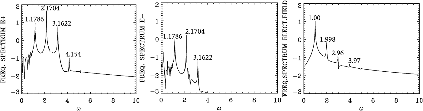
Fig. 5. Temporal Fourier transform, calculated in the time interval t = (266,704), for the forward wave E ⁺, the backward wave E⁻, and the longitudinal electric field E _x, taken at the position x = 200.

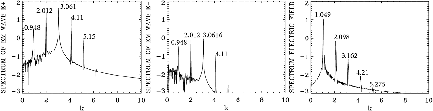
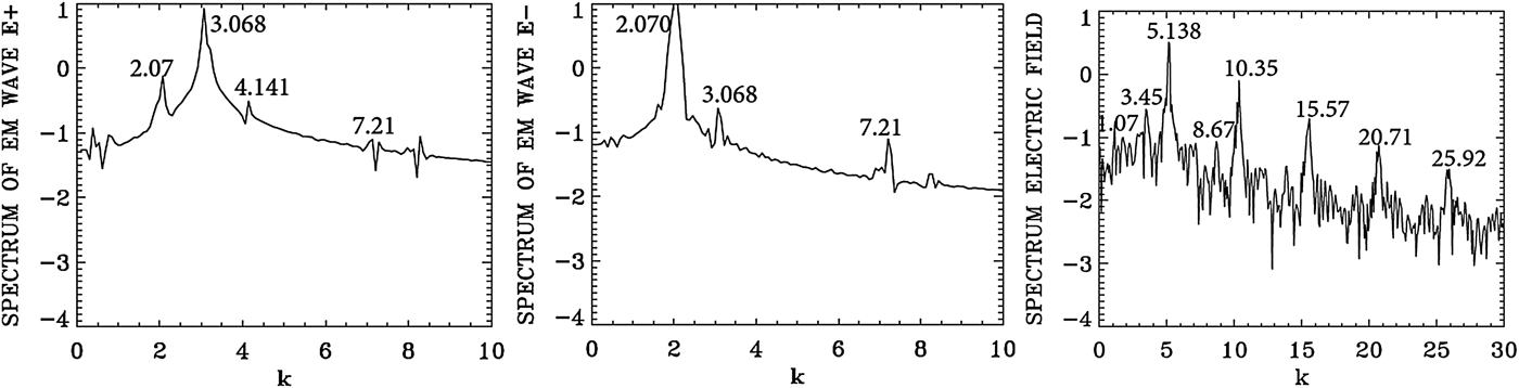
We present in Figure 4 the dominant spatial modes associated with the solution we present in Figures 1–3, by taking the Fourier transform in space for the forward wave E ⁺, the backward wave E ⁻ and the longitudinal electric field E _x in the domain x = (133, 570) at t = 800. Figure 5 presents the corresponding frequency spectra calculated by taking the temporal Fourier transform of the respective quantities in the time interval t = (266, 704), recorded at the position x = 200. Figure 5 shows for E ⁺ the dominant frequency of the laser at ω_0P = 2.1704, which is essentially the frequency 2.17 at which the pump is injected as we mentioned above. The wavenumber for E ⁺ in Figure 4 corresponding to this frequency is k _0P = 2.0123, in close agreement with the value of 2.025, which we calculated from Eq. (7) for ω_0P = 2.17 for a LCP [note that in the present simulation we are injecting a large amplitude wave, and the temperature effect has been neglected in the derivation of Eq. (7)]. So the injection of a laser pump with ω_0P = 2.17 at x = 0 has resulted in the excitation of a LCP wave with a wavenumber k _0P = 2.0123. We see in Figure 5 for the forward wave E ⁺ additional modes at frequencies 1.1786, 3.1622 and 4.154.

In free space, the forward wave E ⁺ and the backward wave E ⁻ are decoupled. In a nonlinear medium like the plasma, there is a weak coupling between E ⁺ and E ⁻ independent of the scattering process. This is the reason we observe in Figure 5 in the spectrum of E ⁻ peaks at the frequencies 1.1786, 2.1704, and 3.1622 at a much lower level compared with the level observed in E ⁺, and in Figure 4 we observe in the spectrum of E ⁻ peaks at the wavenumbers 0.967, 2.0123, and 3.076 at a much lower level compared with E ⁺.

The mode at ω_0F = 1.1786 in the frequency spectrum of E ⁺ in Figure 5 results from the forward Raman scattering of the pump according to the selection rule ω_0P = ω_0F + ω_e (where ω_e is the excited plasma frequency normalized to the electron plasma frequency ω_pe), from which we get for the excited plasma frequency ω_e = ω_0P − ω_0F = 2.1704 − 1.1786 = 0.9918, which is essentially the value of 1.00 we see in Figure 5 for the frequency spectrum of the electric field E _x (we note that the difference 1.00–0.9918 = 0.0082 is below the resolution of the Fourier transform, which is dω = 0.0144 in the present calculation). From Figure 4 the corresponding wavenumber of the forward scattered mode is k _0F = 0.963, in close agreement with the value of 0.965, we can calculate from Eq. (7) for ω_0F = 1.1786. It obeys the selection rule for the forward Raman scattering k _0P = k _0F + k _e, from which k _e = 2.0123 − 0.963 = 1.0493, very close to the value of 1.063 calculated in Figure 4 in the spectrum of the electric field E _x. From the plasma wave dispersion relation ${\rm \omega} _{\rm e}^2 = {\rm \omega} _{{\rm pe}}^2 + 3k_{\rm e}^2 {\rm \upsilon} _{\rm t}^2 $, written in normalized form as${\rm \omega} _{\rm e}^2 = 1 + 3k_{\rm e}^2 ({\rm \upsilon} _{\rm t}^2 /{c^2})$, where υ_t is the thermal velocity given in our normalized units for a temperature T _e expressed in keV by ${{\rm \upsilon} _{\rm t}}/c = 0.04424\sqrt {{T_{\rm e}}} $, and T _e is 0.3 keV in the present calculation. We get for the plasma frequency ω_e = 1.000, which is the result we see in Figure 5 in the frequency spectrum of the electric field E _x. Note that the backward Raman scattering k _0P = −k _0F + k _e is also possible, from which k _e = 2.0123 + 0.967 = 2.979, close to the harmonic at 3.191 in Figure 4. The corresponding frequency is ω_e = 1.00, which obeys the selection rule ω_0P = ω_0F + ω_e as discussed above. But the mode at 0.967 in the spectrum of E ⁻ in Figure 4 remained an order of magnitude smaller than the dominant modes in the spectrum of E ⁺. There is no other backward scattered mode excited by the pump.

Two more forward waves are excited for E ⁺, at the frequencies 3.1622 and 4.154 in Figure 5. This is essentially a cascade of LCP anti-Stokes resonance ω_0A1 = 3.1622 and ω_0A2 = 4.154. They obey the selection rule ω_0A1 = ω_0P + ω_e, from which ω_e = 3.1622 − 2.1704 = 0.9918, which is essentially the value of 1.0 we see in the frequency spectrum of the electric field in Figure 5. In a similar way ω_0A2 = ω_0A1 + ω_e, from which ω_e = ω_0A2 − ω_0A1 = 4.154 − 3.1622 = 0.9918. For the corresponding wavenumbers for the anti-Stokes modes, we can calculate from the dispersion relation for the LCP wave in Eq. (7) for ω_0A1 = 3.1622 the wavenumber 3.05, very close to the value of k _0A1 = 3.076 observed in Figure 4 for the spectrum of E ⁺ [note we are solving with a large amplitude mode and in the presence of a thermal spread, while Eq. (7) is a linearized dispersion relation]. It also obeys the selection rule k _0P = k _0A1 + k _e, from which the plasma mode wavenumber k _e = k _0P − k _0A1 = 3.076 − 2.0123 = 1.0637, which is essentially the value we can read in Figure 4 in the electric field spectrum frame. In a similar way for ω_0A2 = 4.154, we get from Eq. (7) the wavenumber 4.063, very close to the value of k _0A2 = 4.139 observed in Figure 4 for the spectrum of E ⁺. It obeys also the selection rule k _0A2 = k _0A1 + k _e, from which the plasma mode wavenumber k _e = k _0A2 − k _0A1 = 4.139 − 3.076 = 1.063, which is again the value we can read in Figure 4 in the electric field frame. We finally point out for the electric field in Figure 4 the harmonic structure of the wavenumber spectrum at 2.1273, 3.191, and 4.2834, and in Figure 5 the harmonic structure of the frequency spectrum at 1.998, 2.96, and 3.97. This is due to the large amplitude a _0P = 0.09 of the constant laser pump. Figure 2 shows large amplitude plasma waves.

3.2. The case of a forward scattering with a frequency of the laser pump ω_0P = 3.2, the electron cyclotron frequency Ω_ce = 0.5, and a vector potential for the pump a _0P = 0.07

We use the same parameters as in Section 3.1, except that for the pump laser beam we use a frequency ω_0P = 3.2 and a vector potential a _0P = 0.07, and we consider a plasma such that the normalized electron cyclotron frequency Ω_ce = 0.5. The corresponding wavenumber for the RCP wave calculated from Eq. (7) equals to 3.01, and equals to 3.062 for the LCP. Note the close values for these two wavenumbers for this lower value of Ω_ce = 0.5. Details of the injection of the pump at x = 0 are the same as in the previous section.

Figure 6 shows the forward EM wave E ⁺ at t = 533.3, and at the time of the arrival of the signal precursor at the right boundary at t = 800. The wave consists of the initial injected pump (see the constant amplitude pump at the left), beating with the forward scattered modes, which are excited without perturbation due to the high amplitude of the pump a _0P = 0.07 (these modes will be analyzed in Figures 7 and 8 below). The pump appears to deplete (see the lighter parts of the graphic) and then grow again (darker part of the graphic). These oscillations appear to be more regular at t = 533.3, with respect to what is presented at t = 800. Spatial Fourier transforms for E ⁺, E ⁻, and the longitudinal electric field at the early stage at t = 533.3 are presented in Figure 7, and provides the information about the modes which develop at this early stage. These transforms are calculated by Fourier transforming the signal in the interval x = (67,504) at t = 533.3. Figure 8 presents the corresponding frequencies calculated by a temporal Fourier transform of the signal at the position x = 200, in the time interval t = (233,452).

Fig. 6. The forward wave E ⁺ at t = 533.3 (left frame) and t = 800 (right frame).

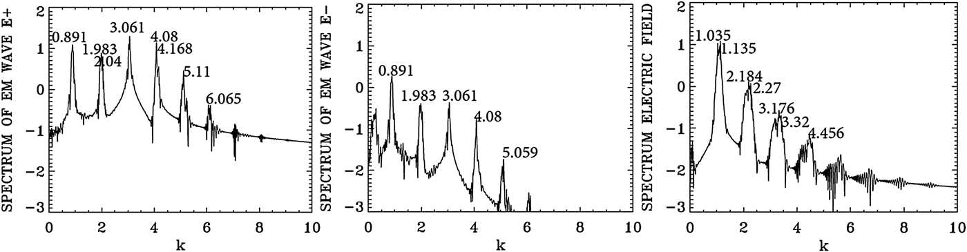
Fig. 7. Spatial Fourier transform in the domain x = (67,504) of the forward wave E ⁺, the backward wave E⁻, and the longitudinal electric field E _x at t = 533.3.

Fig. 8. Temporal Fourier transform, calculated in the time interval t = (233,452), for the forward wave E ⁺, the backward wave E⁻, and the longitudinal electric field E _x, taken at the position x = 200.

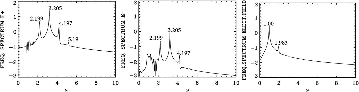
Figure 8 shows the dominant frequency for E ⁺ calculated by the code is at ω_0P = 3.205, which is essentially the frequency 3.2 at which the pump is injected as we mentioned above. The wavenumber for E ⁺ in Figure 7 corresponding to this frequency is k _0P = 3.061, in agreement with the value of 3.061 which can be calculated from Eq. (7) for ω_0P = 3.2 for a LCP. So the injection of a laser pump with ω_0P = 3.2 at x = 0 has resulted in the excitation of a LCP wave with k _0P = 3.061. We see in Figure 8 for the forward wave E ⁺ additional modes at frequencies 2.199, 4.197, and 5.19. The mode at ω_0F = 2.199 results from the forward Raman scattering of the pump according to the selection rule ω_0P = ω_0F + ω_e, from which we get for the excited plasma frequency ω_e = ω_0P − ω_0F = 3.205 − 2.199 = 1.006, which is essentially the value of 1.00 we see in Figure 8 for the frequency spectrum of the electric field. From Figure 7 the corresponding wavenumber of the forward scattered mode is k _0F = 2.012, in close agreement with the value of 2.006, which can be calculated from Eq. (7) for ω_0F = 2.199. It obeys the selection rule for the forward Raman scattering k _0P = k _0F + k _e, from which k _e = 3.061 − 2.012 = 1.049, which is essentially the value calculated in Figure 7 in the electric field spectrum. From the plasma wave dispersion relation ${\rm \omega} _{\rm e}^2 = 1 + 3k_{\rm e}^2 ({\rm \upsilon} _{\rm t}^2 /{c^2})$, where υ_t is the thermal velocity given in our normalized units by ${{\rm \upsilon} _{\rm t}}/c = 0.04424\sqrt {{T_{\rm e}}} $, and T _e is 0.3 keV in the present calculation. We get for the plasma frequency ω_e = 1.00 for k _e = 1.049, which is the result we see in Figure 8 in the frequency spectrum of the longitudinal electric field E _x.

As explained in the previous section, there is a weak coupling between E ⁺ and E ⁻ in the nonlinear medium independent of the scattering process. This is the reason we observe in Figure 8 in the spectrum of E ⁻ peaks at the frequencies 2.199, 3.205, and 4.197 at a much lower level compared with E ⁺, and in Figure 7 we observe in the spectrum of E ⁻ peaks at the wavenumbers 0.948, 2.012, 3.061, and 4.11 at a much lower level compared with E ⁺.

In Figure 7, the pump E ⁺ at the wavenumber k _0P = 3.061 and the plasma mode at k _e = 1.049 give the anti-Stokes mode at 4.11 = 3.061 + 1.049, which is the value observed in Figure 7 in the spectrum of E ⁺. The corresponding frequencies in Figure 8 are 3.20 + 1.00 = 4.20 (very close to the peak at 4.197 we see in Figure 8). Note that the wavenumber calculated from Eq. (7) for a frequency of 4.197 is 4.09, very close to the value of 4.11 we see in Figure 7. We also note in Figure 7 a second cascade of anti-Stokes in the spectrum of E ⁺ at 4.11 + 1.049 = 5.159, which is the peak appearing in 5.15 in Figure 7. And the corresponding frequency resonance for this second anti-Stokes cascade in the spectrum of E ⁺ in Figure 8 is 4.197 + 1.00 = 5.197, very close to the value of 5.19 we see in Figure 8. We see also in Figure 7 for E ⁺ a re-scattering in the forward direction 2.012 = 0.948 + k _e, from which the wavenumber of the plasma mode k _e = 1.064, very close to the value of 1.049 in the spectrum of the electric field in Figure 7, and the corresponding frequencies for this re-scattering in Figure 8 are at 2.199 and 1.20 (the small peak not marked in Figure 8), from which the selection rule 2.199 = 1.20 + ω_e, that is, ω_e = 0.999 which is essentially the value of 1.00 we see in Figure 8 in the spectrum of the longitudinal electric field. Indeed for k _e = 1.064, the relation ${\rm \omega} _{\rm e}^{\rm 2} = 1 + 3k_{\rm e}^2 ({\rm \upsilon} _{\rm t}^2 /{c^2})$ gives ω_e = 1.0. From these results, we see that there is no backward scattered wave excited by the laser pump at this stage at t = 533.3.

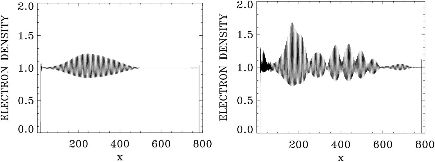
We present in Figure 9 the plots of the electron density at t = 533.3 and 800. Figure 10 presents the plots of the longitudinal electric field at t = 533.3 and 800. We now study the wavenumber spectra at a later time at t = 800. Figure 11 presents the frequency spectra for the signal recorded at x = 200, in the time interval t = (233,671). The frequency spectrum of E ⁺ shows the dominant frequencies presented in Figure 8, with the pump frequency appearing at ω_0P = 3.205, which is essentially the frequency 3.2 at which the pump is injected as we mentioned above. The wavenumber spectra response in the domain x = (100,537) are presented in Figure 12 at t = 800, slightly different from what we present in Figure 7. The wavenumber for E ⁺ in Figure 12 corresponding to the frequency ω_0P = 3.205 is k _0P = 3.061, in agreement with the value of 3.061 which can be calculated from Eq. (7) for ω_0P = 3.2 for a LCP. The forward re-scattered mode at 1.20 in Figure 11, which results from the forward re-scattering of the mode at the frequency 2.199 according to the selection rule 2.199 = ω_0F + 1.00, from which ω_0F = 1.199, as discussed in Figure 8 in the spectrum of E ⁺, is now more developed in Figure 11. The wavenumber for E ⁺ in Figure 12 corresponding to frequency ω_s = 1.2 is at k = 0.891, very close with the value of 0.8568, which can be calculated from Eq. (7) for ω_s = 1.2 for a LCP. The peaks in Figure 11 are the same frequencies as in Figure 8, although more developed, and we note in Figure 11 the important harmonic response for the plasma frequency in the spectrum of the longitudinal electric field. The wavenumbers response to these frequencies in Figure 12 shows the spectra, which are broad around the peaks, in contrast to what we see in Figure 7. In the present nonlinear stage, this points to a coupling with a RCP wave, which results in the broadening of the peaks in Figure 12. At the frequency 3.2 in Figure 11, Eq. (7) gives a wavenumber response of 3.061 for the LCP wave, and 3.01 for the RCP wave, well within the broad spectrum we see in Figure 12 around 3.061. Similarly at the frequency of 2.2 in Figure 11, Eq. (7) gives the wavenumber value of 2.006 for the LCP mode, and 1.90 for the RCP mode, within the broad peak we see around (1.983,2.04) in Figure 12. In addition to the scattering previously discussed in Figures 7 and 8 for the LCP modes, we have now couplings with the RCP modes, which explain the broadening we see in the wavenumber spectra in Figure 12. The frequency of the anti-Stokes resonance at 4.197 in Figure 11 leads from Eq. (7) to a wavenumber response at 4.09 for the LCP wave and 4.06 for the RCP wave. This RCP wave at wavenumber 4.06 can couple to the RCP wave at 3.01 to give the plasma response at the wavenumber 4.06–3.01 = 1.05, well within the broad peak we see in Figure 12 for the plasma response of the electric field around (1.035,1.135). Similarly the RCP wave at the wavenumber of 3.01 can couple with the RCP wave at the wavenumber 1.9 to give the plasma response in the electric field spectrum at the wavenumber 3.01–1.9 = 1.11, well within the broad peak around (1.035,1.135) we see in Figure 12 for the longitudinal electric field. So the broad peaks for the wavenumber harmonics in the spectrum of the longitudinal electric field in Figure 12 result from the coupling of LCP and RCP waves excited due to the high amplitude pump E ⁺. Finally, we observe in the spectrum of E ⁻ in Figures 11 and 12 peaks at the same frequencies and wavenumbers, but at a much lower level compared with E ⁺, due to the coupling in the nonlinear plasma medium as explained before. However, there is no backward scattered wave excited by the laser pump.

Fig. 9. The electron density at t = 533.3 (left frame) and t = 800 (right frame).

Fig. 10. The longitudinal electric field at t = 533.3 (left frame) and t = 800 (right frame).

Fig. 11. Temporal Fourier transform, calculated in the time interval t = (233,671), for the forward wave E ⁺, the backward wave E⁻, and the longitudinal electric field E _x, taken at the position x = 200.

Fig. 12. Spatial Fourier transform in the domain x = (100,537) of the forward wave E ⁺, the backward wave E⁻, and the longitudinal electric field E _x, at t = 800.

Finally, we present in Figure 13 the phase-space contour plots for the electron distribution function at t = 800, from x = 240 to 480. Between x = 400 and 440 we note the presence of about seven peaks, which leads to a wavelength of about 40/7 or 5.7. We get a close result if we consider the dominant wavenumber of the longitudinal electric field in Figure 12 at the average peak of 1.1, which leads to a wavelength ≈ 2π/1.1 = 5.7.

Fig. 13. Phase-space contour plots of the electron distribution function at different position in space at t = 800.

4. THE CASE OF THE BACKWARD RAMAN AMPLIFICATION OF A SEED PULSE

We consider a plasma where the electron cyclotron frequency is Ω_ce = 1.4, and the laser pump frequency is ω_0P = 3.2. From Eq. (7), the corresponding wavenumber for a LCP wave is 3.089, and for a RCP wave the corresponding wavenumber is 2.909. For the seed pulse, we take the frequency ω_0S = 2.17, which is the frequency we used in Section 3.1, and which from Eq. (7) corresponds to a wavenumber 2.025 for the LCP wave and 1.376 for the RCP wave.

The length of the system is L = 600. There is a uniform plasma slab of length L _p = 572.5, and a vacuum region of length L _vac = 12.5 on both sides of the slab, and a transition from vacuum to the plasma at the plasma edge of length L _edge = 15 on both sides, for a total length of 600. N = 120 000 grid points are used in space, and in our normalized units Δx = Δt = 0.005. The extrema of momentum for the electrons are ± 0.5, and with 1000 grid points in velocity space, we have a grid size of Δυ = 10⁻³. Ions were allowed to move in order to fix the small sheath at the edge of the plasma, but have otherwise no effect on the results. The units of time ${\rm \omega} _{{\rm pe}}^{ - 1} $ and space c/ω_pe we use can be easily translated into units of ${\rm \omega} _{0{\rm P}}^{ - 1} $ and c/ω_0P by dividing them by the factor, ω_0P/ω_pe = 3.2.

For the case considered for the problem of the Raman amplification of a seed pulse, we have a forward-propagating circularly polarized laser beam entering the system at the left boundary (x = 0) at the t = 0, and the forward-propagating fields of the circularly polarized constant amplitude pump are given at x = 0 by E ⁺ = 2E _0P cos (ω_0Pt) and F ⁻ = 2E _0P sin (ω_0Pt), E ⁺ and F ⁻ are defined in Eq. (5). We have in our normalized units E _0P = ω_0Pa _0P. The pump precursor reaches the right boundary x = 600 at t = 600, since in our normalized units x = t. The seed pulse is injected at the right boundary x = 600 in the backward direction just before the arrival of the pump, in the time interval 540 < t < 600, with E ⁻ = 2E _0SP _r(t) cos(ω_0S(t − 540)) and F ⁺ = −2E _0SP _r(t) sin(ω_0S(t − 540)), with E _0S = ω_0Sa _0S. We take the amplitude of the vector potential of the pump and the seed to be a _0P = a _0S = 0.04. The initial distribution functions for electrons and ions are Maxwellian with temperatures T _e = 0.35 keV for the electrons and T _i = 0.1 keV for the ions. The shape factor P _r(t) for the injected seed pulse has a Gaussian time dependence:

(8)$${P_{\rm r}}(t) = \exp {( - 0.5(t - 570)/{t_{\rm p}})^2};\,\,540 \lt t \lt 600;\,\,{t_{\rm p}} = 10.$$

The backward-propagating seed pulse behaves as a Gaussian pulse in time for 540 < t < 600, which reaches its peak at t = 570, and has completely penetrated the plasma at t = 600, that is, at the time the pump precursor reaches the right boundary.

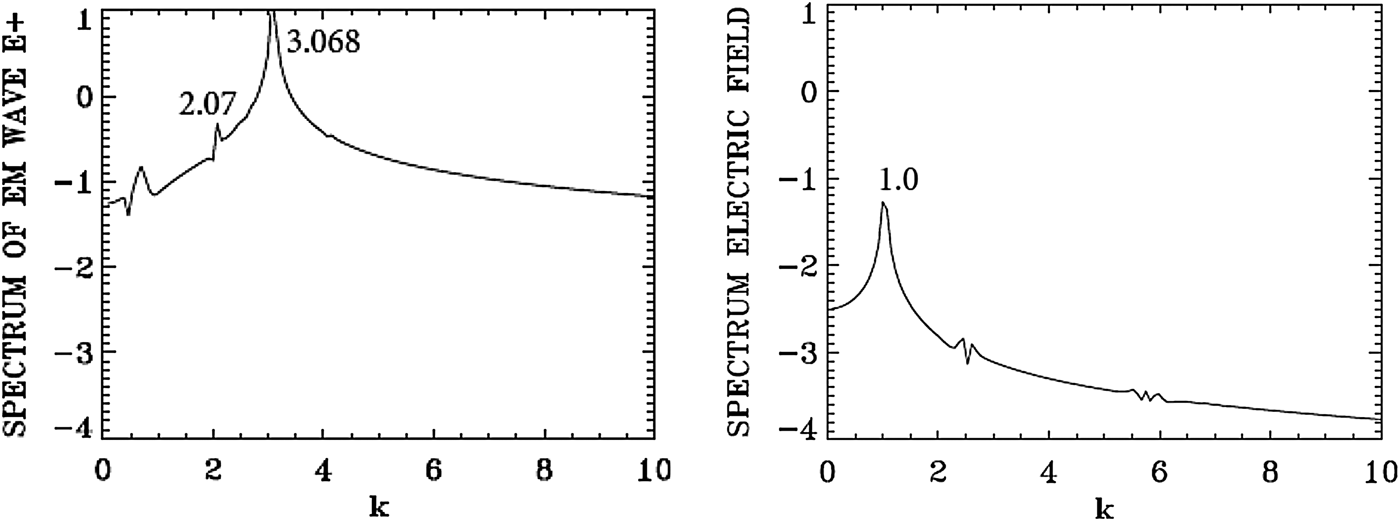
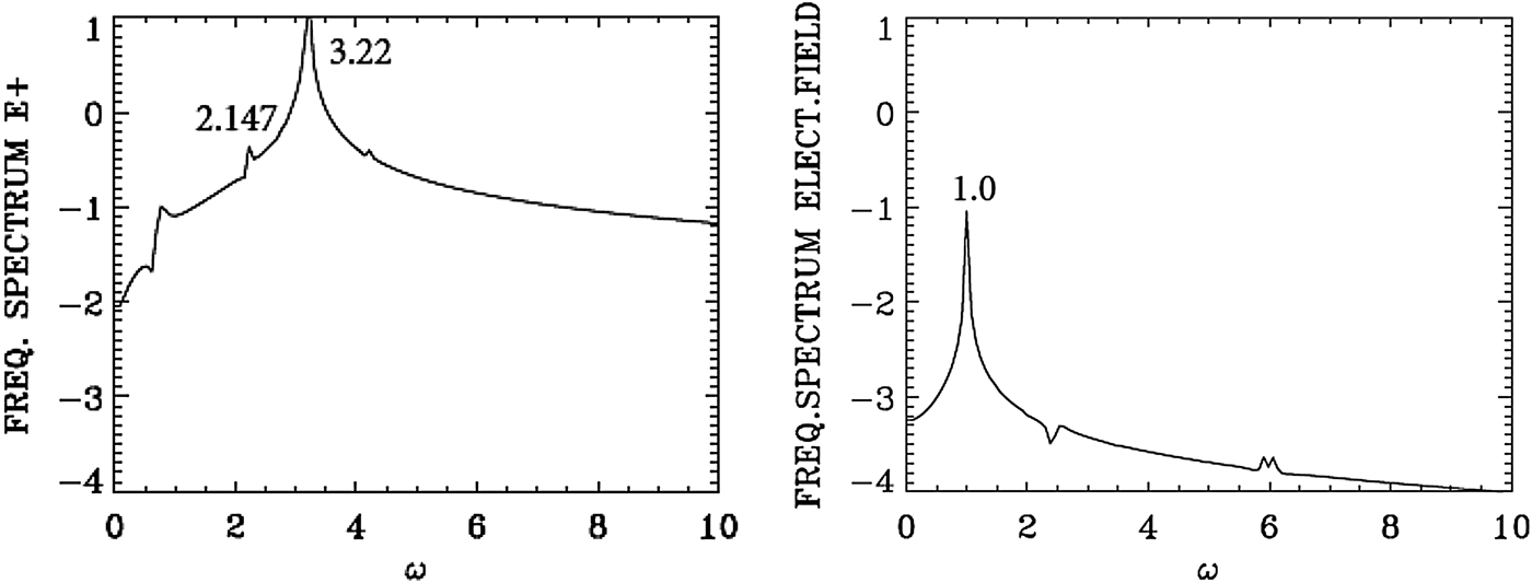
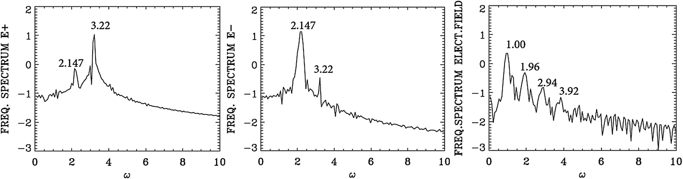
We present in Figure 14 the wavenumber spectra in the domain x = (450, 532) at t = 600, before the arrival of the injected backward seed pulse in this domain, which at t = 600 has penetrated to reach the point x = 540, according to the discussion of the previous paragraph. The spectrum for the pump E ⁺ shows a dominant peak at k _0P = 3.068, very close to the value of 3.089 calculated from the dispersion relation in Eq. (7) for the LCP wavenumber response to the injected pump at ω_0P = 3.2. It shows also a small forward scattered wave at 2.07, satisfying k _0P = 2.07 + k _e, from which we have for the plasma wave k _e = 3.068 − 2.07 = 0.998, which is essentially the value k _e ≈ 1 we see in Figure 14. We see indeed a low intensity and large peak in Figure 14 around the value of 1.0 in the spectrum of the longitudinal electric field. Due to the lower amplitude level of the laser pump (a _0P = 0.04) in the present calculation, the level of the excited forward scattered wave remained very low. As discussed in the previous section, the spectrum of E ⁻ shows essentially the same peaks as for E ⁺ due to the coupling in the nonlinear plasma medium, but remained much lower than E ⁺. No backward scattered wave developed.

Fig. 14. Spatial Fourier transform of the forward wave E ⁺ and the electric field E _x in the domain x = (450,532) at t = 600.

We present in Figure 15 the frequency spectrum corresponding to the results presented in Figure 14. The temporal Fourier transform of E ⁺ is taken at the position x = 450 in the time interval t = (545,632), before the arrival of the backward seed pulse injected at the right of the domain. The peak frequency of the injected pump E ⁺ at the frequency 3.2 is appearing in Figure 15 at 3.22. The frequency of the forward scattered mode appears at 2.147 [the corresponding wavenumber calculated from the dispersion relation in Eq. (7) gives for the LCP wave the value of 2.00, close to the value of 2.07 calculated in Figure 14]. From the plasma wave dispersion relation ${\rm \omega} _{\rm e}^2 = 1 + 3k_{\rm e}^2 ({\rm \upsilon} _{\rm t}^2 /{c^2})$, and T _e is 0.35 keV in the present calculation, we get for k _e = 1.0 the plasma frequency ω_e = 1.00, which is the result we see in Figure 15 in the frequency spectrum of the longitudinal electric field.

Fig. 15. Temporal Fourier transform of the forward wave E ⁺ (full curve) and the electric field E _x for time interval t = (545,632) at the position x = 450.

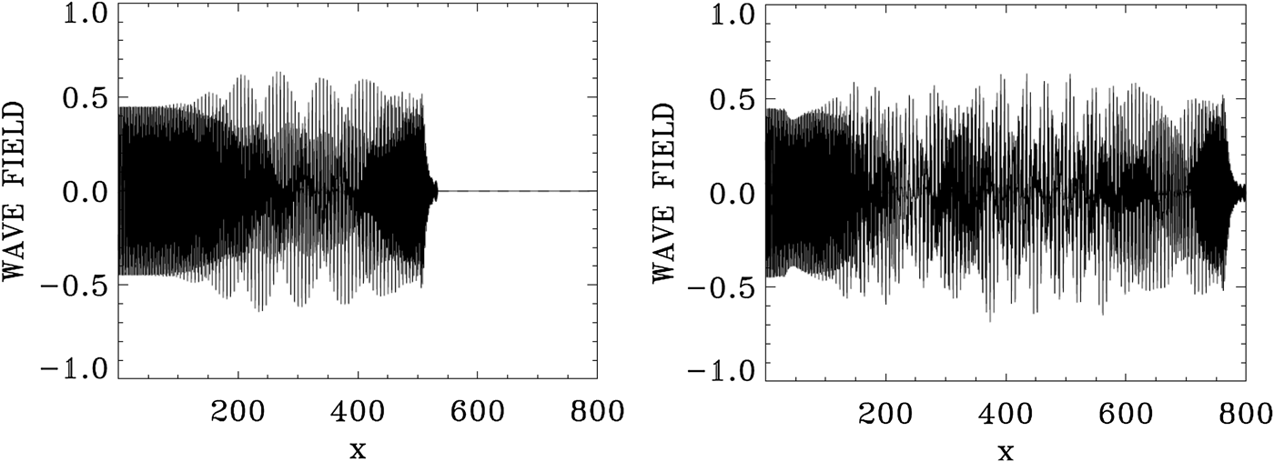
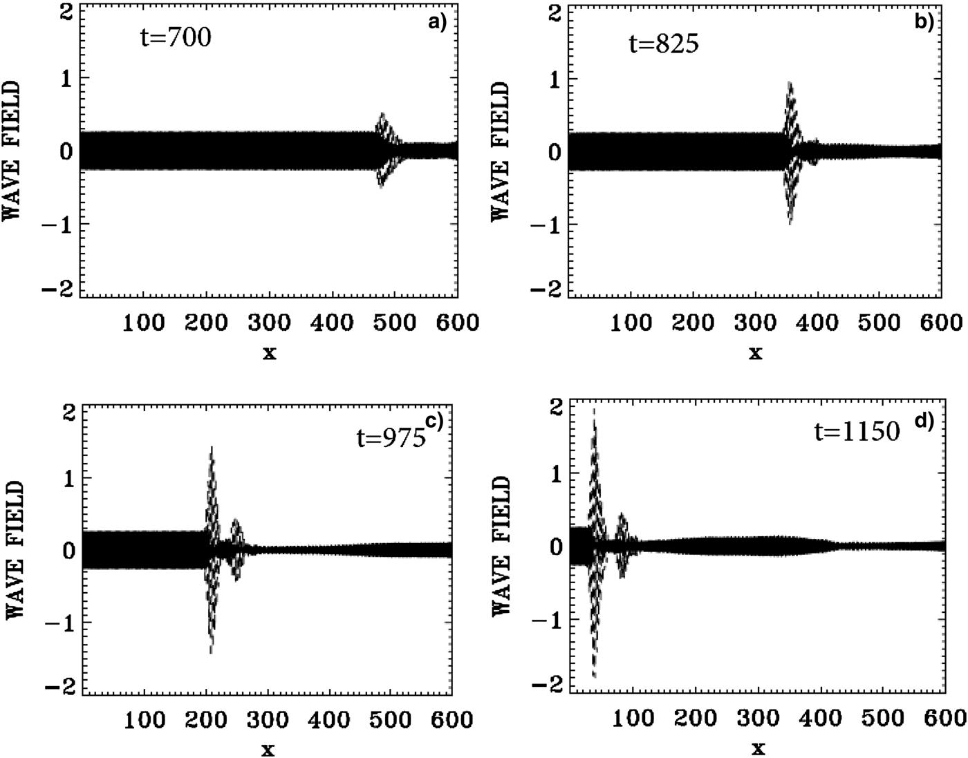
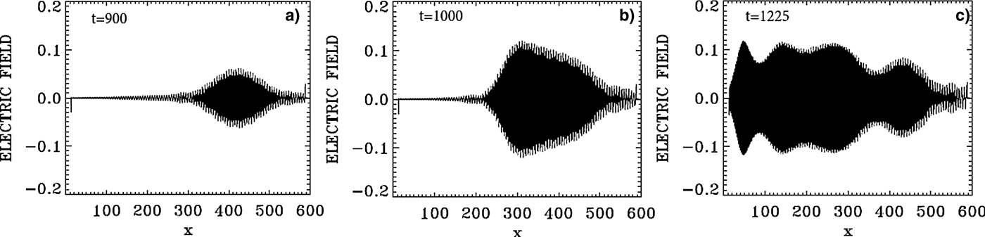
The evolution of the incident pump wave E ⁺ (full curve) and the backward seed pulse E ⁻ (dashed curve) are shown in Figure 16 at: (a) t = 700, (b) t = 825, (c) t = 975, (d) t = 1150. We note the growth and compression of the seed pulse E ⁻, propagating toward the left, together with an increase in the waveform steepness. The modulation we see behind the front pulse of the growing seed are due to the fact that when the pump depletes, the seed pulse will act as a source for the pump, which results in a modulation behind the growing seed. The constant amplitude full-curve at the left in Figure 16 is for the injected constant amplitude pump. At t = 1150, the backward seed pulse is about 25 times its original amplitude, and about eight times higher than the pump amplitude.

Fig. 16. The evolution of the incident pump wave E ⁺ (full curve) and the backward seed pulse E⁻ (dashed curve) at: (a) t = 700, (b) t = 825, (c) t = 975, (d) t = 1150.

In what we present next, we will follow at different time the growth of the backward propagating seed pulse in different sections of the domain. In the results we analyze, we will show the dominance of a backward Raman scattering in the process of the amplification of the backward seed pulse all over the domain.

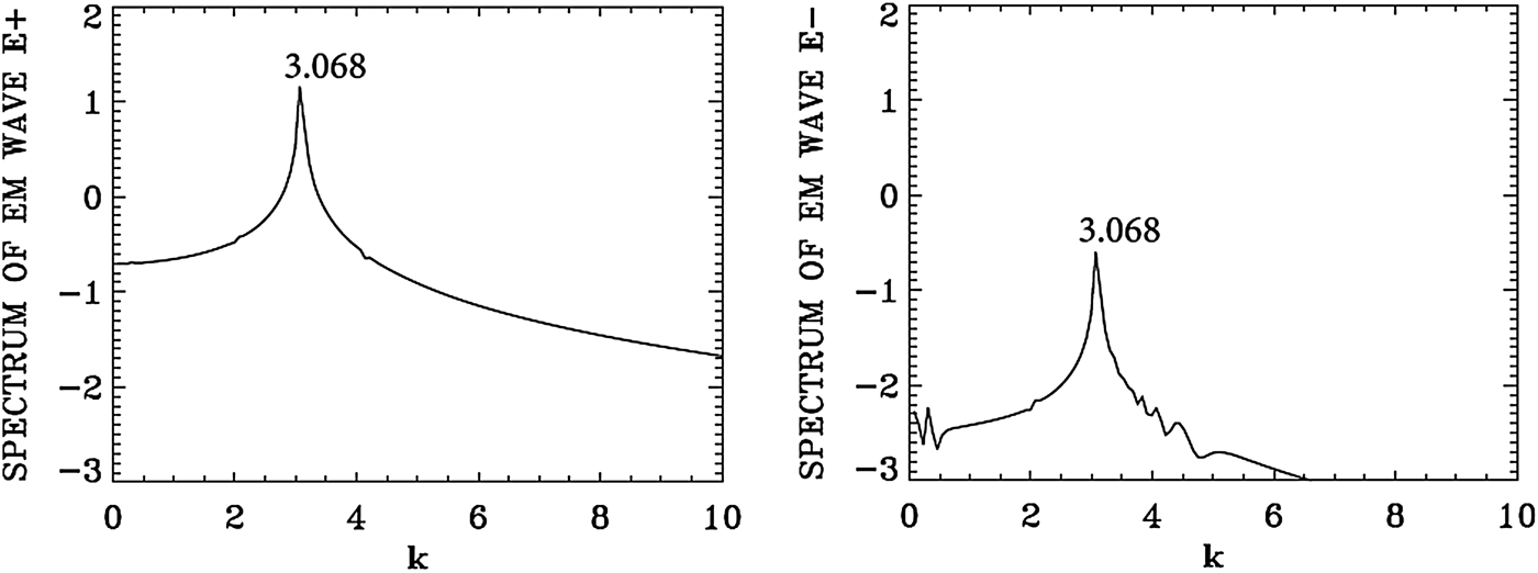
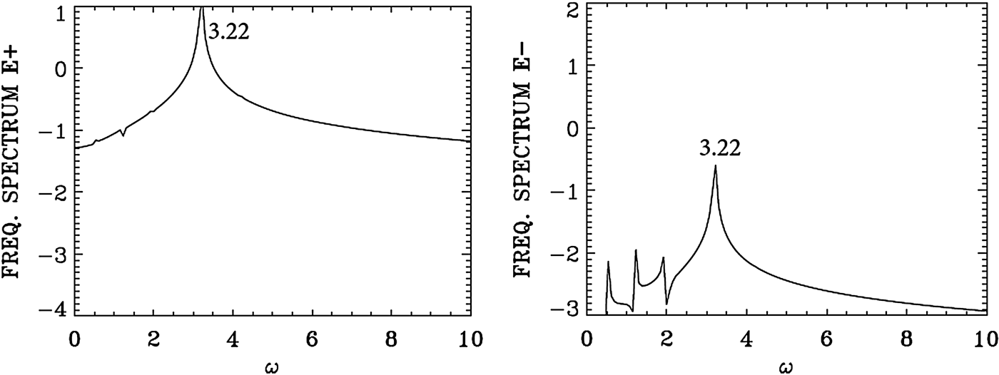
We present in Figure 17 the wavenumber spectra at the time t = 720 in the same domain x = (450, 532) as in Figure 14, that is, after the arrival in this domain of the seed pulse injected with ω_0S = 2.17 from the right boundary. In Figure 17, we see a dominant wavenumber for the backward wave E ⁻ at k _0S = 2.07. The corresponding frequency spectra are given in Figure 18, calculated by taking a temporal Fourier transform in the time interval t = (685,767), by monitoring the signal at the position x = 450. We see for the backward wave E ⁻ a dominant broad peak at ω_0S = 2.147, very close to the injected value of 2.17. The corresponding wavenumber to the frequency 2.147 calculated from the dispersion relation in Eq. (7) is 2.00, very close to the value of 2.07 calculated for the wavenumber of E ⁻ in Figure 17. We see the trace of the backward mode at 2.07 in the spectrum of E ⁻ appearing in the spectrum of E ⁺ in Figure 17 at 2.07, together with the wavenumber of the forward propagating pump wave E ⁺ at k _0P = 3.068. The corresponding frequency of the forward pump E ⁺ in Figure 18 is ω_0P = 3.22.

Fig. 17. Spatial Fourier transform of the incident pump wave E ⁺, the backward wave E⁻, and the longitudinal electric field E _x, calculated in the domain x = (450,532) at time t = 720.

Fig. 18. Temporal Fourier transform of the incident pump wave E ⁺, the backward wave E ⁻, monitored at the position x = 450, in the time interval t = (685,767).

The plasma wavenumber k _e and frequency ω_e must satisfy the selection rule for the momentum and energy conservation relations for the backward wave k _0P = −k _0S + k _e, and ω_0P = ω_0S + ω_e. We get ω_e = 1.07, and k _e = 5.138, which is the peak value we see in Figure 17 for the spectrum of the electric field, which shows the value of 5.138 and its harmonics. From the plasma wave dispersion relation ${\rm \omega} _{\rm e}^2 = 1 + 3k_{\rm e}^2 ({\rm \upsilon} _{\rm t}^2 /{c^2})$, we get for the plasma frequency ω_e = 1.0267 for T _e = 0.35 keV, with the value k _e = 5.138, close to the value of 1.07 calculated from the selection rule. We note a broad spectrum around 1.0 in Figure 18 for the plasma wave frequency. Note also the harmonic structure associated with the plasma frequency.

We note also in Figure 17 the plasma wave at 1.07 and the pump wave at the wavenumber 3.068 will combine to excite the anti-Stokes at 4.138, close to the value of 4.141 we see in the spectrum of E ⁺ in Figure 17. The corresponding frequencies in Figure 18 of 1.00 and 3.22, excite the anti-Stokes at the frequency 4.22 (a very small bump, not marked in the frequency spectrum of E ⁺ in Figure 18). The corresponding wavenumber to the frequency 4.22 calculated from Eq. (7) for the LCP wave is 4.12, very close to the value of 4.141 in Figure 17.

In addition to the backward scattering k _0P = −k _0S + k _e, ω_0P = ω_0S + ω_e, which is exciting the backscattered mode in E ⁻ at ω_0S = 2.147 (see Figure 18) and k _0S = 2.07 (see Figure 17) we have a weak forward scattered mode at the same wavenumber and frequency k _0P = k _0S + k _e, from which k _e = 3.068 − 2.07 = 0.997 (close to the value of 1.07 we see in Figure 17), and ω_e = ω_0P − ω_0S = 3.22 − 2.147 = 1.073 (see the broad peak around 1.0 in Figure 18).

We follow again the backward Raman scattering amplification in another domain closer to the left boundary. We present in Figure 19 the wavenumber spectra close to the left boundary, in the domain x = (30, 112) at t = 900, before the arrival of the injected backward seed pulse which, at t = 900, has only reached around the point x = 240. The spectrum for the pump E ⁺ shows a dominant peak of the forward pump at k _0P = 3.068. As we mentioned above, E ⁺ and E ⁻ are strictly decoupled in vacuum, a very small backward wave E ⁻ at the same wavenumber 3.068 results from the coupling with E ⁺ in the nonlinear plasma medium; otherwise no other backward or forward scattered wave is present, before the arrival of the backward seed pulse.

Fig. 19. Spatial Fourier transform of the incident pump wave E ⁺, the backward wave E⁻, in the domain x = (30,112) at t = 900.

We present in Figure 20 the frequency spectrum corresponding to the results presented in Figure 19, calculated by monitoring the signal at the position x = 80, and making a temporal Fourier transform of the signal in the interval of time t = (500,582), before the arrival of the backward seed pulse. The peak frequency of the injected pump E ⁺ at 3.2 is appearing in Figure 20 at 3.22. So only the forward pump is present before the arrival of the backward signal. Again, as explained before, there is a small backward wave E ⁻ at the same frequency, which results from the coupling in the nonlinear plasma medium with E ⁺, but no other backward or forward scattered wave is present before the arrival of the counter-propagating backward seed pulse.

Fig. 20. Temporal Fourier spectrum of the incident pump wave E ⁺, the backward wave E⁻, monitored at the position x = 80, in the time interval t = (500,582).

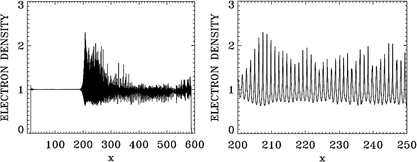
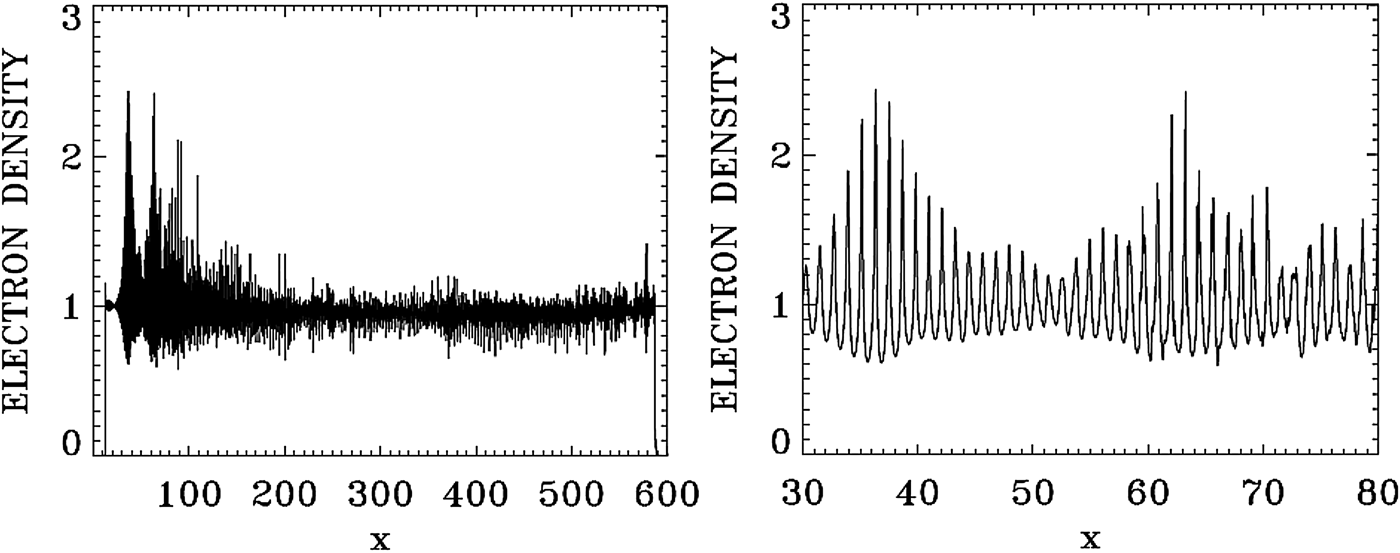
In Figure 21, we present a plot for the electron density profile at t = 975 (left frame). The right frame in Figure 21 zoom on the front edge of the profile, in x ∈ (200, 250), which shows clearly the regular oscillations of the dominant growing mode with wavenumber k _e = 5.138, and wavelength λ_e = 2π/k _e = 1.22. Figure 22 presents a plot for the electron density profile at t = 1150 (left frame). The right frame in Figure 22 zoom on the front edge of the profile, in x ∈ (30, 80). Figure 24 below shows the dominant mode at that time has shifted to k _e = 5.292, with the corresponding wavelength λ_e = 2π/k _e = 1.18. So the growth of the pulse is continuing, as verified from Figure 16, as long as the front part of the pulse is maintaining its coherent structure. In the domain besides the front part, the fusion of the vortices in phase-space due to the competing modes creates a chaotic structure (see Figure 25 below).

Fig. 21. Plot of the electron density profile at t = 975.

Fig. 22. Plot of the electron density profile at t = 1150.

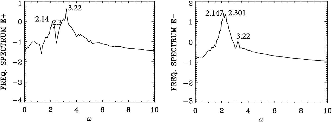
We present in Figure 23 the frequency spectrum at the front part of the growing pulse, by monitoring the signal at the position x = 80, calculated by taking the temporal Fourier transform in time in the interval t = (1100,1192) after the arrival of the backward signal. Figure 16 shows the steepening of the profile. We see again the peak frequency of the forward pump E ⁺ at 3.2 is appearing in Figure 23 at 3.22. The backward wave E ⁻ shows now dominant frequencies over a broad peak extending from 2.147 to 2.301 (the backward seed was injected at the right boundary at the frequency 2.17). This same frequencies (2.147, 2.301) are appearing in the spectrum of E ⁺ due the coupling in the nonlinear plasma medium. The backward seed pulse arrived at the position x = 80 at about t = 1120. So the frequency spectrum of the electric field is still at its early development and did not have the time to develop a harmonic structure as in Figure 18. It shows a broad peak around 1.0.

Fig. 23. Temporal Fourier transform for the incident pump wave E ⁺, and the backward wave E⁻, monitored at the position x = 80, in the time interval t = (1100,1192).

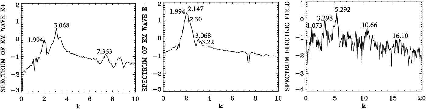
We present in Figure 24 the wavenumber spectra at the front part of the growing pulse, by taking the spatial Fourier transform in the domain x = (30, 112) at t = 1150. Slightly broader peaks are appearing in the wavenumber spectrum for E ⁻ at 1.994 and 2.147 corresponds to the frequencies for E ⁻ at 2.147 and 2.30, respectively in Figure 23 [from Eq. (7), for a LCP wave, for a frequency 2.147 corresponds a wavenumber 2.00, and for a frequency 2.30 corresponds a wavenumber 2.16, very close to the peak values of 1.994 and 2.147 we see in Figure 24 for E ⁻]. For E ⁺, we have in Figure 24 the wavenumber 3.068, corresponding to the frequency 3.22 in Figure 23 (the injected pump frequency for E ⁺ is 3.2 as previously mentioned).

Fig. 24. Spatial Fourier transform of the forward wave E ⁺, the backward wave E ⁻ and the longitudinal electric field E _x, in the domain x = (30,112) at t = 1150.

The plasma wavenumber k _e and ω_e must satisfy the selection rule for the momentum and energy conservation relations for the backward wave k _0P = −k _0S + k _e, and ω_0P = ω_0S + ω_e. With k _0P = 3.068 and k _0S = 2.147 we get k _e = 5.215, which is very close to the value we see in Figure 24 for the spectrum of the electric field E _x which shows the peak at 5.292 and its harmonics. From the plasma wave dispersion relation ${\rm \omega} _{\rm e}^2 = 1 + 3k_{\rm e}^2 ({\rm \upsilon} _{\rm t}^2 /{c^2})$, we get for the plasma frequency ω_e = 1.028 for T _e = 0.35 keV, with the value k _e = 5.292, close to the value of 1.07 calculated from the selection rule. Note in the spectrum of E ⁺ the presence of a weak forward coupling with the mode at the wavenumber 1.994, following the selection rule 3.068 = 1.994 + 1.074 (see the plasma mode at 1.073 in Figure 24).

The left frame in Figure 25 shows the contour plot of the electron distribution function at t = 1150 at the front edge in x ∈ (30, 60). It shows in the left frame the regular oscillations of the dominant growing mode of the steep pulse with the wavelength λ_e = 2π/k _e = 1.18, corresponding to dominant value of k _e = 5.292 we see in Figure 24. In the right frame, the phase-space contour plot of the distribution function at t = 1150 in x ∈ (60, 90) shows a tendency to become more chaotic, as it is also apparent in the density plot of Figure 22.

Fig. 25. Contour plot of the electron distribution function at t = 1150, for 30 < x < 60 and 60 < x < 90.

In the results we have presented in this section, we have followed at different positions and time the growth of the backward propagating seed-pulse in different section of the domain. In the results we analyzed we have shown the dominance of a backward SRS in the process of the amplification of the backward seed-pulse all over the domain. We have also shown that before the arrival of the counter-propagating backward seed pulse, no backward SRS was present in the domain.

5. THE CASE OF THE BRILLOUIN AMPLIFICATION OF A SEED PULSE

We consider a plasma such that the electron cyclotron frequency is Ω_ce = 1.4, and the laser pump frequency is ω_0P = 2.17. From Eq. (7), the corresponding wavenumber for a LCP wave is 2.025, and for a RCP wave the corresponding wavenumber is 1.376. The SBS produces a very small frequency downshift in the scattered wave ω_0P = ω_0S + ω_ion. We neglect this small downshift ω_ion ≪ 1 and set the seed frequency ω_0S ≈ ω_0P = 2.17 for a LCP wave (and hence k _0S ≈ k _0P = 2.025). The SBS is backward-propagating, so the selection rule is k _0P = −k _0S + k _ion, and hence the wavenumber of the ion wave k _ion ≈ 2k _0P = 4.05. We also take for the vector potentials of the waves a _0S = a _0P = 0.04, and the parameters of the counter-propagating seed pulse injected at the right boundary are the same as in Eq. (8). We have the same length L = 600 as in the previous section.

For the electron distribution function, the extrema of momentum for the electrons are ± 0.5, and with 1000 grid points in velocity space, we have a grid size of Δυ = 10⁻³. For the ions the extrema of momentum are ± 1.46 × 10⁻³, and with 500 grid points in velocity space, we have a grid size of Δυ = 5.85 × 10⁻⁶. The initial distribution functions are Maxwellian with temperatures T _e = 0.3 keV for the electrons and T _i = 0.02 keV for the ions. The parameters of the plasma slab are the same as in Section 4, with Δx = Δt = 0.005.

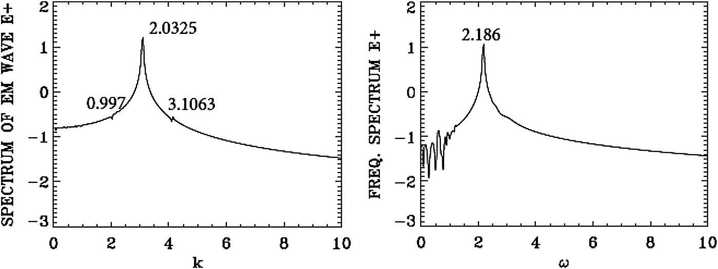
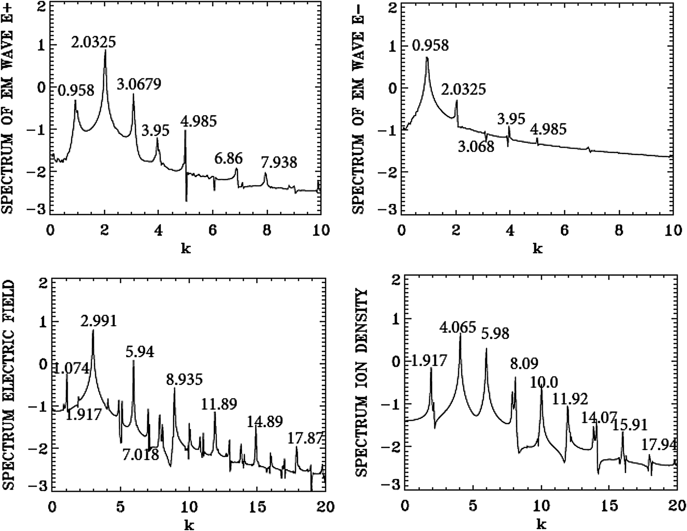
We present in Figure 26 the wavenumber spectra in the domain x = (30, 224) at t = 600, before the arrival of the injected backward seed-pulse, which at t = 600 has only penetrated to the point x = 540, according to the discussion for Eq. (8) of the previous section. The spectrum for the pump E ⁺ shows a dominant peak at k _0P = 2.0325, very close to the value of 2.025 calculated as mentioned above from Eq. (7) for the LCP wavenumber response to the injected pump at ω_0P = 2.17. Figure 26 shows also for the frequency spectrum of the pump (in the right frame) the value of 2.186, very close to the injected value of 2.17. The frequency spectrum is calculated by taking the temporal Fourier transform of the signal, recorded at the position x = 90 in t = (100,294). The forward pump is the only wave present, the backward seed pulse did not reach the domain x = (30, 224) at t = 600. So the spectrum of E ⁻ is essentially the same as in Figure 26, due to the coupling of E ⁻ and E ⁺ in the nonlinear plasma medium, with E ⁻ much smaller than E ⁺ as previously mentioned. There is no backward scattered mode. Figure 26 shows also a small forward excited wave at 0.997, satisfying k _0P = 0.997 + k _e1, from which we have for the plasma wave of the longitudinal electric field k _e1 = 2.0325 − 0.997 = 1.0355, and the corresponding frequency calculated from the plasma wave dispersion relation 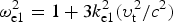${\rm \omega} _{{\rm e}1}^2 = 1 + 3k_{{\rm e}1}^2 ({\rm \upsilon} _{\rm t}^2 /{c^2})$, from which ω_e1 = 1.00. The spatial spectrum of the longitudinal electric field shows indeed a small peak at 1.0738, and the temporal spectrum shows indeed a peak at 1.00. This will be discussed in more details in Figures 28 and 29. In Figure 26, we have also a very small trace of the anti-Stokes at 3.1063, resonating with a plasma wave at the wavenumber 1.0738 = 3.1063–2.0325, with a corresponding plasma frequency of 1.00. The frequency resonance is 2.186 + 1.00 = 3.186. The wavenumber for the anti-Stokes calculated from Eq. (7) for the frequency 3.186 is 3.075, close to the value of 3.1063 in Figure 26. There is no backward seed pulse injected at the right boundary which has yet arrived in the domain x = (30, 224).

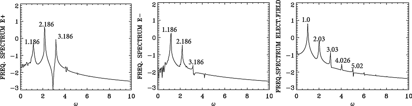
Fig. 26. Spatial Fourier spectrum of the incident pump wave E ⁺ in the domain x = (30,224) at t = 600 (right frame), and temporal Fourier spectrum of the incident pump wave E ⁺ in the time interval t = (100,294) at the position x = 90 (left frame).

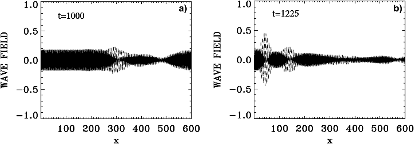
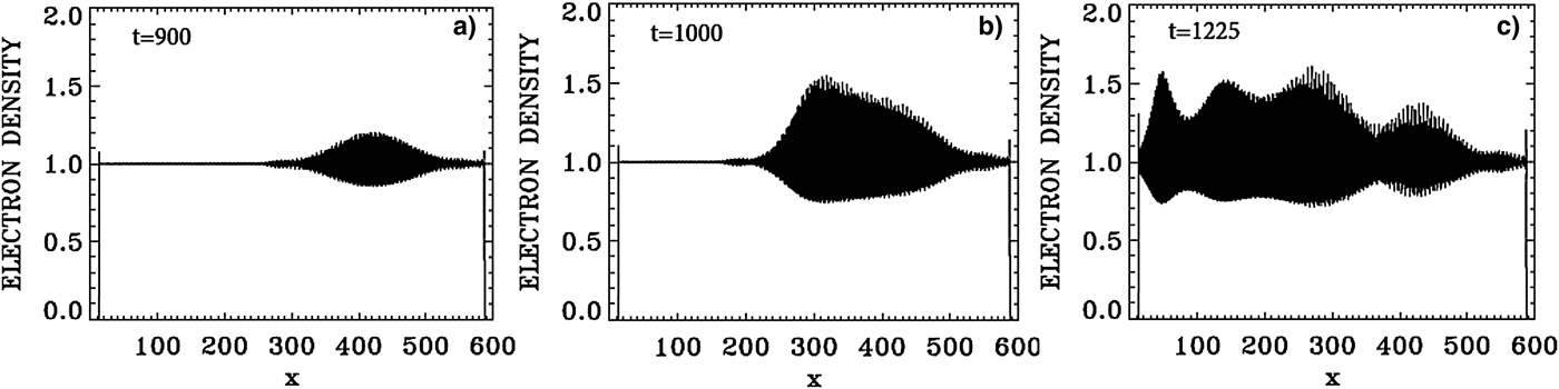
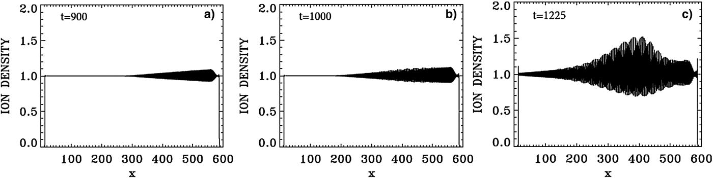
The evolution of the incident pump wave E ⁺ (full curve) and the backward seed pulse E ⁻ (dashed curve) are shown in Figure 27 at: (a) t = 1000, (b) t = 1225. We note the growth and contraction of the seed pulse, propagating toward the left. The modulation we see behind the front pulse of the growing seed are due to the fact that when the pump depletes, the seed pulse will act as a source for the pump, which results in a modulation behind the growing seed. The constant amplitude full-curve at the left in Figure 27(a) is for the constant amplitude incident pump. The original amplitude of the seed was equal the amplitude of the pump. At the end at t = 1225 in Figure 27, the backward seed pulse is about two times of its original amplitude.

Fig. 27. The evolution of the incident pump wave E ⁺ (full curve) and the backward seed pulse E⁻ (dashed curve) at: (a) t = 1000, (b) t = 1125.

In Figure 28, the wavenumber spectra associated with the forward wave E ⁺, the backward wave E ⁻, the longitudinal electric field E _x, and the ion density, are calculated by Fourier transform of the corresponding signal in the domain x = (200,394), which has been reached by the backward seed pulse at t = 1000. The spectrum of the electron density is essentially the same as the one presented for the longitudinal electric field in Figure 28. The spectrum of E ⁺ in Figure 28 shows the peak of the forward pump at 2.0325, as we mentioned in Figure 26, and the same mode appearing as a backward mode in the spectrum of E ⁻ in Figure 28. The presence of these two modes will result in the appearance of a backward Brillouin scattering as discussed above, with an ion wavenumber k _ion ≈ 2k _0P = 4.065, which is indeed appearing the spectrum of the ion density in Figure 28. We also note in the spectrum of E ⁺ in Figures 26 and 28 the presence of the forward scattered mode at 0.958, with the plasma mode at 1.074 apparent in the spectrum of the electric field E _x in Figure 28, such that 2.032 = 0.958 + 1.074. The corresponding frequencies we see in Figure 29, calculated by taking the temporal Fourier transform of the signal recorded at x = 300, between t = (1000,1194), give a frequency ω_0P = 2.186 for the pump and ω_0S = 1.186 for the forward scattered mode. The corresponding wavenumbers calculated from Eq. (7) are respectively 2.042 (very close to the value of 2.032 in Figure 28) and 0.973 (very close to the value of 0.958 in Figure 28). This gives a plasma wavenumber 1.069 = 2.042–0.973, close to the value of 1.074 calculated in Figure 28 in the spectrum of E _x. The corresponding plasma frequency is calculated from the plasma wave dispersion relation ${\rm \omega} _{\rm e}^2 = 1 + 3k_{\rm e}^2 ({\rm \upsilon} _{\rm t}^2 /{c^2})$. We get for k _e = 1.069 the plasma frequency ω_e = 1.00, in good agreement with the value in Figure 29 in the spectrum of E _x, satisfying the frequency selection rule 2.186–1.186 = 1.00.

Fig. 28. Spatial Fourier transform of the forward pump wave E ⁺, the backward seed pulse E⁻, the longitudinal electric field E _x and the ion density in the domain x = (200,394) at t = 1000.

Fig. 29. Temporal Fourier transform of the signal recorded at x = 300, in the time interval t = (1000,1194), for the forward pump wave E ⁺, the backward wave E⁻, and the longitudinal electric field E _x.

We have also in the spectrum of E ⁻ a backward scattered mode at 0.985 in Figure 28, which is dominating the spectrum of E ⁻, such that k _0P = −k _0S + k _e, that is 2.0325 = −0.985 + 2.9905. We see indeed the mode at 2.991 in the spectrum of the electric field in Figure 28. The forward scattered mode at 0.985 in E ⁺ and the backward mode in E ⁻ at 0.985, will couple through Brillouin scattering to give another Brillouin scattered mode at k _ion ≈ 2 × 0.958 = 1.916, which appears at 1.917 in the spectrum of the ion density in Figure 28. So we have two Brillouin scattering events, one at k _ion ≈ 2k _0P = 4.065 through direct scattering from the pump E ⁺ and the backward seed pulse, and the second one through an intermediate step of forward and backward Raman scattering of the pump, which produced the modes at 0.958 in E ⁺ and − 0.958 in E ⁻, from which the ion mode wavenumber ≈ 2 × 0.958 = 1.916. Other resonances are also present. We can identify in the spectrum of E ⁺ the anti-Stokes at 3.0679 obtained by the coupling of the plasma mode at 1.074 and the pump E ⁺ at the wavenumber at 2.0325 such that 3.1065 = 2.0325 + 1.074, close to the value of 3.0679 we see in the wavenumber spectrum of E ⁺ in Figure 28. From Figure 29 the corresponding longitudinal plasma frequency is ω_e = 1.00, the corresponding frequency to the anti-Stokes mode is 3.186, which verifies the selection rule for the frequencies 3.186 = 2.186 + 1.00. The wavenumber for the anti-Stokes calculated from Eq. (7) for the frequency 3.186 is 3.075, close to the value of 3.0679 in Figure 28.

The modes in E ⁺ in Figure 28 at 2.035 and 3.95 will combine with the mode at 1.917 in the longitudinal electric field such that 3.95 = 2.0325 + 1.917, with the corresponding frequencies in Figure 29 satisfying the selection rule 3.18 + 1.01 = 4.19 (the unmarked small peak in Figure 29 in the spectrum of E ⁺).

The forward mode at 4.985 in E ⁺ and the backward mode at – 0.985 in E ⁻ in Figure 28 will couple to produce the mode in the longitudinal electric field 4.985 = – 0.985 +k _e, from which the plasma wavenumber k _e = 5.94, which appears in the spectrum of E _x in Figure 28. The ion mode at 5.98 will couple with the two ion modes at 4.065 and 1.915, 4.065 + 1.915 = 5.98, and the ion mode at ten couples with two ion modes 4.065 + 5.98 = 10.045, and with the two ion modes 8.09 + 1.917 = 10.007. The corresponding ion acoustic frequencies for these ion modes with the dispersion relation ω = kC _s, where C _s is the ion acoustic speed, will automatically satisfy the selection rules, because of the linear dependence of ω and k in the dispersion relation of the ion acoustic waves.

We note the harmonic structure associated with the plasma wavenumber of 2.991 in the wavenumber spectrum of the longitudinal electric field in Figure 28 at 5.94, 8.935, 11.89, 14.89, 17.87, and the harmonic structure with the plasma frequency in Figure 29. We also note the harmonic structure associated with the ion mode at the wavenumber 4.065 at 8.09, 11.92, 15.91, and the harmonic structure associated with the ion mode with the wavenumber 5.98 at 11.92 and 17.94 in Figure 28.

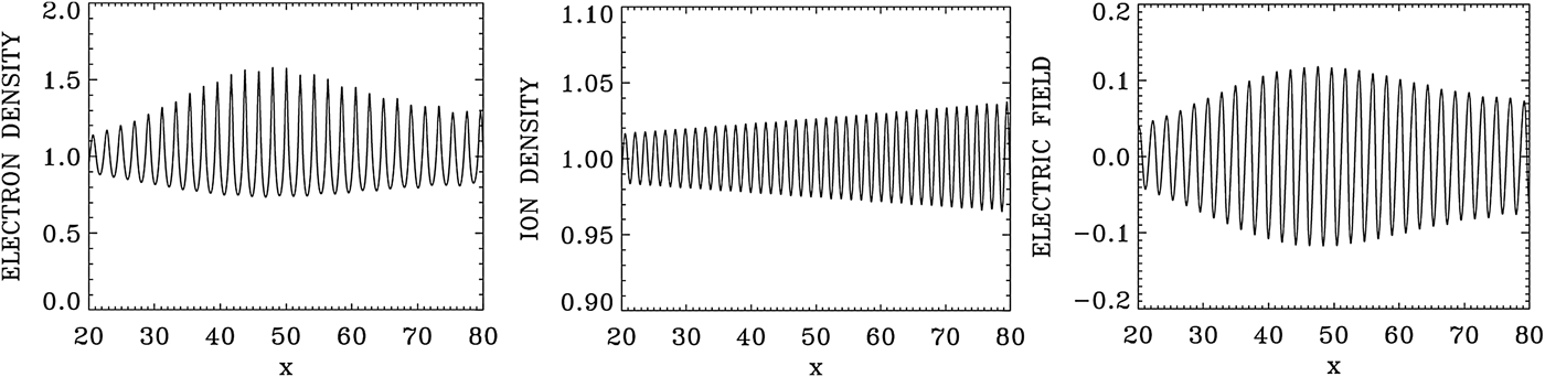
Figure 30 presents a plot for the electron density profiles at t = 900, 1000, and 1225. Similar plots are presented in Figure 31 for the ion density profiles, and in Figure 32 for the electric field profiles. In Figure 33, we zoom on the front edge of the profiles in x = (30, 80), which shows at t = 1225 the regular oscillations of the dominant growing mode with wavelength λ_e = 2π/2.99 = 2.1 for the electron density and the longitudinal electric field, and λ_i = 2π/4.065 = 1.54 for the ion density profile (Figs 33–35).

Fig. 30. Plot of the electron density profiles at: (a) t = 900, (b) t = 1000, (c) t = 1225.

Fig. 31. Plot of the ion density profiles at: (a) t = 900, (b) t = 1000, (c) t = 1225.

Fig. 32. Plot of the longitudinal electric field E _x at: (a) t = 900, (b) t = 1000, (c) t = 1225.

Fig. 33. Zoom on the front edge of the profiles in x = (30,80) at t = 1225.

Fig. 34. Phase-space contour plot of the electron distribution function at t = 1225, at different positions.

Fig. 35. Phase-space contour plot of the ion distribution function at t = 1225, at different positions.

In the results, we have presented in this section, two backward Brillouin scattering events are present. The first one results directly from the pump and the counter-propagating seed pulse, both injected at the same frequency ω_0S ≈ ω_0P = 2.17. The second backward Brillouin scattering event takes place via the intermediate step of two Raman scattering processes, which create the counter-propagating modes in E ⁺ and E ⁻ at the wavenumber 0.958, and a resulting SBS mode at the wavenumber 2 × 0.958 = 1.916, which we see in Figure 28 in the spectrum of the ion density.

6. THE CASE OF THE WAKEFIELD ACCELERATOR IN A MAGNETIZED PLASMA

A solution of this problem in an un-magnetized plasma using an Eulerian Vlasov code has been given by Shoucri (Reference Shoucri2008b). The application of an external magnetic field in the problem of wakefield acceleration has been suggested by Grulke et al. (Reference Grulke, Buttenschön and Fahrenkamp2015) to stabilize the plasma column. We consider a plasma such that the ratio of the electron cyclotron frequency to the electron plasma frequency Ω_ce = 0.1, and the ratio of the laser pump frequency to the electron plasma frequency ω_0P = 10 ≫ 1. We use N _x = 50 000 grid points in space for a total length of the plasma L = 50. The extrema of the electrons momentum are ± 20, with a number of grid points N _pe = 5000, and for the ions momentum extrema we have ± 1.25 × 10⁻⁴, with a number of grid points N _pi = 400. The electron and ion temperatures are T _e = 0.2 keV and T _i = 0.01 keV. The length of the vacuum region is 0.166 on each side, and the length of the transition region for the zero density to the flat density of 1 is 1.0 on each side of the slab, hence a total transition region of 1.166 on each side of the plasma slab. The system is initially neutral (n _e = n _i), with the density in the flat neutral part equal to 1 in our normalized units. We note the ions density remained equal to 1 in the flat central part, the ions however showing a modulation in the phase-space contour plots.

The forward propagating circularly polarized laser pulse is penetrating from the vacuum at the left boundary at x = 0, and propagate toward the right, and is written in our normalized units as:

(9)$${E^ +} = 2{E_0}\sin ({\rm \pi} {\rm \xi} /{L_x})\sin ({k_{0{\rm P}}}{\rm \xi} ),$$

(10)$${F^ -} = 2{E_0}\sin ({\rm \pi} {\rm \xi} /{L_x})cos({k_{0{\rm P}}}{\rm \xi} ),$$

for 1 < t < 2π + 1, and for −L _x < ξ <0, ξ = x − t, and E ₀ = 0 otherwise. The time delay 1 corresponds approximately to the length 1.166 of the vacuum and transition region as mentioned above. This allows the pulse to develop close to the edge of the flat part of the density profile. L _x is the length of the pulse envelope. In vacuum, we have for the EM wave k _0P = ω_0P. So in our normalized units the vacuum wavelength λ = 2π/k _0P = 0.628. We have ten oscillations for the EM wave in the length L _x = 2π of the pulse envelope. Note that the wavenumber inside the plasma can be calculated from Eq. (7), and for Ω_ce = 0.1 and ω_0P = 10 gives k _0P ≈ 9.95, close to the vacuum value of 10. We choose for the amplitude of the potential vector a _0P = 0.8, so that E ₀ = ω_0Pa _0P = 8. From Eqs. (9) and (10) the amplitude of E ⁺ and F ⁻ are equal to 2E ₀. Since the envelope is very slowly varying, we can write for the corresponding vector potential for 1 < t < 2π + 1:

(11)$${a_y} = - {a_{0{\rm P}}}\sin ({\rm \pi} {\rm \xi} /{L_x})cos({k_{0{\rm P}}}{\rm \xi} ),$$

(12)$${a_z} = {a_{0{\rm P}}}\sin ({\rm \pi} {\rm \xi} /{L_x})cos({k_{0{\rm P}}}{\rm \xi} ),$$

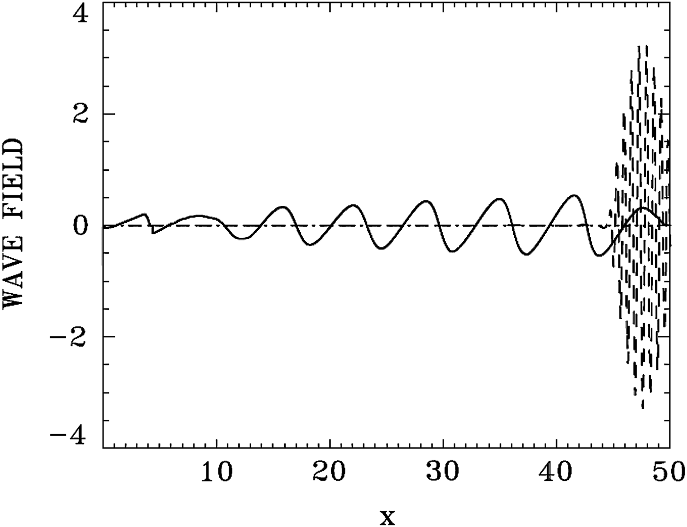
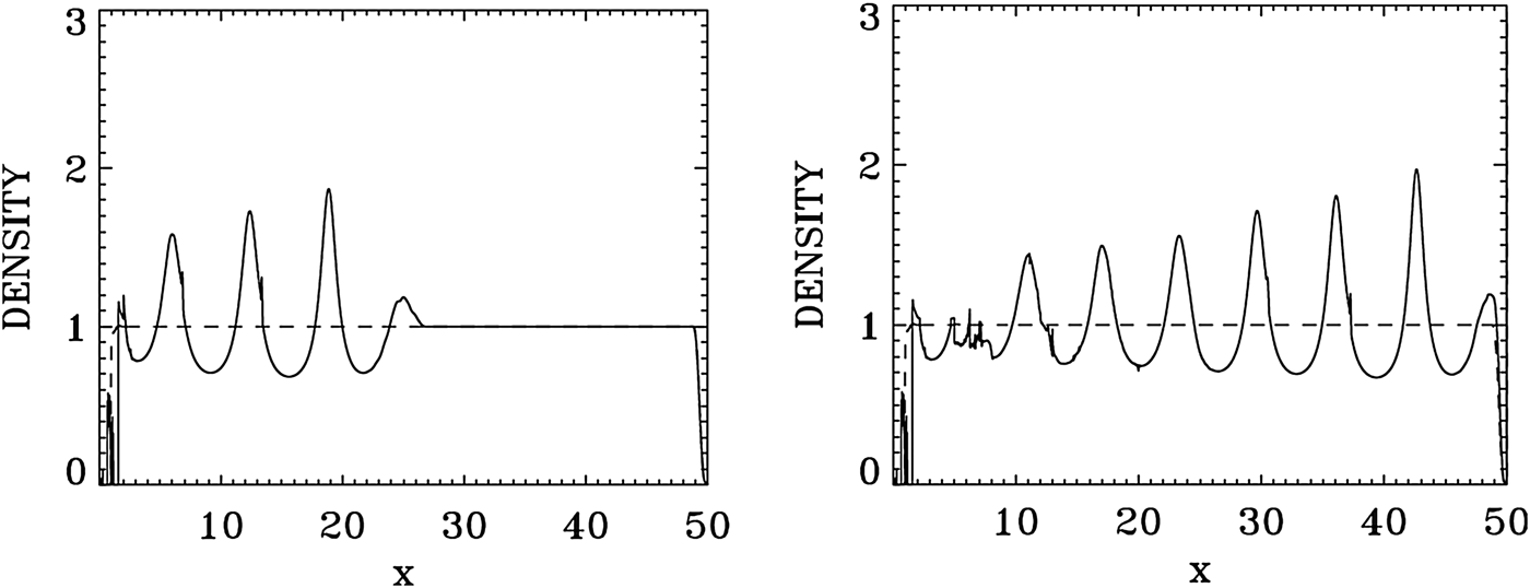
At t = 2π + 1, most of the entire envelope of length ≈ 2π of the forward propagating pulse has developed on the flat density part and is left to evolve self-consistently according to Eq. (5). Figure 36 shows the results for the laser pulse at t = 50 (broken curve, divided by 5 to allow visibility for the longitudinal electric field E _x), after crossing the domain and reaching the right boundary. It is followed by the wakefield E _x (full curve). There is little deformation of the EM pulse for the present set of parameters. Figure 37 shows the plot of the electron density (full curve), and the ion density (dashed curve). The modulation of the electron density is following the modulation of the wakefield in Figure 36. The ion density remains constant (if we accept a small deformation at the left of the domain due to the formation of a local sheath at the left edge). The longitudinal electric field E _x reaches in Figure 36 a peak of about 0.6.

Fig. 36. Laser pulse E ⁺/5 at t = 51 (broken curve, divided by 5 to allow visibility for the longitudinal electric field E _x), after crossing the domain and reaching the right boundary. It is followed by the wakefield E _x (full curve).

Fig. 37. Plot of the electron density (full curve) and the ion density (dashed curve) at t = 27 (left frame) and t = 51 (right frame).

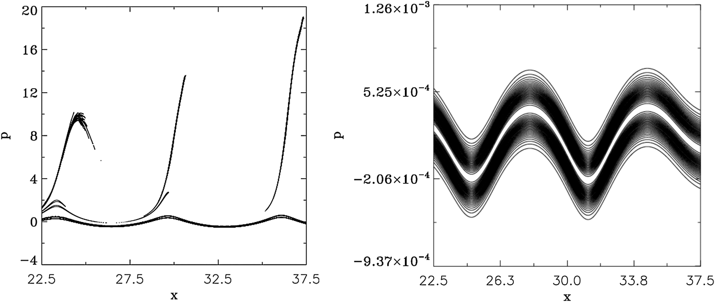
Figure 38 shows the phase-space plots for the electrons (left frame) and the ions (right frame) at t = 51, in the domain 22.5 < x < 37.5. Bunches of electrons detach from the bulk and are accelerated as beams around the peaks of the electric field (note that the contour levels of these accelerated beams are artificially enhanced in Figures 38 (left frame), in order to make them more visible). The ions density remained equal to 1 as mentioned in Figure 37, but are showing a modulation in phase space in Figure 38 (right frame), which follows the modulation of the electrons in Figure 38 (left frame).

Fig. 38. Phase-space contour plot in x = (22.5,37.5) of the electron distribution function (left frame) and the ion distribution function (right frame) at t = 51.