2. One-dimensional approach for diabatic flows with friction

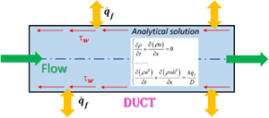
Generalised Euler partial differential equations (PDEs) for a 1-D unsteady viscous diabatic gaseous flow along a pipe with constant circular cross-section are given by (Bermudez, Lopez & Vasquez-Cendon Reference Bermudez, Lopez and Vasquez-Cendon2017)

(2.1) \begin{equation} \left. \begin{gathered} {\dfrac{{\partial \rho }}{{\partial t}} + \dfrac{{\partial (\rho u)}}{{\partial x}} = 0}\\ {\dfrac{{\partial (\rho u)}}{{\partial t}} + \dfrac{{\partial (p + \rho {\kern 1pt} {u^2})}}{{\partial x}} ={-} \dfrac{{4{\tau_w}}}{D}}\\ {\dfrac{{\partial (\rho {e^0})}}{{\partial t}} + \dfrac{{\partial (\rho {\kern 1pt} u{h^0})}}{{\partial x}} = \dfrac{{4{{\dot{q}}_f}}}{D}} \end{gathered} \right\},\end{equation}

where t is the time, x is the space coordinate, ρ, u and p are the cross-section averaged 1-D density, velocity and pressure, respectively, D is the pipe diameter ($A = {\rm \pi}/4{D^2}$ is the cross-section), e ⁰ is the stagnation internal energy (${e^0} = e + {u^2}/2$, where e is the internal energy), h ⁰ is the stagnation enthalpy (${h^0} = h + {u^2}/2$, where h is the enthalpy), τ_w is the wall friction shear stress and ${\dot{q}_f}$ is the heat flux exchanged by the fluid with the walls (${\dot{q}_f}$ is positive when the heat is supplied to the fluid).

Equation (2.1) differs from the standard set of Euler equations for an isentropic flow because the friction and heat exchange are added and evaluated as volume source terms (Hirsch Reference Hirsch2007; Maeda & Colonius Reference Maeda and Colonius2017), using the Darcy–Weisbach wall friction and convective heat transfer models. The wall friction stress is expressed by (White Reference White2015)

(2.2)\begin{equation}{\tau _w} = \frac{f}{2}\rho {\kern 1pt} {u|u|},\end{equation}

where the friction coefficient f can be expressed as a function of the Reynolds number ($Re = \rho uD/\mu$, with μ being the dynamical viscosity of the fluid) for a laminar flow and as a function of both Re and the relative roughness (ε/D, with ε being the average roughness of the wall) for a turbulent flow (Douglas et al. Reference Douglas, Gasiorek, Swaffield and Jack2005; Cheng Reference Cheng2008; White Reference White2015). The heat flux can be expressed as (Bejan Reference Bejan2013)

(2.3)\begin{equation}{\dot{q}_f} = \lambda ({T_w} - T),\end{equation}

where the film coefficient λ [W (m² K)⁻¹] is a function of the Reynolds and Prandtl (Pr) numbers, T is the cross-section averaged 1-D temperature of the fluid and T_w is the uniform wall temperature.

Equations (2.1)–(2.3) are completed with the following state equations of the gas:

(2.4) \begin{equation}\left. \begin{gathered} {p = \dfrac{{\gamma - 1}}{\gamma }\rho h,\quad h = {c_p}T}\\ {h = e + \dfrac{p}{\rho },\quad e = {c_v}T} \end{gathered} \right\},\end{equation}

where $\gamma = {c_p}/{c_v}$ is the ratio of the constant pressure specific heat (c_p) to the constant volume specific heat (c_v).

When steady-state flows are considered, the partial derivatives with respect to time vanish in (2.1), which can be reduced to the following system of nonlinear ordinary differential equations (ODEs) with respect to the independent variable x (Emmons Reference Emmons1958):

(2.5) \begin{equation}\left. \begin{gathered} {\dfrac{{\textrm{d}\dot{m}}}{{\textrm{d}x}} = 0}\\ {A\dfrac{{\textrm{d}p}}{{\textrm{d}x}} + \dot{m}\dfrac{{\textrm{d}u}}{{\textrm{d}x}} ={-} {\rm \pi} D{\tau_w}}\\ {\dot{m}\dfrac{{\textrm{d}{h^0}}}{{\textrm{d}x}} = {\rm \pi} D{{\dot{q}}_f}} \end{gathered} \right\},\end{equation}

where $\dot{m} = \rho Au$ is the mass flow rate through the pipe.

3. Exact 1-D solution for steady-state compressible viscous flows with constant $\dot{q}_{f}$

Let us consider a steady-state compressible viscous diabatic flow with constant ${\dot{q}_f}$ along a constant circular cross-section pipe. The mass conservation law in (2.5) can be rewritten as

(3.1)\begin{equation}\rho u = \frac{{\dot{m}}}{A} = \textrm{const}\end{equation}

Furthermore, the momentum balance and total energy laws in (2.5) can be rearranged as follows (the momentum balance and total energy equations are divided by Aρ and A, respectively, and (2.2) is used with $u > 0$):

(3.2)\begin{gather}\frac{{4f}}{D}\left( {\frac{{{u^2}}}{2}} \right) + \frac{A}{{\dot{m}}}u\frac{{\textrm{d}p}}{{\textrm{d}x}} + \frac{\textrm{d}}{{\textrm{d}x}}\left( {\frac{{{u^2}}}{2}} \right) = 0,\end{gather}

(3.3)\begin{gather}\frac{{\dot{m}}}{A}\frac{{\textrm{d}h}}{{\textrm{d}x}} + \frac{{\dot{m}}}{A}\frac{\textrm{d}}{{\textrm{d}x}}\left( {\frac{{{u^2}}}{2}} \right) = \frac{{4{{\dot{q}}_f}}}{D},\end{gather}

where f is a constant term, because $Re = \rho uD/\mu = 4\dot{m}/({\rm \pi} D\mu ) = \textrm{const}$ (the dependence of the dynamic viscosity of the fluid on T is neglected). The pressure can be expressed according to the following formula, which was obtained using the state equations of ideal gases, i.e. (2.4), in conjunction with (3.1):

(3.4)\begin{equation}p = \frac{{\gamma - 1}}{\gamma }\rho h = \frac{{\gamma - 1}}{\gamma }\frac{{\dot{m}}}{{Au}}h.\end{equation}

Therefore, the pressure gradient can be calculated by applying the chain rule:

(3.5)\begin{equation}\frac{{\textrm{d}p}}{{\textrm{d}x}} = \frac{{\dot{m}}}{{Au}}\frac{{\gamma - 1}}{\gamma }\frac{{\textrm{d}h}}{{\textrm{d}x}} - \frac{{\dot{m}}}{{A{u^2}}}\frac{{\gamma - 1}}{\gamma }h\frac{{\textrm{d}u}}{{\textrm{d}x}}.\end{equation}

By substituting (3.5) in (3.2) and taking (3.3) into account, we obtain

(3.6)\begin{equation}\frac{{4f}}{D}\left( {\frac{{{u^2}}}{2}} \right) - \frac{{\gamma - 1}}{{2\gamma }}h\frac{\textrm{d}}{{\textrm{d}x}}\left[ {\ln \left( {\frac{{{u^2}}}{2}} \right)} \right] - \frac{1}{\gamma }\frac{{\textrm{d}h}}{{\textrm{d}x}} ={-} \frac{{{{\dot{q}}_f}{\rm \pi} D}}{{\dot{m}}}.\end{equation}

Equation (3.3) can be divided by $\dot{m}/A$ and, because ${\dot{q}_f}$ is supposed to be a constant term (${\dot{q}_f}$ can be either positive or negative), it can easily be integrated with respect to x to obtain

(3.7)\begin{equation}h = h_1^0 + \frac{{{{\dot{q}}_f}{\rm \pi} D}}{{\dot{m}}}x - \frac{{{u^2}}}{2},\end{equation}

where $h_1^0$ is the stagnation enthalpy at ${x_1} = 0\ (h_1^0 = {c_p}T_1^0)$. Equation (3.7) can then be used to eliminate h from (3.6) and, after some analytical steps, the following equation can be achieved:

(3.8)\begin{align}\frac{{4f}}{D}\left( {\frac{{{u^2}}}{2}} \right) - \frac{{\gamma - 1}}{{2\gamma }}\left( {h_1^0 + \frac{{{{\dot{q}}_f}{\rm \pi} Dx}}{{\dot{m}}}} \right)\frac{\textrm{d}}{{\textrm{d}x}}\left[ {\ln \left( {\frac{{{u^2}}}{2}} \right)} \right] + \frac{{\gamma + 1}}{{2\gamma }}\frac{\textrm{d}}{{\textrm{d}x}}\left( {\frac{{{u^2}}}{2}} \right) = \frac{{1 - \gamma }}{\gamma }\frac{{{{\dot{q}}_f}{\rm \pi} D}}{{\dot{m}}}.\end{align}

Equation (3.8) is a nonlinear ODE with a single unknown function, that is, the kinetic energy per unit of mass (u ²/2). By changing the variable (let us use the letter ‘t’ for the new variable because there is no time in the rest of the current section)

(3.9)\begin{equation}t: = \ln \left( {\frac{{{u^2}}}{2}} \right),\end{equation}

and performing some algebraic manipulation, (3.8) can finally be converted into the following heterogeneous linear ODE:

(3.10)\begin{equation}\frac{{\textrm{d}x}}{{\textrm{d}t}} + a(t)x = b(t),\end{equation}

where

(3.11) \begin{equation}a(t) ={-} \left( {\frac{{\displaystyle\frac{{\gamma - 1}}{{2\gamma }}\frac{{{{\dot{q}}_f}{\rm \pi} D}}{{\dot{m}}}}}{{\displaystyle\frac{{4f}}{D}{e^t} + \displaystyle\frac{{\gamma - 1}}{\gamma }\frac{{{{\dot{q}}_f}{\rm \pi} D}}{{\dot{m}}}}}} \right)\quad b(t) = \left( {\frac{{\displaystyle\frac{{\gamma - 1}}{{2\gamma }}h_1^0 - \frac{{\gamma + 1}}{{2\gamma }}{e^t}}}{{\displaystyle\frac{{4f}}{D}{e^t} + \frac{{\gamma - 1}}{\gamma }\frac{{{{\dot{q}}_f}{\rm \pi} D}}{{\dot{m}}}}}} \right).\end{equation}

It is known that any linear first-order ODE with variable coefficients can be solved using Lagrange's method of variation of the constants (Hairer, Norsett & Wanner Reference Hairer, Norsett and Wanner1993). The general solution to (3.10) takes the form

(3.12)\begin{equation}x(t) = {\textrm{e}^{ - A(t)}}\left[ {\int {b(t)\,{\textrm{e}^{A(t)}} + C} } \right],\end{equation}

where $A(t) = \int {a(t)\,\textrm{d}t} $ is a primitive function of a(t) and C is a constant value that can be calculated by assigning a boundary condition to the Cauchy problem.

By using the above expression for a(t), one obtains (the integral $\int {a(t)\,\textrm{d}t} $ is of the form $- 1/2\int {B/({\textrm{e}^t} + B)\,\textrm{d}t} = 1/2\ln (|{e^t} + B|/{e^t})$, where B is a general constant term)

(3.13) \begin{equation}A(t) ={-} \int {\left( {\frac{{\displaystyle\frac{{\gamma - 1}}{{2\gamma }}\frac{{{{\dot{q}}_f}{\rm \pi} D}}{{\dot{m}}}}}{{\displaystyle\frac{{4f}}{D}{e^t} + \frac{{\gamma - 1}}{\gamma }\frac{{{{\dot{q}}_f}{\rm \pi} D}}{{\dot{m}}}}}} \right)} \,\textrm{d}t = \ln \frac{{{{\left|{{\textrm{e}^t} + \displaystyle\frac{{\gamma - 1}}{\gamma }\frac{{{{\dot{q}}_f}{\rm \pi}{D^2}}}{{4f\dot{m}}}} \right|}^{1/2}}}}{{{\textrm{e}^{t/2}}}},\end{equation}

and consequently (3.12), after some algebraic manipulation and recalling that $t = \ln ({u^2}/2)$, becomes

(3.14) \begin{align} x &= \left\{ {sgn\left( {\dfrac{{{u^2}}}{2} + \dfrac{{\gamma - 1}}{\gamma }\dfrac{{{{\dot{q}}_f}{\rm \pi}{D^2}}}{{4f\dot{m}}}} \right)\int {\left[ {\dfrac{{\dfrac{{\gamma - 1}}{\gamma }\dfrac{D}{{8f}}h_1^0 - \dfrac{{\gamma + 1}}{\gamma }\dfrac{D}{{8f}}\dfrac{{{u^2}}}{2}}}{{{{\left( {\dfrac{{{u^2}}}{2}} \right)}^{3/2}}{{\left|{{\kern 1pt} \dfrac{{{u^2}}}{2} + \dfrac{{\gamma - 1}}{\gamma }\dfrac{{{{\dot{q}}_f}{\rm \pi}{D^2}}}{{4f\dot{m}}}} \right|}^{1/2}}}}} \right]d\left( {\dfrac{{{u^2}}}{2}} \right) + C} } \right\}\nonumber\\ &\quad \times\dfrac{{{{\left( {\dfrac{{{u^2}}}{2}} \right)}^{1/2}}}}{{{{\left|{{\kern 1pt} \dfrac{{{u^2}}}{2} + \dfrac{{\gamma - 1}}{\gamma }\dfrac{{{{\dot{q}}_f}{\rm \pi}{D^2}}}{{4f\dot{m}}}} \right|}^{1/2}}}},\end{align}

where sgn represents the signum function, which extracts the sign of the quantity to which it is applied. The indefinite integral should be resolved to obtain an effective solution to the fluid dynamics problem in closed form. As a result of the change in variable $w = \sqrt {{u^2}/2} $, one obtains

(3.15) \begin{equation}\int {\left[ {\dfrac{{\dfrac{{\gamma - 1}}{\gamma }\dfrac{{D{\kern 1pt} }}{{8f}}h_1^0 - \dfrac{{\gamma + 1}}{\gamma }\dfrac{D}{{8f}}\dfrac{{{u^2}}}{2}}}{{{{\left|{{\kern 1pt} \dfrac{{{u^2}}}{2} + \dfrac{{\gamma - 1}}{\gamma }\dfrac{{{{\dot{q}}_f}{\rm \pi}{D^2}}}{{4f\dot{m}}}} \right|}^{1/2}}{{\left( {\dfrac{{{u^2}}}{2}} \right)}^{3/2}}}}} \right]d\left( {\dfrac{{{u^2}}}{2}} \right) = \int {\left[ {\dfrac{{\dfrac{{\gamma - 1}}{\gamma }\dfrac{{D{\kern 1pt} }}{{4f}}h_1^0 - \dfrac{{\gamma + 1}}{\gamma }\dfrac{D}{{4f}}{w^2}}}{{{w^2}{{\left|{{w^2} + \dfrac{{\gamma - 1}}{\gamma }\dfrac{{{{\dot{q}}_f}{\rm \pi}{D^2}}}{{4f\dot{m}}}} \right|}^{1/2}}}}} \right]\,\textrm{d}w} } .\end{equation}

The indefinite integral on the right-hand side of (3.15) can be interpreted as

(3.16) \begin{align}\int {\left[ {\dfrac{{\dfrac{{\gamma - 1}}{\gamma }\dfrac{{D{\kern 1pt} }}{{4f}}h_1^0 - \dfrac{{\gamma + 1}}{\gamma }\dfrac{D}{{4f}}{w^2}}}{{{w^2}{{\left|{{w^2} + \dfrac{{\gamma - 1}}{\gamma }\dfrac{{{{\dot{q}}_f}{\rm \pi}{D^2}}}{{4f\dot{m}}}} \right|}^{1/2}}}}} \right]\,\textrm{d}w} &\Rightarrow \int {\left[ {\dfrac{{F - G{w^2}}}{{{w^2}\sqrt {|{w^2} + E|} }}} \right]\,\textrm{d}w}\nonumber\\ & = \int {\left[ {\dfrac{F}{{{w^2}\sqrt {|{w^2} + E|} }} - \dfrac{G}{{\sqrt {|{w^2} + E|} }}} \right]\,\textrm{d}w} ,\end{align}

where $E = (\gamma - 1){\dot{q}_f}{\rm \pi}{D^2}/(4\gamma f\dot{m})$, $F = (\gamma - 1)Dh_1^0/(4\gamma f)$ and $G = (\gamma + 1)D/(4\gamma f)$ are constant terms in the considered problem, that is, they are independent of w.

Let us suppose that ${w^2} + E > 0\,\forall x$ ($\; {\dot{q}_f}$ can still be either positive or negative with this hypothesis). The initial integral in (3.16) is split into two indefinite integrals that can be expressed in terms of the following elementary functions (Dwight Reference Dwight1961):

(3.17)\begin{equation}\left. \begin{gathered} {\int {\dfrac{G}{{\sqrt {{w^2} + E} }}\,\textrm{d}w} = {\kern 1pt} G\ln \dfrac{{w + \sqrt {{w^2} + E} }}{{\sqrt {|E|} }}}\\ {\int {\dfrac{F}{{{w^2}\sqrt {{w^2} + E} }}\,\textrm{d}w} ={-} \dfrac{F}{E}\dfrac{{\sqrt {{w^2} + E} }}{w}} \end{gathered} \right\}.\end{equation}

By considering (3.14)–(3.17), the general analytical solution to (3.8) is provided explicitly as $x = x({u^2}/2)$:

(3.18) \begin{align}x ={-} \dfrac{{\dot{m}h_1^0}}{{{{\dot{q}}_f}{\rm \pi} D}} + \left\{ {C - \dfrac{{\gamma + 1}}{\gamma }\dfrac{D}{{4f}}\ln \left[ {\dfrac{{\sqrt {\dfrac{{{u^2}}}{2}} + \sqrt {\dfrac{{{u^2}}}{2} + \dfrac{{\gamma - 1}}{\gamma }\dfrac{{{{\dot{q}}_f}{\rm \pi}{D^2}}}{{4f\dot{m}}}} }}{{\sqrt {\dfrac{{\gamma - 1}}{\gamma }\dfrac{{\textrm{|}{{\dot{q}}_f}|{\rm \pi} {D^2}}}{{4f\dot{m}}}} }}} \right]} \right\}{\kern 1pt} \dfrac{{\sqrt {\dfrac{{{u^2}}}{2}} }}{{\sqrt {\dfrac{{{u^2}}}{2} + \dfrac{{\gamma - 1}}{\gamma }\dfrac{{{{\dot{q}}_f}{\rm \pi}{D^\textrm{2}}}}{{4f\dot{m}}}} }}.\end{align}

Once the value of integration constant C has been determined (cf. § 3.1), (3.18) becomes well defined. The 1-D T versus x distribution can then be expressed in parametric form using (3.7) and (3.18), where the kinetic energy per unit of mass of the fluid is the parameter:

(3.19) \begin{equation}\left. \begin{gathered} {T = T_1^0 + \dfrac{{{{\dot{q}}_f}{\rm \pi} D}}{{\dot{m}{\kern 1pt} {c_p}}}x\left( {\dfrac{{{u^2}}}{2}} \right) - \dfrac{{{u^2}}}{{2{c_p}}}}\\ {x = x\left( {\dfrac{{{u^2}}}{2}} \right)} \end{gathered} \right\}.\end{equation}

Furthermore, the density and pressure distributions, with respect to x, can be expressed as parametric equations: ρ(x) is obtained by coupling (3.18) with (3.1) and p(x) is achieved by linking (3.18) with both (3.4) and (3.7).

Finally, the Mach number distributions with respect to x can also be determined in parametric form by using (3.18) and (3.19) as well as the formula $Ma = \sqrt {{u^2}/(\gamma RT)}$.

The exact solutions and the corresponding analytical variants for the w ² + E = 0 and w ² + E < 0 cases are discussed in the appendix of the paper to avoid excessive fragmentation of the theoretical development with the introduction of too many details. Although these cases are essential to complete the exact solution, the main objective of the present paper is to highlight a methodology that can be used for the analytical treatment and physical interpretation of compressible viscous diabatic flows. It therefore appeared more efficient to present the procedure by only making preliminarily reference to the ${w^2} + E > 0\,\forall x$ condition and then extending the method to the other cases in the appendix.

3.1. Input data for the physical problem and determination of constant C

The constant heat flux is regarded as a given value in the present approach. In fact, the heat transfer power $\dot{Q}\; $ (either positive or negative), exchanged entirely through the walls of the circular pipe of assigned length L and diameter D, should be provided as an input value for the physical problem, and the heat flux per unit of area can thus be defined using the formula ${\dot{q}_f} = \dot{Q}/({\rm \pi} DL)$.

Furthermore, three independent boundary conditions are required to determine the values of the constant terms $h_1^0$, $\dot{m}$ and C in (3.18). These three boundary conditions, for the numerical solution of the unsteady PDE problem given by (2.1)–(2.3), should be provided following precise rules, according to the characteristic theory of systems of hyperbolic partial differential equations (Toro Reference Toro2009).

It is not necessary to pursue this theory in the present case because a steady-state problem is being analysed. In fact, the three input data values can be assigned at the x ₁ = 0 and x ₂ = L boundaries, without any constraints (Urata Reference Urata2013), although the easiest choice is to provide the mass flow rate and total temperature as well as the fluid velocity at the inlet of the pipe (x ₁ = 0). However, we here follow the characteristic line approach because it is exhaustive in illustrating how the available data at the boundaries can be used to determine the analytical solution.

According to the characteristic line theory, when the flow through the pipe is subsonic, two boundary conditions should be assigned at the pipe inlet, namely $T_1^0$ and total pressure $(p_1^0)$, while one boundary datum should be provided at the pipe exit (x ₂ = L), namely the static pressure (p_V) of the pipe downstream environment.

A shooting procedure can therefore be arranged: a tentative value of Ma ₁ can be selected, and $u_1^2/2$ and $\dot{m}$ can then be determined using the following equations, which refer to an isentropic evolution from the stagnation conditions to state 1 (Zucker & Biblarz Reference Zucker and Biblarz2002):

(3.20) \begin{equation}\left. \begin{gathered} {\dfrac{{u_1^2}}{2} = {c_p}T_1^0Ma_1^2{{\left( {\dfrac{2}{{\gamma - 1}} + Ma_1^2} \right)}^{ - 1}}}\\ {\dot{m} = \dfrac{{p_1^0}}{{\sqrt {RT_1^0} }}A\sqrt \gamma M{a_1}{{\left( {1 + \dfrac{{\gamma - 1}}{2}Ma_1^2} \right)}^{ - (\gamma + 1)/2(\gamma - 1)}}} \end{gathered} \right\}.\end{equation}

The constant C value can then be calculated by solving (3.18) under the condition ${u^2}/2 = u_1^2/2$ at x = x ₁ = 0:

(3.21) \begin{align}C = \dfrac{{\dot{m}{\kern 1pt} h_1^0}}{{{{\dot{q}}_f}{\rm \pi} D}}\dfrac{{\sqrt {\dfrac{{u_1^2}}{2} + \dfrac{{\gamma - 1}}{\gamma }\dfrac{{{{\dot{q}}_f}{\rm \pi}{D^2}}}{{4f\dot{m}}}} }}{{\sqrt {\dfrac{{u_1^2}}{2}} }} + \dfrac{{\gamma + 1}}{\gamma }\dfrac{D}{{4f}}\ln \left[ {\dfrac{{\sqrt {\dfrac{{u_1^2}}{2}} + \sqrt {\dfrac{{u_1^2}}{2} + \dfrac{{\gamma - 1}}{\gamma }\dfrac{{{{\dot{q}}_f}{\rm \pi}{D^2}}}{{4f\dot{m}}}} }}{{\sqrt {\dfrac{{\gamma - 1}}{\gamma }\dfrac{{\textrm{|}{{\dot{q}}_f}{|{\rm \pi} }{D^2}}}{{4f\dot{m}}}} }}} \right].\end{align}

Equation (3.18), with C given by (3.21), can be employed to determine the $u_2^2/2$ at x ₂ = L value. Furthermore, density ρ ₂ can be evaluated from (3.1), which is applied for x ₂ = L, and (3.7) can be used to calculate h ₂ at x ₂ = L.

Finally, pressure p ₂ can be calculated as a function of ρ ₂ and h ₂ using (3.4). If the thus determined p ₂ value is equal to the provided boundary datum p_V, the guessed value of Ma ₁ is suitable, otherwise the shooting procedure should be repeated selecting new values of Ma ₁ until consistency with downstream boundary pressure p_V is achieved. At the end of the procedure, C has been evaluated accurately and (3.18) is therefore ready for use. When the flow through the pipe is supersonic, the hyperbolic PDE theory requires that all three boundary conditions are given at the pipe inlet, namely $T_1^0,p_1^0$ and Ma ₁ at x ₁ = 0. In this case, both $\dot{m}$ and $u_1^2/2$ can be evaluated directly using (3.20), and C can then be determined using (3.21); hence, (3.18) is completely defined.

3.2. Dimensionless representation of the exact solution

Equations (3.18) and (3.21), the physical domain and the required boundary conditions of the problem (for the sake of simplicity, let us here suppose that such boundary conditions are provided by the $h_1^0$, $\dot{m}$ and $u_1^2/2$ values) involve eight dimensional sizes, that is, x, $\dot{m}$, $h_1^0$, D, u ²/2, $u_1^2/2$, L, $\; {\dot{q}_f}$, and two dimensionless parameters, that is, γ and f. Because both mechanical and thermal quantities are involved in the problem, the rank of the dimensional problem is equal to four, i.e. m, s, kg and K are required as measurement units to express all the quantities that appear in the problem.

According to Buckingham's theorem (Yarin Reference Yarin2012), it is possible to express the solution and boundary conditions in terms of (8 + 2) − 4 = 6 dimensionless groups. The dimensionless representation of the solution can be useful to clearly identify the physical factors that drive the analysed phenomenon.

If (3.18) is multiplied by f/D_h, where D_h is the ratio of cross-sectional area to wetted perimeter (D_h = D/4 for circular sections), and ${\dot{q}_f}$ is replaced by the total heat transfer power per unit of mass flow rate, namely q, which is defined as $q\; = {\dot{q}_f}{\rm \pi} DL/\dot{m}$, the following dimensionless equation can be obtained after some algebraic manipulation $({C^\ast }: = Cf/{D_h})$:

(3.22) \begin{align}f\dfrac{x}{{{D_h}}} &={-} \dfrac{{h_1^0}}{q}f\dfrac{L}{{{D_h}}} + \left\{ {{C^\ast } - \dfrac{{\gamma + 1}}{\gamma }\ln \left[ {\dfrac{{\sqrt {\dfrac{{{u^2}}}{{2|q|}}} + \sqrt {\dfrac{{{u^2}}}{{2|q|}} + sgn({{\dot{q}}_f})\dfrac{{\gamma - 1}}{\gamma }\dfrac{{{D_h}}}{{fL}}} }}{{\sqrt {\dfrac{{\gamma - 1}}{\gamma }\dfrac{{{D_h}}}{{{\kern 1pt} fL}}} }}} \right]} \right\}\nonumber\\ &\quad \times \dfrac{{\sqrt {\dfrac{{{u^2}}}{{2|q|}}} }}{{\sqrt {\dfrac{{{u^2}}}{{2|q|}} + sgn({{\dot{q}}_f})\dfrac{{\gamma - 1}}{\gamma }\dfrac{{{D_h}}}{{{\kern 1pt} fL}}} }}.\end{align}

Let us now define the following dimensionless number

(3.23)\begin{equation}{\varPi _L} = \frac{{{{\dot{q}}_f}{\rm \pi} DL}}{{\dot{m}h_1^0}} = \frac{q}{{h_1^0}} = \frac{{h_2^0 - h_1^0}}{{h_1^0}} = \frac{{T_2^0}}{{T_1^0}} - 1,\end{equation}

which expresses the ratio of the total heat transfer power (over length L of the duct) to the flux of the total enthalpy at the pipe inlet, namely $\dot{m}h_1^0$. When the heat transfer is null, the total enthalpy is conserved along the pipe, hence Π_L = 0 and Fanno's model is obtained. In general, a higher modulus of Π_L (${\dot{q}_f}$ can be either positive or negative) leads to a greater impact of the heat transfer on the flow evolution.

The term ${u^2}/2|q|$ on the right-hand side of (3.22) can be developed by taking (3.7) and (3.23) into account:

(3.24)\begin{equation}\quad \frac{{{u^2}}}{{2|q|}} = \frac{{{u^2}}}{{2{c_p}|T_2^0 - T_1^0|}} = C{r^2}\frac{{{T^0}/T_1^0}}{{|T_2^0/T_1^0 - 1|}} = \frac{{C{r^2}}}{{|{\varPi _L}|}}\left( {1 + {\Pi_L}\frac{x}{L}} \right),\end{equation}

where $Cr = u/\sqrt {2{c_p}{T^0}} $ is the Crocco number and T ⁰ is the stagnation temperature at section x.

By substituting (3.24) and (3.23) in (3.22), and after some algebraic steps, one can obtain the following implicit dimensionless representation of the solution:

(3.25) \begin{align}fx/{D_h} &={-} \frac{1}{\varGamma } + \left\{ {{C^\ast } - \ln {{\left[ {\frac{{Cr\sqrt {1 + \varGamma fx/{D_h}} + \sqrt {C{r^2}(1 + \varGamma fx/{D_h}) + \varGamma \frac{{\gamma - 1}}{\gamma }} }}{{\sqrt {|\varGamma |\frac{{\gamma - 1}}{\gamma }} }}} \right]}^{{\kern 1pt} (\gamma + 1)/\gamma }}} \right\}\nonumber\\ &\quad \times\frac{{Cr\sqrt {1 + \varGamma fx/{D_h}} }}{{\sqrt {C{r^2}(1 + \varGamma fx/{D_h}) + \varGamma \frac{{\gamma - 1}}{\gamma }} }},\end{align}

where

(3.26)\begin{align}\Gamma = \frac{{{\varPi _L}}}{{(fL/{D_h})}},\quad {C^\ast } = \frac{1}{\varGamma }\frac{{\sqrt {Cr_1^2 + \varGamma \frac{{\gamma - 1}}{\gamma }} }}{{C{r_1}}} + \ln {\left[ {\frac{{C{r_1} + \sqrt {Cr_1^2 + \varGamma \frac{{\gamma - 1}}{\gamma }} }}{{\sqrt {|\varGamma |\frac{{\gamma - 1}}{\gamma }} }}} \right]^{{\kern 1pt} (\gamma + 1)/\gamma }}.\end{align}

A practical way of obtaining an explicit dependence of $fx/{D_h}$ on Cr would be to define the Crocco number as $= u/\sqrt {2{c_p}T_1^0} $, as is done in some fluid machinery textbooks when the stagnation temperature is variable along the component. However, this is not the preferred choice for theoretical gas dynamics and, above all, the definition of Cr that adopts $T_1^0$ would not allow $fx/{D_h}$ to explicitly depend on the Mach number.

Six dimensionless factors appear in (3.25): $fx/{D_h}$, Cr, fL/D_h, Π_L, γ and Cr ₁ (only $fx/{D_h}$ and Cr are variable with x, whereas the other factors are fixed parameters of the solution). The Π_L group takes thermal effects into account and is also relevant for a Rayleigh flow, while the fL/D_h and $fx/{D_h}$ terms, which include the friction coefficient and the aspect ratio of either the pipe or a portion of the pipe, account for the friction effect and are noteworthy groups for Fanno's flow (Shapiro Reference Shapiro1953).

Another notable implicit dimensionless representation, which is an alternative to (3.25), is given by

(3.27) \begin{align}{\varPi _x} &={-} 1 + \left\{ {{C^\ast } - \ln {{\left[ {\frac{{Cr\sqrt {1 + {\Pi_x}} + \sqrt {C{r^2}(1 + {\Pi_x}) + \varGamma \frac{{\gamma - 1}}{\gamma }} }}{{\sqrt {|\varGamma |\frac{{\gamma - 1}}{\gamma }} }}} \right]}^{(\gamma + 1)/\gamma }}} \right\}\nonumber\\ &\quad \times\frac{{Cr\varGamma \sqrt {1 + {\varPi _x}} }}{{\sqrt {C{r^2}(1 + {\varPi _x}) + \varGamma \frac{{\gamma - 1}}{\gamma }} }},\end{align}

where ${\varPi _x} = {\dot{q}_f}{\rm \pi} D{\kern 1pt} x/\dot{m}h_1^0$, and constant C* has the same expression as that which is valid for (3.25).

The six dimensionless factors in (3.27) are Π_x, Cr, fL/D_h, Π_L, γ and Cr ₁. Therefore, variable $fx/{D_h}$, which appears in (3.25), has been substituted with variable Π_x in (3.27), on the basis of the ${\varPi _x} = \varGamma fx/{D_h}$ relation.

Finally, the Crocco number can be expressed in both (3.25) and (3.27) as a function of γ and the Mach number, according to the formula

(3.28)\begin{equation}Cr = \frac{{Ma}}{{\sqrt {M{a^2} + 2/(\gamma - 1)} }}.\end{equation}

Once (3.28) has been substituted in either (3.25) or (3.27), new implicit dimensionless solutions, which link either $fx/{D_h}$ or Π_x, respectively, to Ma, can be determined for compressible viscous diabatic flows (fL/D_h, Π_L, Ma ₁ and γ will be the fixed parameters of the solutions). The advantage of these new dimensionless representations is that they include Ma, which is also a fundamental dimensionless variable in the Fanno and Rayleigh models. This facilitates any comparison between the newly developed analytical model and simple flow analytical models that lead to dimensionless explicit relations between Ma and either $fx/{D_h}$ (Fanno's model) or Π_x (Rayleigh's model).

The dimensionless representation obtained by coupling (3.25) and (3.28) is suitable for a comparison with the Fanno flow and can therefore be referred to as Fanno's dimensionless mode representation of the compressible viscous diabatic flow.

Instead, the dimensionless representation obtained by coupling (3.27) and (3.28) is suitable for comparison with the Rayleigh flow and can be referred to as Rayleigh's dimensionless mode representation of the compressible viscous diabatic flow. A fundamental role is played by quantity $\varGamma$ in both of these representations, which accounts for the relative importance of the heat transfer and friction groups of the whole pipe during the evolution of the viscous diabatic flow.

4. Validation of the exact solutions with constant ${\dot{q}_{f}}$

The previously developed analytical solutions were validated through a comparison with the corresponding time asymptotic distributions, which resulted from the numerical solution of (2.1), (2.2) and (2.4). The expression of ${\dot{q}_f}$ in the PDE numerical model was regarded as a constant value.

The PDEs were discretised using a finite volume method, according to a flux vector splitting technique (Laney Reference Laney1998; Toro Reference Toro2009) that applies a high-resolution upwind discretisation scheme with a Van Leer flux limiter (Le Veque Reference Le Veque1990). The spatial mesh size, namely Δx, was selected to guarantee a grid independent numerical solution. The time step, namely Δt, was set to obtain σ = 0.9, where $\sigma = |u + \sqrt {\gamma RT} {|_{max}}\Delta t/\Delta x$ is the instantaneous Courant number (Tannehill, Anderson & Pletcher Reference Tannehill, Anderson and Pletcher1997) and $|u + \sqrt {\gamma RT} {|_{max}}$ is the maximum modulus of the $u(x,t) + \sqrt {\gamma RT(x,t)} $ numerical space distribution at each fixed time instant.

The boundary conditions of the PDEs were provided according to the characteristic theory for hyperbolic problems. Therefore, the stagnation temperature and stagnation pressure were assigned to the pipe inlet section for subsonic flows, whereas static pressure was assigned to the pipe downstream environment. Three boundary data, namely stagnation temperature, stagnation pressure and Mach number, were instead assigned to the pipe inlet for supersonic flows, and no boundary data were provided for the pipe exit.

Figures 1 and 2 refer to a steady-state (or time asymptotic for the numerical solution) viscous diabatic flow with a positive constant heat flux $({\dot{q}_f} = \textrm{const} > 0)$: figure 1 reports the results of a validation test for a subsonic flow, whereas figure 2 reports the results of a validation test for a supersonic flow.

Figure 1. Validation test for the exact solution with a positive constant heat flux for a subsonic flow. Test conditions: L = 50 cm, D = 0.98 cm, $p_1^0 = 5\;\textrm{bar}$, $T_1^0 = 570\;\textrm{K}$, p_V = 2.5 bar, f = 4 × 10⁻³, ${\dot{q}_f} = 6 \times {10^5}\;\textrm{W}\;{\textrm{m}^{ - 2}}$, γ = 1.4, R = 287 J (kg K)⁻¹, Δx = 1 mm $(\dot{m} = 41.28\;\textrm{g}\;{\textrm{s}^{ - 1}})$.

Figure 2. Validation test for the exact solution with a positive constant heat flux for a supersonic flow. Test conditions: L = 67.16 cm, D = 2.5 cm, $p_1^0 = 3\;\textrm{bar}$, $T_1^0 = 800\;\textrm{K}$, Ma ₁ = 2.5, f = 3 × 10⁻³, ${\dot{q}_f} = 10^{5}\;\textrm{W}\;{\textrm{m}^{-2}}$, γ = 1.4, R = 287 J (kg K)⁻¹, Δx = 1 mm $(\dot{m} = 79.81\;\textrm{g}\;{\textrm{s}^{ - 1}})$.

The analytical solutions are plotted with either a continuous line (velocity) or a dashed line (temperature): the unidimensional diagrams of the velocity were calculated by applying (3.18), whereas the temperature versus x distributions were determined using the parametric relations in (3.19). The numerical solutions are reported with symbols. The constant C in (3.18) was calculated with the shooting procedure illustrated in § 3.1 for the subsonic flow case, whereas C was determined directly, using (3.20) and (3.21), for the supersonic flow case.

Furthermore, figure 3 reports a validation test for a subsonic flow for the case of a negative constant heat flux $({\dot{q}_f} = \textrm{const} < 0,{w^2} + E > 0\,\forall x)$ and according to the boundary conditions specified in the caption.

Figure 3. Validation test for the analytical solution with a negative constant heat flux for a subsonic flow. Test conditions: L = 51 cm, D = 0.7 cm, $p_1^0 = 6\;\textrm{bar}$, $T_1^0 = 600\;\textrm{K}$, p_V = 2.44 bar, f = 5 × 10⁻³, ${\dot{q}_f} ={-} {10^5}\;\textrm{W}\;{\textrm{m}^{ - 2}}$, γ = 1.4, R = 287 J (kg K)⁻¹, Δx = 1 mm $(\dot{m} = 27.6\;\textrm{g}\;{\textrm{s}^{ - 1}})$.

As can be inferred, each graph in figures 1–3 shows an excellent agreement between the corresponding curves, and this is clear proof of the physical consistency of the determined exact solutions for the ${\dot{q}_f} = \textrm{const}$ case.

5. Physical discussion of the exact solutions with constant ${\dot{q}_{f}}$

5.1. Results in the enthalpy–entropy diagram and identification of choking conditions

A physical interpretation of the developed exact solutions for compressible viscous diabatic flows in the ${\dot{q}_f} = \textrm{const}$ case can be provided by analysing the enthalpy–entropy diagrams, as is usually done when presenting Fanno's and Rayleigh's models.

The h–s curves can be calculated by applying (3.18), (3.19), (3.7) and (3.4), together with the state equation for entropy, that is, $s = {c_p}\ln (T/T_1^0) - R\ln (p/p_1^0)$, where $s(p_1^0,T_1^0)$ is taken as null.

Figure 4 reports h–s curves that refer to initially subsonic flows for the ${\dot{q}_f} > 0$ case. All the curves, except that plotted with a dash–dotted line without symbols, are characterised by the same conditions at the pipe inlet (point at s = 0), namely $T_1^0$, $p_1^0$, D and Ma ₁, and thus by the same mass flow rate, which are specified in the caption.

Figure 4. Entropy–enthalpy curves for an initially subsonic flow. The conditions for the tests in the legend: D = 0.98 cm, $p_1^0 = 5\;\textrm{bar}$, $T_1^0 = 570\;\textrm{K}$, Ma ₁ = 0.41, γ = 1.4, R = 287 J (kg K)⁻¹, $(\dot{m} = 41.28\;\textrm{g}\;{\textrm{s}^{ - 1}})$.

The differences between the curves with the same flow rate arise because different couples of f and ${\dot{q}_f}$ values have been applied (these values are quoted in the legend). In particular, the continuous solid line without symbols refers to the same $T_1^0$, $p_1^0$, $\dot{m}$, f, D and ${\dot{q}_f}$ conditions as those in the validation test shown in figure 1. The dash–dotted curved line without symbols refers to the same $T_1^0$, $p_1^0$, D conditions as those of the other curves and to the same f, ${\dot{q}_f}$ values as the continuous line without symbols, but features an increased specific flow rate, i.e. a larger value of ${{\dot{m}} / A}$ and thus a higher Ma ₁.

Figure 5 plots a similar graph to that shown in figure 4, but for supersonic viscous diabatic flows: the curve plotted with a continuous line without any symbols refers to the same $T_1^0$, $p_1^0$, $\dot{m}$, f, D and ${\dot{q}_f}$ conditions as in the validation test of figure 2. The f and positive ${\dot{q}_f}$ values pertaining to the other curves plotted with symbols, which refer to the same $T_1^0$, $p_1^0$, D and $\dot{m}$ conditions as those for the continuous curve without symbols, are also reported in the legend. Furthermore, a portion of the curve that refers to a larger value of ${{\dot{m}} / A}$ has been reported with a dash–dotted line to show the effect of an increased specific flow rate on the h-s curves, as in figure 4.

Figure 5. Entropy–enthalpy curves for an initially supersonic flow. The conditions for the tests in the legend: D = 2.5 cm, $p_1^0 = 3\;\textrm{bar}$, $T_1^0 = 800\;\textrm{K}$, Ma ₁ = 2.5, γ = 1.4, R = 287 J (kg K)⁻¹, $(\dot{m} = 79.81\;\textrm{g}\;{\textrm{s}^{ - 1}})$.

While the Fanno and Rayleigh h–s curves are unique, once the stagnation point at the pipe inlet and ${{\dot{m}} / A}$ have been assigned, infinite h–s curves for the viscous diabatic flow, which depend on the f and ${\dot{q}_f}$ values, as shown in figures 4 and 5, can exist.

Because a positive heat flux is considered in both figures 4 and 5, s can only increase when the flow goes through the pipe (dx > 0). This is confirmed by the following entropy equation:

(5.1)\begin{equation}T\,\textrm{d}s = \delta q + \delta {l_w} = \frac{{{{\dot{q}}_f}{\rm \pi} D}}{{\dot{m}}}\,\textrm{d}x + \frac{{2f}}{D}{u^2}\,\textrm{d}x\end{equation}

Therefore, the increasing entropy gives the direction of the flow evolution along any h–s curve in figures 4 and 5. Any point to the right of an initial point at s = 0 along a curve, in either figure 4 or 5, corresponds to the state at the end of a pipe of a certain length L.

For example, the point at h ≈ 700 kJ kg⁻¹ along the continuous-line curve in figure 4 corresponds to the subsonic flow condition at the end of the pipe considered in figure 1 (L = 50 cm, p_V = 2.5 bar), whereas the point at h ≈ 700 kJ kg⁻¹ along the continuous-line curve in figure 5 corresponds to the supersonic flow condition at the end of the pipe considered in figure 2 (L = 67.16 cm, p_V = 0.56 bar).

In figure 4, as the flow proceeds along the h–s curve, both the velocity and the Mach number increase, while the pressure decreases. Instead, in figure 5, as the entropy increases, both the velocity and the Mach number reduce, while the pressure increases. These outcomes are in line with those concerning Fanno's flow and Rayleigh's flow for ${\dot{q}_f} > 0$.

A local maximum point in the entropy can be identified for each curve in both figures 4 and 5 (cf. for example point M). This confirms the presence of a choked flow condition (Ma_M = 1) for compressible viscous diabatic flows. If the length of the pipe were increased beyond the L_chock value that corresponds to having a critical state like M at the end of the duct, the h–s curves, predicted using the exact solution for f = 0.004 and ${\dot{q}_f} = 6 \times {10^5}\;\textrm{W}\;{\textrm{m}^{ - 2}}$ in figure 4 and for f = 0.003 and ${\dot{q}_f} = {10^5}\;\; \textrm{W}\;{\textrm{m}^{ - 2}}$ in figure 5, would continue with the dashed lines, but such evolutions would be without any physical meaning because they lead to a reduction in entropy. All this is consistent with the choked flow theory developed for Fanno's flow and for Rayleigh's flow for ${\dot{q}_f} > 0$ (Shapiro Reference Shapiro1953). The unphysical part of the h–s evolution for decreasing entropies has only been reported in one case per figure for explanation (it has been removed for the other curves).

When the final point of the h–s evolution predicted by the exact solution belongs to an unphysical dashed line, it means that the considered problem for the provided boundary conditions does not globally admit any continuous 1-D steady-state solution.

If the flow is initially supersonic and L becomes longer than L _chock, the real solution of the compressible viscous diabatic flow will be characterised by the presence of shocks.

Instead, if the flow is initially subsonic and L becomes longer than L _chock, no stable solution can be found for the assigned $T_1^0$, $p_1^0$, $\dot{m}$, D, f and ${\dot{q}_f}$ values for the viscous diabatic flow and, after a time transient, the final steady-state solution will feature a lower mass flow rate.

Pipe length L_chock, which produces a state like that in M (characterised by a sonic flow) at the final section of the pipe under the assigned $T_1^0$, $p_1^0$, $\dot{m}$, D, f and ${\dot{q}_f}$ values, can be determined for subsonic and supersonic flows by solving the following nonlinear system of algebraic equations, which consists of (3.19), calculated at the final section, x ₂, of the pipe, and of relation Ma_M = 1 (the unknown variables are u_M, T_M and x ₂):

(5.2) \begin{equation}\left. \begin{gathered} {{T_M} = T_1^0 + \dfrac{{{{\dot{q}}_f}{\rm \pi} D}}{{\dot{m}{\kern 1pt} {c_p}}}x\left( {\dfrac{{u_M^2}}{2}} \right) - \dfrac{{u_M^2}}{{2{c_p}}}}\\ {{u_M} = \sqrt {\gamma R{T_M}} }\\ {{x_2} = {L_{chock}} = x\left( {\dfrac{{u_M^2}}{2}} \right)} \end{gathered} \right\}.\end{equation}

The maximum entropy of each curve in figures 4 and 5, namely s_M, augments for increasing ${\dot{q}_f}$ and decreasing f. Because the Rayleigh curve has a higher s_M than the corresponding Fanno curve for fixed γ and the thermodynamic flow state at the pipe inlet, a larger value of $\varGamma$, which is here proportional to the ratio of ${\dot{q}_f}$ to f ($\dot{m}$, D, $p_1^0$ and $T_1^0$ are fixed), leads to a higher value of s_M.

The h–s curves for the subsonic flow in figure 4 also show a local maximum point in the enthalpy (cf. for example point O) and thus in the temperature, in line with Rayleigh's flow.

The abscissa at which the local maximum point in the fluid temperature is reached along the subsonic pipe can be calculated by rewriting (3.3) under the hypothesis dT/dx = 0, by taking the derivative of function x(u ²/2), as given by (3.18) with respect to u ²/2 and, finally, by posing a consistent condition on this derivative with (3.3):

(5.3) \begin{equation}\left. \begin{gathered} {{c_p}\dfrac{{\textrm{d}T}}{{\textrm{d}x}} + \dfrac{\textrm{d}}{{\textrm{d}x}}\left( {\dfrac{{{u^2}}}{2}} \right) = \dfrac{\textrm{d}}{{\textrm{d}x}}\left( {\dfrac{{{u^2}}}{2}} \right) = \dfrac{{{{\dot{q}}_f}{\rm \pi} D}}{{\dot{m}}}}\\ {\dfrac{{\textrm{d}x}}{{\textrm{d}({u^2}/2)}} = \dfrac{{\dot{m}}}{{{{\dot{q}}_f}{\rm \pi} D}}} \end{gathered} \right\}.\end{equation}

The value of u ²/2 at point O can be determined from (5.3). Then, by substituting this value in (3.18), the value of x_O can be determined as a function of f, ${\dot{q}_f}\; $ and of the provided boundary conditions of the problem.

No local maximum or minimum points are found for the enthalpy in the supersonic tests in figure 5, irrespective of the values of f and$\; {\dot{q}_f} > 0$.

The cases with ${\dot{q}_f} < 0$ are discussed in the h–s diagrams reported in figures 6 and 7 for subsonic and supersonic flows, respectively. The plotted curves in each graph all start from the same point, that is, at s = 0, which corresponds to the initial condition specified in the caption.

Figure 6. Entropy–enthalpy curves for an initially subsonic flow $({\dot{q}_f} < 0)$. Test conditions: D = 0.7 cm, $p_1^0 = 6\;\textrm{bar}$, $T_1^0 = 600\;\textrm{K}$, Ma ₁ = 0.48, f = 5 × 10⁻³, γ = 1.4, R = 287 J (kg K)⁻¹, $(\dot{m} = 27.6\;\textrm{g}\;{\textrm{s}^{ - 1}})$.

Figure 7. Entropy-enthalpy curves for an initially supersonic flow $({\dot{q}_f} < 0)$. Test conditions: D = 3.5 cm, $p_1^0 = 1.5\;\textrm{bar}$, $T_1^0 = 850\;\textrm{K}$, Ma ₁ = 1.7, f = 2 × 10⁻³, γ = 1.4, R = 287 J (kg K)⁻¹, $(\dot{m} = 149.60\;\textrm{g}\;{\textrm{s}^{ - 1}})$.

The ${\dot{q}_f} \ge - 3 \times {10^5}\;\textrm{W}\;{\textrm{m}^{ - 2}}\;$ cases in figure 6 all refer to the exact solution reported in (3.18), under the hypothesis that ${w^2} + E > 0\,\forall x$, whereas the ${\dot{q}_f} ={-} 3 \times {10^6}\;\textrm{W}\;{\textrm{m}^{ - 2}}$ case refers to the exact solution reported in (A2) of the appendix (under the hypothesis that ${w^2} + E < 0\,\forall x$).

Furthermore, the ${\dot{q}_f} \ge - 2.5 \times {10^5}\;\textrm{W}\;{\textrm{m}^{ - 2}}$ cases in figure 7 all refer to (3.18), whereas the ${\dot{q}_f} ={-} 5 \times {10^5}\;\textrm{W}\;{\textrm{m}^{ - 2}}$ case refers to (A2).

In both figures 6 and 7, when ${\dot{q}_f} < - 2f\dot{m}{u^2}/{\rm \pi}{D^2}$, that is, when $\delta q<0$ prevails over $\delta {l_w}$ in (5.1), the entropy locally reduces, whereas the opposite occurs for ${\dot{q}_f} > - 2f\dot{m}{u^2}/{\rm \pi}{D^2}$.

The entropy can also initially reduce and then increase, as is shown in the diagrams referring to the ${\dot{q}_f} = \; - 1.3 \times {10^5}\;\textrm{W}\;{\textrm{m}^{ - 2}}$ and ${\dot{q}_f} ={-} 2 \times {10^5}\;\textrm{W}\;{\textrm{m}^{ - 2}}$ cases in figure 6.

When ${w^2} + E < 0\,\forall x$, the entropy monotonically reduces (in fact, the negative heat flux in (5.1) clearly prevails over the friction work) along the pipe for both subsonic (cf. figure 6) and supersonic (cf. figure 7) flows, in line with what happens for Rayleigh's flows with a negative heat flux.

A remarkable phenomenon is that choking can be experienced for negative values of ${\dot{q}_f}$, as shown in both figures 6 and 7 (this does not occur in Rayleigh's flow), even when the negative heat generally prevails over the positive friction work, and most of the evolution, or all the evolution, in the h–s plot occurs for decreasing entropy.

A choked flow is reached along all the curves reported in figure 6, except for ${\dot{q}_f} ={-} 3 \times {10^6}\;\textrm{W}\;{\textrm{m}^{ - 2}}$, and it is reached for the ${\dot{q}_f} ={-} 6 \times {10^4}\;\textrm{W}\;{\textrm{m}^{ - 2}}$ and ${\dot{q}_f} ={-} {10^5}\;\textrm{W}\;{\textrm{m}^{ - 2}}$ cases in figure 7.

When choking occurs, the h–s curve is interrupted at the choked flow, where Ma = 1, and the h–s curve shows a vertical tangent line.

5.2. Comparisons with the Fanno flow and Rayleigh flow in a dimensionless representation

According to (3.25) and (3.28), the Mach number versus $fx/{D_h}$ distribution, pertaining to a compressible viscous diabatic flow, depends on the value of $\varGamma$, once Ma ₁ and γ have been fixed.

Instead, for the Fanno flow, it is only possible to express Ma as a function of fx/D_h, once Ma ₁ and γ have been selected.

Figure 8 compares the Mach versus $fx/{D_h}$ distributions of the Fanno flow with those referring to compressible viscous diabatic flows for fixed values of Ma ₁ and γ.

Figure 8. Dimensionless representation in Fanno's mode. (a) Subsonic test: Ma ₁ = 0.4 and (b) Supersonic test: Ma ₁ = 2.5.

Figure 8(a) is related to a subsonic test, whereas figure 8(b) refers to a supersonic test. Different curves, which were obtained by solving (3.25) and (3.28) for different positive values of the Π_L to (fL/D_h) ratio, have been plotted for the compressible viscous diabatic flow.

In general, a lower value of $\varGamma$ leads to a less important heat transfer effect, compared with the friction effect, and a smaller difference between the Mach versus fx/D_h distributions pertaining to Fanno's and viscous diabatic flows.

When Π_L is sufficiently smaller than (fL/D_h), the compressible viscous diabatic flow distribution virtually coincides with the Fanno flow distribution: this is observed at $\varGamma$ ≈ 0.02 in the case of the supersonic flow, whereas it still does not occur at $\varGamma$ ≈ 0.01 in the case of the subsonic flow. There is no general threshold value of $\varGamma$ below which the Fanno solution can be considered coincident with that of the viscous diabatic flow. In fact, as can be inferred from (3.25) and (3.28), the influence that term $\varGamma$ can exert on the Ma versus fx/D_h distributions also depends on the value of Ma ₁ (γ is fixed in figure 8).

The variation rate of Ma in figure 8 is generally more reduced for the Fanno flow than for viscous diabatic flows.

In the former case, only friction drives the flow changes, whereas, in the latter case, both heat transfer $({\dot{q}_f} > 0)$ and friction affect Ma in the same way, and this synergy makes Ma grow with $fx/{D_h}$ at an increased rate.

Therefore, the Ma = 1 level is reached at a lower value of $fx/{D_h}$ when the heat transfer incidence, and thus the value of $\varGamma$, augment, as shown in figure 8.

Figure 9 compares the Mach versus Π_x distributions of the compressible viscous diabatic flows obtained from (3.27) and (3.28) with that pertaining to a Rayleigh's flow for fixed values of Ma ₁ and γ (${\dot{q}_f}$ and thus Π_x take on positive values).

Figure 9. Dimensionless representation in Rayleigh's mode. (a) Subsonic test: Ma ₁ = 0.342 and (b) Supersonic test: Ma ₁ = 4.

As in the case of figure 8, both subsonic (figure 9a) and supersonic (figure 9b) tests were performed. The parametric analysis was again made with respect to the value of $\varGamma$: a higher value of Π_L/(fL/D_h) led to a smaller difference from a Rayleigh's flow. The conclusions are consistent with those shown in figure 8 and when parameter Π_L is sufficiently larger than (fL/D_h), the viscous diabatic flow distribution coincides with the Rayleigh's flow distribution.

Furthermore, the rate of variation of Ma with respect to Π_x, which is generally experienced by the viscous diabatic flow, is larger than that corresponding to a Rayleigh's flow (the Ma = 1 level is reached at a lower value of Π_x as $\varGamma$ decreases).

In short, the analysis presented in figures 8 and 9 proves the physical consistency of (3.25)–(3.28), because the obtained Ma distributions for sufficiently high ($\varGamma$→∞) and low ($\varGamma$→0) values of $\varGamma$ match those of the Rayleigh and Fanno models, respectively, which represent the two borderline cases of compressible viscous diabatic flows.

6. Analytical solution for steady-state compressible viscous flows with variable ${\dot{q}_{f}}$

The constant heat flux model requires the total heat transfer power with the walls as an input datum of the problem; in fact, as already mentioned in § 3.1, the constant ${\dot{q}_f}$ is calculated by dividing such a heat power by the inner surface of the pipe. However, $\dot{Q}$ is often an unknown datum of the problem and should be determined a posteriori on the basis of the steady-state ODE solution.

Therefore, although the exact solution for the case of constant heat flux represents an important result from the theoretical gas dynamics point of view, it cannot be applied to those engineering problems for which $\dot{Q}$ is not known a priori, but represents an outcome of the ODE solution. In fact, the most relevant case for the heat transfer phenomena is that in which ${\dot{q}_f}$ is expressed as a function of the temperature.

Let us now suppose that the heat flux is variable along the pipe and is expressed according to (2.3). It does not seem possible that an exact solution of the steady-state compressible viscous diabatic flow can be achieved directly in this case, because the resulting ODE of the problem (a second-order ODE with dependent variable h ⁰ and independent variable x) is markedly nonlinear and cannot be led back to any known typology for which an exact solution exists or can be attempted.

An iterative method is therefore proposed hereafter to determine an approximate analytical solution with the required accuracy. The method is based on the exact solution calculated for the problem with a constant heat flux (cf. § 3): in fact, the pipe is subdivided into different parts of finite length L_i = x_i + 1 − x_i (i is a counter that starts from 1, for which x ₁ = 0, and arrives at N, for which ${x_{N + 1}} = \sum\nolimits_i {{L_i}} $) and the heat flux is regarded as constant and equal to the space average of effective ${\dot{q}_f}(x)$ over each part.

Let us preliminarily suppose that the global heat transfer Q (either positive or negative), mass flow rates $\dot{m}$, $h_1^0$ and $u_1^2/2$ are known data of the problem; this simplifies the illustration of the iterative procedure, but is not a necessary requirement (cf. § 6.1 for further details when Q is unknown). The ${w^2} + E > 0\,\forall x$ hypothesis (cf. § 3) is introduced in the following treatment, and the significant mathematical variants, which refer to the ${w^2} + E < 0\,\forall x$ case, are given in the appendix.

As a first step of the iterative procedure, an exact solution to the problem with constant ${\dot{q}_f}$, which is equal to the space-averaged value of ${\dot{q}_f}(x)$ over L, namely ${\bar{\dot{q}}_{f,{\kern 1pt} {\kern 1pt} L}} = \dot{Q}/({\rm \pi} DL)$, is calculated according to the approach presented in § 3. This solution represents the first attempt to solve the problem with variable ${\dot{q}_f}$.

The second step involves the pipe of total length L being divided into N portions (a higher N leads to a more accurate solution), and the following space-averaged value of ${\dot{q}_f}$ over L_i, i.e. ${\bar{\dot{q}}_{f,{\kern 1pt} {\kern 1pt} {L_i}}}$, is introduced and defined for each portion as follows:

(6.1)\begin{equation}\quad {\bar{\dot{q}}_{f,{L_i}}}: = \frac{1}{{{L_i}}}\int_{{x_i}}^{{x_{i + 1}}} {\lambda ({T_w} - T)\,\textrm{d}x} = \lambda {T_w} - \frac{\lambda }{{{L_i}}}\int_{{x_i}}^{{x_{i + 1}}} {T\,\textrm{d}x} \quad i = 1,2, \ldots ,N,\end{equation}

where λ = λ(Re, Pr) can be assumed constant along the pipe. In fact, the Reynolds number and the Prandtl number (Pr = μ/c_pκ, where κ is the thermal conductivity of the fluid) can be assumed constant, provided the dependences of c_p, κ and μ on the fluid temperature are neglected (a normally adopted hypothesis for a gas).

The space average of T over L_i, which appears on the right-hand side of (6.1), is estimated using the exact solution pertaining to the ${\dot{q}_f} = {\bar{\dot{q}}_{f,L}} = \textrm{const}$ case for the considered length of pipe.

Hence, rewriting (3.7) for the pipe segment that starts at point x_i, and the length of which is L_i, and dividing this equation by c_p, one obtains

(6.2)\begin{equation}T = T_i^0 + \frac{{{{\bar{\dot{q}}}_{f,L}}{\rm \pi} D}}{{\dot{m}{c_p}}}(x - {x_i}) - \frac{{{u^2}}}{{2{c_p}}}\quad i = 1,2, \ldots ,N,\end{equation}

where $T_i^0 = h_i^0/{c_p}$ is the value of the total temperature at x_i. Such a value is calculated directly from the boundary datum $h_1^0$ for i = 1 (x ₁ = 0) and it can be calculated from (3.18) and (3.19), with ${\dot{q}_f} = {\bar{\dot{q}}_{f,{\kern 1pt} {\kern 1pt} L}} = \textrm{const}$, for all the other i values.

By substituting the expression of T, given by (6.2), in the integral in (6.1), the following formula can be obtained for a first attempt at evaluating ${\bar{\dot{q}}_{f,{\kern 1pt} {\kern 1pt} {L_i}}}$:

(6.3)\begin{equation}{\kern 1pt} \bar{\dot{q}}_{f,{L_i}}^{(1)} \approx \lambda [{T_w} - {T^0}({x_i})] - \frac{{\lambda {{\bar{\dot{q}}}_{f,L}}{\rm \pi} D{L_i}}}{{2\dot{m}{c_p}}} + \frac{\lambda }{{{L_i}{c_p}}}\int_{{x_i}}^{{x_{i + 1}}} {\frac{{{u^2}}}{2}\,\textrm{d}x} \quad i = 1,2, \ldots ,N.\end{equation}

On the basis of (3.10), and taking both (3.9) and its differentiation $\textrm{d}t = 2/{u^2}\,\textrm{d(}{u^2}/2)$ into account, one obtains ($y: = {u^2}/2$ for conciseness of notation)

(6.4) \begin{align}\int_{{x_i}}^{{x_{i + 1}}} {y\,\textrm{d}x} = \int_{{y_i}}^{{y_{i + 1}}} {\left( {\dfrac{{\dfrac{{\gamma - 1}}{{2\gamma }}\dfrac{{{{\bar{\dot{q}}}_{f,L}}{\rm \pi} D}}{{\dot{m}}}}}{{\dfrac{{4f}}{D}y + \dfrac{{\gamma - 1}}{\gamma }\dfrac{{{{\bar{\dot{q}}}_{f,L}}{\rm \pi} D}}{{\dot{m}}}}}} \right)x(y)\,\textrm{d}y} + \int_{{y_i}}^{{y_{i + 1}}} {\left( {\dfrac{{\dfrac{{\gamma - 1}}{{2\gamma }}h_i^0 - \dfrac{{\gamma + 1}}{{2\gamma }}y}}{{\dfrac{{4f}}{D}y + \dfrac{{\gamma - 1}}{\gamma }\dfrac{{{{\bar{\dot{q}}}_{f,L}}{\rm \pi} D}}{{\dot{m}}}}}} \right)\,\textrm{d}y.}\end{align}

The left-hand side member of this equation is the same as the space integral in (6.3). The two space integrals on the right-hand side of (6.4) can be further decomposed into other integrals that can then be solved analytically (Dwight Reference Dwight1961), according to what is reported in table 1. As a result, it is possible to determine an analytical expression for $\bar{\dot{q}}_{f,{L_i}}^{(1)}(i = 1,2, \ldots ,N)$ by substituting the analytical expression of $\int_{{x_i}}^{{x_{i + 1}}} {{u^2}/2\,\textrm{d}x} $, which is reported as the final result in table 1 (cf. step IV), in (6.3).

Table 1. Analytical calculus steps of the $\int {y\,\textrm{d}x} $ integral in (6.4).

The third step of the procedure consists in calculating a new analytical solution, which refers to the ${\dot{q}_f} = \bar{\dot{q}}_{f,{L_i}}^{(1)} = \textrm{const}$ case, for each piece of pipe that extends from x_i to x_i + 1. On the basis of (3.18) and (3.21), the following $x = x({u^2}/2)$ distribution can be achieved (x_i ≤ x ≤ x_i + 1):

(6.5) \begin{align}x-x_{i} &={-} \dfrac{{\dot{m}h_i^0}}{{\bar{\dot{q}}_{f,{L_i}}^{(1)}{\rm \pi} D}} + \left\{ {{C_i} - \dfrac{{\gamma + 1}}{\gamma }\dfrac{D}{{4f}}\ln \left[ {\dfrac{{\sqrt {\dfrac{{{u^2}}}{2}} + \sqrt {\dfrac{{{u^2}}}{2} + \dfrac{{\gamma - 1}}{\gamma }\dfrac{{\bar{\dot{q}}_{f,{L_i}}^{(1)}{\rm \pi}{D^2}}}{{4f\dot{m}}}} }}{{\sqrt {\dfrac{{\gamma - 1}}{\gamma }\dfrac{{|\bar{\dot{q}}_{f,{L_i}}^{(1)}|{\rm \pi}{D^2}}}{{4f\dot{m}}}} }}} \right]} \right\}\nonumber\\ &\quad \times\dfrac{{\sqrt {\dfrac{{{u^2}}}{2}} }}{{\sqrt {\dfrac{{{u^2}}}{2} + \dfrac{{\gamma - 1}}{\gamma }\dfrac{{\bar{\dot{q}}_{f,{L_i}}^{(1)}{\rm \pi}{D^2}}}{{4f\dot{m}}}} }}\quad i = 1,2,..,N,\end{align}

where C_i is given by

(6.6) \begin{align}{C_i} = \dfrac{{\dot{m}h_i^0}}{{\bar{\dot{q}}_{f,{L_i}}^{(1)}{\rm \pi} D}}\dfrac{{\sqrt {\dfrac{{u_i^2}}{2} + \dfrac{{\gamma - 1}}{\gamma }\dfrac{{\bar{\dot{q}}_{f,{L_i}}^{(1)}{\rm \pi}{D^2}}}{{4f\dot{m}}}} }}{{\sqrt {\dfrac{{u_i^2}}{2}} }} + \dfrac{{\gamma + 1}}{\gamma }\dfrac{D}{{4f}}\ln \left[ {\dfrac{{\sqrt {\dfrac{{u_i^2}}{2}} + \sqrt {\dfrac{{u_i^2}}{2} + \dfrac{{\gamma - 1}}{\gamma }\dfrac{{\bar{\dot{q}}_{f,{L_i}}^{(1)}{\rm \pi}{D^2}}}{{4f\dot{m}}}} }}{{\sqrt {\dfrac{{\gamma - 1}}{\gamma }\dfrac{{|\bar{\dot{q}}_{f,{L_i}}^{(1)}|{\rm \pi}{D^2}}}{{4f\dot{m}}}} }}} \right].\end{align}

The second and third steps of the described procedure should be repeated replacing ${\bar{\dot{q}}_{f,L}}$ with $\bar{\dot{q}}_{f,{L_i}}^{(1)}$ in (6.2)–(6.4) as well as in table 1: a second-attempt approximation of ${\bar{\dot{q}}_{f,{L_i}}}$, namely $\bar{\dot{q}}_{f,{L_i}}^{(2)}$, can be determined from (6.3) and it can be used to obtain a new solution from (6.5) (that is, $\bar{\dot{q}}_{f,{L_i}}^{(2)}$ replaces $\bar{\dot{q}}_{f,{L_i}}^{(1)}$ in (6.3) and (6.5)). When the iteration process arrives at the final round, (6.5) gives the correct distribution x = x(u ²/2) along each L_i (i = 1,2…,N), (6.2) and (6.5) provide the corresponding T(x) distribution, and (2.3), (6.2) and (6.5) provide the final ${\dot{q}_f}(x)$ distribution.

In short, the presented analytical solution to the compressible viscous diabatic flow with variable ${\dot{q}_f}$ given by (2.3) is a piecewise approximate solution. Each of the N analytical pieces coincides with the exact solution of a problem that refers to a constant heat flux, which is virtually equal to the exact value of the average ${\dot{q}_f}(x)$ over L_i, namely ${\bar{\dot{q}}_{f,{\kern 1pt} {\kern 1pt} {L_i}}}(i = 1,2, \ldots ,N)$. As soon as N is increased by one, and the patterns of the piecewise analytical solution do not change appreciably, compared with those pertaining to the preceding N value, a piecewise analytical solution is reached that is almost equivalent to the exact solution of the problem.

6.1. Validation of the developed solution

Figures 10 and 11 plot the validation tests for the steady-state analytical solutions of viscous diabatic flows with a positive variable heat flux in the cases of subsonic and supersonic motion, respectively. In both cases, the analytical solution was determined by applying (6.1)–(6.6) iteratively, together with the relations reported in table 1.

Figure 10. Validation test for the analytical solution with a variable heat flux for a subsonic flow. Test conditions: L = 200 cm, D = 1.96 cm, $p_1^0 = 1\;\textrm{bar}$, $T_1^0 = 400\;\textrm{K}$, p_V = 0.6 bar, f = 4 × 10⁻³, λ = 364 W (m² K)⁻¹, T_w = 500 K, γ = 1.4, R = 287 J (kg K)⁻¹, N = 5, Δx = 1 mm $(\dot{m} = 35.47\;\textrm{g}\;{\textrm{s}^{ - 1}})$.

Figure 11. Validation test for the analytical solution with a variable heat flux for a supersonic flow. Test conditions: L = 45 cm, D = 1.96 cm, $p_1^0 = 2.51\;\textrm{bar}$, $T_1^0 = 900\;\textrm{K}$, Ma ₁ = 2.49, f = 3 × 10⁻³, λ = 423 W (m² K)⁻¹, T_w = 880 K, γ = 1.4, R = 287 J (kg K)⁻¹, N = 6, Δx = 0.1 mm $(\dot{m} = 39.28\;\textrm{g}\;{\textrm{s}^{ - 1}})$.

Finally, the convective heat transfer power with the walls was evaluated using the formula

(6.7)\begin{equation}\dot{Q} \approx {\rm \pi}D \sum\limits_{i = 1}^N {\bar{\dot{q}}_{f,{\kern 1pt} {\kern 1pt} {L_i}}^{(J + 1)}{L_i}} ,\end{equation}

where the value J corresponds to the final iteration for the velocity distribution and $\bar{\dot{q}}_{f,{L_i}}^{(J + 1)}$ comes from (6.3) after approximating ${\bar{\dot{q}}_{f,{L_i}}}$ with $\bar{\dot{q}}_{f,{\kern 1pt} {\kern 1pt} {L_i}}^{(J)}$, and introducing the velocity and temperature distributions obtained at the end of iteration J.

The PDE numerical solution used for validation in figures 10 and 11 was obtained as described in § 4. It is based on the discretisation of (2.1), (2.2) and (2.4), and ${\dot{q}_f}$ is expressed using (2.3).

As can be observed, the agreement between the numerical and analytical solutions in figures 10 and 11 is satisfactory (the percentage differences between these solutions are lower than 1 %) and the corresponding predictions of the total heat transfer are virtually the same (the differences between the numerical and analytical $\dot{Q}$ predictions result to be lower than or equal to 1 %). The accuracy obtained for the $\dot{Q}$ prediction via (6.7) is important because it proves that each $\bar{\dot{q}}_{f,{L_i}}^{(J + 1)}(i = 1,2, \ldots ,N)$ is virtually coincident with the space average of the effective ${\dot{q}_f}(x )$ over L_i. This further confirms the physical consistency of the procedure.

The pipe was subdivided into N = 5 and N = 6 pieces for the validation tests shown in figures 10 and 11, respectively. In both cases, convergence to the exact solution was reached for each piece L_i of the pipe after few iterations.

The initial value of ${\bar{\dot{q}}_{f,L}}$ used in the first-attempt solution with a constant heat flux over the pipe (cf. § 6) could not be equal to $\dot{Q}/({\rm \pi} DL)$, because $\dot{Q}\; $ was unknown in the tests: therefore, ${\bar{\dot{q}}_{f,L}} \approx \lambda ({T_w} - {T_1})$ was assumed in the first step of the iterative procedure.

Furthermore, the mass flow rate of the supersonic flow in figure 11 was calculated easily using (3.20), because the $T_1^0$, $p_1^0$ and Ma ₁ boundary conditions were assigned at the pipe inlet.

Instead, the mass flow rate for the subsonic test in figure 10 was evaluated with the shooting iterative procedure explained in § 3.1, because p_V was assigned in addition to $T_1^0$ and $p_1^0$. Hence, a tentative value of Ma ₁ was used for the subsonic flow to evaluate tentative $u_1^2/2$ and T ₁ values at the pipe inlet as well as a tentative mass flow rate $\dot{m}$ through the whole pipe (the value of $\dot{\dot{m}}$ is shared between the N lengths of the pipe). The pressure value, p ₂, at the end section of the whole pipe (x ₂ = L), predicted using the piecewise analytical solution after the iterations on ${\bar{\dot{q}}_{f,{L_i}}}\,\forall i$, was then compared with the p_V value, and a final cycle of iterations was performed on Ma ₁ until the difference between p ₂ and p_V was within a prescribed tolerance. When the mass flow rate is provided as an input datum to the steady-state subsonic problem (in addition to $p_1^0$ and $T_1^0$), the iterations on Ma ₁ are not performed and the whole procedure is simplified.

It is worth pointing out that the difficulty in determining the unknown flow-rate is not a drawback of the proposed analytical solutions for compressible viscous diabatic flows, and is also typical of the Fanno and Rayleigh models, which require iterative procedures for the calculus of $\dot{m}$ when p_V, $T_1^0$ and $p_1^0$ are the input data to the problem.

Analogous tests to those presented in figures 10 and 11 have been carried out successfully with a negative variable heat flux under the ${w^2} + E > 0\,\forall x$ condition, but they have not been reported here for the sake of conciseness.