


1. Introduction
The fundamental problem of the coupled interaction and movement of a fluid and a submerged body has many scientific and industrial relevancies, especially when considered within the local vicinity of a wall or channel. As such the motivational background for this work is concerned with a number of scenarios: the effects of ice crystals, lumps, shards or other bodies such as debris or dust within the boundary layer on a wing (Gent, Dart & Cansdale Reference Gent, Dart and Cansdale2000; Purvis & Smith Reference Purvis and Smith2016); the transport or removal of debris and dust in a range of settings such as turbine blades; and further still to the movement of drugs or thrombi in blood vessel networks or lung airways (Muller, Fedosov & Gompper Reference Muller, Fedosov and Gompper2014). In each of these scenarios the aim is to understand and either mitigate or encourage the impingement or deposition of these particles on the local wall. One such example that is of specific interest to us is the scenario relevant to aircraft icing, a significant topic in aviation safety. As aircraft pass through convective cloud systems they may be impacted by ice crystals or supercooled large droplets, which may cause ice formations to accrete on key components such as engines, pitot tubes and wings. In turn, the formation of ice may lead to mechanical inefficiency (Mason, Strapp & Chow Reference Mason, Strapp and Chow2006), or at worst a complete system failure (Bureau d'Enquêtes et d'Analyses 2012). As a result it is important that the movement of such bodies is well understood. The following computational investigations, alongside the analytical investigations of a recent paper by Palmer & Smith (Reference Palmer and Smith2020), aim to provide physical insight into the above scenarios as these bodies near impact. Hence the work is to aid the understanding and prediction of the nonlinear fluid motion around a body near the solid surface of a transport vehicle or other moving solid surface or near a fixed vessel wall. Here the body is close to the wall surface such that it is travelling through the near-wall uniform shear layer present within the larger scale fluid flow on the vehicle or inside the vessel.
Many basic fluid dynamical issues arise when considering such fluid–body interactions. In particular, there are several studies of fluid and body motions affecting each other in near-wall shear flow with a single body or many bodies present for boundary layer flow (Hall Reference Hall1964; Einav & Lee Reference Einav and Lee1973; Petrie et al. Reference Petrie, Morris, Bajwa and Vincent1993; Wang & Levy Reference Wang and Levy2006; Schmidt & Young Reference Schmidt and Young2009; Dehghan & Basirat Tabrizi Reference Dehghan and Basirat Tabrizi2014) and for channel flow (Portela, Cota & Oliemans Reference Portela, Cota and Oliemans2002; Smith & Ellis Reference Smith and Ellis2010; Loisel et al. Reference Loisel, Abbas, Masbernat and Climent2013; Smith & Johnson Reference Smith and Johnson2016). Laminar flow theory is addressed in Smith & Ellis (Reference Smith and Ellis2010) and Smith & Johnson (Reference Smith and Johnson2016) whereas the works in Hall (Reference Hall1964), Einav & Lee (Reference Einav and Lee1973), Petrie et al. (Reference Petrie, Morris, Bajwa and Vincent1993), Schmidt & Young (Reference Schmidt and Young2009) and Loisel et al. (Reference Loisel, Abbas, Masbernat and Climent2013) are mostly numerical or experimental on flow transition and those in Portela et al. (Reference Portela, Cota and Oliemans2002), Wang & Levy (Reference Wang and Levy2006) and Dehghan & Basirat Tabrizi (Reference Dehghan and Basirat Tabrizi2014) are concerned with computations or experiments on turbulent fluid motion. Within these settings there is interest in the generation of instabilities that may arise due to the fluid–body interactions. A basic point is whether a body is attracted to or repelled away from a nearby wall when nonlinear effects are significant, as seen in Gavze & Shapiro (Reference Gavze and Shapiro1997), Frank et al. (Reference Frank, Anderson, Weeks and Morris2003), Poesio et al. (Reference Poesio, Ooms, Ten Cate and Hunt2006), Yu, Phan-Thien & Tanner (Reference Yu, Phan-Thien and Tanner2007), Loth & Dorgan (Reference Loth and Dorgan2009) and Kishore & Gu (Reference Kishore and Gu2010). The influence of the Reynolds number and other parameters on attraction and repulsion are particularly investigated in Frank et al. (Reference Frank, Anderson, Weeks and Morris2003) and Poesio et al. (Reference Poesio, Ooms, Ten Cate and Hunt2006) where it is found that either phenomenon can occur as the flow rate increases.
In addition, there have been several direct-computational investigations and experiments in this area, over various different parameter ranges: Shao, Raupach & Findlater (Reference Shao, Raupach and Findlater1993), Ladd (Reference Ladd1994), Foucaut & Stanislas (Reference Foucaut and Stanislas1997), Willetts (Reference Willetts1998), Diplas et al. (Reference Diplas, Dancey, Celik, Valyrakis, Greer and Akar2008), Eldredge (Reference Eldredge2008), Schmidt & Young (Reference Schmidt and Young2009), Loisel et al. (Reference Loisel, Abbas, Masbernat and Climent2013), Wang & Eldredge (Reference Wang and Eldredge2015) and Smith et al. (Reference Smith, Balta, Liu and Johnson2019). Further issues surround the possible impacts and clashes between a moving body and a wall and the understanding of separations and eddy formations in the nearby flows either on the body or on the wall, cf. Smith & Ellis (Reference Smith and Ellis2010), Smith & Wilson (Reference Smith and Wilson2013), Smith & Johnson (Reference Smith and Johnson2016), Smith (Reference Smith2017), Smith & Palmer (Reference Smith and Palmer2019) and Palmer & Smith (Reference Palmer and Smith2019). Notably, these issues require inclusion of nonlinear effects. The understanding of scales and parametric effects governing the interactive behaviour is also important.
In the present paper we focus on the steady fluid flow past a comparatively small body which lies close to a solid surface. Inertial and viscous forces are comparable, as the typical Reynolds number based on body length and incident shear has a moderate value, lying in the range 10 to 1000. This incident flow is taken to be a uniform shear flow parallel to the wall (and in reality would be generated by a larger scale configuration) but in addition there is a constant contribution from the wall velocity. Thus a relative translation of the body with respect to the solid surface or wall is admitted. For example, this may be in the sense of the body moving parallel to a fixed solid surface or of the solid surface moving past an otherwise fixed body. Without the presence of the body, the unidirectional local shear and constant flow gives a simple exact solution of the Navier–Stokes equations. The body considered is a flat plate of finite length that is inclined to the wall direction.
The novelty here is that we address numerical solutions of the full Navier–Stokes equations for a nonlinear fluid–body interaction and compare with analysis. No other such study has been conducted as far as we know. The works closest to our study are based on high-Reynolds-number theory, namely Palmer & Smith (Reference Palmer and Smith2019) on a linearised interaction taking place at the edge of a wall layer and the recent paper by Palmer & Smith (Reference Palmer and Smith2020) on nonlinear interaction inside a wall layer, the latter being the only nonlinear analysis of its kind to date. We aim to provide a qualitative and quantitative comparison at moderate Reynolds numbers with the nonlinear asymptotic theory for a fluid–body interaction. The major reasons for this investigation on such a basic near-wall flow problem are thus: it describes a general situation near a wall, for example in a boundary layer or channel flow; there has been little work done previously on the effects of increasing inertia, of the gap width between a body and the wall and of the body inclination (it is noted that any small gaps considered in this study are such that the continuum approach still applies, no significant surface forces act and there is no relative slip velocity at a solid surface); flow separation at moderate Reynolds numbers is of considerable interest given that asymptotic analyses by Smith & Servini (Reference Smith and Servini2019), Palmer & Smith (Reference Palmer and Smith2019) and Palmer & Smith (Reference Palmer and Smith2020) point to separation occurring on the body or on the wall; and, to repeat, we seek qualitative and quantitative comparisons with asymptotic theory.
The study examines the effects of varying the off-wall distances of the leading and trailing edges of the flat-plate body for a range of Reynolds numbers. The representative Froude number is large. We have in mind the plate being on the verge of impact upon the wall (with the unsteady impact process being examined in detail in Palmer & Smith (Reference Palmer and Smith2020), where the body is free to rotate and move normally and parallel to the wall). Here, the fluid flow within the near-wall viscous–inviscid layer surrounding the body is investigated through direct numerical simulations of the Navier–Stokes equations. By contrast, Palmer & Smith (Reference Palmer and Smith2019) consider a body in the outer reaches of such a viscous layer where the body thickness is small relative to the viscous thickness. The typical near-wall behaviour in the present situation is very sensitive within the nonlinear viscous wall layer. Cases of interest have the velocity of the body relative to the wall being positive, zero or negative when measured in the streamwise direction; a positive relative velocity for instance yields an upstream-moving wall in the frame of the body and an incident velocity profile which is negative at the wall. Corresponding studies include Inoue (Reference Inoue1981), Van Dommelen & Shen (Reference Van Dommelen and Shen1983), Degani, Walker & Smith (Reference Degani, Walker and Smith1998) and Labraga et al. (Reference Labraga, Kahissim, Keirsbulck and Beaubert2007). Herein, both upstream and downstream moving bodies are investigated as well as stationary ones.
Section 2 outlines the canonical two-dimensional problem and the aim of this work. Section 3 provides details of the computational approach. In § 4 the results are discussed where it is found that flow separation is a key property. Also, the wake effect is substantial as the Reynolds number increases whereas upstream influence falls, in line with the emergence of a so-called Euler region (Smith & Ellis Reference Smith and Ellis2010; Smith Reference Smith2017; Palmer & Smith Reference Palmer and Smith2019; Smith & Palmer Reference Smith and Palmer2019). The wake velocity profiles thus affect the flow in the gap between the body and the wall. Further significant properties explored in § 5 are the lift, drag and moment on the body as well as the effects of increased wall velocity, increased inclination and increasing Reynolds number: a distinguished scaling is identified relating the wall pressure to the local Reynolds number. Conclusions are presented in § 6, including discussion of the significance and novelty of the work and its relation to the problems identified in this introduction.
2. The canonical two-dimensional problem
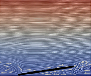
The problem to be investigated relates to the local vicinity of a body near a wall where fluid is flowing along the effectively flat wall surface, such as in a close-up view on an airfoil or in a vessel, as in figure 1. The incident velocity gradient  $\bar {\lambda }$ in the shear flow close to the wall is prescribed (where the bar notation denotes a dimensional quantity). The working below is for the steady flow around a comparatively thin, short, flat body that is located near the wall, as expressed by non-dimensional flow velocities
  $(u, v)$, corresponding Cartesian coordinates
  $(x, y)$ and pressure
  $p$. The corresponding dimensional parameters are
  $\bar {U}(u, v), \bar {L}(x, y)$ and
  $\bar {\rho } \bar {U}^2 p$ respectively, where
  $\bar {U}$ is the local representative fluid velocity taken to be
  $\bar {U} = \bar {L}$
  $\bar {\lambda }$, where
  $\bar {L}$ is the body length and
  $\bar {\rho }$ is the uniform density of the incompressible fluid. The velocity components
  $(u, v)$, pressure
  $p$ and coordinates
  $(x, y)$ are generally of order unity in the current local flow close to a wall located along the axis
  $y = 0$. The local Reynolds number is given by
  $R = \bar {U} \bar {L} /\bar {\nu } = \bar {L}^2 \bar {\lambda }/\bar {\nu }$ where
  $\bar {\nu }$ is the uniform kinematic viscosity of the fluid.
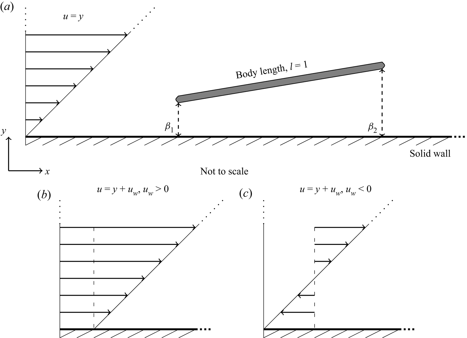
Figure 1. Sketch of the body situated near the wall within uniform shear flow parallel to the wall with the typical gap width of  $O(1)$. (a) Zero wall velocity relative to the body. (b) Positive wall velocity relative to the body. (c) Negative wall velocity relative to the body.
The body is generally translating upstream or downstream relative to the wall at a non-dimensional velocity comparable with the flow velocity  $u$ such that
  $u_w$ (the given wall velocity relative to the body) is generally of order unity. With the problem limited to what happens in the local vicinity of the body, near the wall, the flow conditions far upstream are simply those of uniform shear flow, such that
  $u = y + u_w$ and
  $v = 0$, with zero pressure, similar to those in Bhattacharyya, Mahapatra & Smith (Reference Bhattacharyya, Mahapatra and Smith2004) and related papers. The velocity of the body relative to the wall may be zero (figure 1a), positive (figure 1b), or negative (figure 1c) when measured in the streamwise direction. The body's location is fixed at a representative order-unity normal distance from the wall with the leading edge gap denoted
  $\beta _1$ and trailing edge gap
  $\beta _2$. Note that the origin is placed along the lower wall and aligns with the leading edge of the body.
The task is to solve numerically the steady incompressible non-dimensional Navier–Stokes equations about the body and between the wall and the body
 \begin{gather} \boldsymbol{\nabla} \boldsymbol{\cdot} {\boldsymbol{u}} = 0, \end{gather}
 \begin{gather}\left(\boldsymbol{u} \boldsymbol{\cdot}\boldsymbol{\nabla}\right) \boldsymbol{u} ={-}\boldsymbol{\nabla} p + \frac{\nabla^2 \boldsymbol{u}}{R}. \end{gather}
The boundary conditions are
 \begin{gather} u = u_w,\ v = 0 \quad \text{at } y = 0, \end{gather}
 \begin{gather}u = v = 0 \quad \text{at } y = f^+(x),\ f^-(x), \end{gather}
 \begin{gather}u \sim y + u_w,\ v \rightarrow 0,\ p \rightarrow 0 \text{ in the far-field}. \end{gather}
Thus (2.3) imposes the conditions of no relative slip at the wall, while (2.4) represents the no-slip requirement on the respective upper and lower surfaces  $f^+, f^-$ of the body. Here, (2.5) applies at large distances, including the incident shear effect far upstream and downstream.
The aim is to determine the velocities and pressure in the flow past and between the body and wall, in the presence of a potentially zero or non-zero wall velocity  $u(x, 0) = u_w$. Hence changes to the steady flow around the body are studied as the distance from the wall, the orientation and the Reynolds number
  $R$ are varied. As such a range of configurations for different
  $\beta _1, \beta _2$ and
  $R$ are evaluated in this paper to understand how viscous and inviscid effects close to the wall affect the developing flow structure and thus lead to nonlinearity in the flow solution with flow separation along the plate, the development of eddies in the flow, significant wake effects and upstream influence.
3. Direct numerical simulations
The direct numerical simulations were carried out in the latest release of OpenFOAM (at the time of performing the analysis version 1812) from OpenCFD Ltd. This is an open source computational fluid dynamics software that possesses a wide range of features and may be used to solve a variety of complex fluid problems. OpenFOAM's built in solver simpleFoam was used to calculate the fluid flow about the plate. This is a steady-state solver that uses the SIMPLE (semi-implicit method for pressure linked equations) algorithm to produce solutions for incompressible flows that may also include turbulence (Patankashar Reference Patankashar1980). Briefly, the SIMPLE algorithm follows a segregated solution strategy in which each of the quantities that describe the flow (the velocity, pressure and, where appropriate, variables that characterise turbulence) are solved iteratively in a sequential manner until the solution converges.
In seeking to understand how the flow structure about a single flat plate positioned near a straight wall develops, several configurations are of interest. The first quantity is the distance of the leading edge of the plate from the wall denoted  $\beta _1$ and shown in figure 1(a). The aim is to understand how the flow structure upstream, around and downstream of the plate evolves as the plate approaches impact with the wall. As such three scenarios are considered with
  $\beta _1 = 0.1, 0.05$ and
  $0.01$ respectively. The second quantity of interest is the relative wall velocity. For each of the above scenarios,
  $u_w$ may be positive, negative or zero hence three values are considered,
  $u_w = 0.1, 0$ and
  $-0.1$, to gain an initial understanding of the differences in each scenario. In later analysis in this paper larger values of
  $u_w$ are considered as prompted by the earlier results. The third parameter is the inclination of the plate relative to the wall. For each fixed
  $\beta _1$ this is defined by
  $\beta _2$ the distance of the trailing edge from the wall. Within the initial analysis presented in the next section this angle is fixed for each case such that
  $\beta _2 = 0.1 + \beta _1$. Later, plates of greater inclination are considered to understand further the effect of increased steepness on the flow characteristics. Finally, the last quantity of interest is the Reynolds number. Since locally both
  $U$ and
  $L$ are of order unity, the Reynolds number is in effect
  $R = 1/\nu$, such that the uniform kinematic viscosity of the fluid is inversely proportional to the Reynolds number and may be varied to investigate different scenarios. Here again three main scenarios have been addressed:
  $R = 10, 100$ and
  $1000$ (although because of space considerations below we mostly show results only for
  $R = 10$ and 1000).
Regarding the meshes, the left and right far fields are set ten body lengths away from the leading and trailing edge of the body, with the upper far field set five and a half body lengths away from the middle of the body. Through several iterations of the solution and varying these far-field distances, these values were found to be far enough from the body to allow the solutions and interactions to fully develop without any substantial boundary effects. The coarseness of the mesh also varied throughout the solution with the mesh refining as the body is approached (scaling by a factor of 1/100) providing greater accuracy in regions where the flow dynamics induced by the presence of the body is most significant and complex. The boundary conditions used are as follows: at the upstream edge of the domain we set  $u = y + u_w$ and
  $\partial p/ \partial x = 0$, while at the downstream edge
  $\partial u/ \partial x = 0$ and
  $p = 0$; at the upper edge
  $u = y_{max} + u_w$ with
  $\partial p/ \partial y = 0$ and at the wall
  $u = u_w$ with
  $v = 0$; on the body
  $u, v$ are zero. Here typically
  $y_{max} = 5.5 + \beta _1$, where
  $\beta _1$ is the leading edge gap between the body and the wall, and the streamwise edges were at
  $x = -10.5$ and
  $10.5$. Of note the zero gradient condition for pressure (
 $\partial p / \partial n = 0$ where
  $n$ is the normal of the wall face), zeroGradient in OpenFOAM, used here is appropriate due to the coupling of the velocity and pressure in the SIMPLE algorithm and is applied in the pressure correction step. In particular, when
  $u$ is known on the boundary, there will be no velocity correction and so the gradient of the pressure correction
  $p^\prime$ normal to the boundary must be zero (Patankar & Spalding Reference Patankar and Spalding1972). This is the standard approach when applying the SIMPLE algorithm. Note that the results presented below are post-processed to give zero pressure at the inlet for a clearer comparison of the change in pressure throughout the domain in each scenario.
The mesh resolution was also assessed prior to the full numerical study to ensure that only acceptably small mesh-related effects or inaccuracies are present in the results. To this end a quantitative comparison of results from two meshes (a finer mesh with 1 086 240 cells and a coarser mesh with 271 560 cells) for three different cases of  $U_w$, with
  $\beta _1 = 0.05$ and
  $R = 1000$, was carried out. This value of
  $\beta _1$ is the middle of the three scenarios considered later (
 $\beta _1 = 0.1, 0.05$ and
  $0.01$) and as such portrays flow characteristics seen in the two extreme cases and importantly with the diminishing wall gap. In addition,
  $R = 1000$ is the highest Reynolds number modelled in the investigation and is therefore the most computationally difficult, requiring suitably refined meshes. For
  $u_w = 0.1, 0$ and
  $-0.1$ the comparison showed errors over the entire wall pressure solution of 0.335 %, 1.33 % and 1.20 % respectively, all of which are felt to be quantitatively insignificant. Given this, we used the coarser mesh set-up due to the gain in computational time and power. The testing process provides confidence that the mesh resolution used is more than sufficient for the presented results.
In the next section results for different  $\beta _1, u_w$ and
  $R$ (as detailed above) are presented. Here, discussion focuses on how changes in these quantities affect the development of eddies in the flow, may lead to significant wake effects and can change the upstream influence of the plate. Five main aspects of the fluid flow are pertinent: the streamlines; the velocity profiles above and below the plate, upstream of the plate and in the plate's wake; and the wall pressure across the length of the domain. The results indicate how viscous and inviscid effects influence the developing flow structure as wall impact is neared.
4. Numerical results
There are many parameters of interest both for fundamental fluid dynamics and for the applications. We focus primarily on the effects of varying Reynolds number, the wall velocity and the leading edge gap with a fixed inclination. Section 4.1 discusses the numerical solutions for the streamlines followed by § 4.2 on the velocity profiles and pressures. Here the main distinct flow features are to be explored qualitatively or otherwise through the results, while specific quantitative comparisons are made in § 5 especially concerning the influence of increasing Reynolds number.
4.1. Streamlines
Considering three different scenarios, where the wall velocity is taken to be positive, zero and negative respectively, we investigate below how and when flow separation and reversal occur and eddies form about the body depending on the gap size and Reynolds number. Streamline plots about the body for  $u_w = 0.1, 0$ and
  $-0.1$ respectively, with
  $\beta _1 = 0.01$, are shown in figure 2(a–f) for
  $R = 10$ and
  $1000$. While the former case is relatively benign, by contrast the
  $R = 1000$ case is of much interest. The streamlines of the flow solutions and directional arrows for the flows help to illuminate the flow structure and give a first insight into the results.
Figure 2. Example of the fluid flow for a plate in uniform shear flow for  $\beta _1 = 0.01$, (a)
  $R = 10$ for
  $u_w = 0.1$, (b)
  $R = 1000$ for
  $u_w = 0.1$, (c)
  $R = 10$ for
  $u_w = 0.0$, (d)
  $R = 1000$ for
  $u_w = 0.0$, (e)
  $R = 10$ for
  $u_w = -0.1$, (f)
  $R = 1000$ for
  $u_w = -0.1$.
Firstly, considering  $u_w = 0.1$ in figure 2(a) (
 $R = 10$) and 2(b) (
 $R = 1000$), flow reversal is seen between the plate and wall with a clear eddy forming towards the trailing edge in the gap and becoming more significant with increased Reynolds number. In addition, the influence of the wake can be seen to develop with increased Reynolds number both downstream and under the body. The general trend for the positive wall velocity scenario is that for decreasing gap size, flow reversal becomes more likely and dominant within the underbody region. As the Reynolds number increases, for larger gaps an accelerating jet forms between the plate and the wall yet disappears as the gap closes and the mass flux is on the verge of being cut off. In addition, for larger Reynolds number the upstream influence of the plate decreases, whilst the wake effects are delayed and become more significant downstream in light of the developing eddy.
Secondly, for  $u_w = 0$ in figure 2(c) (
 $R = 10$) and 2(d) (
 $R = 1000$), an eddy develops just off the trailing edge of the body, and of a slightly larger size in the
  $R = 1000$ case. A similar trend to that of positive
  $u_w$ is seen with increased flow reversal, nonlinearity and wake effects with decreasing gap size and larger Reynolds number respectively. The main difference is that over this parameter range the effect of separation remains near the vicinity of the trailing edge, rather than throughout the gap, and does not have a significant influence upstream of it.
Thirdly, when  $u_w = -0.1$ as in figure 2(e) (
 $R = 10$) and 2(f) (
 $R = 1000$), two eddies are seen, one ahead of the body and one behind the body. Depending on the gap size the flow above and below the body behaves differently. For a larger gap, the flow beneath the plate is largely negative, with the positive flow reversing within the gap as well as ahead of the plate. When the gap decreases, the mass flux begins to be cut off, causing the flow to turn and induces a significant positive flow close to the plate. Nonlinear effects are once again significant throughout the gap region. Hence an eddy between the plate and wall forms and flow reversal now causes the negative velocity to become positive beneath the plate. As the Reynolds number increases the length scale of the upstream effect reduces whilst that of the wake effect increases.
4.2. Velocity profiles and pressures
Studied here are three different scenarios in which the leading edge gap is varied ( $\beta _1 = 0.1, 0.05, 0.01$) with a fixed relative trailing edge gap (
 $\beta _2 = \beta _1 + 0.1$). For each case the wall velocity and Reynolds number are varied,
  $u_w = 0.1, 0, -0.1$ and
  $R = 10, 100, 1000$. Plots for
  $R = 100$ are not shown.
To begin, the underbody velocity profiles are considered with the results presented in figures 3–5. In figure 3, where the wall velocity  $u_w = 0.1$, for the largest gap width
  $\beta _1 = 0.1$ (top row of results), as the Reynolds number increases the velocity in the gap under the body also increases. The fluid undergoes an acceleration as it is squeezed between the plate and the wall forming an accelerating jet. At the trailing edge this effect diminishes as the developing wake begins to interact with the fluid flow in the gap. Above the body the velocity profiles tend towards the outer linear velocity with increasing
  $y$, which is seen in all cases for figures 3–5. As the gap decreases, the fluid continues to undergo an acceleration under the body close to the leading edge, but this becomes less pronounced throughout the rest of the underbody region. For
  $\beta _1 = 0.05$ the developing wake has a greater influence near the leading edge, especially for the lower Reynolds number, with greater potential for flow reversal seen close to the trailing edge. As
  $\beta _1$ decreases further the closing of the gap begins to cut off the mass flux beneath the body, inducing flow reversal there. For each value of
  $R$, the onset of flow separation occurs close to the leading edge, around
  $x = 0.06$, and fills the entire region under the body. This indicates that a considerable eddy is forming between the plate and the wall. As would be expected, the results here and in the rest of the present section are consistent with the streamline plots of the previous section.
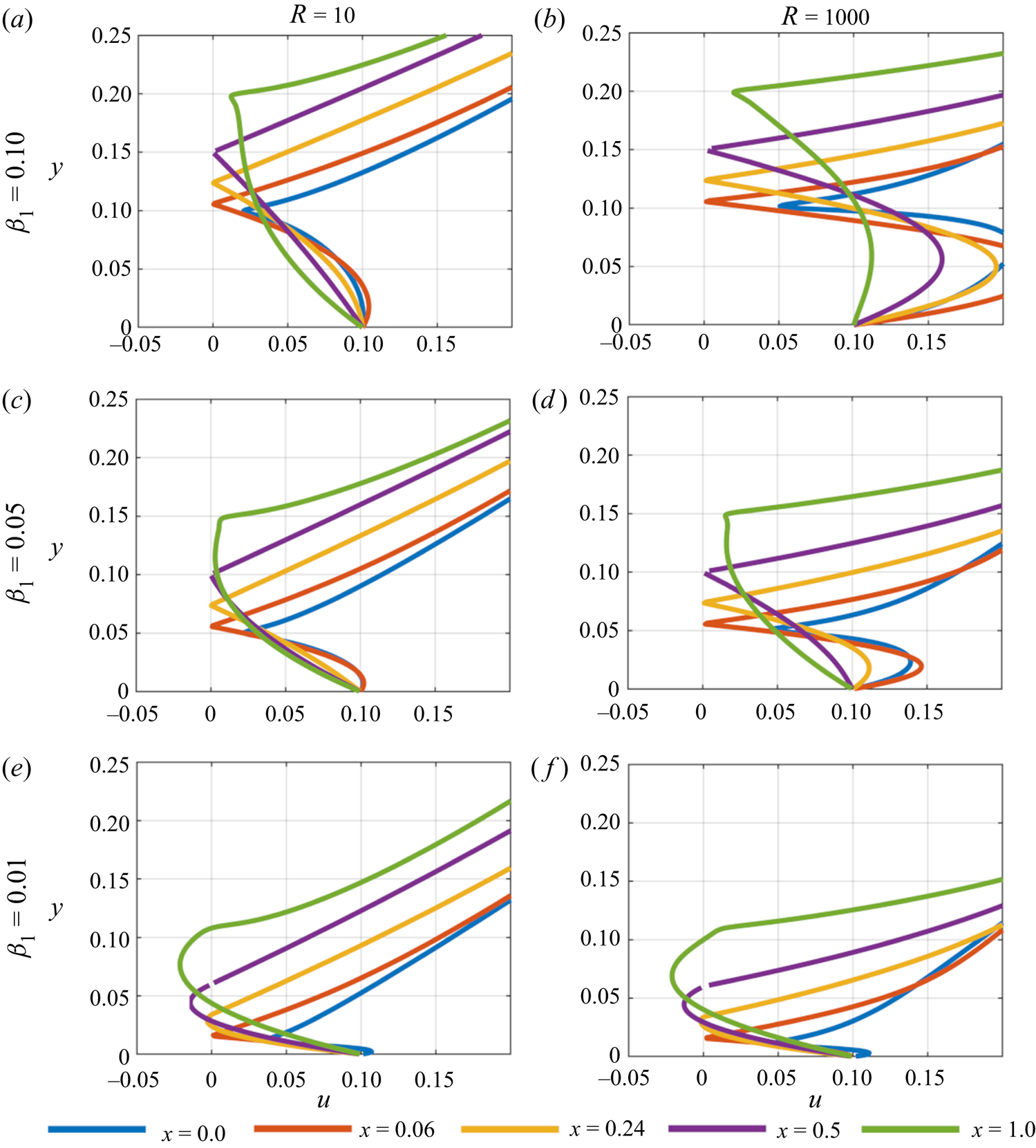
Figure 3. Velocity profiles underneath and on top of the plate taken at various points for  $u_w = 0.1$. Flow reversal is seen along the plate as the leading edge gap,
  $\beta _1$, decreases.
Similar trends are seen in figure 4 for  $u_w = 0$; however, flow reversal is now seen in the
  $\beta _1 = 0.1$ case when the Reynolds number is low. In each case with flow reversal in figure 4, separation occurs closer to the trailing edge and does not extend as far into the underbody gap. Hence owing to the lower velocities under the body, the developing wake has a greater influence on the flow structure near the trailing edge.
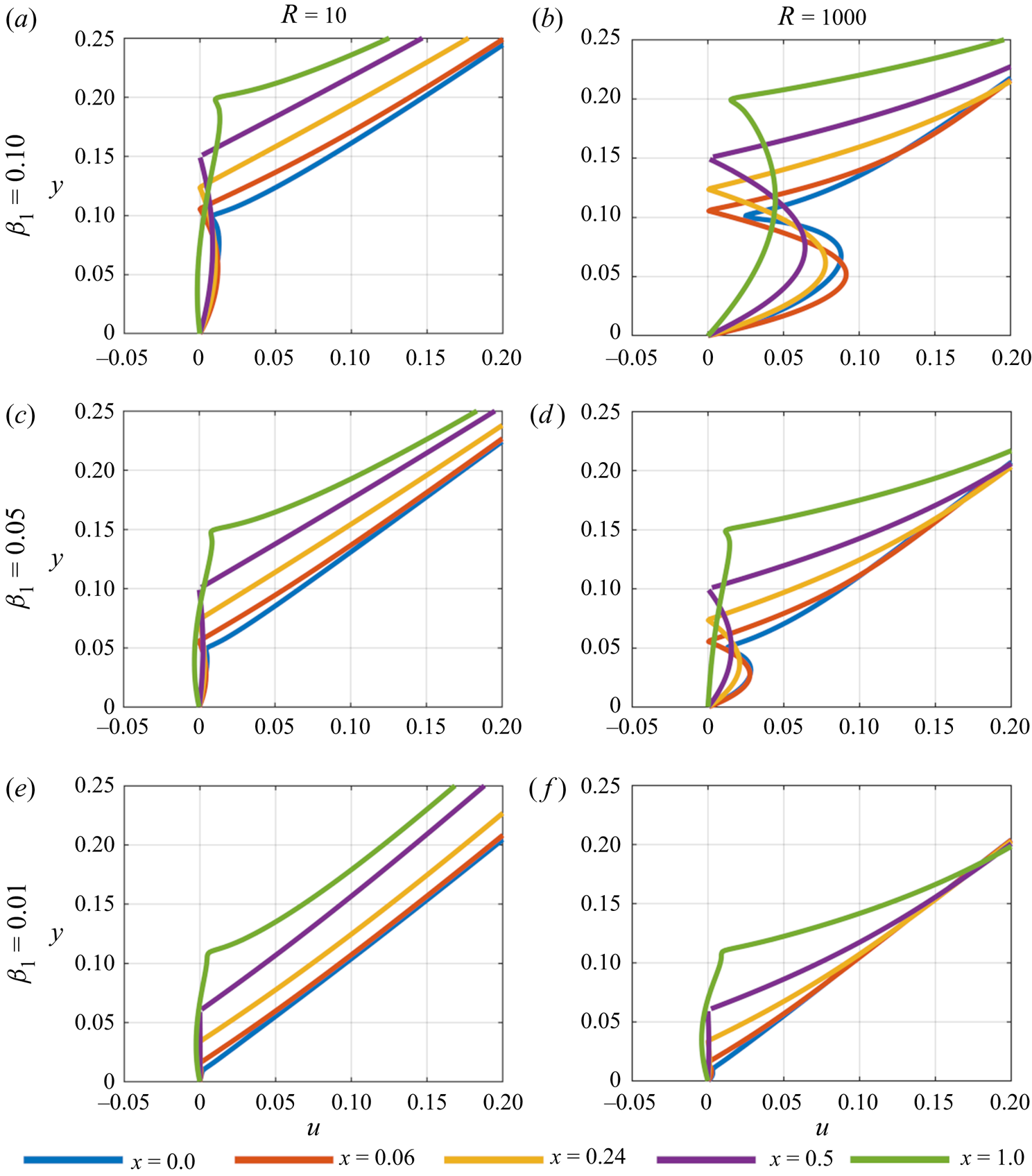
Figure 4. Velocity profiles underneath and on top of the plate taken at various points for  $u_w = 0$. An eddy forms on the wall as the leading edge gap,
  $\beta _1$, becomes smaller.
For wall velocity  $u_w = -0.1$ the velocity profiles in figure 5 are markedly different. To understand when flow reversal occurs in these scenarios we note that the far-field velocity has
  $u \leq 0$ for
  $y \leq 0.1$ and
  $u > 0$ for
  $y > 0.1$. Starting with
  $\beta _1 = 0.1$ and
  $R = 10$, the body is stationed at the cusp of the change in velocity direction,
  $y = 0.1$. Flow separation is shown from the
  $x = 0.24$ station onwards under the body, with the velocity remaining negative for values of
  $y > 0.1$ in the underbody gap to the trailing edge. As
  $R$ increases, separation persists, but it is less prominent towards the body's leading edge, moving closer towards the trailing edge. For
  $\beta _1 = 0.05$ and
  $R = 10$, flow reversal has reduced within the majority of the underbody gap. Above the body towards the leading edge, however, the velocity has become positive for
  $y < 0.1$ indicating a reversal in the flow ahead of the body. The mass flux is again beginning to be cut off under the body as the gap reduces such that the flow is squeezed through the small gap, and hence an eddy begins to form (the precise nature of which will be clearer in the subsequent upstream analysis). Examining the underbody velocity at
  $x = 0.9$ (not included) marginal reversal of the flow is seen close to the underside of the body indicating that an eddy is forming off the trailing edge. This is due to the negative flow under the body undergoing a reversal as it interacts with the developing wake (this will become clearer in the later wake analysis). Overall, as
  $R$ increases there is a marginal change in the velocity values, but the previously described trends prevail. For
  $\beta _1 = 0.01$, separation is more significant under the body as the gap closes off the mass flux further with positive velocity values occurring around
  $x = 0.5$. The reasons are as above, with the closing gap turning the flow back along the plate. Given the location of the reversal near the trailing edge and close to the plate an eddy is forming in the wake. An eddy is also seen developing ahead of the leading edge with
  $u > 0$ for
  $y < 0.1$.
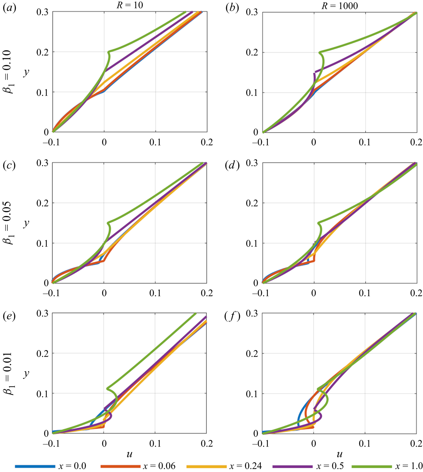
Figure 5. Velocity profiles underneath and on top of the plate taken at various points for  $u_w = -0.1$. Flow reversal becomes more prominent further along the body as the leading edge gap,
  $\beta _1$, decreases. An eddy is also forming ahead of the leading edge in most cases.
Figures 6–8 present the upstream influence of the body on the fluid for  $u_w = 0.1, 0$ and
  $-0.1$ respectively. From figure 6, for
  $\beta _1 = 0.1$ and
  $u_w = 0.1$, the fluid underneath the body (
 $y < 0.1$) undergoes a mild acceleration close to the wall at each
  $x$ station before decelerating as the underside of the plate is approached. Above the plate the fluid accelerates to the far-field velocity as the distance from the plate increases. With larger Reynolds number the profiles further upstream become more linear indicating a reduced upstream influence, whilst the acceleration of the fluid in the leading edge region is amplified as the leading edge is approached. When
  $\beta _1$ is decreased similar behaviour is seen, although the amplitude of the plate's upstream influence further reduces. For
  $\beta _1 = 0.01$ the acceleration below the leading edge is no longer seen which is expected due to the closing gap. The velocity profiles now more closely resemble those of the far field.
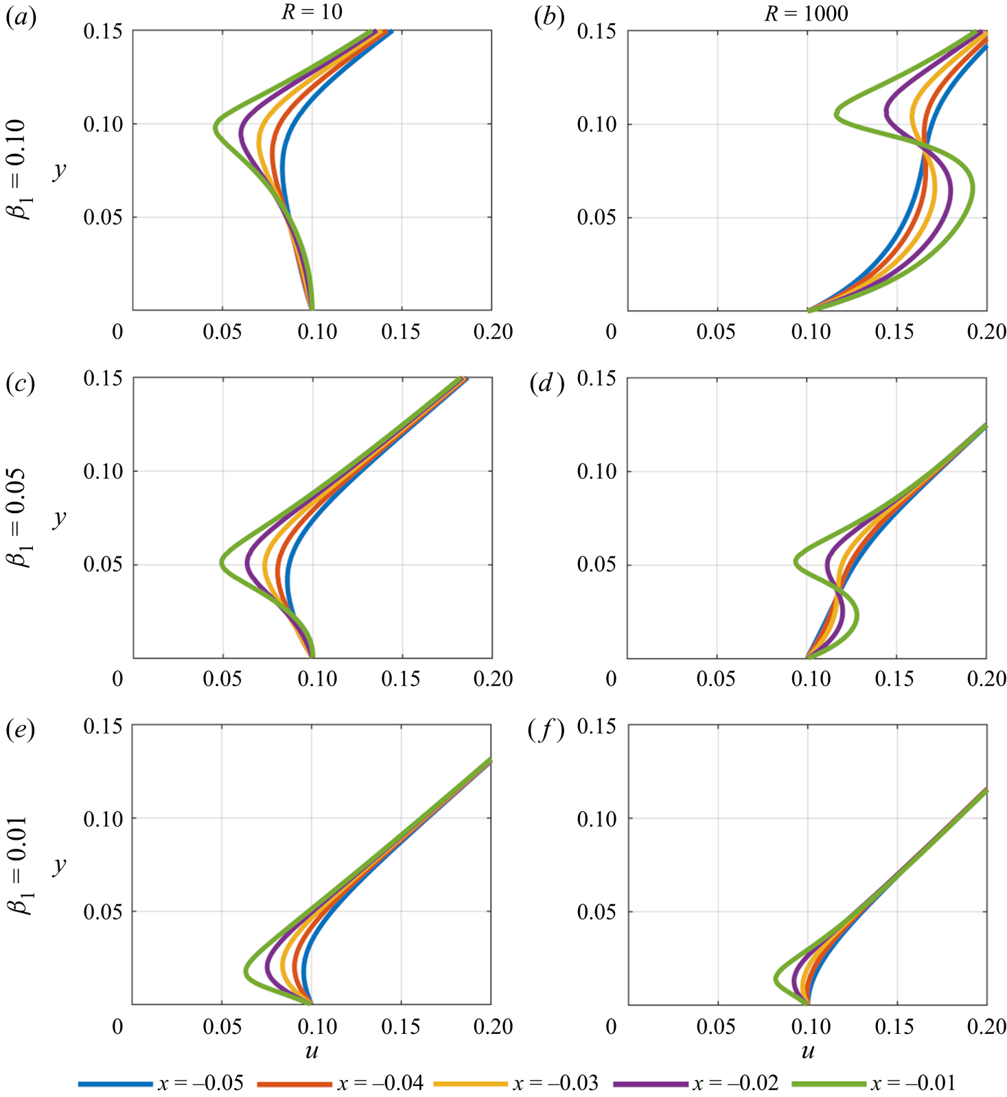
Figure 6. Velocity profiles upstream of the plate's leading edge for  $u_w = 0.1$.
In figure 7 a similar dynamics is seen with the upstream influence again reducing with Reynolds number and gap size. Interestingly for decreasing  $\beta _1$ the upstream influence is far less significant in this scenario even close to the body. For
  $\beta _1 = 0.01$ the velocity profiles again closely resemble the shear flow of the far field.
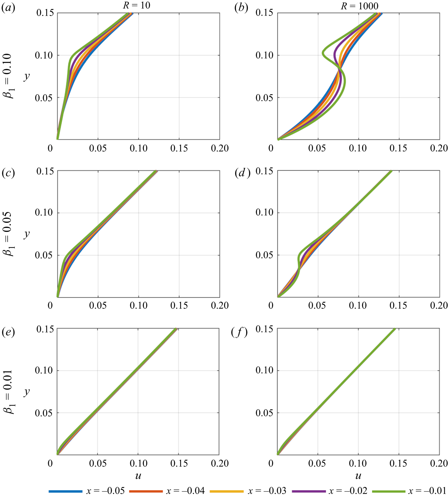
Figure 7. Velocity profiles upstream of the plate's leading edge for  $u_w = 0$.
When the wall velocity  $u_w = -0.1$, in figure 8, there is an initial, mild upstream influence from the body for the largest gap size which again diminishes with larger
  $R$. In contrast to the previous scenarios, decreasing the gap width leads to increased upstream influence. For
 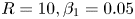 $R = 10, \beta _1 = 0.05$ flow reversal is seen around
  $y = 0.08$ with the effects felt further upstream. This continues to be seen for marginally larger
  $y$ values as
  $R$ increases indicating the trend towards reduced upstream influence with
  $R$. Finally, with
  $\beta _1 = 0.01$ the flow reversal is more pronounced upstream of the leading edge. The above results corroborate the observations from the relevant underbody profiles with an eddy forming ahead of and above the plate's leading edge.
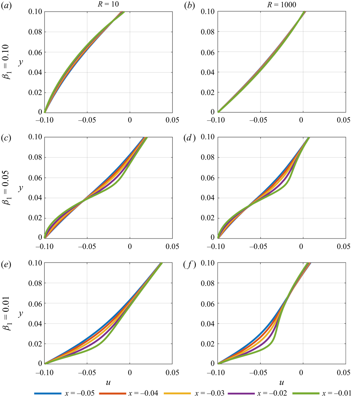
Figure 8. Velocity profiles upstream of the plate's leading edge for  $u_w = -0.1$.
Presented in figures 9–11 are the wake developments for each case. For figure 9, overall whilst  $R$ increases the extent of the downstream wake effect also increases. When the gap between the plate and the wall is large, there is greater variation in the velocity profiles for lower
  $R$. Having undergone a deceleration below the plate, the flow begins to accelerate back towards the far-field shear flow. However, for larger
  $R$ values this acceleration is markedly less such that the wake and its effects persist further downstream of the trailing edge (as shown by the bunching of the velocity profiles). At the highest
  $R$ studied the jet effect and the acceleration of the fluid (shown in figure 3) now continue through to the trailing edge, and so the wake development is delayed further downstream. As the gap size decreases, this trend in enhanced wake effects continues with the downstream velocity profiles showing decreasing variation with increasing
  $R$. Hence, for
  $\beta _1 = 0.01$ where separation occurs below the plate and flow reversal is significant, flow reversal dominates in the wake far beyond the trailing edge. Decreasing wall gap leads to significant wake effects and eddies forming under and beyond the plate, with effects beginning close to the trailing edge and penetrating further downstream with increased
  $R$. Since the flow reversal occurs in the middle of the gap an eddy sits between the plate and wall. Of further interest, in each scenario, as the
  $x$ distance from the trailing edge increases the velocity profiles satisfactorily approach the far-field ones as expected.
Figure 9. Velocity profiles of the plate's wake for  $u_w = 0.1$.
In figure 10, where  $u_w = 0$, the same trend is seen in each case; however, separation is seen when
  $\beta _1 = 0.1$ as well, close to the trailing edge of the plate. Interestingly, here the
  $y$ values indicate that the eddy is forming along the wall. In addition, from the cases where
  $\beta _1 = 0.05$ and
  $\beta _1 = 0.01$, as
  $R$ is increased the eddy moves further along the wall, away from the body, due to the accelerating fluid jet between the plate and the wall delaying the onset of the wake. So again, with a decreasing gap, flow reversal dominates the wake, having a greater effect with higher
  $R$. Further downstream of the trailing edge the velocity profiles approach the far-field ones for each value of
  $R$ and
  $\beta _1$.
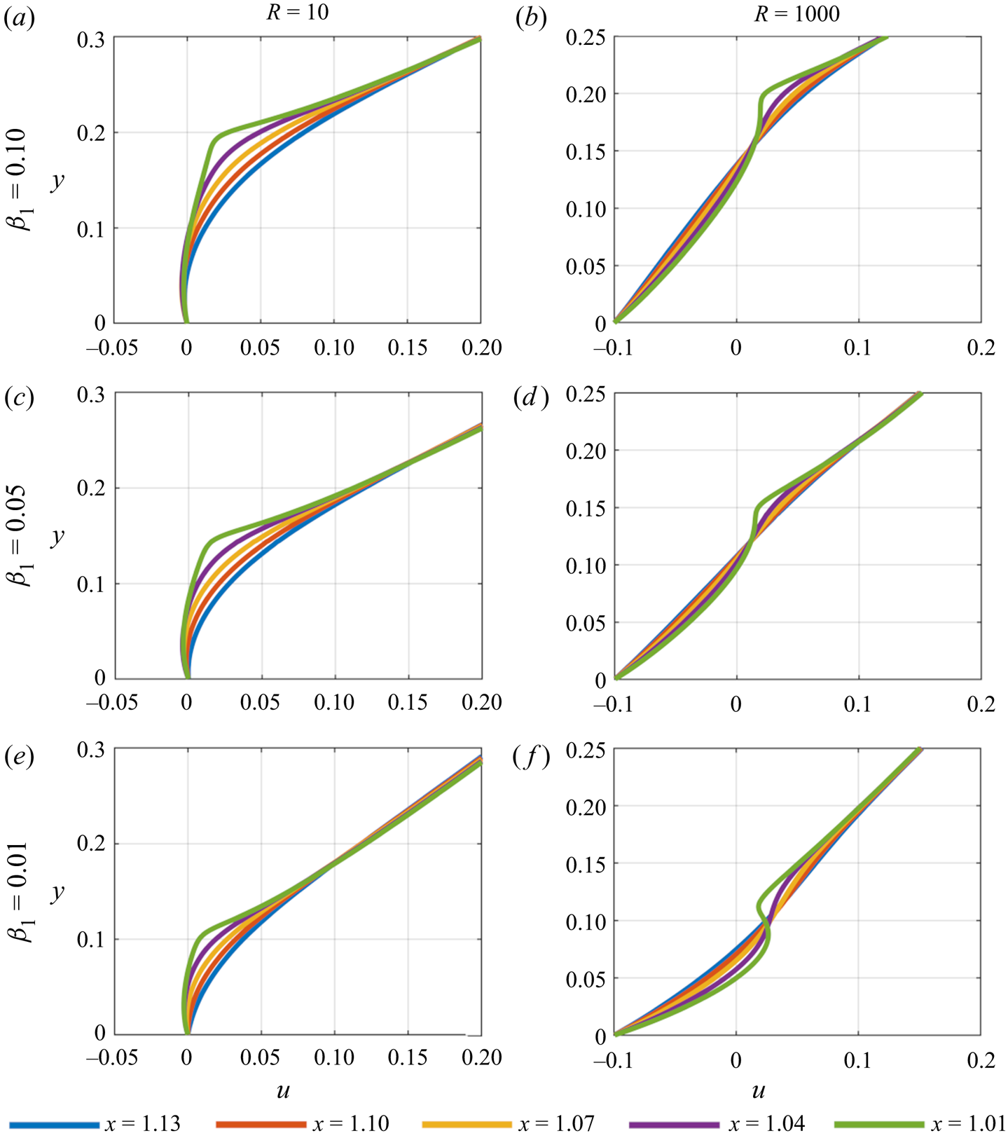
Figure 10. Velocity profiles of the plate's wake for  $u_w = 0$.
Whilst a similar trend continues in figure 11 where  $u_w = -0.1$, there are several notable differences depending on the size of
  $\beta _1$. Firstly, in the cases where
  $\beta _1 = 0.1$, we see that
  $u <0$ for
  $y > 0.1$ beneath the plate. Here, the dynamics noted for figure 5 is seen to persist into the wake, with flow reversal occurring further downstream with increasing
  $R$ and being present further into the wake. This helps to confirm the earlier observation that an eddy is forming off the trailing edge as the flow under the body interacts with the developing wake. The presence of this developed wake eddy leads to the flow beneath the body becoming almost wholly negative (reversed). Secondly, however, as the body is placed closer to the wall, the flow reversal near the leading edge (previously noted due to the closing of the mass flux) also persists into the wake. As before, in each scenario the velocity profiles approach the far-field ones further downstream.
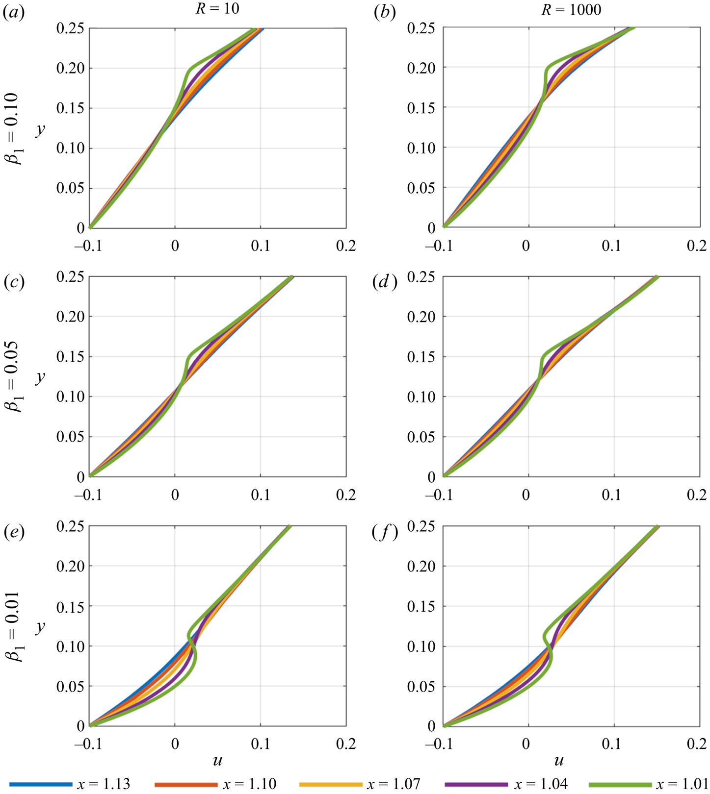
Figure 11. Velocity profiles of the plate's wake for  $u_w = -0.1$.
Plots for the wall pressure across the length of the domain and on top of the body are presented in figures 12–14. Beginning with the case for  $u_w = 0.1$, figure 12(a), several features stand out for increasing
  $R$. Initially, a quite localised jump in pressure is seen clearly in line with the leading edge of the plate for
  $R = 10$, which then diminishes as
  $R$ increases. In addition the magnitude of wall pressure decreases with
  $R$ as expected. Concerning flow separation the magnitude and sign of the pressure gradient are important. In each of the
  $\beta _1 = 0.1$ cases, a favourable pressure gradient persists under the body. An adverse pressure gradient continues into the wake but in these cases the slope is not too steep. As
  $\beta _1$ decreases, however, the pressure minimum moves towards the leading edge of the plate, creating a sharper shorter region of favourable pressure gradient and introducing a significant adverse pressure gradient under the body which becomes more pronounced with decreasing
  $\beta _1$. The trend in the development of the adverse pressure gradient beneath the body with
  $R$ and
  $\beta _1$ confirms the above observations regarding when and where flow separation occurs beneath the body and the increased flow reversal within the wake.
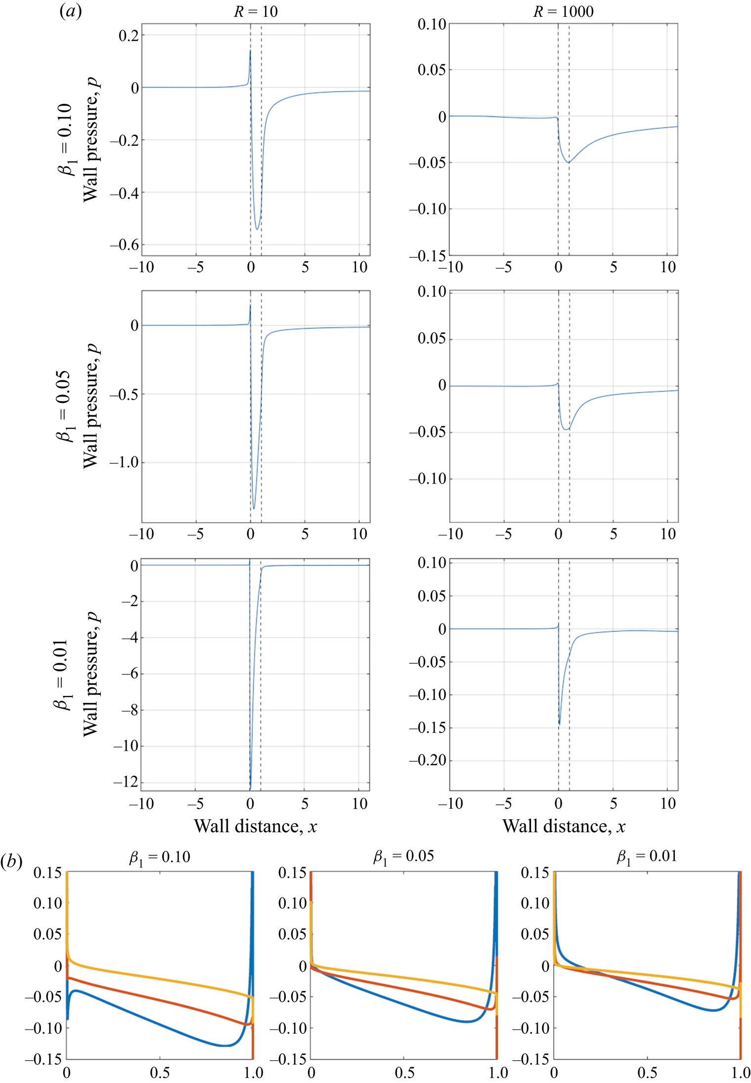
Figure 12. Plot of pressure for  $u_w = 0.1$, (a) along the length of the lower wall, (b) along the upper surface of the body, blue:
  $R = 10$, red:
  $R = 100$, yellow:
  $R = 1000$.
Regarding overbody pressure for  $u_w = 0.1$, figure 12(b), as the wall gap reduces the magnitude of the pressure also reduces. In addition, for increasing Reynolds number the pressure reduces further across the length of the body tending towards zero. Notably, the values seen here are typically an order of magnitude less than the below wall pressure as expected.
Figure 13(a), where  $u_w = 0$, displays the same trend for varying
  $R$ and
  $\beta _1$. However, now the favourable pressure gradient is seen over the majority of the body for decreasing
  $\beta _1$, yet with an increasingly steep adverse gradient near the trailing edge and in the wake. This corroborates the observations above. Regarding overbody pressure for
  $u_w = 0.0$, figure 13(b), the same trends of reduced wall gap leading to reduced overbody pressure and increased Reynolds number reducing the pressure further across the body are seen. The values are again an order of magnitude less than the below wall pressure.
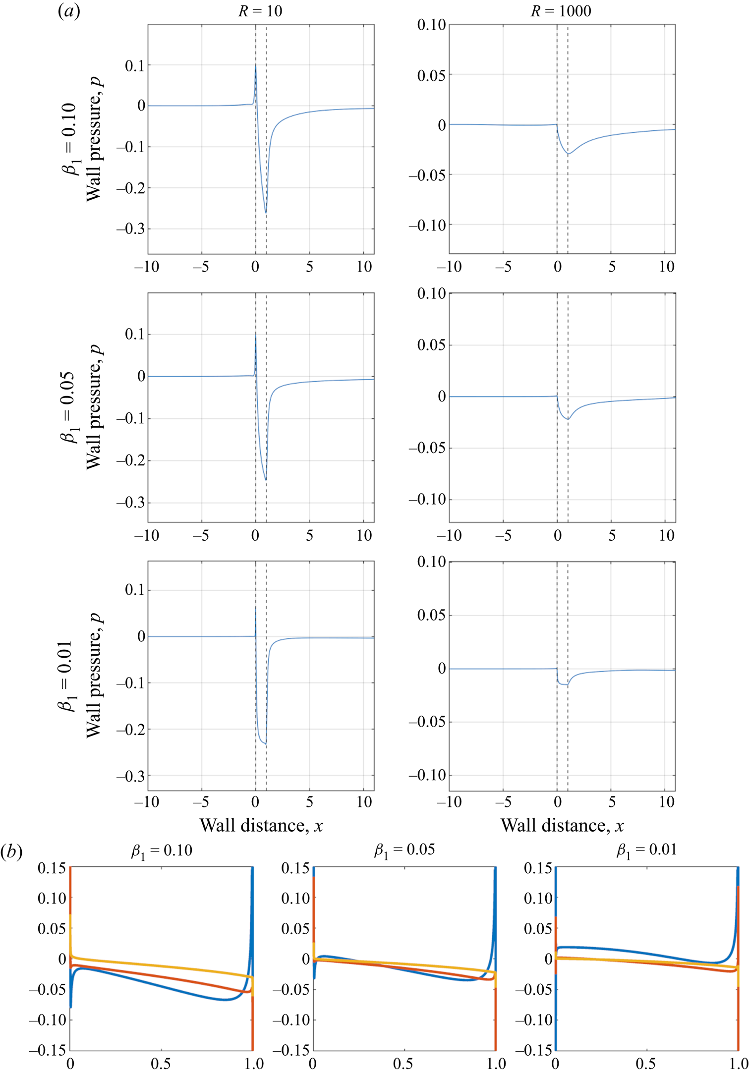
Figure 13. Plot of pressure for  $u_w = 0.0$, (a) along the length of the lower wall, (b) along the upper surface of the body, blue:
  $R = 10$, red:
  $R = 100$, yellow:
  $R = 1000$.
Finally in figure 14(a), where  $u_w = -0.1$, the trends seen in flow separation and reversal are reflected in the behaviour of the wall pressure for increasing
  $R$ and decreasing
  $\beta _1$. For
  $\beta _1 = 0.1$, the pressure is favourable under most of the body whereas in the wake (
 $x \geq 1$) a significant adverse gradient is introduced. With increasing
  $R$, the gradients remain largely favourable in
  $x$ beneath the extent of the body. For
  $\beta _1 = 0.05$ and
  $\beta _1 = 0.01$, similar trends to figures 12 and 13 are seen in that there is a strong adverse gradient just after the leading edge but a significant favourable gradient below the majority of the body. Ahead of the body (
 $x \leq 0$) there are also small gradients, in the region of flow reversal there, a finding which agrees with the upstream dynamics and flow reversal seen ahead of the body in figure 8 as discussed earlier in this section. In figure 14(b),
  $u_w = -0.1$, the upperbody pressure is very small indeed, remaining relatively close to zero for all cases.

Figure 14. Plot of pressure for  $u_w = -0.1$, (a) along the length of the lower wall, (b) along the upper surface of the body, blue:
  $R = 10$, red:
  $R = 100$, yellow:
  $R = 1000$.
5. Further properties
The additional features requiring consideration here are the lift, drag and moment exerted on the given body, as described in § 5.1 below, and the effects of varying the body inclination and the velocity of the wall as well as details of the dependence on Reynolds number which are explored in § 5.2 below.
5.1. Lift, drag and moment
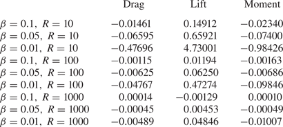
Tables 1–3 show the results for the lift, drag and moment on the body. These are of basic fluid-dynamical concern as well as application. In the three  $u_w$ cases, the sizes of the drag, lift and moment values increase with the smaller wall gap, and reduce with larger Reynolds number as expected (though this trend is less pronounced in the
  $u_w = 0$ case). Of particular interest, the lift is an order of magnitude larger than the drag in each run across each of the three cases, which is in line with the relevant asymptotic analysis in Palmer & Smith (Reference Palmer and Smith2020).
Table 1. Drag, lift and moment acting on the body for  $u_w = 0.1$ with varying wall gap and local Reynolds number.
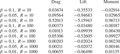
Table 2. Drag, lift and moment acting on the body for  $u_w = 0.0$ with varying wall gap and local Reynolds number.
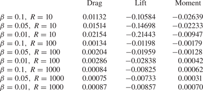
Table 3. Drag, lift and moment acting on the body for  $u_w = -0.1$ with varying wall gap and local Reynolds number.
5.2. Varying inclination; increasing wall velocity; influences of Reynolds number
Taking the preceding results together, three outstanding questions now need investigating further. Throughout the paper the trailing edge gap has been defined as  $\beta _2 = \beta _1 + 0.1$; however, given the significant effect that the leading edge gap has on flow reversal it is worthwhile investigating how the size of
  $\beta _2$ influences the fluid flow. Figure 15 presents the wall pressure for
  $u_w = 0.1$ with
  $\beta _1 = 0.01$ and
  $R = 1000$, but now with three different trailing edge gaps,
  $\beta _2 = 0.11, 0.21$ and
  $0.31$, where
  $\beta _2 = 0.11$ is the same as the previous case for reference. As the body increases in pitch, the adverse pressure gradient that is seen to cover the whole body and wake for the
  $\beta _2 = 0.11$ case begins to extend further downstream. The severe slope that existed for a shorter distance towards the leading edge now becomes less steep downstream of the body's midpoint but the adverse gradient continues into the wake. As expected, increasing inclination leads to flow separation under the body and further downstream.
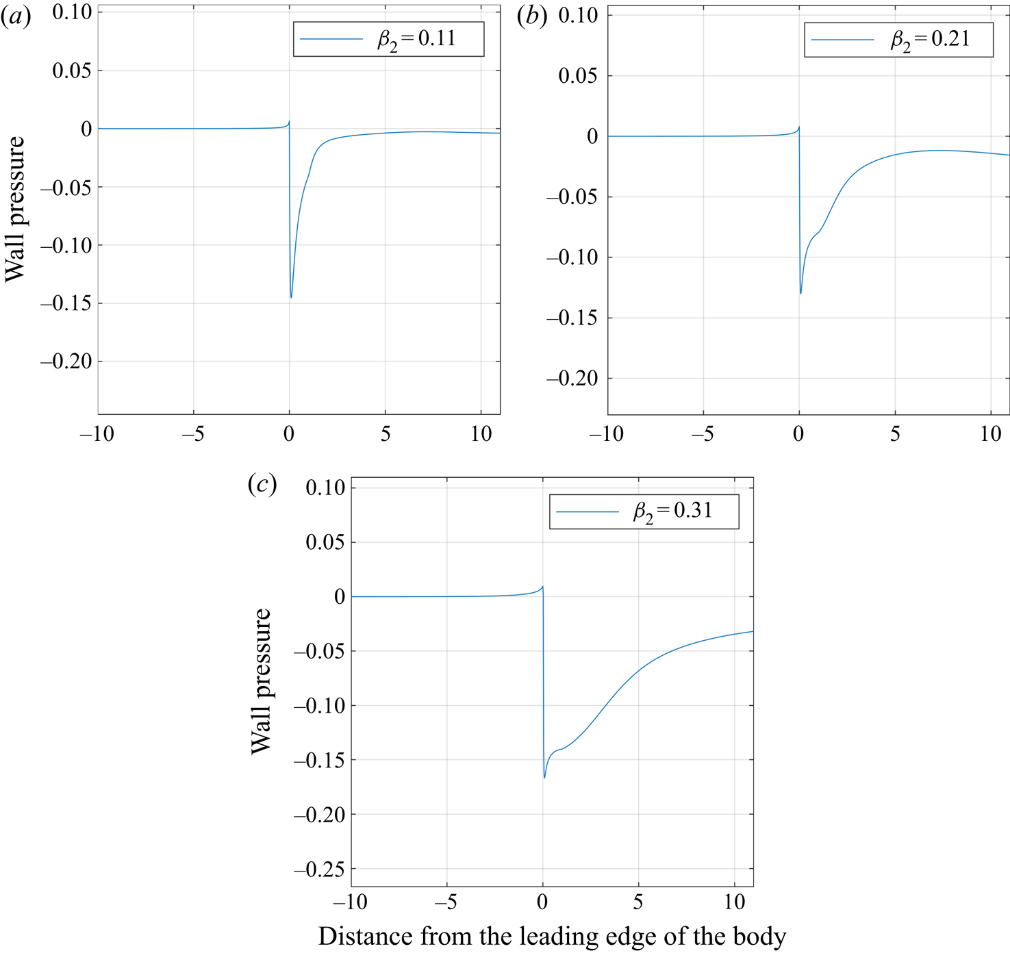
Figure 15. Wall pressure for  $R = 1000$ with
  $\beta _1 = 0.01$ and
  $\beta _2 = 0.11, 0.21$ and
  $0.31$. With increased
  $\beta _2$, relative to fixed
  $\beta _1$, the adverse pressure gradients cover a larger region under the body and into the wake.
Next, given the difference in the form of the fluid flow and dynamics seen for the different wall velocities, larger values of  $u_w$ are now considered to understand how the interaction changes. In figure 16 the wall pressures are shown for the case where
 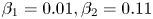 $\beta _1 = 0.01, \beta _2 = 0.11$ and
  $R = 1000$ with
  $u_w = 0.2$ and
  $-0.2$. Compared to the previous results figures 12 and 14 it is seen that in both cases the magnitude of the wall pressure has doubled yet the region over the body and wake for which the pressure varies has remained the same (
 $x$-distance along the wall). Thus, the pressure gradient across the body and in the wake for both scenarios has become increasingly adverse indicating the flow reversal is more likely to occur with greater influence, inducing larger changes in flow velocities and directions. This trend in the results agrees with the findings of the asymptotic theory in Jones & Smith (Reference Jones and Smith2003) which apply for negligible incident shear.
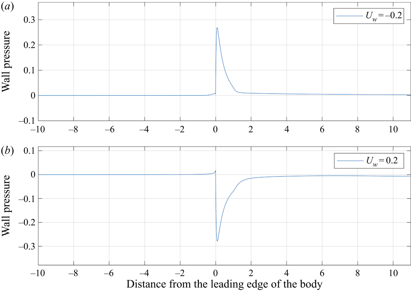
Figure 16. Wall pressure for  $R = 1000$ with
  $u_w = 0.2$ and
  $-0.2$. With increased
  $u_w$ there are larger adverse pressure gradients under the body and in the wake.
Finally, concerning scales with respect to increasing Reynolds numbers, from figures 12, 13 and 14 it is observed that the magnitude of wall pressure falls with increasing Reynolds number. In fact, given the set-up and definition of the fluid quantities we anticipate that a distinguished scaling exists between the Reynolds number and the order of magnitude for the wall pressure. This can be readily seen. From the modelled problem, the components of (2.2) to leading order suggest that  $uu_x \sim (1/R) u_{yy}$. Given the expectation that
  $U = O(y)$ and that
  $x = O(1)$ is known, we thus require
  $y \sim R^{-1/3}$. Furthermore, for (2.2) to balance we have that
 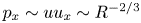 $p_x \sim uu_x \sim R^{-2/3}$. Hence, we anticipate that given these scalings, for
  $\beta _1 = R^{-1/3}, \beta _2 = 2 \times R^{-1/3}$ and
  $u_w = R^{-1/3}$, the wall pressure response should be
  $O(R^{-2/3})$. Presented in figure 17 are five such scenarios where
  $R = 10, 50, 100, 500$ and
  $1000$. Of note, in each case the magnitude of wall pressure is falling with
  $R$, such that in comparison to
  $R^{-2/3}$ the scaling holds quantitatively to within a multiplicative constant in each case: see table 4.
Figure 17. Wall pressure for  $\beta _1 = R^{-1/3}, \beta _2 = 2 \times R^{-1/3}$ and
  $u_w = R^{-1/3}$ with
  $R = 10, 50, 100, 500$ and
  $1000$. In each case the magnitude of the wall pressure is of the order
  $R^{-2/3}$, indicating (see also table 4) that a distinguished scaling exists between wall pressure and Reynolds number.
6. Conclusion
The major aims of this study have centred on understanding the influence that a thin inclined body has on the fluid motion when placed within a uniform near-wall shear flow. In particular, the effect of distance between the body and the wall has been of chief concern in order to appreciate how the flow structure changes about the body as impact is neared. The investigations conducted here have considered how the gap size, the wall speed and Reynolds number each affect the flow solution and lead to nonlinearity and accompanying flow separations within the fluid flow. Our interest has been in a fixed body in a steady-state flow. The occurrences of significant flow reversal beneath the body (for positive wall velocity), off the trailing edge (for zero wall velocity) and ahead of the body (for negative wall velocity) as impact is neared are most notable. There is also much dependence on the streamwise translation of the body and on the Reynolds number, particularly for flow within the upstream and wake regions. Recent work in Palmer & Smith (Reference Palmer and Smith2020) describes an asymptotic investigation of body-motion effects. In summary, the latter work applies to a thin body moving in the lower reaches of a boundary layer or channel flow at high Reynolds number with the interaction then becoming centred in the viscous–inviscid layer near the wall where the  $1/3$ scalings, discussed at the end of § 5, hold in all such cases. The governing system there comprises the nonlinear interactive boundary layer equations subject to wall and body-surface conditions as in the present paper in effect but with important short scale upstream influence arising in an Euler region surrounding the leading edge of the body and with a Kutta condition at the trailing edge. These flow properties are coupled with the mass-acceleration equations of the body movement forced by the flow pressure acting at the body surface, thereby yielding a dynamic interaction between the fluid and body motions. Of most relevance here are the significant regions of flow reversal encountered and the nonlinear dynamics of viscous–inviscid unsteady fluid motions, especially with regard to unusual flow structures during impacts upon the wall, combined with the quantitative comparison of table 4 and § 5.2.
Addressing numerical solutions of the Navier–Stokes equations for a nonlinear fluid–body interaction over a range of moderate Reynolds numbers and also comparing qualitatively and quantitatively (as above) with analysis for high Reynolds numbers have been novel facets of the current paper. This fills a gap in knowledge in the sense that there has been little work done previously on the effects of increasing inertia, of the gap width between a body and the wall and of the body inclination. Substantial flow separation has been found to occur on the body surface and at the wall as suggested in asymptotic theory along with higher pressure variations on top of the body when the gap width is increased (Palmer & Smith Reference Palmer and Smith2019, Reference Palmer and Smith2020). With increased local Reynolds numbers enhanced wake responses have been found, together with greatly condensed upstream influence near the leading edge, increased sensitivity to body orientation, pressure dominance in the total lift and moment on the body, new insight into the complex flow structure developing and quantitative agreement with recent viscous–inviscid interaction analysis, as mentioned earlier concerning scales.
Connections, however remote, exist with the original applications mentioned in the Introduction. These are principally for the movement of ice crystals, for example near the solid surface of a transport vehicle, and in terms of increased physical understanding to improve models used in industry. Additional connections exist with the scientific problems or issues also mentioned in the Introduction, for example: through the question of attraction or repulsion of a body near a solid surface in the presence of inertial influences at moderate Reynolds numbers, for which the current work confirms that either response is possible depending on the specific positioning of the body; and through increased appreciation of the dominant physical scales and parametric effects acting at moderate flow rates.
Following the current work there are many other issues that would benefit from future study. To start, a wider range of body shapes need investigating. In particular, the body shape and the initial conditions of the body position will affect whether leading edge, trailing edge or mid-chord locations are closest to the wall as impact is neared. This is important since shapes are varied in reality and thus more details of trailing edge and mid-chord impacts are required, in particular concerning trailing edge separations and upstream influence (Smith Reference Smith1984; Jones & Smith Reference Jones and Smith2003). The development of the fluid flow about the body and the potential nonlinearity of the flow are expected to be changed by these additional features. In addition future developments in understanding would benefit from three-dimensional analysis, as well as the inclusion of unsteady flows and multiple bodies; the current work on two-dimensional flow acts rather as a reasonable first model whereas three-dimensional interactions have still to be considered seriously.
Table 4. Scaling results for magnitude of wall pressure compared to  $R^{-2/3}$ for
  $R = 10, 50, 100, 500$ and
  $1000$, with
 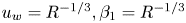 $u_w = R^{-1/3}, \beta _1 = R^{-1/3}$ and
 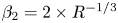 $\beta _2 = 2 \times R^{-1/3}$. The magnitude of wall pressure is seen to be within a multiplicative constant of
  $R^{-2/3}$, hence the wall pressure appears to be
  $O(R^{-2/3})$ as expected.
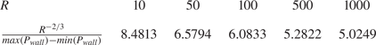
Acknowledgements
Thanks are due to personnel at AeroTex (R. Moser, I. Roberts, C. Hatch) for their interest in the area, to EPSRC through grants EP/R511638/1, GR/T11364/01, EP/G501831/1, EP/H501665/1, EP/K032208/1 during part of this research, to EPSRC /IAA and AeroTex for support of R.A.P., and to A. Rothmayer for helpful discussion of a number of related points. We are grateful also to the referees for their constructive comments.
Funding
This work was supported by EPSRC (grant number EP/R511638/1) with matched funding and support from AeroTex UK LLP.
Declaration of interests
The authors report no conflict of interest.
Author contributions
R.A.P. performed the simulations. All authors contributed equally to analysing data and reaching conclusions, and in writing the paper.


