2.1. Definition of the S(C) effect

The definition of the S(C) effect is given by applying a decomposition formula. The formula was proposed to investigate the influence of nonlinear waves (Li et al. Reference Li, Tian, He and Zhang2021) and convergent geometry (Ge et al. Reference Ge, Zhang, Li and Tian2020) on the evolution of RM instability. For completeness, we give a brief derivation of the S(C) effect.

The mixing width is defined as the distance from the bubble-zone front to the spike-zone front, i.e.

(2.1a)\begin{equation} W\equiv {\rm sgn}(A)\,(R_{B}-R_{S}), \end{equation}

and hence

(2.1b)\begin{equation} \dot{W}= {\rm sgn}(A)\,(\dot{R}_{B}-\dot{R}_{S}), \end{equation}

where the overdot means the time derivative, $A=(\rho _{out}-\rho _{in})/(\rho _{out}+\rho _{in})$ is the Atwood number, $R_{B}$ is the radius where the Favre-averaged light-fluid mass fraction profile in the streamwise direction $\tilde {Y}_{l}(R_{B},t)=0.01$, and $R_{S}$ is the radius where $\tilde {Y}_{l}(R_{S},t)=0.99$.

For a physical variable $f$, $\bar {f}$ and $\tilde {f}$ represent the Reynolds-averaged streamwise-direction profile and the Favre-averaged streamwise-direction profile, respectively. Here, $\tilde {f}=\bar {\rho f}/\bar {\rho }$, where $\rho$ is the fluid density. Correspondingly, $f^{\prime }=f-\bar {f}$ and $f^{\prime \prime }=f-\tilde {f}$ are the fluctuating parts of the variable. The averaged velocity is aligned in the streamwise direction. For consistency, in the planar geometry, we use $r$ to indicate the streamwise direction.

For the Favre-averaged mass fraction profile $\tilde {Y}(r,t)$, where $r$ is the streamwise direction, at any given time $t$, the function of space $\tilde {Y}(r,t)$ is monotonic when $\tilde {Y}\in ( 0,1)$. Therefore, the inverse function of $\tilde {Y}(r,t)$ can be defined as $R_{\tilde {Y}}(Y,t)=\tilde {Y}^{-1}(r,t)$ ($Y\in ( 0,1)$), where $R_{\tilde {Y}}(Y,t)$ is the radius with an averaged mass fraction $Y$ at time $t$. The time derivative of the radius with a certain mass fraction $Y_{0}$ is formulated as

(2.2)\begin{equation} \dot{R}|_{Y_{0}}=\left.\frac{\partial R_{\tilde{Y}}}{\partial t}\right|_{Y_{0}}=\lim_{\Delta t \to 0}\frac{R_{\tilde{Y}}(Y_{0},t+\Delta t)-R_{\tilde{Y}}(Y_{0},t)}{\Delta t}. \end{equation}

For $r_{0}=R_{\tilde {Y}}(Y_{0},t+\Delta t)$, it is obvious that at time $t$, the radius $r_{0}$ corresponds to another value of mass fraction $Y_{0}+\Delta Y$, such that

(2.3a)$$\begin{gather} r_{0}=R_{\tilde{Y}}(Y_{0},t+\Delta t)=R_{\tilde{Y}}(Y_{0}+\Delta Y,t), \end{gather}$$

(2.3b)$$\begin{gather}-\Delta Y=\tilde{Y}(r_{0},t+\Delta t)-\tilde{Y}(r_{0},t). \end{gather}$$

Substituting (2.3) into (2.2), we have

(2.4)\begin{equation} \left.\frac{\partial R_{\tilde{Y}}}{\partial t}\right|_{Y_{0}}= \lim_{\Delta t \to 0}\frac{R_{\tilde{Y}}(Y_{0}+\Delta Y,t)-R_{\tilde{Y}}(Y_{0},t)}{\Delta Y}\,\frac{\Delta Y}{\Delta t}=\left.-\frac{\partial R_{\tilde{Y}}}{\partial Y}\,\frac{\partial \tilde{Y}}{\partial t}\right|_{Y_{0}}. \end{equation}

The property of the inverse function indicates that $\partial R_{\tilde {Y}}/\partial Y=(\partial \tilde {Y}/\partial r)^{-1}$. Therefore, the velocity of the radius with a certain mass fraction $Y_{0}$ can be expressed as

(2.5)\begin{equation} \dot{R}|_{Y_{0}}={-}\left.\frac{\partial \tilde{Y}/\partial t}{\partial \tilde{Y}/\partial r}\right|_{Y_{0}}. \end{equation}

The governing equation of the mass fraction is

(2.6)\begin{equation} \frac{\partial\rho Y}{\partial t}+\boldsymbol{\nabla}\boldsymbol{\cdot}(\rho Y\boldsymbol{u})=\boldsymbol{\nabla}\boldsymbol{\cdot}(\rho D\,\boldsymbol{\nabla}Y), \end{equation}

where $D$ is the diffusion coefficient. The Reynolds-averaged equation (2.6) is

(2.7)\begin{equation} \frac{\partial \bar{\rho}\tilde{Y}}{\partial t}+\boldsymbol{\nabla}\boldsymbol{\cdot}(\bar{\rho}\tilde{Y} \tilde{\boldsymbol{u}})+\boldsymbol{\nabla}\boldsymbol{\cdot}\overline{\rho Y^{\prime\prime}\boldsymbol{u}^{\prime\prime}}=\boldsymbol{\nabla} \boldsymbol{\cdot}(\bar{\rho}D\,\boldsymbol{\nabla}\tilde{Y}+\overline{\rho D\,\boldsymbol{\nabla}Y^{\prime\prime}}). \end{equation}

We now consider the averaged mass equation

(2.8)\begin{equation} \frac{\partial\bar{\rho} }{\partial t}+\boldsymbol{\nabla}\boldsymbol{\cdot}(\bar{\rho}\tilde{\boldsymbol{u}})=0. \end{equation}

Subtracting $\tilde {Y}$ times (2.8) from (2.7), we obtain

(2.9)\begin{equation} \frac{\partial\tilde{Y}}{\partial t}+\left(\tilde{\boldsymbol{u}}\boldsymbol{\cdot}\boldsymbol{\nabla}\right) \tilde{Y}+\frac{1}{\bar{\rho}}\,\boldsymbol{\nabla}\boldsymbol{\cdot}\overline{\rho Y^{\prime\prime}\boldsymbol{u}^{\prime\prime}}=\frac{1}{\bar{\rho}}\,\boldsymbol{\nabla} \boldsymbol{\cdot}(\bar{\rho}D\,\boldsymbol{\nabla}\tilde{Y}+\overline{\rho D\,\boldsymbol{\nabla}Y^{\prime\prime}}). \end{equation}

The spatial gradient in the streamwise direction has the same form for the Cartesian, cylindrical and spherical coordinates. Therefore, we use $\boldsymbol {\nabla }f=\boldsymbol {e_{r}}\,\partial f/\partial r$, where $\boldsymbol {e_{r}}$ is the unit vector in the streamwise direction, so $(\tilde {\boldsymbol {u}}\boldsymbol {\cdot }\boldsymbol {\nabla })f=\tilde {u}\,\partial f/\partial r$. Dividing (2.9) by $\partial \tilde {Y}/\partial r$ and using 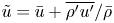$\tilde {u}=\bar {u}+\overline {\rho ^{\prime }u^{\prime }}/\bar {\rho }$, we obtain

(2.10)\begin{align} -\frac{\partial \tilde{Y}/\partial t}{\partial \tilde{Y}/\partial r}=\bar{u}+\frac{1}{\bar{\rho}}\left(\overline{\rho^{\prime}u^{\prime}}+ \frac{\boldsymbol{\nabla}\boldsymbol{\cdot}\overline{\rho Y^{\prime\prime}\boldsymbol{u}^{\prime\prime}}}{\partial \tilde{Y}/\partial r}\right)-\frac{1}{\bar{\rho}\,\partial\tilde{Y}/\partial r}\,\boldsymbol{\nabla}\boldsymbol{\cdot}\left(\bar{\rho}D\,\frac{\partial \tilde{Y}}{\partial r}+\overline{\rho D\,\frac{\partial Y^{\prime\prime}}{\partial r}}\right)\boldsymbol{e}_{\boldsymbol{r}}. \end{align}

By combining (2.5) and (2.10), we obtain

(2.11)\begin{equation} \dot{R}|_{Y_{0}}=(\bar{u}+u_{{Pen}}+u_{{Diff}})|_{Y_{0}}, \end{equation}

where

(2.12a)$$\begin{gather} u_{{Pen}}=\frac{1}{\bar{\rho}}\left(\overline{\rho^{\prime}u^{\prime}}+ \frac{\partial\overline{\rho Y^{\prime\prime}u^{\prime\prime}}/\partial r}{\partial \tilde{Y}/\partial r} \right)+u_{{Pen,G}}, \end{gather}$$

(2.12b)$$\begin{gather}u_{{Diff}}={-}\frac{1}{\bar{\rho}\,\partial\tilde{Y}/\partial r}\,\frac{\partial}{\partial r}\left(\bar{\rho}D\,\frac{\partial \tilde{Y}}{\partial r}+\overline{\rho D\,\frac{\partial Y^{\prime\prime}}{\partial r}}\right)+u_{{Diff,G}}. \end{gather}$$

Here, $\bar {u}|_{Y_{0}}$ is the Reynolds-averaged velocity at radius $r$ with $\tilde {Y}_{l}(r)=Y_0$; $u_{Pen}$ describes the contribution of the fluctuation field, $u_{{Diff}}$ represents the contribution of the molecular diffusion, and $u_{{Pen,G}}$ and $u_{{Diff,G}}$ are the terms caused by the spatial divergence in non-Cartesian coordinates, where

(2.13a)$$\begin{gather} u_{{Pen,G}}=\frac{\alpha}{\bar{\rho}}\,\frac{\overline{\rho Y^{\prime\prime}u^{\prime\prime}}/r}{\partial \tilde{Y}/\partial r}, \end{gather}$$

(2.13b)$$\begin{gather}u_{{Diff,G}}={-}\frac{\alpha}{\bar{\rho}\,\partial \tilde{Y}/\partial r}\,\frac{1}{r}\left(\bar{\rho}D\,\frac{\partial \tilde{Y}}{\partial r}+\overline{\rho D\,\frac{\partial Y^{\prime\prime}}{\partial r}}\right), \end{gather}$$

where $\alpha$ is the geometry coefficient, with $\alpha =0,1,2$ for the Cartesian, cylindrical and spherical coordinates, respectively.

At two ends of the mixing zone, the term related to the fluctuation terms, i.e. $u_{{Pen,G}}$, is negligible compared with the terms related to the spatial gradient of the fluctuation terms (the validation can be found in figures 8 and 9). Combining (2.1) and (2.11), the growth rate of the mixing width is decomposed into

(2.14)\begin{equation} \dot{W}={\rm sgn}(A)\left[(\bar{u}|_{B}-\bar{u}|_{S})+(u_{{Pen}}|_{B}-u_{{Pen}}|_{S})+(u_{{Diff}}|_{B}-u_{{Diff}}|_{S})\right], \end{equation}

which is referred to as the decomposition formula. The formula indicates that the growth of the mixing width contains three parts.

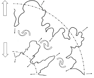
1. (i) The stretching or compression (S(C)) effect defined as the mean-velocity difference between two edges of the mixing zone, which is presented as the large arrows in figure 1. When this term is not zero, the mixing zone is stretched or compressed.

2. (ii) The penetration effect defined by the fluctuating field. This effect is illustrated in figure 1 with small arrows. During the growth of the mixing zone, $\overline {\rho Y^{\prime \prime }u^{\prime \prime }}$ and $\overline {\rho ^{\prime }u^{\prime }}$ are dominated by two important processes: the light fluid penetrates the heavy fluid, and the heavy fluid penetrates the light fluid (Li et al. Reference Li, Tian, He and Zhang2021).

3. (iii) The diffusion effect caused by molecular diffusion, which tends to decrease the density gradient at the material interface.

Figure 1. Schematic diagram of the growth of the mixing width in convergent geometry. The large arrows represent the mean velocity calculated at the bubble front and spike front. The small arrows represent the fluctuating velocity of the bubble and spike.

According to the work of Li et al. (Reference Li, Tian, He and Zhang2021), the contribution of the diffusion effect is negligible in the flows at a high Reynolds number. Therefore, in the present work, we consider only the penetration effect and the S(C) effect.

The decomposition formula provides a method to analyse quantitatively the mechanisms controlling the evolution of the mixing width in interfacial fluid mixing. In the planar geometry, the perturbation growth caused by RT/RM instability is attributed to the penetration effect in most cases, while the S(C) effect, which is a growth mechanism independent of RM/RT growth, is significant only when the mixing zone is influenced by wave systems, such as shock, rarefaction and compression waves (Li et al. Reference Li, Tian, He and Zhang2021). However, in the convergent geometry, the S(C) effect is evident even when there is no wave in the mixing zone (Ge et al. Reference Ge, Zhang, Li and Tian2020). Therefore, the S(C) effect is an important difference between the interfacial mixing in planar geometry and that in convergent geometry.

2.2. Quantitative analysis of the S(C) effect

In this subsection, we consider the S(C) effect in planar, cylindrical and spherical geometries. For the fluids inside and outside the interface, the compression rates are assumed to be uniform around the interface, i.e.

(2.15a,b)\begin{equation} \gamma_{\rho,in}={-}\dot{\rho}_{in}/\rho_{in},\quad \gamma_{\rho,out}={-}\dot{\rho}_{out}/\rho_{out}. \end{equation}

The works of Bell (Reference Bell1951) and Epstein (Reference Epstein2004) are inherited in the present work, where the fluid motion is assumed to be irrotational. Therefore, there exist velocity potentials $\varPhi _{in/out}$ that satisfy a Poisson-type equation, $\Delta \varPhi _{in/out}=-\gamma _{\rho,in/out}$. The initial perturbation is formulated as a single mode with a small amplitude. These results give the velocity potentials inside and outside the interface expressed as

(2.16a)\begin{equation} \varPhi_{in/out}(r,y,t)=\varPsi_{in/out}(r,t)+\psi_{in/out}(r,y,t) \end{equation}

in Cartesian coordinates $(r,y)$,

(2.16b)\begin{equation} \varPhi_{in/out}(r,\theta,t)=\varPsi_{in/out}(r,t)+\psi_{in/out}(r,\theta,t) \end{equation}

in cylindrical coordinates $(r,\theta )$, and

(2.16c)\begin{equation} \varPhi_{in/out}(r,\theta,\varphi,t)=\varPsi_{in/out}(r,t)+\psi_{in/out}(r,\theta,\varphi,t) \end{equation}

in spherical coordinates $(r,\theta,\varphi )$. For the planar and cylindrical geometries, we disregard the $z$-dependent direction. The potential functions $\varPsi _{in/out}(r)$ describe the background flow inside and outside the interface in all geometries, which are represented respectively as

(2.17a)\begin{equation} \varPsi_{in/out}(r,t)={-}(r-R)\dot{R}-(r-R)^{2}\,\frac{\gamma_{\rho,in/out}}{2} \end{equation}

in the planar geometry,

(2.17b)\begin{equation} \varPsi_{in/out}(r,t)={-}\left(R\dot{R}-\frac{R^{2}}{2}\,\gamma_{\rho,in/out}\right)\ln r-\frac{\gamma_{\rho,in/out}}{4}\,r^{2} \end{equation}

in the cylindrical geometry, and

(2.17c)\begin{equation} \varPsi_{in/out}(r,t)=\left(R^{2}\dot{R}-\frac{R^{2}}{3}\,\gamma_{\rho,in/out}\right)\frac{1}{r}-\frac{\gamma_{\rho,in/out}}{6}\,r^{2} \end{equation}

in the spherical geometry. For consistency, we use $R$ to indicate the position of the interface throughout. Here, $\psi _{in/out}$ represents the potential of the perturbed flow, which satisfies the Laplace function $\Delta \psi _{in/out}=0$ and thus is formulated as

(2.18a)\begin{equation} \psi_{in/out}(r,y,t)=A_{in/out}(\gamma_{\rho,in/out},t)\exp({\pm2{\rm \pi} mr/L})\cos(2{\rm \pi} my /L) \end{equation}

in the planar geometry (where $m$ is the wavenumber of the perturbation, and $L$ is the length scale in the spanwise direction $y$),

(2.18b)\begin{equation} \psi_{in/out}(r,\theta,t)=A_{in/out}(\gamma_{\rho,in/out},t)\,r^{{\pm} m}\cos(m\theta) \end{equation}

in the cylindrical geometry, and

(2.18c)\begin{equation} \psi_{in/out}(r,\theta,\varphi,t)=A_{in/out}(\gamma_{\rho,in/out},t)\,r^{[m,-(m+1)]}\,Y_{m}^{n}(\theta,\varphi) \end{equation}

in the spherical geometry, where $m-n$ and $n$ are the latitude and longitude wavenumbers, respectively. Also, $A_{in/out}(t)$ is the function determined by the boundary condition and is a function of only time. The perturbed interface equations are

(2.19a)\begin{equation} r=R(t)+a(t)\cos(2{\rm \pi} my/L) \end{equation}

in the planar geometry,

(2.19b)\begin{equation} r=R(t)+a(t)\cos\left(m\theta\right) \end{equation}

in the cylindrical geometry, and

(2.19c)\begin{equation} r=R(t)+a(t)\,Y_{m}^{n}(\theta,\varphi) \end{equation}

in the spherical geometry, where $a(t)$ is the amplitude of the perturbation. Therefore, the bubble front $R_{B}$ and spike front $R_{S}$ of the mixing zone are described as $R-a$ and $R+a$, respectively. The Reynolds-averaged velocities at the bubble front and spike front in different geometries are calculated as

(2.20a)\begin{equation} \bar{u}_{B/S}=\left.-\int_{0}^{L}\frac{\partial\varPhi_{in/out}}{\partial r}(R_{B/S},y)\,\mathrm{d} y\right/\int_{0}^{L}\mathrm{d} y \end{equation}

in the planar geometry,

(2.20b)\begin{equation} \bar{u}_{B/S}=\left.-\unicode{x222E}_{\theta}\frac{\partial\varPhi_{in/out}}{\partial r}(R_{B/S},\theta)\,\mathrm{d}\theta\right/\unicode{x222E}_{\theta}\,\mathrm{d}\theta \end{equation}

in the cylindrical geometry, and

(2.20c)\begin{equation} \bar{u}_{B/S}={-}\left.\unicode{x222F}_{\theta,\varphi}\frac{\partial\varPhi_{in/out}}{\partial r}(R_{B/S},\theta,\varphi)\,\mathrm{d}\theta\,\mathrm{d}\varphi\right/ \unicode{x222F}_{\theta,\varphi}\,\mathrm{d}\theta\,\mathrm{d}\varphi \end{equation}

in the spherical geometry. As a result, we have

(2.21a)$$\begin{gather} \bar{u}_{S}=\dot{R}+a\gamma_{\rho,out}, \end{gather}$$

(2.21b)$$\begin{gather}\bar{u}_{B}=\dot{R}-a\gamma_{\rho,in} \end{gather}$$

in the planar geometry,

(2.21c)$$\begin{gather} \bar{u}_{S}=\left(R\dot{R}-\frac{R^{2}}{2}\,\gamma_{\rho,out}\right)\frac{1}{R+a}+\frac{\gamma_{\rho,out}}{2}\left(R+a\right), \end{gather}$$

(2.21d)$$\begin{gather}\bar{u}_{B}=\left(R\dot{R}-\frac{R^{2}}{2}\,\gamma_{\rho,in}\right)\frac{1}{R-a}+\frac{\gamma_{\rho,in}}{2}\left(R-a\right) \end{gather}$$

in the cylindrical geometry, and

(2.21e)$$\begin{gather} \bar{u}_{S}=\left(R\dot{R}-\frac{R^{2}}{3}\,\gamma_{\rho,out}\right)\frac{1}{\left(R+a\right)^{2}}+\frac{\gamma_{\rho,out}}{3}\left(R+a\right), \end{gather}$$

(2.21f)$$\begin{gather}\bar{u}_{B}=\left(R\dot{R}-\frac{R^{2}}{3}\,\gamma_{\rho,in}\right)\frac{1}{\left(R-a\right)^{2}}+\frac{\gamma_{\rho,in}}{3}\left(R-a\right) \end{gather}$$

in the spherical geometry. Substituting (2.21) into (2.14) and considering that $a\ll R$, one obtains that the S(C) effect is formulated as

(2.22)\begin{equation} \dot{W}_{S(C)}=(\alpha\gamma_{R}+\gamma_{\rho})W, \end{equation}

where $\gamma _{\rho }=(\gamma _{\rho,out}+\gamma _{\rho,in})/2$, the averaged compression rate, and $W=2a$ denotes the mixing width. The geometrical coefficient is $\alpha =0,1,2$ for the planar, cylindrical and spherical geometries, and $\dot {W}_{S(C)}>0$ means that the mixing zone is stretched, while $\dot {W}_{S(C)}<0$ means that the mixing width is compressed.

The interface convergence gives $\gamma _{R}>0$, and fluid compression gives $\gamma _{\rho }<0$. Therefore, the geometrical convergence leads to the stretching of the mixing zone, while fluid compression leads to the compression of the mixing zone. The coupling of geometrical convergence and fluid compression is realized by the linear superposition. Furthermore, in cylindrical geometry $\alpha =1$, while in spherical geometry $\alpha =2$. Therefore, the contribution from the geometrical convergence is more significant in the spherical geometry.

2.3. Physical origin of the S(C) effect

According to (2.22), the S(C) effect is determined by three physical quantities: $\gamma _{R}$, $\gamma _{\rho }$ and $W$. As will be shown, the underlying physical origin of (2.22) is that the mass in the mixing zone is conserved except for the mass brought in by the penetration effect.

As shown in figure 2, the mass in the mixing zone is $\rho V_{t}$ at time $t$, and $(\rho +\Delta \rho )V_{t+\Delta t}$ at time $t+\Delta t$. Here, $V_{t}$ denotes the volume of the mixing zone at time $t$. In this demonstration, $\rho$ is assumed to be uniform in the mixing zone. For the cylindrical geometry, we have $V_{t}={\rm \pi} [(R+W/2)^{2}-(R-W/2)^{2}]=2{\rm \pi} WR$, where the axial length is unity. For the spherical geometry, we have $V_{t}=({4{\rm \pi} }/{3})[(R+W/2)^{3}-(R-W/2)^{3}]=4{\rm \pi} WR^{2}(1+{W}/{12R})$. By assuming that the mass in the mixing zone is conserved, we have $\rho V_{t}=(\rho +\Delta \rho )V_{t+\Delta t}$, i.e.

(2.23a)\begin{equation} 2{\rm \pi}\rho WR=2{\rm \pi}\left(\rho+\Delta\rho\right)\left(W+\Delta W\right)\left(R+\Delta R\right) \end{equation}

in the cylindrical geometry, and

(2.23b)\begin{align} 4{\rm \pi}\rho WR^{2}\left(1+\frac{W}{12R}\right)= 4{\rm \pi}\left(\rho+\Delta\rho\right)\left(W+\Delta W\right)\left(R+\Delta R\right)^{2}\left(1+\frac{W+\Delta W}{12(R+\Delta R)}\right) \end{align}

in the spherical geometry. In most cases, the radial length of the mixing zone is much smaller than the radius. Therefore, $W/12R\ll 1$. By disregarding small quantities of any order higher than the first, we obtain

(2.24)\begin{equation} \Delta W={-}\left(\frac{\Delta\rho}{\rho}+\alpha\,\frac{\Delta R}{R}\right)W, \end{equation}

where $\alpha =1,2$ for the cylindrical geometry and spherical geometry, respectively. Dividing (2.24) by $\Delta t$ and applying $\Delta t\to 0$, we have $\dot {W}_{S(C)}=(\alpha \gamma _{R}+\gamma _{\rho })W$, which is the same as (2.22). Therefore, we verify that the S(C) effect originates from the idea that the mass in the mixing zone is conserved if we do not consider the mass brought in by the penetration effect. When the mixing zone undergoes fluid compression or interface convergence, the density or the spanwise length of the mixing zone changes, and the mixing width changes as well.

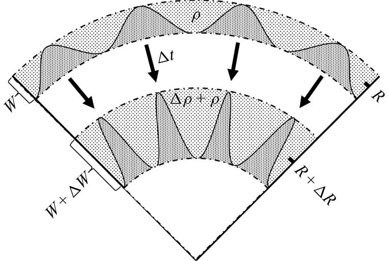
Figure 2. Schematic diagram of the S(C) effect. At time $t$, the mixing zone is positioned in the radius $R$ with width $W$, where $R$ is the centre radius of the mixing zone. The density $\rho$ in the mixing zone is assumed to be uniform. After $t+\Delta t$, the mixing zone converges to radius $R+\Delta R$ with width $W+\Delta W$ and density $\rho +\Delta \rho$.

2.4. The S(C) effect and the BP effect

According to (2.22), the S(C) effect is caused by the geometrical convergence and fluid compression. For the geometrical convergence, it happens in only cylindrical and spherical geometries. For the fluid compression, it happens in a convergent system where the fluids are compressed, or when the mixing zone is influenced by waves, such as shock waves, rarefaction waves and compression waves. Therefore, we know that in planar geometry, $\dot {W}_{S(C)} = 0$ when there is no wave system acting on the mixing zone (Li et al. Reference Li, Tian, He and Zhang2021), while $\dot {W}_{S(C)} \ne 0$ in convergent geometries (Ge et al. Reference Ge, Zhang, Li and Tian2020). Therefore, we conclude that the S(C) effect is an important part of the BP effect.

However, the S(C) effect is not equivalent to the BP effect. The BP effect is, in fact, a collective factor for the modification caused by the geometry, which contains multiple mechanisms. For example, as the interface converges, the wavelength of the perturbations changes, and how this factor modifies the instability remains an open question.

In this section, we give the definition of the S(C) effect in (2.14). The quantitative relation between the S(C) effect and the geometrical convergence and fluid compression is given in (2.22), which implies that the S(C) effect originates from the conservation of the mixing mass. Furthermore, we prove that the S(C) effect is one of the mechanisms of the BP effect. In the next section, a series of numerical simulations is provided to support our theoretical analysis.

3.1. Governing equations and computational approach

The flow field is governed by the compressible multi-component Navier–Stokes equations. The mass, momentum, energy and mass fraction equations are

(3.1a)$$\begin{gather} \frac{\partial\rho}{\partial t} + \boldsymbol{\nabla}\boldsymbol{\cdot}(\rho\boldsymbol{u})=0, \end{gather}$$

(3.1b)$$\begin{gather}\frac{\partial\rho\boldsymbol{u}}{\partial t}+\boldsymbol{\nabla}\boldsymbol{\cdot}(\rho\boldsymbol{u}\boldsymbol{u})={-}\boldsymbol{\nabla} \boldsymbol{\cdot}(p\boldsymbol{\delta}-\boldsymbol{\tau}), \end{gather}$$

(3.1c)$$\begin{gather}\frac{\partial\rho E}{\partial t}+\boldsymbol{\nabla}\boldsymbol{\cdot}(\rho E\boldsymbol{u})={-}\boldsymbol{\nabla}\boldsymbol{\cdot}\left(p\boldsymbol{u}-\boldsymbol{\tau}\boldsymbol{\cdot}\boldsymbol{u}-\kappa\,\boldsymbol{\nabla}T-T\sum_{i} C_{p,i}(\rho D\,\boldsymbol{\nabla}Y_{i})\right), \end{gather}$$

(3.1d)$$\begin{gather}\frac{\partial\rho Y_{i}}{\partial t}+\boldsymbol{\nabla}\boldsymbol{\cdot}(\rho Y_{i}\boldsymbol{u})=\boldsymbol{\nabla}\boldsymbol{\cdot}(\rho D\,\boldsymbol{\nabla}Y_{i}), \end{gather}$$

where $\rho$, $\boldsymbol {u}$, $p$, and $T$ are the density, velocity vector, pressure and temperature, respectively. The energy of the fluid is 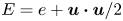$E=e+\boldsymbol {u}\boldsymbol {\cdot }\boldsymbol {u}/2$, where $e$ is the internal energy, and $\boldsymbol {u}\boldsymbol {\cdot }\boldsymbol {u}/2$ is the kinetic energy. Here, $\boldsymbol {\delta }$ is the Kronecker function, $Y_i$ is the mass fraction of the $i$th species, where $i=1,2$ and $Y_{1}+Y_{2} =1$, $\kappa$ and $D$ are the mixture thermal conductivity and the mixture diffusion coefficient, respectively, and $C_{p,i}$ is the constant-pressure-specific heat capacity of the $i$th species. To close the equations, the fluids are assumed to be Newtonian to calculate the shear stress, and the equations of state for the ideal gas are applied, i.e.

(3.2a)$$\begin{gather} \boldsymbol{\tau}=\mu\left(\boldsymbol{\nabla}\boldsymbol{u}+(\boldsymbol{\nabla}\boldsymbol{u})^{\rm{T}}- \tfrac{2}{3}\boldsymbol{\delta}(\boldsymbol{\nabla}\boldsymbol{\cdot}\boldsymbol{u})\right), \end{gather}$$

(3.2b)$$\begin{gather}\frac{p}{\rho}=\frac{e}{\gamma-1}, \end{gather}$$

where $\gamma =C_{p}/C_{V}$ is the heat capacity ratio, and $C_{V}$ is the constant-volume-specific heat capacity.

The viscosity, thermal conductivity, and diffusivity of the $i$th species, which describe the physical properties of the component, are obtained as (Sutherland Reference Sutherland1893),

(3.3a)$$\begin{gather} \mu_{i}=\mu_{0,i}\left(\frac{T}{T_{0}}\right)^{3/2}\frac{T_{0}+T_{s}}{T+T_{s}}, \end{gather}$$

(3.3b)$$\begin{gather}\kappa_{i}=C_{p,i}\,\frac{\mu_{i}}{{Pr}_{i}}, \end{gather}$$

(3.3c)$$\begin{gather}D_{i}=\frac{\mu_{i}}{\rho_{i}\,{Sc}_{i}}, \end{gather}$$

where $\mu _{0,i}$ is the viscosity at a reference temperature $T_{0}=273.15\ {\rm K}$, $T_{s}=124\ {\rm K}$ is an effective temperature (Li et al. Reference Li, He, Zhang and Tian2019), and ${Pr}_{i}$ and ${Sc}_{i}$ are the Prandtl number and Schmidt number for the $i$th species, respectively.

The thermodynamic quantities $f$ of the mixture in a computational cell are calculated following Reckinger, Livescu & Vasilyev (Reference Reckinger, Livescu and Vasilyev2016):

(3.4) \begin{equation} f=\left\{\begin{array}{@{}ll} \displaystyle\sum_{i}f_{i}, & {\rm for}\ f=\rho, p,\\[3pt] f_{1}=\dots=f_{i}, & {\rm for}\ f=T,V,\\[3pt] \displaystyle\sum_{i}Y_{i}f_{i}, & {\rm for}\ f=\mu,\kappa,D,C_{V},C_{p}. \end{array}\right. \end{equation}

The governing equations are solved numerically by the finite difference method with the program APEX (Adaptive-mesh-refinement Program of Eulerian solvers with X-physics). To show the reliability in simulating RM instability with APEX, we simulate the case taken from the work of Thornber et al. (Reference Thornber2017). Appendix A shows the numerical results and their comparison with other algorithms. The fifth-order weighted essentially non-oscillation (WENO) scheme is adopted for spatial reconstruction. The Harten–Lax–van Leer contact (HLLC) approximate Riemann solver is applied to calculate the convection flux. The time advancement is achieved through a third-order Runge–Kutta scheme.

3.2. Initial problem set-up

3.2.1. Computational domain

In this subsubsection, we first simulate the RM instability in a cylindrical geometry. To compare the influence of geometry, RM instability in a planar geometry is also simulated, in which the perturbed interface is the same as that unfolded from the cylindrical interface. Both two-dimensional (2-D) and three-dimensional (3-D) cases are simulated. All cases are simulated under Cartesian grids ($(x,y)$ for 2-D cases, and $(x,y,z)$ for 3-D cases). The 2-D views of both configurations are depicted in figure 3. By comparing the subsequent growth of the perturbations on the two interfaces after shock time $t_{0}$, we can evaluate the influence caused by the geometry.

Figure 3. Planar slice at $z = 0$ for (a) cylindrical geometry and (b) planar geometry.

The initial setting of the cylindrical case is shown in figure 3(a). At the initial time $t^{-}$, the material interface is located at the position $r=R_{0}$. The convergent shock wave radius is $R_{s}(t^{-})=R_{s0}=1.1R_{0}$, and the domain size $\mathcal {V}_{{cylinder}}$ is

(3.5a)$$\begin{gather} \mathcal{V}_{{cylinder}, 2\text{-}D}=\{(x,y)\,\vert\,\vert x\vert \leqslant R_{ext},\,\vert y\vert \leqslant R_{ext}\}, \end{gather}$$

(3.5b)$$\begin{gather}\mathcal{V}_{{cylinder}, 3\text{-}D}=\{(x,y,z)\,\vert\, \vert x\vert \leqslant R_{ext},\,\vert y\vert \leqslant R_{ext},\,\vert z\vert \leqslant {\rm \pi}R_{0}\}, \end{gather}$$

with $R_{ext}=4{\rm \pi} R_{0}$ to avoid possible influence caused by the boundaries. The symmetric boundaries are set in the axial direction $z$, while outflow conditions are applied in the $x$ and $y$ directions. The convergence analysis of the size of the computational domain is presented in Appendix B.

The initial setting of the planar case is shown in figure 3(b). The planar interface is obtained by unfolding the cylindrical interface, including the perturbations. The planar case considered is a shock tube with a constant cross-section. At the initial time $t^{-}$, the material interface is located at the position $x=R_{0}$. The initial shock wave locates at $R_{s}(t^{-})=R_{s0}$, and the domain size $\mathcal {V}_{{plane}}$ is

(3.6a)$$\begin{gather} \mathcal{V}_{{plane}, 2\text{-}D}=\{(x,y)\,\vert\,R_{ext}^{-}\leqslant x \leqslant R_{ext}^{+},\,\vert y\vert \leqslant {\rm \pi}R_{0}\}, \end{gather}$$

(3.6b)$$\begin{gather}\mathcal{V}_{{plane}, 3\text{-}D}=\{(x,y,z)\,\vert\, R_{ext}^{-}\leqslant x \leqslant R_{ext}^{+},\,\vert y\vert \leqslant {\rm \pi}R_{0},\,\vert z\vert \leqslant {\rm \pi}R_{0}\}, \end{gather}$$

where $R_{ext}^{+}-R_{ext}^{-}\;=\;2R_{ext}$. We adjust $R_{ext}^{-}$ to make sure that the re-shock time when the reflected shock wave impacts the interface is identical in the two geometries. An outflow boundary condition is applied at $x = R_{ext}^{+}$, while a symmetric boundary condition is used at $x = R_{ext}^{-}$. Periodic boundaries are applied in the $y$ direction. The boundaries in the $z$ direction are symmetric.

The streamwise direction refers to the direction in which the shock wave propagates, i.e. the radial direction in the cylindrical cases, and the $x$ direction in the planar cases. The spanwise direction denotes the direction perpendicular to the streamwise direction.

For the 2-D cylindrical cases, the base grid resolution is $4096^{2}$, and four additional levels of refinement with a factor of two are applied. The finest resolution is therefore $65\,536^{2}$, i.e. $\Delta x_{min}\approx 3.8\times 10^{-4}R_{0}$. The same $\Delta x_{min}$ and refinement level are applied for the planar cases, i.e. the base grid resolution is $4096\times 1024$ ($x\ {\rm direction}\times y\ {\rm direction}$) for the 2-D planar cases. For the 3-D cylindrical cases, the base grid resolution is $512\times 512\times 128$ ($x\ {\rm direction}\times y\ {\rm direction} \times z\ {\rm direction}$), and five additional levels of refinement with a factor of two are applied. The finest resolution is therefore $16\,384\times 16\,384\times 4096$, i.e. $\Delta x_{min}\approx 1.5\times 10^{-3}R_{0}$ in both domains. The same $\Delta x_{min}$ and refinement level are applied for the planar cases, i.e. the base grid resolution is $512\times 128\times 128$ for the 3-D planar cases. The grid convergence analysis is presented in Appendix B.

3.2.2. Initial fluid state

The two fluids considered here are air (fluid 1, outside the interface) and ${\rm SF}_{6}$-acetone mixtures (fluid 2, inside the interface). As with Tritschler et al. (Reference Tritschler, Olson, Lele, Hickel, Hu and Adams2014), the unshocked state parameters and other properties of the two fluids are shown in table 1.

Table 1. The preshock state parameters and other properties of fluid 1 (air) and fluid 2 (${\rm SF}_{6}$-acetone).

For the cylindrical configuration, the initialization of the postshock fluid refers to the work of Chisnell (Reference Chisnell1998). In that work, by solving the mass, momentum and entropy equations for postshock symmetric flow, using an adiabatic ideal gas assumption, the self-similar solutions of $\rho$, $p$, $\boldsymbol {u}$ are given in terms of $\xi =r/R_{s}$, where $R_{s}$ is the radius of the shock wave. For both geometries, the preshock and postshock states satisfy the Rankine–Hugoniot conditions.

For the cylindrical geometry, the initial Mach number of the shock wave is set to ensure a large convergence ratio ($C_{r}\sim 10$) before the interface is re-shocked. Meanwhile, the non-dimensional duration (defined in the next section) when the interface converges with a quasi-steady velocity should be long enough so that the cylindrical and planar cases are comparable. Hence the initial Mach number of the cylindrical shock wave is set to be 2.

For the planar geometry, the Mach number is adjusted so that the velocity jump of the interface $\Delta V$ impacted by the incident shock is the same as that in the cylindrical geometry. In the cylindrical geometry, when the shock wave arrives at the interface at $r = R_{0}$, the Mach number is greater than the Mach number at the initial time $t^{-}$, i.e. ${Ma}(t_{0})>{Ma}(t^{-})$. By referring to the work of Si et al. (Reference Si, Long, Zhai and Luo2015), we can predict the Mach number of the convergent shock wave at the shock time $t_{0}$. Based on this theoretical value, the Mach number is adjusted slightly and it is finally set to be ${Ma}_{{plane}}=2.14$ in the numerical simulations.

3.2.3. Initial perturbations

Two types of initial perturbations are applied: (i) single-mode perturbation in 2-D cases, and (ii) multi-mode perturbation in 3-D cases.

The single-mode perturbations at both interfaces are presented as

(3.7)\begin{equation} \eta_{{cylinder}}(\theta)=a_{m}\cos(k_{m}\theta R_{0}) \end{equation}

and

(3.8)\begin{equation} \eta_{{plane}}(y)=a_{m}\cos(k_{m}y), \end{equation}

where $a_{m}$ is the amplitude of perturbation, and $k_{m}=mk_{0}$, with $m$ the wavenumber and $k_{0}=2{\rm \pi} /(2{\rm \pi} R_{0})=1/R_{0}$. Two wavenumbers are applied: $m=8$ and $m=16$, which are named SP8 and SP16, respectively. The initial amplitude is $a_{m}=0.01\lambda _{m}$, where $\lambda _{m}=2{\rm \pi} R_{0}/m$.

The multi-mode perturbation is a superposition of a series of modes with a prescribed power spectrum (Dimonte et al. Reference Dimonte2004). The power spectrum is given as

(3.9)\begin{equation} P(k)=\begin{cases} Fk^{l}, & k_{min}< k< k_{max}, \\ 0, & \text{otherwise}, \end{cases} \end{equation}

where $k=\sqrt {k_{m}^{2}+k_{n}^{2}}$ denotes the wavenumber of the mode $(m,n)$, and $F$ is the coefficient. In physical space, the perturbations are of the form

(3.10) \begin{align} \eta_{{cylinder}}(\theta,z)=\sum_{m,n}&\bigl(a_{mn}\cos(k_{m}\theta R_{0})\cos (k_{n}z)+b_{mn}\sin(k_{m}\theta R_{0})\cos(k_{n}z)\nonumber\\ &\quad +c_{mn}\cos(k_{m}\theta R_{0})\sin(k_{n}z)+d_{mn}\sin(k_{m}\theta R_{0})\sin(k_{n}z)\bigr) \end{align}

and

(3.11) \begin{align} \eta_{{plane}}(y,z)=\sum_{m,n}&\bigl(a_{mn}\cos(k_{m}y)\cos(k_{n}z)+b_{mn}\sin(k_{m}y)\cos(k_{n}z) \nonumber\\ &\quad +c_{mn}\cos(k_{m}y)\sin(k_{n}z)+d_{mn}\sin(k_{m}y)\sin(k_{n}z)\bigr), \end{align}

where the amplitude coefficients $a_{mn}$, $b_{mn}$, $c_{mn}$ and $d_{mn}$ are determined by the variance $\sigma ^{2}_{mn}\sim P(k_{m},k_{n})\,\Delta k_{m}\Delta k_{n}$, which corresponds to the energy involved in wave space, and $k_{m}=mk_{0}$ and $k_{n}=nk_{0}$, where $k_{0}=2{\rm \pi} /(2{\rm \pi} R_{0})=1/R_{0}$. The relevant detailed demonstration of the transformation from the wave space (3.9) to the physical space (3.10) and (3.11) has been given by Thornber et al. (Reference Thornber, Drikakis, Youngs and Williams2010). In the present work, a narrowband perturbation with wavenumbers ranging from 16 to 48 is used, and the energy spectrum follows $P(k)=Fk^{0}$. The total standard deviation is $\sigma =\sqrt {\int P(k)\,{\rm d}k}\approx 0.0067R_{0}$. These cases are named MP16–48.

4.1. One-dimensional unperturbed flow

In this section, we inspect the one-dimensional unperturbed cases, with an emphasis on the periods before the re-shock moment $t_{rs}$. Figure 4 shows the interface motion $R(t)$ in both geometries. The interface has a non-zero width because of the numerical diffusion, therefore the position of the interface $R(t)$ is defined as the radius where $Y_{1}(R(t),t)=0.5$. The curves obtained from the planar case are shifted along the time axis so that the shock time $t_s$ is aligned. The interface is shocked at time $t_{s}=0.4\ {\rm ms}$, then the planar interface moves with a constant velocity $\Delta V =340\ {\rm m}\ {\rm s}^{{-1}}$ until the interface is re-shocked at $t_{rs}=8.5\ {\rm ms}$. For the cylindrical case, before $t_{1}=5\ {\rm ms}$, the convergence velocity is slightly increased, and after that, the interface begins to decelerate. At re-shock time $t_{rs}$, the final convergence ratio of the interface is $C_{r}(t_{rs})\sim 10$.

Figure 4. The displacement (a) and velocity (b) of the interface.

The temporal evolution of the averaged fluid compression rate $\gamma _{\rho }$ is plotted in figure 5, where the density value is sampled from two sides of the interface. At time $t_{s}$, the interface is shocked by the shock wave, which results in a strong compression of the fluids. For time $t\in [t_{s},t_{0}]$, where $t_{0}=1$ ms, the shock wave continues to affect the fluids near the interface, which results in the negative pulse of the fluid compression. After $t_{0}$, the planar RM flow is quasi-incompressible before the re-shock, which supports the discussion in § 2.4. Fluid compression is one of the basic features of convergent RM instability. Therefore, for cylindrical cases, after $t_{0}$, a non-zero fluid compression rate can still be observed, and its absolute value continues to rise with the convergence of the interface.

Figure 5. The temporal evolution of the fluid compression rate.

According to the evolution of the fluid parameters mentioned above, the flow evolution is divided into five stages, as shown in table 2. Due to the nature of the convergent shock wave, the acceleration of the convergent interface is not zero. Therefore, the growth of perturbations in the convergent geometries is coupled with RT stability/instability. RT instability, as introduced in § 1, is the phenomenon where the perturbation grows in an acceleration environment (the lighter fluid accelerates the heavier fluid), while the RT stability is the situation when the heavier fluid accelerates the lighter fluid and the perturbations oscillates or attenuates.

Table 2. Definition of five stages of the RM instability until the re-shock time.

The quantities presented in the following subsections are non-dimensionalized. For the single-mode cases, the characteristic length is the initial wavelength of the perturbation, $L^{*}=\lambda$. The characteristic velocity is 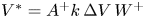$V^{*}=A^{+}k\,\Delta V\,W^{+}$, where $W^{+}=(1-\Delta V/V_{s})\,W(t^{-})$, and $V_{s}$ is the velocity of the shock wave. For the multi-mode cases, the characteristic velocity is defined as the growth rate of the perturbations at time $t_{0}$ when the shock wave just passes away from the interface. The characteristic length is $L^{*}=\bar {\lambda }$, where $\bar {\lambda }=2{\rm \pi} /\bar {k}$ is the equivalent wavelength of the perturbations at time $t^{-}$, and $\bar {k}$ is calculated by the energy-weighted average of $k$, which is formulated as

(4.1)\begin{equation} \bar{k}=\frac{\displaystyle\int_{k_{min}}^{k_{max}}k\,P(k)\,\mathrm{d}k}{\displaystyle\int_{k_{min}}^{k_{max}}P(k) \,\mathrm{d}k}. \end{equation}

In this paper, $P(k)=Ck^{0}$, hence $\bar {k}=0.5(k_{min}+k_{max})$. The characteristic quantities for all of the cases are listed in table 3.

Table 3. Characteristic quantities for each case.

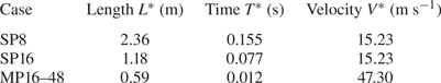
4.2. Single-mode cases

Figures 6 and 7 show the growth of the perturbations for the cases SP8 and SP16, respectively. After $\tau =\tau _{0}$ when the shock wave passes away from the interface, the initial growth rates are identical in both geometries, as designed in § 3. Because the initial amplitude of the perturbations is set as $a_{m}=0.01\lambda _{m}$, the growth of the perturbations lies in the linear stage.

Figure 6. For the case SP8, the temporal evolution of the mixing width, as well as its growth rate, in both geometries.

Figure 7. For the case SP16, the temporal evolution of the mixing width, as well as its growth rate, in both geometries.

For the planar configurations, the growth rate of the perturbations increases slowly and is smaller than the growth rate predicted by the linear theory (Richtmyer Reference Richtmyer1960) by the time $t_{rs}$, i.e. the non-dimensional growth rate is smaller than 1. This shows that the growth of the perturbations is still in the start-up process (Lombardini & Pullin Reference Lombardini and Pullin2009). For the cylindrical configurations, the temporal evolution of the perturbation growth rate is significantly different from that of the planar configurations. The growth rate in the cylindrical geometry is first accelerated and then decelerated to a negative value. This complicated growth behaviour in the cylindrical geometry originates from the coupling of multiple physical effects (for example, the RT instability/stability, geometrical convergence, and fluid compression).

The decomposition formula (2.14) is applied to decompose the growth of the perturbations, where the contribution of the diffusion is neglected. The results are given in figures 8 and 9. In all configurations, the results obtained by the decomposition formula $\dot {W}_{formula}$ and the results extracted directly from the numerical simulations $\dot {W} _{sim}$ are consistent, which proves the reliability of the decomposition formula. Furthermore, in figures 8(b) and 9(b), we have $\dot {W}_{Pen,G}=u_{Pen,G}\vert _{B}-u_{Pen,G}\vert _{S}\approx 0$, where $u_{Pen,G}$ is defined in (2.13), which is neglected in the following analysis.

Figure 8. For the case SP8, the growth rates obtained by the simulation and the decomposition formula for (a) planar geometry and (b) cylindrical geometry.

Figure 9. For the case SP16, the growth rates obtained by the simulation and the decomposition formula for (a) planar geometry and (b) cylindrical geometry.

For the planar cases, one can observe that $\dot {W}_{S(C)}$, which represents the contribution of the S(C) effect, is not zero only when the wave system acts on the mixing zone. For most of the time in the duration $[\tau _{0},\tau _{rs}]$, the growth of the mixing width is dominated by the penetration effect, as shown in figures 8(a) and 9(a), which is consistent with the previous work of Li et al. (Reference Li, Tian, He and Zhang2021). For the cylindrical geometry, at the initial time, $\dot {W}_{S(C)}(\tau _{0})=0$. However, with the evolution of the flow, the contribution of the S(C) effect continues to increase and finally exceeds the penetration effect to dominate the growth of the perturbations. From the numerical results, we know that the S(C) effect is very different in the two geometries, therefore the S(C) effect is an important part of the BP effect.

The comparisons of the penetration effect are shown in figure 10. In both geometries, the $\dot {W}_{Pen}$ values are identical at the initial time. With the coupling effect of geometrical convergence and the RT instability, the fluid penetration effect increases before the convergent velocity reaches its maximum $\tau _{1}$. After that, under the influence of the RT stability, the penetration rate decreases to a negative value at late time.

Figure 10. For (a) the case SP8 and (b) the case SP16, the different performances of the penetration effect in the two geometries.

The evolution of the S(C) effects is shown in figure 11. The values of $\gamma _{\rho }$ and $\gamma _{R}$ used in (2.22) are obtained from the one-dimensional unperturbed simulations. The numerical results and the theory agree well, which proves the reliability of the theory.

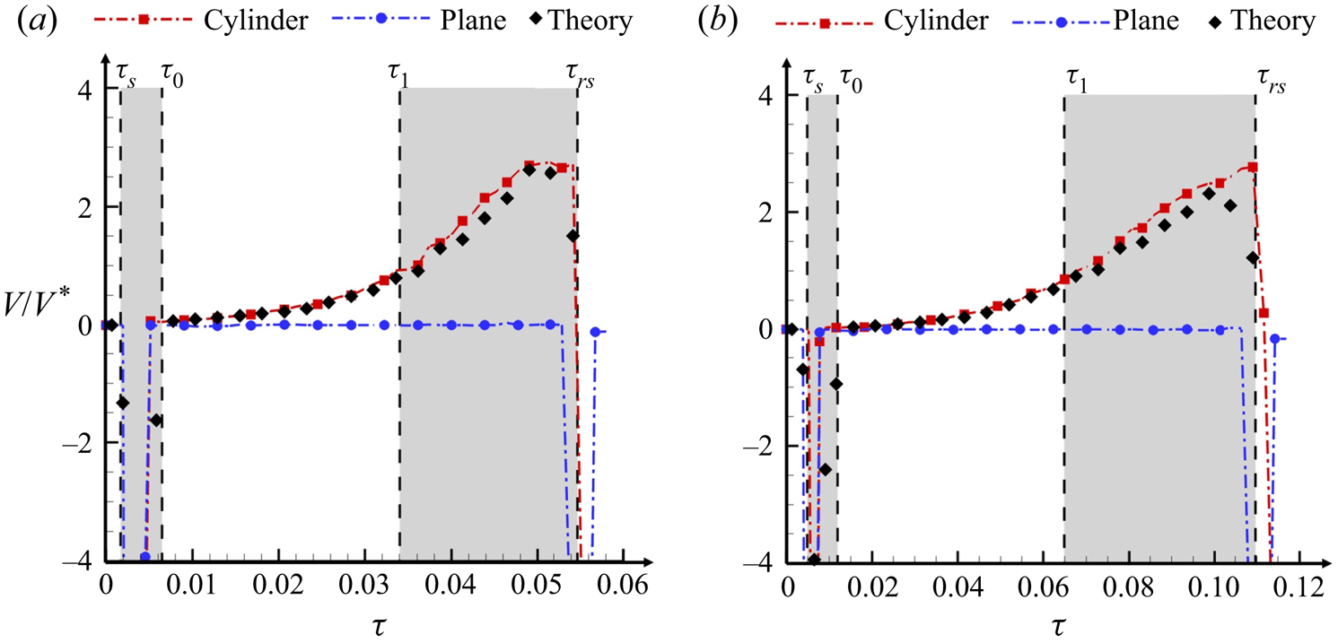
Figure 11. For (a) the case SP8 and (b) the case SP16, the evolution of the S(C) effect in the two geometries. The theoretical prediction for the S(C) effect in the cylindrical geometry is also shown.

The stretching effect ($V_{Stretching}=\gamma _{R}W$) and the compression effect ($V_{Compression}=\gamma _{\rho }W$) are given in figure 12. In the short duration $\tau \in [\tau _{s},\tau _{0}]$, the perturbations are compressed strongly by the shock wave. Therefore, the S(C) effect is dominated by the compression effect caused by the shock wave. In the duration $\tau \in [\tau _{0},\tau _{rs}]$, the stretching velocity is always greater than the compression velocity, with the ratio $|V_{Stretching}/V_{Compression}|$ ranging from 1 to 2.

Figure 12. For (a) the case SP8 and (b) the case SP16, the contributions of different components in the S(C) effect of the cylindrical cases.

4.3. Multi-mode case

To examine the universality of the results obtained from the single-mode cases, the multi-mode cases are simulated. Figure 13 gives the growth of the perturbations for the cases MP16–48. For the planar configuration, after $\tau =\tau _{0}$, there is no more energy injected into the system. Therefore, in the duration $\tau \in [\tau _{0},\tau _{1}]$, the growth rate of the perturbations first experiences a short-time increase and then attenuates. For the cylindrical configuration, it is obvious that the convergent interface enhances the growth of the perturbations. In the duration $\tau \in [\tau _{0},\tau _{1}]$, the growth rate of the perturbations does not decay, in contrast with that in the planar geometry. During the subsequent duration $\tau \in [\tau _{1},\tau _{rs}]$, the acceleration of the interface is pointed from the heavy fluid to the light fluid; hence the growth of the perturbations is influenced by the RT stability, which decelerates the growth of the perturbations.

Figure 13. For the cases MP16–48, the temporal evolution of the mixing width, as well as its velocity, in both geometries.

Figure 14 shows the growth rates obtained with the decomposition formula and those obtained from the numerical results in both geometries. In both geometries, at time $\tau _{s}$ when the incident shock wave impacts the interface, $\dot {W}_{S(C)}$ experiences a sharp decrease due to the compression by the shock wave. Meanwhile, the incidence shock wave deposits vorticity on the interface, which results in an increase in the penetration effect $\dot {W}_{Pen}$.

Figure 14. For the cases MP16–48, the growth rates obtained by the simulation and the decomposition formula for (a) planar geometry and (b) cylindrical geometry.

For the planar configuration, $\dot {W}_{S(C)}$ is always zero when $\tau \in [\tau _{0},\tau _{rs}]$, which indicates that the growth of the mixing width is dominated by the penetration effect if there is no influence of the wave system. For the cylindrical configuration, with the convergence of the interface, the stretching effect of the mixing width continues to increase. When $\tau >\tau _{1}$, the contribution of the penetration effect decreases due to the RT stability, while the stretching effect surpasses the penetration effect and begins to dominate the perturbation growth.

Figure 15(a) shows the evolution of the penetration effect in the two geometries. After the passage of the shock wave, as the initial growth rates are the same, the penetration rates in both geometries are identical. In the subsequent duration $\tau \in [\tau _{0},\tau _{1}]$, the penetration rates increase first and then decay with almost the same rate in both geometries. This is because the growth of most perturbation modes enters the nonlinear phase. This phenomenon is different from the single-mode cases, for which the growth of the perturbations lies in the linear stage or the weakly nonlinear stage for most of the time. When $\tau \in [\tau _{1},\tau _{rs}]$, the growth of the perturbations in cylindrical geometries is influenced by the RT stability. As a result, the penetration rate decays faster in cylindrical geometry than in planar geometry. In the late stage, the penetration effect is negative in cylindrical geometry, which indicates a reduction in the mixing width.

Figure 15. For the cases MP16–48, the different performance of (a) the penetration effect and (b) the S(C) effect, in the two geometries. The theoretical prediction of the S(C) effect is also shown.

As shown in figure 15(b), the behaviour of the S(C) effect in the multi-mode case is similar to that in the single-mode cases. For the planar cases, the influence of the S(C) effect is observed only when the shock wave impacts the interface, while $\dot {W}_{S(C)}$ increases with time in the cylindrical geometry. The ratio between the stretching effect and compression effect is also similar to the single-mode cases, as shown in figure 16.

Figure 16. For the cases MP16–48, the contribution of different components in the S(C) effect of the cylindrical geometry.